
Submitted:
25 July 2024
Posted:
26 July 2024
You are already at the latest version
Abstract
A method is proposed for analyzing the tremor of the earth's surface, measured by GPS, in order to highlight prognostic effects. The method is applied to analysis of daily time series of vertical displacements in Japan. The network of 1047 stations is divided into 15 clusters. The Huang Empirical Mode Decomposition (EMD) is applied to the time series of principal components from clusters with subsequent calculation of instantaneous amplitudes using the Hilbert transform. To ensure the stability of estimates of the waveforms of the EMD decomposition, 1000 independent additive realizations of white noise of limited amplitude were averaged before the Hilbert transform. Using a parametric model of the intensities of point processes, we analyze the connections between the instants of sequences of times of the largest local maxima of instantaneous amplitudes averaged over the number of clusters and the times of earthquakes in the vicinity of the Japan with minimum magnitude thresholds of 5.5 for the time interval 2012-2023. It is shown that part of the intensity of the sequence of times of seismic events, due to the influence of the times of the most expressive local extrema of instantaneous amplitudes, significantly exceeds the reverse influence.
Keywords:
earth surface tremor
; cluster analysis
; principal components
; Hilbert-Huang decomposition
; seismic process
; event sequence intensity model
1. Introduction
This article presents the further development of methods for analyzing ground surface tremor proposed in [1,2,3]. The coherence of tremor of the earth's surface was analyzed in [4,5]. In [6,7], coherent analysis of GPS time series was used to assess seismic hazard in Japan and California.
In this case, the main emphasis is on the use of the Hilbert-Huang expansion, which is well suited to take into account the effects of nonstationarity and nonlinearity in time series [8,9]. This method has been successfully used to analyze geodetic time series [10,11], when processing hydrological [12], financial [13] and biological [14,15] data.
The main purpose of the article is to clarify common hypotheses that movements of the earth's crust recorded by GNSS may contain predictive information. That displacements recorded by geodetic methods respond to the effects of earthquakes is widely known and has been demonstrated many times. But extracting geodetic effects that predict seismic events is much more challenging. In our paper, we propose one method for detecting predictive effects in space geodesy data.
The structure of high-frequency noise and low-frequency seasonal component of GPS time series in connection with the task of estimating the rates of displacement of tectonic plates was studied in [16,17,18,19]. Seasonal effects in GPS signal series associated with hydrological load and tectonic movements of the earth's crust were studied in [20,21,22,23,24,25,26] using various methods, including a multivariate statistical approach. The influence of ionospheric and tropospheric delays on the sensitivity of GPS solutions was considered in [27]. Hypotheses about the occurrence of "anomalous" harmonics in GPS time series are considered in [28].
The fine structure of time series of displacements of the earth's surface measured using GPS is the subject of research by a large number of specialists. The maximum likelihood approach for estimating parameters of GPS time series models was used in [29,30,31,32]. In [33,34,35], the maximum likelihood method was used to estimate the shape parameters of power spectra and noise amplitude in different regions of the world. The noise structure and error estimates are discussed in [36,37]. In [38,39] analyzed the errors in estimating the displacement rate depending on the shape of the spectrum and the intensity of the noise component of the time series. Parametric models of GPS time series for the analysis of tectonically active areas, including the analysis of phase correlations, were used in [40,41].
Methods of multivariate statistics (principal components, empirical orthogonal functions and singular spectrum estimation) in [42,43] were used to identify common spatial and temporal components of GPS time series. A joint analysis of the noise component of time series and accelerometer readings was carried out in [44]. Non-stationary effects were studied in [45,46,47] to assess the mutual movements of crustal blocks and the stability of station positions.
2. Data
Data on ground displacements measured using GPS are taken from the Nevada Geodetic Laboratory website [48] at:
The positions of 1047 GPS stations for the rectangular area , , which have daily time series from the beginning of 2009 to the end of 2023 (15 years), for which the total number of gaps is less than 365 samples and the longest gap is less than 182 samples, are presented in Figure 1(a). The vertical components of ground displacement are investigated. Gaps in the GPS time series are filled using information from the left and right neighborhoods of the gap of the same length as the gap length [4].
The set of stations was previously divided into clusters. To divide the network of stations into clusters, 15 reference points were selected (Figure 1). The number 15 was chosen as the optimal number of station clusters, which splits their “cloud” using the k-means method. Let's split the set of station position vectors into a given sample number of clusters using the popular k-means clustering method [49]. Let us denote by clusters, let be the vector of the center of mass of the cluster , be the number of vectors in the cluster, . Vector if the distance is the minimum among the positions of all cluster centers. The k-means method minimizes the sum of squared distances:
relative to the position of the cluster centers . Let . We used a trial number of clusters in the range . The problem of choosing the best number of clusters was solved using the maximum pseudo-F-statistic criterion [50]
where
The plot in Figure 1(b) presents the pseudo-F-statistic values as a function of the trial number of clusters. The number 15 on the pseudo-F-statistics graph is the inflection point of the dependence on the trial number of clusters and realizes one of the largest local maxima for the number of clusters from 2 to 50. On the pseudo-F-statistics graph, they represent two local maxima with close values of the number of clusters 6 and 15. Of these two values, 15 was chosen as the largest in order to provide the most detailed breakdown of the set of stations. Figure 1(a) shows the division of a set of stations into 15 clusters along with Voronoi cells, which indicate that the stations belong to a particular cluster.
Clusters of stations are ordered by increasing latitude of the position of their centers of gravity. Table 1 shows for each cluster (first row) the number of stations in the cluster (second row).
3. Principal Components of Increments in a Sliding Time Window
Since the goal is to study the tremor of the earth's surface, that is, the high-frequency part of the earth's surface displacements, the analysis was carried out for increments of time series. Switching to increments reduces the dominant influence of low frequencies in the daily GPS time series and ensures stationarity of time series fragments within the 365-day time windows that are used further.
The division of a set of stations into 15 clusters is used for the subsequent application of the principal component method [51]. For each cluster of stations, the first principal component of the time series of increments of vertical displacements of the earth's surface was calculated in a sliding adaptation time window of 365 days in length.
Let there be a p-dimensional cloud of similar N-dimensional signals . Let us choose the size of the sliding window and center the signals,
The next step is to calculate the sample estimate of the covariance -dimensional matrix in a sliding window:
Let
be the eigenvector of this matrix corresponding to the maximum eigenvalue. Let's put
Having generalized formulas (4) – (7) with understandable changes to the case , let us determine the weighted average in a sliding time window of length using the formula
Thus, formulas (7-8) determine the values of the weighted average increments of vertical time series of displacements of the earth's surface. The squared values of the eigenvector of the covariance matrix in the sliding time window corresponding to the largest eigenvalue are taken as weights. The sum of these weights is equal to one.
Within each of the 15 clusters, a transition to a weighted average was made using the method described above; the length of the sliding time window was taken equal to 365 samples, i.e. 1 year. At the same time, in order to eliminate the influence of large outliers, before calculating the weighted average, the so-called winsorization procedure was carried out [52], which consists in eliminating outliers falling beyond the level by cutting off the values of the time series in a sliding time window ( and are sample estimates of the mathematical expectation and standard deviation for the current time window). The procedure is repeated iteratively until the values and stop changing.
Figure 2 shows graphs of the first principal components of increments (in the form of weighted averages) of vertical displacements of the earth's surface in each of the identified 15 clusters.
4. Empirical Modes Decomposition
Let be the analyzed discrete signal. Empirical mode decomposition (EMD) [8,9] represents the decomposition of the signal into modes of oscillation:
where is the j-th empirical mode, is the remainder, n is the number of empirical modes.
The algorithm for decomposing into a sequence of empirical modes is iterative for each level . Let us denote by the index of iterations, where is the maximum number of iterations for level . The iterations are described by the formula
Here , where and are both the upper and lower envelopes for the signal, which are constructed using spline interpolation (usually a 3rd order spline) over all local maxima and minimums of the signal .
Iterations (10) are initialized with step zero for the first level () of the expansion . Next, the upper and lower envelopes and are found, the middle line is calculated and found using formula (10). For , the upper and lower envelopes are determined, and the middle line is found, and so on, until the last iteration index , after which it is considered that the first empirical mode has been found.
The condition for stopping iterations is usually chosen in the form of the following inequality:
where is some small number, for example 0.01. After the mode is found, the iterative process of determining the empirical mode of the next level is started. This process is initialized by the formula for the initial iteration index :
According to formula (12), the high-frequency part is subtracted from the original signal and a new, lower-frequency signal is considered as a new signal for subsequent decomposition. The construction of empirical oscillation modes continues until the number of local extrema becomes too small for envelopes to be constructed from them. As the number of the empirical mode level increases, the signals become increasingly low-frequency and tend towards an unchanging form. The sequence is constructed in such a way that its sum gives an approximation to the original signal , which can be represented in the form (9) [8,9]. Empirical modes are orthogonal to each other, thus constituting a certain empirical basis for the decomposition of the original signal.
In the practical implementation of the method, technical difficulties arise due to edge effects, since the continuation of the envelopes beyond the first and last points of local extrema is ambiguous. To overcome this difficulty, there are several approaches, in particular, mirror continuation of the analyzed sample back and forth for a sufficiently long period of time. It was this one that was used in this work.
5. Ensemble Empirical Modes Decomposition
One of the key disadvantages of the EMD method is the problem of mode mixing, which occurs when one empirical mode includes signals of different scales or when signals of the same scale are distributed over different empirical modes. For example, if “intermittency” is observed in the signal, that is, against the background of a smooth signal, short-term sections of higher frequency behavior appear, then with EMD decomposition behavior modes with different frequencies are mixed, since relatively rare points of local extrema of smooth behavior are interspersed with much more frequent points of local extrema of the high-frequency component.
To combat this effect, [9] proposed the ensemble empirical mode decomposition (EEMD) method. It is a regularization of the EMD method in which white noise of finite amplitude is added to the original data. This allows the true empirical modes to be determined as the average over an ensemble of trials, each of which is the sum of signal and white noise.
The EEMD algorithm includes the following steps:
- Adding a white noise implementation to the original data.
- Decomposition of data with the addition of white noise into empirical modes.
- Repeat steps 1 and 2 quite a large number of times with different implementations of white noise.
- Obtaining the ensemble average for the corresponding empirical modes.
Thus, numerous “artificial” observations are simulated:
where is the i-th realization of white noise.
The true component, according to the EEMD definition, for a sequence of all levels of empirical modes is calculated as the average value of the expansions of the noisy modes (13). It is important to note that EEMD largely eliminates this mixing problem [9]. Adding independent white noise to the sample has a regularizing effect, since it simplifies the construction of envelopes (after adding small white noise, there immediately become a lot of local extrema). The operation of averaging over a sufficiently large number of independent implementations of white noise makes it possible to get rid of the influence of the noise component and to isolate the true internal modes of oscillations.
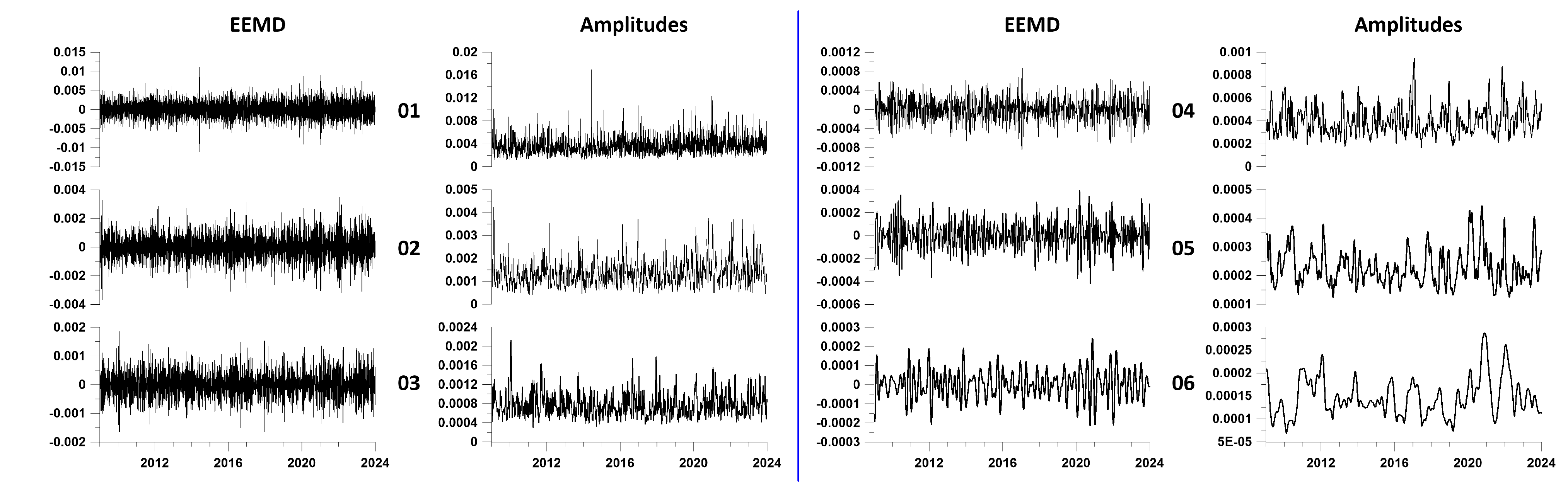
For each of the resulting 15 time series, EEMD waveforms of principal components were calculated. EEMD waveforms are obtained by averaging 1000 decompositions of the original signals, to which are added independent Gaussian white noises with a standard deviation of 0.1 from the standard deviation of the weighted average from each cluster. Figure 3 shows EEMD waveform plots for the first 6 expansion levels for three of the 15 clusters.
6. Hilbert Transform
The Hilbert transform of the signal is determined by the formula [53]:
where is the convolution of two functions. If and are the Fourier transforms of convolutional functions , then, as is known, the Fourier transform of convolution is equal to the product of the Fourier transforms of convolutional functions. Fourier transform from equals:
Thus, if there is a Fourier transform of , then
If you present , then
In practice, it is more convenient to calculate the Hilbert transform using the concepts of an analytical signal:
where are the amplitudes of the signal envelope, and is the instantaneous phase. The derivative is called instantaneous frequency. Fourier transform of the analytical signal or:
after which the Hilbert transform is equal to the imaginary part of the result of the inverse Fourier transform of
For each of the resulting 15 time series, EEMD waveforms of principal components were calculated. EEMD waveforms are obtained by averaging 1000 decompositions of the original signals, to which are added independent Gaussian white noises with a standard deviation of 0.1 from the standard deviation of the weighted average from each cluster. Figure 3 shows EEMD waveform plots for the first 6 expansion levels for three of the 15 clusters.
For a discrete-time signal , this transformation can be calculated using the discrete Fourier transform:
after which the 2nd part of the Fourier coefficients (corresponding to negative frequencies) should be reset to zero: while the 1st part should be doubled: . The Hilbert transform is then calculated as the imaginary part of the inverse discrete Fourier transform:
Thus, after determining the instantaneous amplitudes and frequencies of the EEMD, the Hilbert-Huang decomposition can be represented as follows:
Figure 4.
Plots of mean EEMD waveforms and mean instantaneous amplitudes averaged over all 15 station clusters for the first 6 decomposition levels. The left side of the figure, separated by a vertical blue line, shows pairs of graphs (waveforms - their amplitudes) for levels 1-3, and the right side shows graphs for levels 4-6. The decomposition level numbers are indicated between the waveform and amplitude graphs.
7. Influence Matrix
The next stage of the analysis is to study the connection between two sequences of random events. To solve this problem, a parametric intensity model is used. In [54,55,56] this method was used to test the hypotheses that local extrema of the average values of certain properties of seismic noise and magnetic field precede the instants of strong earthquakes.
Let represent the moments in time of 2 streams of events.
In our case it is:
1) a sequence of moments in time corresponding to the largest local maxima of the amplitudes of the envelopes at certain levels of the EEMD Huang decomposition
2) a sequence of times of seismic events with a magnitude not less than a given value.
Let's present their intensities in the form:
where are parameters, is the influence function of flow events with number :
According to formula (25), the weight of an event with number becomes non-zero for times and decays with a characteristic time . The parameter determines the degree of influence of the stream on the stream . The parameter determines the degree to which the flow influences itself (self-excitation), and the parameter reflects the purely random (Poisson) intensity component. Let us fix the parameter and consider the problem of determining the parameters .
The log-likelihood function for a non-stationary Poisson process is equal over the time interval [57]:
It is necessary to find the maximum of functions (26) with respect to the parameters . It is easy to obtain the following expression:
Since the parameters are non-negative, then each term on the left side of this formula is equal to zero at the maximum point of function (26) - either due to the necessary conditions for the extremum (if the parameters are positive), or, if the maximum is reached at the boundary, then the parameters themselves are equal to zero. Therefore, at the maximum point of the likelihood function the equality holds:
Let's substitute the expression from (28) into (27) and divide by . Then we get another form of formula (28):
where
- average value of the influence function. Substituting from (29) into (26), we obtain the following maximum problem:
where , under restrictions:
Function (31) is convex with a negative definite Hessian and, therefore, problem (31-32) has a unique solution. Having solved problem (31-32) numerically for a given , you can enter the elements of the influence matrix according to the formulas:
The value is part of the average intensity of the process with number , which is purely stochastic, part is caused by the influence of self-excitation and is due to external influence . From formula (29) the normalization condition follows:
As a result, the influence matrix can be determined:
The first column of matrix (35) is composed of Poisson fractions of average intensities. The diagonal elements of the right submatrix of size 2×2 consist of self-exciting elements of medium intensity, while the off-diagonal elements correspond to mutual excitation. The sums of the component rows of the influence matrix (34) are equal to 1. The influence matrices are estimated in a certain sliding time window of length with an offset and with a given value of the attenuation parameter .
8. Estimation of Connections between the Times of Local Amplitude Maxima and Seismic Events
The further plan of the article is to use the apparatus of influence matrices to assess the relationship between the times of maximum average amplitudes of the envelopes and the times of sufficiently strong earthquakes. A magnitude threshold of 5.5 was chosen. Such seismic events occurred in the vicinity of the Japanese islands during the period of time 2009-2023 it turned out to be 673 events - see Figure 5(a). However, the mega-earthquake of March 11, 2011 with a magnitude of 9 gave rise to a surge in aftershock activity, as a result of which, if we consider the time interval 2012-2023, when the intensity of aftershocks had already sharply decreased, the number of earthquakes with a magnitude of at least 5.5 will decrease by almost 2 times and become equal 349 – see Figure 5(b).
The working hypothesis is that for certain levels of EEMD decomposition, the times of the largest local maxima of the average amplitudes of the envelopes precedes the times of earthquakes. For a correct comparison of 2 streams of events, it is necessary that their average intensity be approximately equal. This means that the number of the largest local maxima of the amplitudes of the envelopes during the time period under study should be equal to the number of earthquakes. From these considerations, it becomes clear that for a correct analysis of the connections between the time instants of local maximum amplitudes of envelopes and seismic events, the time interval of aftershock activity must be excluded. Therefore, further analysis is carried out for the time period 2012-2023 lasting 12 years.
Figure 6 shows the distribution of epicenters of earthquakes with a magnitude of at least 5.5.
It should be taken into account that as the number of the decomposition level increases, both the waveforms of the levels themselves and the amplitudes of their envelopes become increasingly low-frequency. As a result, it is possible to select the 349 largest local maxima of average amplitudes in the interval 2012-2023 only for a certain number of lower expansion levels. For the time interval 2012-2023, only the first 2 levels are suitable for selecting 349 local maxima of amplitudes, since the number of local extrema already at the 3rd level is 242, that is, less than 349. From the first 2 levels, it was decided to choose the 2nd, as lower frequency, and for which the results of mutual influence assessments are more expressive.
In Figure 7, the red dots represent the selected 349 largest local maxima of the average amplitude of the envelopes at the 2nd level of decomposition.
Let us call the “direct” influence of the moments of time of earthquakes on the occurrence of local maxima of the average amplitudes of the envelopes, and the “reverse” - correspondingly, the advance of the moments of time of local maxima of amplitudes relative to the times of earthquakes. Figure 8 shows graphs of changes in the components of the matrix of “direct” and “reverse” influence for level 2 when assessed in a sliding window of 2 years.
of the model (23, 24) of 0.1 year. The graphs (a1, b1, c1) refer to the components of the influence matrix (34), which refers to the intensity fractions of the sequence of the largest local amplitude maxima, while the graphs (a2, b2, c2) refer to the intensity fractions of the sequence of seismic events. Other explanations in the text.
Of these graphs, the pair (a1, a2) is of greatest importance: a1 represents the change in the components of the direct influence of seismic events on the positions of local amplitude maxima, while a2 represents the inverse influence of the times of local amplitude maxima on seismic events. From a comparison of these two graphs, it is clear that the reverse influence significantly exceeds the direct one, that is, there is a delay effect of seismic events relative to the maximum amplitudes, in other words, there is a predictive effect. Graphs (b1, b2) represent changes in the self-exciting component of average intensities, while graphs (c1, c2) represent changes in the purely random (Poisson) component. Finally, the pair of plots (d1, d2) represents the change in the number of jointly analyzed time points in each time window. Let us recall once again that the sum of the components (a1, b1, c1) and (a2, b2, c2) is equal to 1 for any position of the time window.
Figure 8 presents the results of estimates of the mutual influence of two sequences of events only for a time window of 2 years. In order to increase the representativeness of this result, we will carry out similar estimates for a sufficiently large set of time lengths varying within specified limits. In this case, for each value of the length of the time window, we will identify local maxima of the components of the influence matrix, which are responsible for the mutual influence of sequences of events when the time windows are shifted. Let us describe a method for constructing a set of maximum components of mutual influence matrices in the form of numbered points.
- The minimum and maximum lengths of time windows and - the number of lengths of time windows in this interval are selected. Thus, the lengths of the time windows took on the values , , . In our calculations, we took equal to 1 year, and - 3 years, .
- Each time window of length was shifted from left to right along the time axis with some offset . Let us denote by , the sequence of moments in time of the positions of the right windows with length . The number of time windows in length is determined by their time offset . We used a time window offset of 0.01 year.
- For each position of a time window of length , the elements of the influence matrix (35) are estimated for a given relaxation time of the model (26-27), corresponding to the mutual influence of the two processes being analyzed. We took a value equal to 0.1 year. For definiteness, we will consider one influence, for example, of the first process on the second. As a result of such estimates, we obtain their values in the form , where is the corresponding element of the influence matrix for a position with a time window number of length .
- In the sequence , we select elements corresponding to local maxima of values , that is, from the condition . Let's present each element as a vertical segment of length located at a time point . The combination of such vertical graphic elements for all , visualizes the “strength” of the mutual influence of processes on each other.
So, the full set of free parameters of the method: , , , , . The result of such estimates is presented in Figure 9.
The results presented in Figure 9 confirm the conclusions made earlier based on the graphs in Figure 8: the “reverse” influence of the time instants of local maximums of envelope amplitudes at the 2nd level on the time instants of earthquakes is significantly greater (Figure 9(b)) than the “direct” influence of earthquakes on the occurrence of local maxima in the amplitudes of the envelopes (Figure 9(a)).
9. Conclusion
Traditional methods of analyzing data on crustal movements obtained using space geodesy are focused on identifying systematic low-frequency components that can be interpreted as manifestations of slow tectonic movements. The high-frequency component of these time series, which can be called the “tremor” of the earth's surface, is most often interpreted as a manifestation of noise arising from atmospheric and ionospheric fluctuations. Our point is that, despite the presence of this process noise, it is in the high-frequency component of GPS data that there is hidden prognostic information. In this article, the joint use of cluster analysis, principal component analysis, Hilbert-Huang decomposition and evaluation of parametric models of the mutual influence of sequences of events allowed us to obtain a result confirming the presence of predictive information in high-frequency tremor of the earth's surface.
Author Contributions
A.L. – idea, programming, paper preparation; E.R. – programming, data preparation.
Funding
This research received no external funding.
Institutional Review Board Statement
Not applicable.
Data Availability Statement
The open access data from the source: http://geodesy.unr.edu/gps_timeseries/tenv3/IGS14/ (accessed on 15 January 2024) were used.
Acknowledgments
The work was carried out within the framework of the state assignment of the Institute of Physics of the Earth of the Russian Academy of Sciences (topic FMWU-2022-0018).
Conflicts of Interest
The authors declare that the research was conducted in the absence of any commercial or financial relationships that could be construed as a potential conflict of interest.
References
- Lyubushin, A. Identification of Areas of Anomalous Tremor of the Earth's Surface on the Japanese Islands According to GPS Data. Applied Sciences, 2022, 12:7297. [CrossRef]
- Lyubushin, A. Singular Points of the Tremor of the Earth's Surface. Applied Sciences, 2023, 13:10060. [CrossRef]
- Lyubushin, A. Entropy of GPS-measured Earth tremor. In: Revolutionizing Earth Observation - New Technologies and Insights. Editor: Rifaat M. Abdalla. IntechOpen. 2024. [CrossRef]
- Lyubushin, A. Global coherence of GPS-measured high-frequency surface tremor motions. GPS Solutions, 2018, 22:116. [CrossRef]
- Lyubushin, A. Field of coherence of GPS-measured earth tremors. GPS Solutions, 2019, 23:120. [CrossRef]
- Filatov, D.M.; Lyubushin, A.A. Fractal analysis of GPS time series for early detection of disastrous seismic events. Phys A, 2017, 469(1):718-730. [CrossRef]
- Filatov, D.M.; Lyubushin, A.A. Precursory Analysis of GPS Time Series for Seismic Hazard Assessment. Pure and Applied Geophysics, 2019, 177(1):509-530. [CrossRef]
- Huang, N.E.; Shen, Z.; Long, S.R.; Wu, V.C.; Shih, H.H.; Zheng, Q.; Yen, N.C.; Tung, C.C.; Liv, H.H. The empirical mode decomposition and the Hilbert spectrum for nonlinear and non-stationary time series analysis. Proc. Roy. Soc. London Ser. A. 1998, 454:903-995. [CrossRef]
- Huang, N. E., and Z. Wu. A review on Hilbert-Huang transform: Method and its applications to geophysical studies. Rev. Geophys, 2008, 46:RG2006. [CrossRef]
- Pan, Y.; Shen, W.-B.; Ding, H.; Hwang, C.; Li, J.; Zhang, T. The Quasi-Biennial Vertical Oscillations at Global GPS Stations: Identification by Ensemble Empirical Mode Decomposition. Sensors, 2015, 15:26096-26114. [CrossRef]
- Li, W. Extraction of periodic signals in Global Navigation Satellite System (GNSS) vertical coordinate time series using the adaptive ensemble empirical modal decomposition method. Nonlin. Processes Geophys, 2024, 31:99–113. [CrossRef]
- Huang, Y.; Schmitt, F.G.; Lu, Zh.; Liu, Y. Analysis of daily river flow fluctuations using empirical mode decomposition and arbitrary order Hilbert spectral analysis. Journal of Hydrology, 2009, 373:103–111. [CrossRef]
- Huang, N.E.; Wu, M.; Qu, W.; Long, S.R. and Shen S.S.P. Applications of Hilbert–Huang transform to non-stationary financial time series analysis. Appl. Stochastic Models Bus. Ind, 2003, 19:245–268. [CrossRef]
- Li, H. , Kwong S., Yang L., Huang D., and Xiao D. Hilbert-Huang Transform for Analysis of Heart Rate Variability in Cardiac Health. IEEE/ACM Trans Comput Biol Bioinform, 2011, 8(6):1557-1567. [CrossRef]
- Wei, H.-Ch. , Xiao M.-X., Chen H.-Y., Li Y.-Q., Wu H.-T. and Sun Ch.-K. Instantaneous frequency from Hilbert-Huang transformation of digital volume pulse as indicator of diabetes and arterial stiffness in upper-middle-aged subjects. Scientific Reports, 2018, 8:15771. [CrossRef]
- Beavan, J. Noise properties of continuous GPS data from concrete pillar geodetic monuments in New Zealand and comparison with data from U.S. deep drilled braced monuments. J Geophys Res, 2005, 110:B08. [CrossRef]
- Langbein, J. Noise in GPS displacement measurements from Southern California and Southern Nevada. J. Geophys. Res. 2008, 113, B05405. [Google Scholar] [CrossRef]
- Blewitt, G.; Hammond, W.C.; Kreemer, C. Harnessing the GPS data explosion for interdisciplinary science. Eos 2018, 99, 485. [Google Scholar] [CrossRef]
- Bos, M. S., R. M. S. Fernandes, S. D. P. Williams, and L. Bastos, Fast error analysis of continuous GPS observations, J. Geod. 2008, 82, 157–166. [Google Scholar] [CrossRef]
- Liu, B.; Xing, X.; Tan, J.; Xia, Q. Modeling Seasonal Variations in Vertical GPS Coordinate Time Series Using Independent Component Analysis and Varying Coefficient Regression. Sensors 2020, 20, 5627. [Google Scholar] [CrossRef]
- Liu, B.; Dai, W.; Liu, N. Extracting seasonal deformations of the Nepal Himalaya region from vertical GPS position time series using Independent Component Analysis. Adv. Space Res., 2017, 60:2910-2917. [CrossRef]
- Tesmer, V.; Steigenberger, P.; van Dam, T.; Mayer-Gurr, T. Vertical deformations from homogeneously processed GRACE and global GPS long-term series. J. Geod. 2011, 85, 291–310. [Google Scholar] [CrossRef]
- Yan, J.; Dong, D.; Burgmann, R.; Materna, K.; Tan, W.; Peng, Y.; Chen, J. Separation of Sources of Seasonal Uplift in China Using Independent Component Analysis of GNSS Time Series. J. Geophys. Res. Solid Earth 2019, 124, 11951–11971. [Google Scholar] [CrossRef]
- Santamarнa-Gуmez, A.; Memin, A. Geodetic secular velocity errors due to interannual surface loading deformation. Geophys. J. Int. 2015, 202, 763–767. [Google Scholar] [CrossRef]
- Fu, Y.; Argus, D.F.; Freymueller, J.T.; Heflin, M.B. Horizontal motion in elastic response to seasonal loading of rain water in the Amazon Basin and monsoon water in Southeast Asia observed by GPS and inferred from GRACE. Geophys. Res. Lett. 2013; 40:6048-6053. [CrossRef]
- Chanard, K.; Avouac, J.P.; Ramillien, G.; Genrich, J. Modeling deformation induced by seasonal variations of continental water in the Himalaya region: Sensitivity to Earth elastic structure. J. Geophys. Res. Solid Earth 2014, 119, 5097–5113. [Google Scholar] [CrossRef]
- He, X.; Montillet, J.P.; Fernandes, R.; Bos, M.; Yu, K.; Hua, X.; Jiang, W. Review of current GPS methodologies for producing accurate time series and their error sources. J. Geodyn. 2017, 106, 12–29. [Google Scholar] [CrossRef]
- Ray, J.; Altamimi, Z.; Collilieux, X.; van Dam, T. Anomalous harmonics in the spectra of GPS position estimates. GPS Solutions 2008, 12, 55–64. [Google Scholar] [CrossRef]
- Roncagliolo, P.A. , Garcнa J.G., Mercader P.I., Fuhrmann D.R., Muravchik C.H. Maximum-likelihood attitude estimation using GPS signals. Digital Signal Processing 2007, 17, 1089–1100. [Google Scholar] [CrossRef]
- Wang, F.; Li, H.; Lu, M. GNSS Spoofing Detection and Mitigation Based on Maximum Likelihood Estimation. Sensors 2017, 17, 1532. [Google Scholar] [CrossRef]
- Parkinson, B.W. Global Positioning System: Theory and Applications; AIAA: Reston, VA, USA, 1996. 781 p.
- Jing Xu, Jingsha He, Yuqiang Zhang, Fei Xu, and Fangbo Cai. A Distance-Based Maximum Likelihood Estimation Method for Sensor Localization in Wireless Sensor Networks. International Journal of Distributed Sensor Networks 2016, Article ID 2080536. [CrossRef]
- Langbein J, Johnson H. Correlated errors in geodetic time series, Implications for time-dependent deformation. J Geophys Res. 1997; 102(B1):591–603. [CrossRef]
- Williams, S.D.P.; Bock, Y.; Fang, P.; Jamason, P.; Nikolaidis, R.M.; Prawirodirdjo, L.; Miller, M.; Johnson, D.J. Error analysis of continuous GPS time series, J. Geophys. Res. 2004, 109, B03412. [Google Scholar] [CrossRef]
- Wang, W.; Zhao, B.; Wang, Q.; Yang, S. Noise analysis of continuous GPS coordinate time series for CMONOC. Adv. Space Res. 2012, 49, 943–956. [Google Scholar] [CrossRef]
- Agnew, D. The time domain behavior of power law noises, Geophys. Res. Lett. 1992; 19:333-336. [CrossRef]
- Amiri-Simkooei, A. R., C. C. J. M. Tiberius, and P. J. G. Teunissen Assessment of noise in GPS coordinate time series: Methodology and results, J. Geophys. Res. B: 2007; 112, 2007. [Google Scholar] [CrossRef]
- Caporali, A. Average strain rate in the Italian crust inferred from a permanent GPS network—I. Statistical analysis of the time-series of permanent GPS stations. Geophys. J. Int. 2003, 155, 241–253. [Google Scholar] [CrossRef]
- Zhang, J.; Bock, Y.; Johnson, H.; Fang, P.; Williams, S.; Genrich, J.; Wdowinski, S.; Behr, J. Southern California permanent GPS geodetic array: Error analysis of daily position estimates and site velocities. J. Geophys. Res. 1997, 102, 18035–18055. [Google Scholar] [CrossRef]
- Li, J.; Miyashita, K.; Kato, T.; Miyazaki, S. GPS time series modeling by autoregressive moving average method, Application to the crustal deformation in central Japan. Earth Planets Space 2000, 52, 155–162. [Google Scholar] [CrossRef]
- Kermarrec, G. , Schon, S. On modelling GPS phase correlations: a parametric model. Acta Geod Geophys. 2018; 53:139-156. [CrossRef]
- Teferle, F.N.; Williams, S.D.P.; Kierulf, H.P.; Bingley, R.M.; Plag, H.P. A continuous GPS coordinate time series analysis strategy for high-accuracy vertical land movements. Phys. Chem. Earth Parts A/B/C 2008, 33, 205–216. [Google Scholar] [CrossRef]
- Chen, Q.; van Dam, T.; Sneeuw, N.; Collilieux, X.; Weigelt, M.; Rebischung, P. Singular spectrum analysis for modeling seasonal signals from GPS time series. J. Geodyn. 2013, 72, 25–35. [Google Scholar] [CrossRef]
- Bock Y, Melgar D, Crowell, B. W. Real-Time Strong-Motion Broadband Displacements from Collocated GPS and Accelerometers. Bull. Seismol. Soc. Am. 2011, 101, 2904–2925. [Google Scholar] [CrossRef]
- Goudarzi, M.A.; Cocard, M.; Santerre, R.; Woldai, T. GPS interactive time series analysis software. GPS Solut. 2013, 17, 595–603. [Google Scholar] [CrossRef]
- Hackl, M.; Malservisi, R.; Hugentobler, U.; Jiang, Y. Velocity covariance in the presence of anisotropic time correlated noise and transient events in GPS time series. J. Geodyn. 2013, 72, 36–45. [Google Scholar] [CrossRef]
- Khelif, S.; Kahlouche, S.; Belbachir, M.F. Analysis of position time series of GPS-DORIS co-located stations. Int. J. Appl. Earth Observ. Geoinf. 2013, 20, 67–76. [Google Scholar] [CrossRef]
- Blewitt, G.; Hammond, W.C.; Kreemer, C. Harnessing the GPS data explosion for interdisciplinary science. Eos 2018, 99, 485. [Google Scholar] [CrossRef]
- Duda, R.O.; Hart, P.E.; Stork, D.G. Pattern Classification; Wiley: Hoboken, NJ, USA, 2000. [Google Scholar]
- Vogel, M.A. and Wong A.K.C., PFS clustering method, IEEE Trans. Pattern Anal. Mach. Intell, 1979, 1(3):237-45. [CrossRef]
- Jolliffe, I.T. Principal Component Analysis; Springer: Berlin/Heidelberg, Germany, 1986. [Google Scholar]
- Huber P.J. Robust statistics. N.Y.; Chichester, Brisbane; Toronto: Wiley, 1981.
- Bendat J.S., Piersol A.G. Random Data. Analysis and Measurement Procedures. Fourth Edition. Wiley & Sons. New Jersey, 2010.
- Lyubushin A Investigation of the Global Seismic Noise Properties in Connection to Strong Earthquakes. Front. Earth Sci. 2022, 10:905663. [CrossRef]
- Lyubushin, A. Seismic Hazard Indicators in Japan based on Seismic Noise Properties. Journal of Earth and Environmental Sciences Research, 2023, 5(8):1-8. [CrossRef]
- Lyubushin, A. , Rodionov E. Wavelet-based correlations of the global magnetic field in connection to strongest earthquakes. Advances in Space Research, 2024. [CrossRef]
- Cox D.R., Lewis P.A.W. The statistical analysis of series of events. London, Methuen, 1966.
Figure 1.
1(a) shows the positions of 1047 GPS stations and their division into 15 clusters. The numbered circles indicate the centers of gravity of the clusters, and the blue lines indicate the boundaries between Voronoi cells. The blue star shows the position of the center of mass of all cluster centers. Figure 1(b) shows a plot of the pseudo-F-statistic that allowed us to select 15 as the number of clusters.
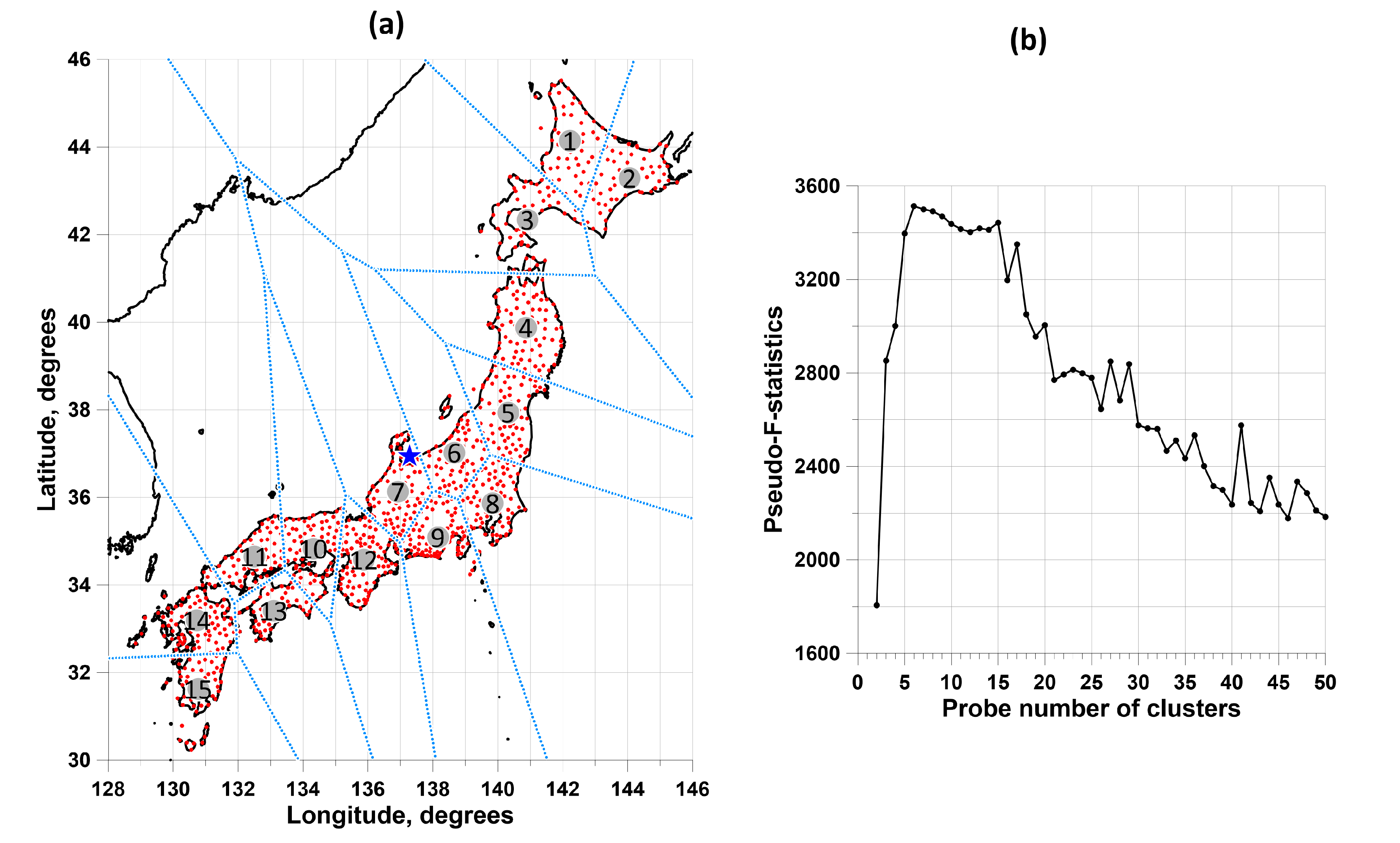
Figure 2.
Graphs of weighted average vertical displacements of the earth's surface in each of the selected 15 clusters in a sliding time window of 365 days. The Y axes represent displacement increments in mm.
Figure 2.
Graphs of weighted average vertical displacements of the earth's surface in each of the selected 15 clusters in a sliding time window of 365 days. The Y axes represent displacement increments in mm.
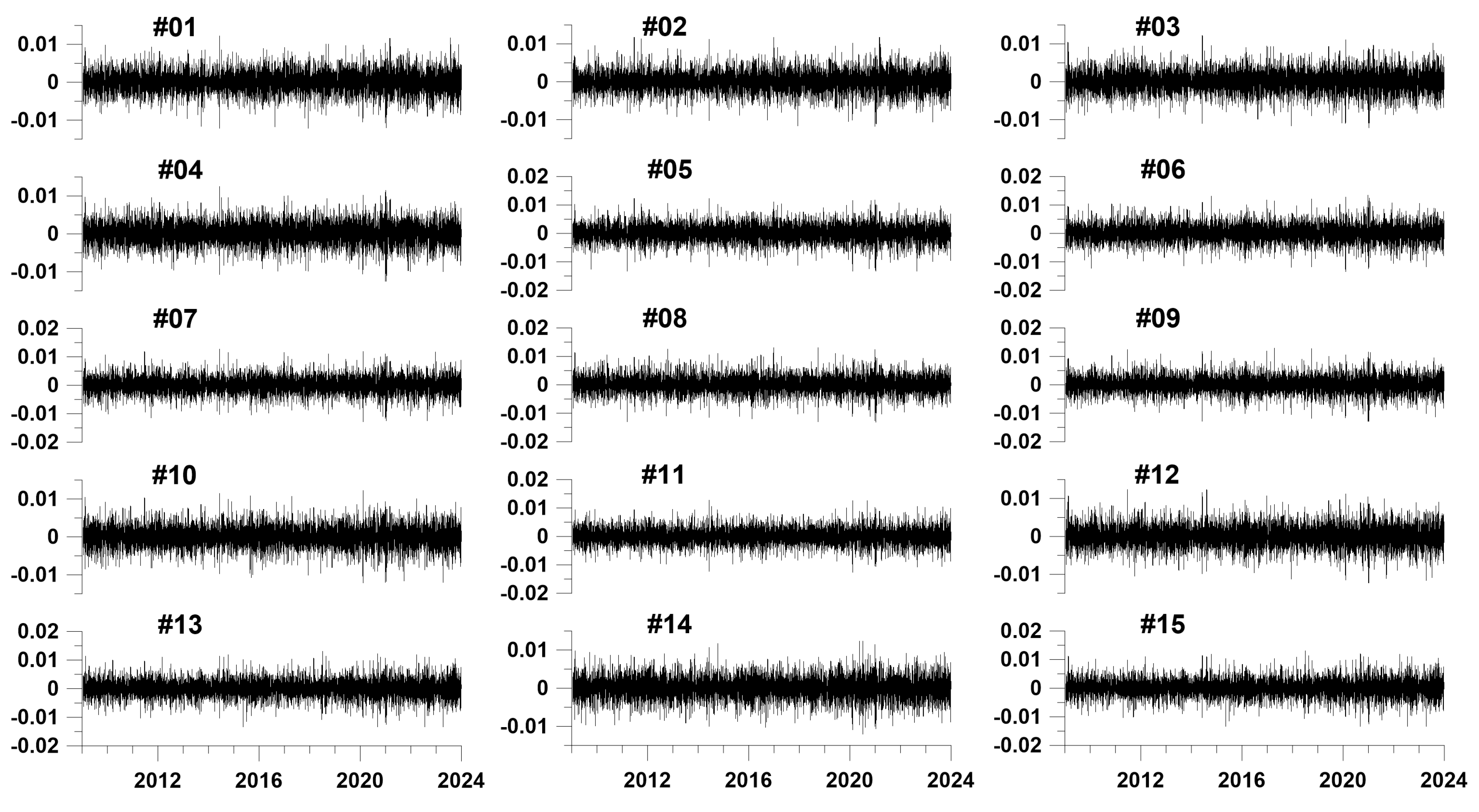
Figure 3.
EEMD waveform plots for the first 6 decomposition levels for 3 clusters (numbers 1, 9 and 15). Decomposition level numbers are indicated on the left.
Figure 3.
EEMD waveform plots for the first 6 decomposition levels for 3 clusters (numbers 1, 9 and 15). Decomposition level numbers are indicated on the left.
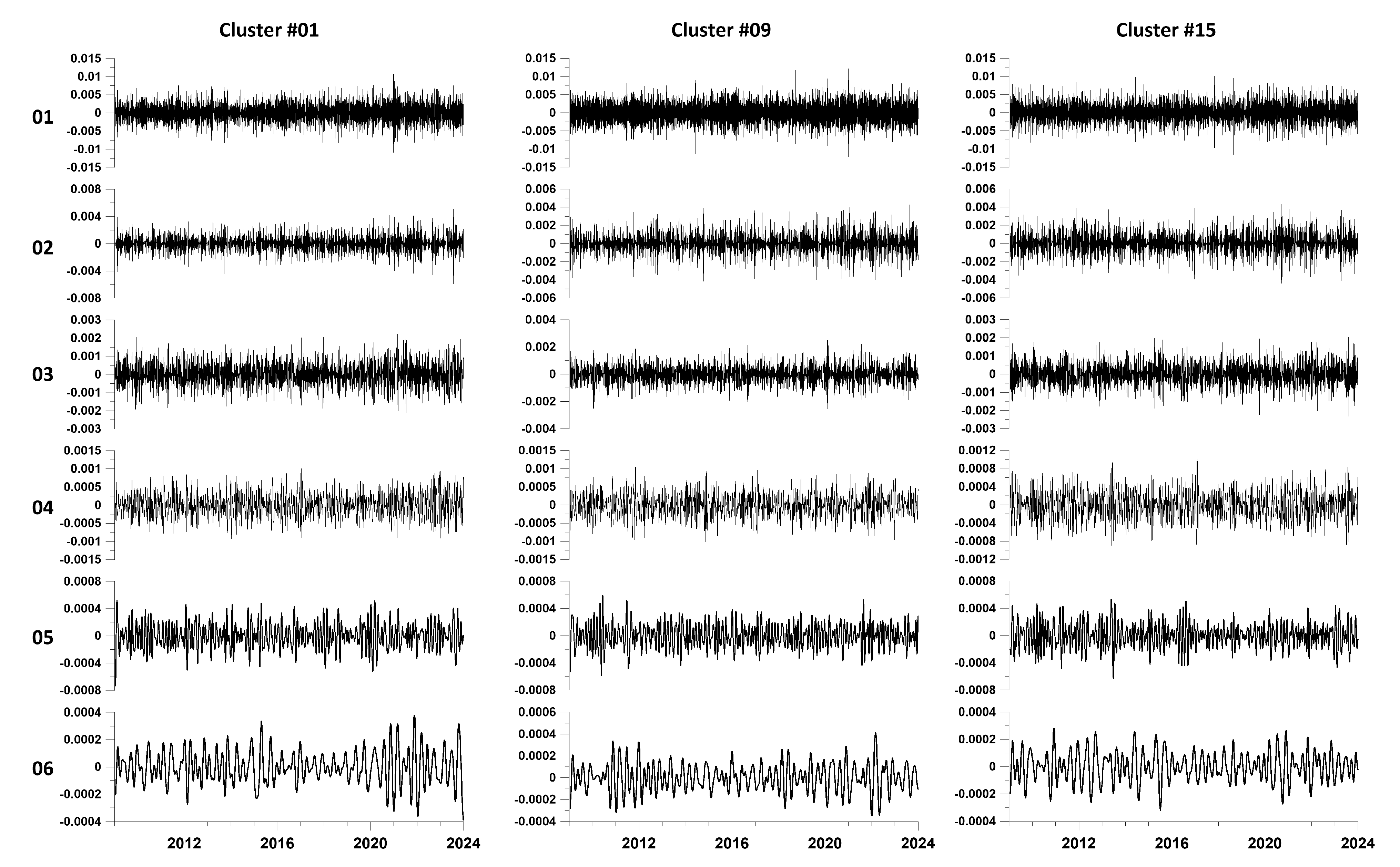
Figure 5.
Time sequence of earthquakes with a magnitude of at least 5.5 in the vicinity of the Japanese Islands: (a) - in the time period 2009-2023; (b) – in the period of time 2012-2023.
Figure 5.
Time sequence of earthquakes with a magnitude of at least 5.5 in the vicinity of the Japanese Islands: (a) - in the time period 2009-2023; (b) – in the period of time 2012-2023.
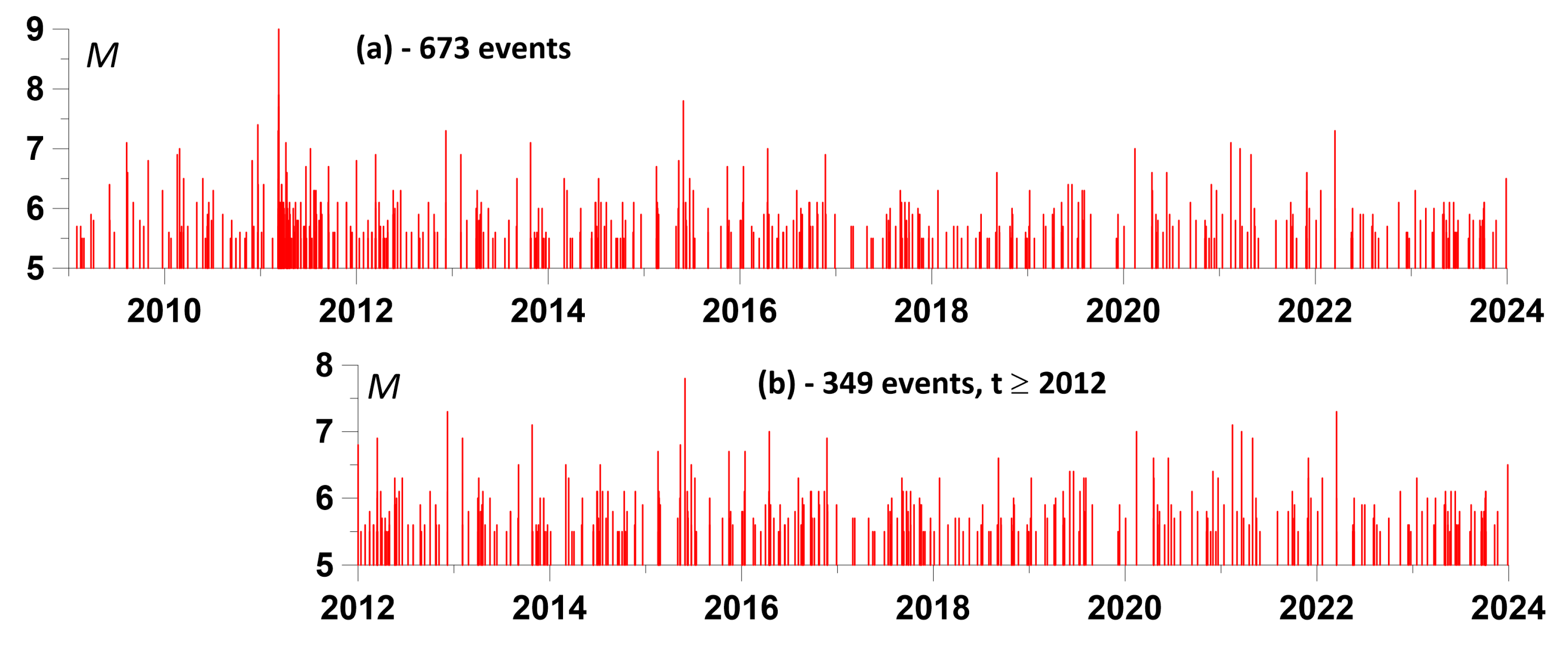
Figure 6.
Distribution of epicenters of 349 earthquakes with a magnitude of at least 5.5 in the vicinity of the Japanese Islands in the time period 2012-2023. The red asterisk marks the center of gravity of the centers of 15 clusters of GPS stations (Figure 1(a)), which is chosen as the center of a circle with a radius of 1500 km.
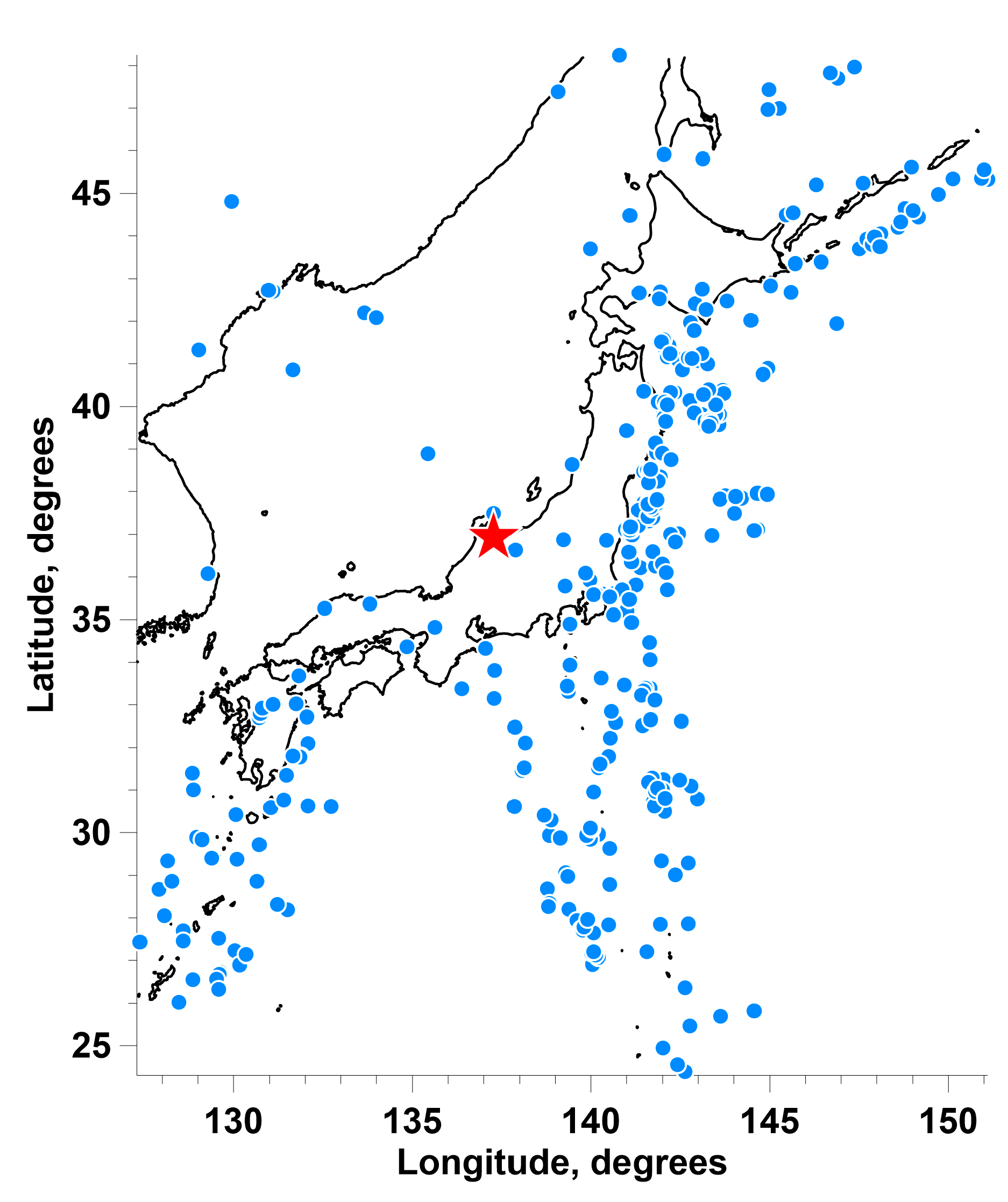
Figure 7.
Average instantaneous amplitudes of the 2nd level of EEMD decomposition and the 349 largest local maxima (red dots).
Figure 7.
Average instantaneous amplitudes of the 2nd level of EEMD decomposition and the 349 largest local maxima (red dots).
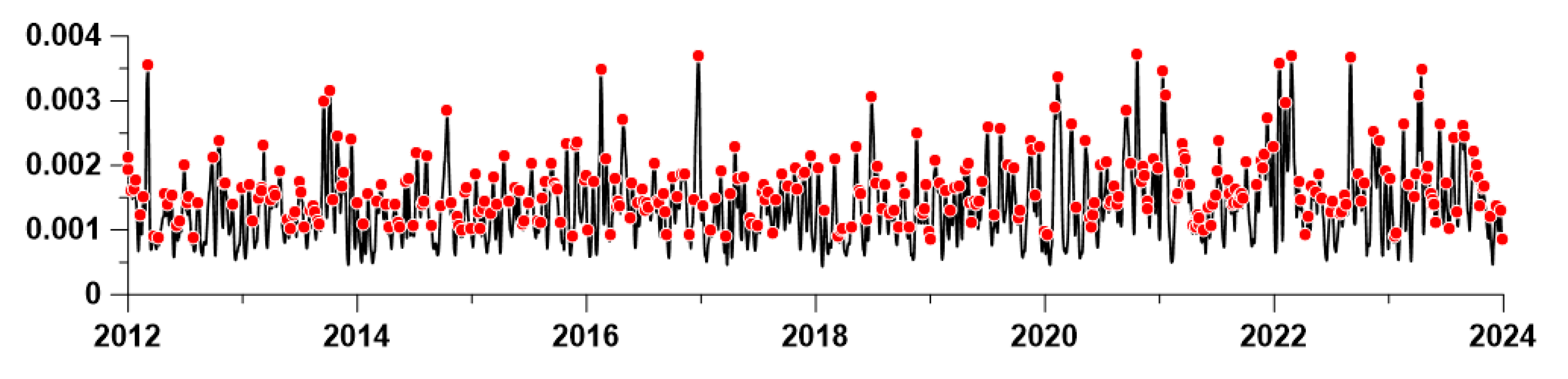
Figure 8.
Graphs of changes in the components of the influence matrix between sequences of seismic events with a magnitude of at least 5.5 and the sequence of moments in time 349 of the largest local maxima of the average amplitudes at the 2nd level of EEMD decomposition. The estimates were made in a sliding time window of length 2 years with a shift of 0.01 year for a relaxation time
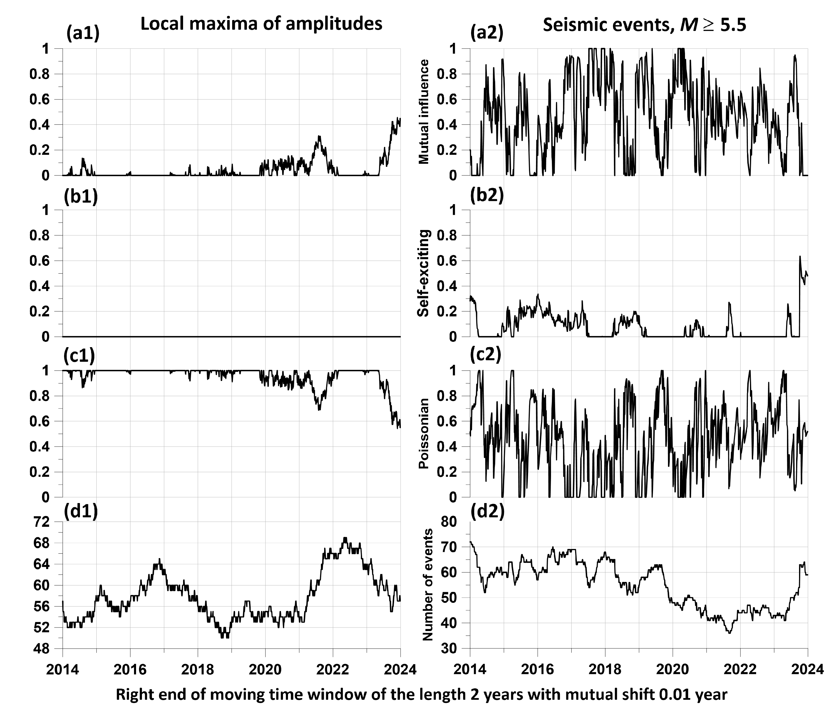
Figure 9.
Maximum values of the elements of the influence matrices in a sequence of 100 time windows of length from 1 to 3 years, taken with an offset of 0.01 year: (a) - for the “direct” influence of the time points of seismic events on the positions of the largest local maximums of average amplitudes on the 2nd EEMD level of decomposition; (b) – for the “reverse” influence of the positions of amplitude maxima on earthquakes. The relaxation time of the model is 0.1 year.
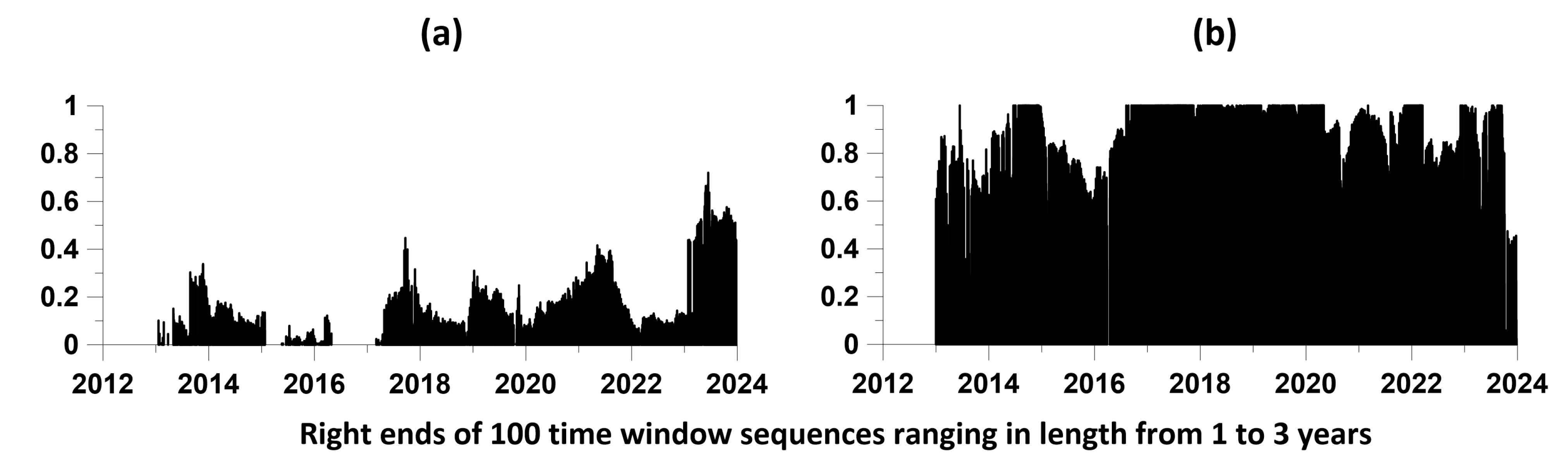

Table 1.
Number of Nsta stations in each Clust# cluster.
| Clust# | 1 | 2 | 3 | 4 | 5 | 6 | 7 | 8 | 9 | 10 | 11 | 12 | 13 | 14 | 15 |
| Nsta | 57 | 56 | 54 | 83 | 69 | 61 | 78 | 77 | 91 | 76 | 57 | 95 | 48 | 88 | 57 |
Disclaimer/Publisher’s Note: The statements, opinions and data contained in all publications are solely those of the individual author(s) and contributor(s) and not of MDPI and/or the editor(s). MDPI and/or the editor(s) disclaim responsibility for any injury to people or property resulting from any ideas, methods, instructions or products referred to in the content. |
© 2024 by the authors. Licensee MDPI, Basel, Switzerland. This article is an open access article distributed under the terms and conditions of the Creative Commons Attribution (CC BY) license (http://creativecommons.org/licenses/by/4.0/).
Copyright: This open access article is published under a Creative Commons CC BY 4.0 license, which permit the free download, distribution, and reuse, provided that the author and preprint are cited in any reuse.


