
Submitted:
22 December 2024
Posted:
23 December 2024
You are already at the latest version
Abstract
The hypothesis of occurrence of meteorological anomalies before earthquakes is investigated. Long-term time series of observations for air temperature, atmospheric pressure and precipitation at the meteorological station on Kamchatka are considered. Time series are subjected to Huang decomposition into sequences of levels of empirical oscillation modes (intrinsic mode functions - IMF) forming a set of orthogonal components with increasing average frequency. For each IMF level, instantaneous amplitudes of the envelopes are calculated using the Hilbert transform. Comparison with the earthquake sequence is made using a parametric model of the intensity of two interacting point processes, which allows one to quantitatively estimate the "measure of the lead" of the time instants of the compared sequences. For each IMF level the number of time moments of the largest local maxima of instantaneous amplitudes which is equal to the number of earthquakes was selected. As a result of the analysis, it turned out that for the 6th IMF level (periods of 8-16 days), the "lead measure" of the instantaneous amplitude maxima of meteorological parameters in comparison with earthquake time moments significantly exceeds the inverse lead, which confirms the existence of prognostic changes in meteorological parameters in the problem of the "atmosphere-lithosphere" interaction.
Keywords:
atmosphere-lithosphere interaction
; meteorological time series
; seismic process
; Hilbert-Huang decomposition
; instantaneous amplitudes
; interacting point processes
; Kamchatka
1. Introduction
In the study of the interaction of processes at the lithosphere-atmosphere boundary, one of the intriguing questions is the study of the relationship between the variability of meteorological conditions in the near-surface conditions of the Earth with the final stages of preparation of strong earthquakes. Consideration of this question is especially relevant in relation to the problem of forecasting earthquakes based on possible meteorological precursors.
A number of publications have demonstrated the effect of increasing temperature and decreasing humidity of the surface air of the atmosphere before strong and moderate earthquakes [1,2,3,4,5,6]. An explanation of this phenomenon is given within the framework of the model of complex relationships in the lithosphere-atmosphere and ionosphere-magnetosphere (LAIMC) system [7]. According to LAIMC, at the final, relatively short-term stage of earthquake preparation, thermal anomalies in the atmosphere at low altitudes may form due to the release of latent heat of evaporation during condensation of water vapor on ions due to the ionization of air molecules by alpha particles emitted by nuclei of radioactive gases, mainly radon, entering the atmosphere from the upper horizons of the earth's crust.
Verification of the LAIMC model requires the presence of indisputable data on the occurrence of anomalous radon flows from the Earth's surface on the eve of strong earthquakes or on establishing a connection between data from long-term meteorological observations in seismically active regions, in particular data on surface air temperature, with earthquakes that have occurred.
Observations of the volumetric activity of radon in near-surface conditions are usually of an experimental nature. In addition to reports of the phenomenon of an increase in the volumetric activity of soil gaseous radon, there are also data on a decrease in its activity before earthquakes [8]. Therefore, the question of anomalous discharges of gaseous radon from the lithosphere into the atmosphere before strong earthquakes remains open to this day.
A promising direction in studying processes at the lithosphere-atmosphere boundary during earthquake preparation is the use of long-term meteorological observations in seismically active regions. Such observations are carried out on the basis of metrologically supported methods for issuing weather forecasts, assessing the state of the natural environment, etc. In the work of the authors [9], using observation data from meteorological stations in the seismically active region of the Kamchatka Peninsula, the relationship between increased and decreased values of air temperature and atmospheric pressure, as well as their contrasting changes, at the final stages of preparation of local strong earthquakes accompanied by noticeable tremors was analyzed. In this work, an empirical method of comparing their average daily values with the behavior of annual average seasonal functions was used to identify anomalous changes in meteorological parameters. In addition, formalized statistical methods were used to identify anomalies in the behavior of three statistics characterizing the variability of time series of air temperature and atmospheric pressure in a sliding time window of 112 days with a step of 1 day. Using empirical and statistical methods for processing time series of meteorological parameters, anomalous effects were identified at time intervals of 7, 30 and 112 days and their seismic forecasting significance in relation to the strong earthquakes that occurred. The detection of the random nature of the manifestation of various types of meteorological anomalies before the earthquakes under consideration, as well as the absence of a systematic manifestation of the effect of an abnormal increase in air temperature before earthquakes, cast doubt on the realism of generating thermal near-surface anomalies of atmospheric air at the short-term stage of preparation of strong seismic events in the Kamchatka region.
It should be noted that in the mentioned work [9], the assignment of time intervals of 7, 30 and 112 days, during which the manifestation of a relationship between surface meteorological anomalies and earthquake preparation processes was assumed, was made on the assumption of a relatively short-term manifestation of thermal effects before strong earthquakes. While the study of various types of earthquake precursors in the Kamchatka Peninsula area shows that the characteristic durations of their manifestation before earthquakes range from days-months to the first years [10,11,12]. This demonstrates the need to develop methods for analyzing the relationship between meteorological parameters and the seismic process, allowing such a relationship to be analyzed in a wide range of periods of its manifestation, including the months and years preceding strong Kamchatka earthquakes.
This paper continues the study of the relationship between anomalies in time series of meteorological parameters and the seismic process in Kamchatka, the first results of which were presented in [9]. In this paper, the Huang method was used to decompose long-term meteorological time series, which allows constructing a sequence of orthogonal oscillations for each series, which are called "internal oscillation modes" in the method. The Hilbert transform of the sequence of these oscillation modes makes it possible to obtain sequences of instantaneous amplitudes and frequencies. The paper studies the relationship between the time points of maxima of instantaneous amplitudes of meteorological parameter series and the time moments of strong earthquakes using a parametric model of interacting point processes. The result of the study is the discovery of the effect of leading the time points of maxima of instantaneous amplitudes of air temperature of the time moments of earthquakes at the low-frequency level of the Huang decomposition.
2. Initial Data
The work used meteorological observation data and data on earthquakes that occurred in the Kamchatka Peninsula region for the period from November 4, 1996 to September 30, 2024 (10193 days). A total of 27 years 11 months (27.9 years).
Meteorological Data
The data of observations of atmospheric pressure, air temperature and precipitation at the Pionerskaya meteorological station of the Kamchatka Territorial Administration for Hydrometeorology and Environmental Monitoring (53.08° N, 158.55° E) from the database of the POLYGON Information System of the Kamchatka Branch of the Geophysical Service of the Russian Academy of Sciences were used [13] (accessed October 1, 2024).
At the Pionerskaya meteorological station, a meteorological mercury thermometer with a division value of 0.2°C is used to measure the air temperature. It is located in a protective wooden booth at a height of 2 m above the earth's surface. Atmospheric pressure was measured with a mercury barometer. Precipitation was measured with a precipitation vessel installed on a horizontal surface at a height of 2 m and protected from gusts of wind. The amount of precipitation is the height of the water layer in mm formed by rain, drizzle, melted snow and hail.
The sampling step of meteorological observations and the corresponding discretization of time series of meteorological parameters is 3 hours (Figure 1).
Earthquake Data
To characterize the seismic process in the Kamchatka Peninsula area during the period from November 4, 1996 to September 30, 2024, a sample of 418 earthquakes with local magnitudes that occurred in the depth range from 0 to 635 km in the responsibility area of the Kamchatka Branch of the Geophysical Survey of the Russian Academy of Sciences (KB GS RAS) was used. The earthquake sampling was carried out from the Kamchatka and Commander Islands Earthquake Catalogue: (http://www.gsras.ru/new/infres/, [ID 85], accessed October 1, 2024) using the Unified Information System of Seismological Data KB GS RAS [14] and the Interactive Map of the Distribution of Earthquake Epicenters from the Kamchatka and Commander Islands Earthquake Catalogue (see https://sdis.emsd.ru/map/).
Figure 2 shows the epicenters of all 418 earthquakes, the boundaries of the KB GS RAS area of responsibility, and the location of the Pionerskaya weather station.
In the catalog of Kamchatka and the Commander Islands compiled by KB GS RAS, the representative energy class of earthquakes (decimal logarithm of seismic energy output) for the entire responsibility zone is and corresponds to the local magnitude . To obtain the studied sample of earthquakes, earthquakes with for the considered time period were selected from the specified catalog. The magnitudes in the sample of earthquakes were recalculated from the values of the energy classes using the formula [15]. Thus, setting the minimum magnitude obviously ensured the representativeness of the resulting sample of 418 earthquakes for the entire territory of the KB GS RAS responsibility zone.
The 418 earthquakes under consideration have magnitudes . The table presents data on the strongest earthquakes that occurred according to KB GS RAS data and data on their moment magnitudes from the USGS/NEIS catalog.

Table 1.
Data on the strongest earthquakes that occurred in the KB GS RAS area of responsibility according to: https://sdis.emsd.ru/info/earthquakes/catalogue.php , https://earthquake.usgs.gov/earthquakes/search/.
Table 1.
Data on the strongest earthquakes that occurred in the KB GS RAS area of responsibility according to: https://sdis.emsd.ru/info/earthquakes/catalogue.php , https://earthquake.usgs.gov/earthquakes/search/.
| Date yyyymmdd |
Time hh:mm:ss |
Latitude, φ, N ° |
Longitude, λ, E ° |
Depth, km |
ML |
R, km |
MW NEIC |
L, km |
R/L |
| 20030616 | 22:08:02 | 55.30 | 160.34 | 190 | 6.6 | 331 | 6.9 | 50 | 6.7 |
| 20031205 | 21:26:14 | 55.78 | 165.43 | 29 | 6.7 | 533 | 6.7 | 41 | 13.1 |
| 20040610 | 15:19:55 | 55.68 | 160.25 | 208 | 6.7 | 370 | 6.9 | 50 | 7.4 |
| 20060420 | 23:24:28 | 60.98 | 167.37 | 1 | 7.1 | 1019 | 7.6 | 100 | 10.2 |
| 20081124 | 9:02:52 | 53.77 | 154.69 | 564 | 6.8 | 623 | 7.3 | 74 | 8.4 |
| 20121116 | 18:12:39 | 49.06 | 155.87 | 78 | 6.7 | 486 | 6.5 | 33 | 14.5 |
| 20130228 | 1:05:48 | 50.67 | 157.77 | 61 | 6.8 | 271 | 6.9 | 50 | 5.4 |
| 20130301 | 13:20:49 | 50.64 | 157.90 | 62 | 6.8 | 272 | 6.5 | 33 | 8.1 |
| 20130524 | 5:44:47 | 54.75 | 153.79 | 630 | 7.8 | 726 | 8.3 | 199 | 3.6 |
| 20131001 | 3:38:19 | 52.88 | 153.34 | 608 | 6.8 | 700 | 6.7 | 41 | 17.1 |
| 20160130 | 3:25:08 | 53.85 | 159.04 | 178 | 7.1 | 200 | 7.2 | 67 | 3.0 |
| 20170329 | 4:09:22 | 56.97 | 163.22 | 43 | 6.8 | 521 | 6.6 | 37 | 14.1 |
| 20170602 | 22:24:47 | 53.99 | 170.55 | 32 | 6.6 | 795 | 6.8 | 45 | 17.6 |
| 20170717 | 23:34:08 | 54.35 | 168.90 | 7 | 7.3 | 692 | 7.7 | 110 | 6.3 |
| 20181013 | 11:10:20 | 52.53 | 153.87 | 499 | 7.0 | 592 | 6.7 | 41 | 14.5 |
| 20181220 | 17:01:54 | 54.91 | 164.71 | 54 | 7.3 | 448 | 7.3 | 74 | 6.1 |
| 20200325 | 2:49:20 | 49.11 | 158.08 | 48 | 7.7 | 438 | 7.5 | 90 | 4.9 |
| 20230403 | 3:06:56 | 52.58 | 158.78 | 105 | 6.6 | 120 | 6.5 | 33 | 3.6 |
| 20240817 | 19:10:25 | 52.79 | 160.38 | 43 | 7.0 | 126 | 7.0 | 55 | 2.3 |
Note: R is the hypocentral distance to the Pionerskaya weather station, is the size of the earthquake source, calculated using the formula [17].
3. Research Method
3.1. Empirical Mode Decomposition
Let be some analyzed time series with discrete time index.
Empirical mode decomposition (EMD) [18,19] represents the decomposition of the signal into empirical oscillation modes:
where is the j-th empirical mode, is the remainder, is the number of empirical modes.
The algorithm for decomposing into a sequence of empirical modes is iterative for each level . We denote by the iteration index: , where is the maximum number of iterations for level . The iterations are described by the formula
Here , where and are the upper and lower envelopes for the signal , which are constructed using spline interpolation (usually a 3rd order spline) over all local maxima and minima of the signal .
Iterations (2) are initialized with a zero step for the first level () of the expansion . Then the upper and lower envelopes and are found, the average line is calculated and is found using formula (2). For the upper and lower envelopes and are determined and the average line , is found, and so on, up to the last iteration index , after which the first empirical mode is considered to be found.
The condition for stopping the iterations is usually chosen in the form of the inequality:
where is some small number, such as 0.01. Once the mode is found, an iterative process is started to determine the empirical mode of the next level. This process is initialized by the formula for the initial iteration index :
According to formula (4), the high-frequency part is subtracted from the original signal and the resulting, lower-frequency signal is considered as a new signal for subsequent decomposition. The construction of empirical oscillation modes continues until the number of local extrema becomes too small to be used to construct envelopes.
As the empirical mode level number increases, the signals become increasingly low-frequency and tend to an unchangeable form. The sequence is constructed in such a way that its sum gives an approximation to the original signal , which can be represented as (1) [18,19].
Empirical modes of oscillations, known as Intrinsic Mode Functions (IMF), are orthogonal to each other, thus constituting a certain empirical basis for the decomposition of the original signal. In what follows, the decomposition levels will be called IMF levels.
In practical implementation of the method, technical difficulties arise due to edge effects, since the behavior of envelopes beyond the first and last points of local extrema is ambiguous. There are several approaches to overcome this difficulty, in particular, a mirror continuation of the analyzed sample back and forth over a sufficiently long period of time. It was used in this work.
3.2. Ensemble Empirical Mode Decomposition
One of the key drawbacks of the EMD method is the problem of mode mixing, which occurs when one empirical mode includes signals of different scales or when signals of the same scale are distributed among different empirical modes. For example, if the signal exhibits "intermittency", i.e. short-term sections of higher-frequency behavior appear against the background of a smooth signal, then the EMD decomposition results in mixing of behavior modes with different frequencies, since the relatively rare points of local extrema of smooth behavior alternate with significantly more frequent points of local extrema of the high-frequency component.
To overcome this effect, Huang and Wu [19] proposed the ensemble empirical mode decomposition (EEMD) method. It is a regularization of the EMD method in which finite-amplitude white noise is added to the original data. This allows the true empirical modes to be determined as the average over an ensemble of trials, each of which is the sum of the signal and white noise.
The EEMD algorithm includes the following steps:
1. Add a white noise realization to the original data.
2. Decompose the white noise-added data into empirical modes.
3. Repeat steps 1 and 2 a sufficiently large number of times with independent white noise realizations.
4. Obtain an ensemble mean for the corresponding empirical modes.
In this way, numerous “artificial” observations are simulated in the real time series:
where is the i-th independent realization of white noise.
The true component in the behavior of time series, according to the EEMD definition, for a sequence of all levels of empirical modes is calculated as their average value of the expansions of artificially noisy modes (5).
It is important to note that the use of EEMD largely eliminates the above-mentioned mode mixing problem [Huang and Wu, 2008]. Adding independent white noise to the sample has a regularizing effect, since it simplifies the construction of envelopes (after adding a small white noise, there are immediately many local extrema). The operation of averaging over a sufficiently large number of independent realizations of white noise allows one to get rid of the influence of the noise component and to isolate the true internal modes of oscillations of time series of meteorological parameters.
For each of the time series (Figure 1), EEMD waveforms were calculated by averaging 2000 decompositions of the original signals, to which independent Gaussian white noise with a standard deviation equal to 0.1 of the standard deviation of each decomposed signal was added.
3.3. Hilbert Transform
The Hilbert transform [20] of a signal is determined by the formula:
where – convolution of two functions. If и – Fourier transforms of convoluted functions,, then, as is known, the Fourier transform of a convolution is equal to the product of the Fourier transforms of the functions being convolved. The Fourier transform of equals:
Thus, if is a Fourier transform of , then
If present , then
Let be some analyzed time series with discrete time index.
In practice, it is more convenient to calculate the Hilbert transform using the concepts of an analytical signal:
where are the amplitudes of the signal envelope, and is the instantaneous phase. The derivative is called the instantaneous frequency. The Fourier transform of the analytical signal can be written as:
after which the Hilbert transform is equal to the imaginary part of the result of the inverse Fourier transform of :
For a discrete-time signal , this transform can be calculated using the discrete Fourier transform:
after which the 2nd part of the Fourier coefficients (corresponding to negative frequencies) should be set to zero : while the 1st part should be doubled . After this, the Hilbert transform is calculated as the imaginary part of the inverse discrete Fourier transform:
Thus, after determining the instantaneous amplitudes and frequencies of the EEMD, the Hilbert-Huang expansion can be represented as follows:
In the work [21], the Hilbert-Huang expansion was used to search for the predictive properties of the tremor of the earth's surface measured by space geodesy on the Japanese islands.
The further plan of action was to compare the times of the largest local maxima of the correlations between the amplitudes of the envelopes at different levels with the times of sufficiently strong earthquakes. In this case, the number of the largest local maxima of the correlations of the amplitudes of the envelopes is chosen to be equal to the number of seismic events under consideration.
Below, in Figure 3, Figure 4 and Figure 5, the EEMD waveform graphs are presented for levels 1 to 12 of all time series of meteorological parameters, the amplitude graphs of their envelopes and instantaneous frequencies calculated using the Hilbert transform.
The Hilbert-Huang decomposition resembles the wavelet decomposition in its form (functionally): as in the wavelet decomposition, with an increase in the IMF level number, the corresponding component becomes increasingly low-frequency. However, there is a significant difference, which lies in the dependence of both the amplitude and the frequency on time, which is expressed by formula (15). In the orthogonal wavelet decomposition, the frequency band corresponding to the detail level with the number is fixed and corresponds to the frequency interval , where , , where is the discretization step in time [22]. In the Hilbert-Huang decomposition, there is no such one-to-one correspondence. Therefore, to estimate the characteristic frequency of each IMF level, a value equal to the time average of all instantaneous frequency values was used. Figure 6 shows the average values of instantaneous frequencies of meteorological parameters depending on the IMF level number.
3.4. Influence Matrix
The next stage of the analysis is the study of the relationship between two sequences of random events, which in this study represent the sequence of the largest local maxima of the envelopes of the initial series of meteorological parameters determined by the algorithm described above, and the sequence of 418 earthquakes with .
To solve this problem, a parametric model of the intensity of two point processes is used.
Previously, in [23,24], this method was used to test the hypotheses that local extremes of the mean values of certain seismic noise and magnetic field statistics precede the times of strong earthquakes. In [21], this model was used to estimate the seismic forecasting properties of the positions of local maxima of instantaneous amplitudes of the envelopes of ground tremor on the Japanese islands, measured by GPS.
Let's consider the computational algorithm. Let represent the moments of time of 2 streams of events. In our case, these are:
1) a sequence of time moments corresponding to the largest local maxima of the envelope amplitudes at some IMF levels of the EEMD decomposition;
2) the sequence of times of seismic events with a magnitude not less than a given value (in our case, with a magnitude of ML≥5.5).
Let us represent the intensities of these two streams of events as follows:
where are the parameters, is the influence function of events of the flow with number :
According to formula (16), the weight of the event with number becomes non-zero for times and decays with characteristic time . The parameter determines the degree of influence of the flow on the flow . The parameter determines the degree of influence of the flow on itself (self-excitation), and the parameter reflects a purely random (Poisson) component of intensity. Let us fix the parameter and consider the problem of determining the parameters .
The log-likelihood function for a non-stationary Poisson process is equal to over the time interval [25]:
It is necessary to find the maximum of functions (18) with respect to parameters . It is easy to obtain the following expression:
Since the parameters must be non-negative, each term on the left side of formula (19) is equal to zero at the point of maximum of function (18) – either due to the necessary conditions of the extremum (if the parameters are positive), or, if the maximum is reached at the boundary, then the parameters themselves are equal to zero. Consequently, at the point of maximum of the likelihood function, the equality is satisfied:
Let's substitute the expression from (20) into (19) and divide by . Then we get another form of formula (20):
where
- the average value of the influence function. Substituting from (21) into (18), we obtain the following maximum problem:
where , under restrictions:
Function (23) is convex with negative definite Hessian and, therefore, problem (23-24) has a unique solution. Having solved problem (23-24) numerically for a given , we can introduce the elements of the influence matrix according to the formulas:
The quantity is a part of the average intensity of the process with a number , which is purely stochastic, the part is caused by the influence of self-excitation and is determined by the external influence . From formula (21) follows the normalization condition:
As a result, we can determine the influence matrix:
The first column of matrix (27) is composed of Poisson shares of average intensities. The diagonal elements of the right submatrix of size consist of self-excited elements of average intensity, while the off-diagonal elements correspond to mutual excitation. The sums of the component rows of the influence matrix (27) are equal to 1.
3.5. Relationship Between Local Maxima of the Instantaneous Amplitudes of Meteorological Parameters and Seismic Events
The further plan is to use the influence matrix apparatus to assess the relationship between the times of maximum amplitudes of the envelopes of meteorological time series and the times of strong earthquakes.
The threshold of local earthquake magnitudes for the Kamchatka Peninsula region in the KB GS RAS control zone was defined as . There were 418 such seismic events during the studied period (average recurrence of 15 events/year or 1.25 events/month).
The working hypothesis was investigated, which consisted in the fact that for certain levels of decomposition, the moments of time of the largest local maxima of the amplitudes of the envelope meteorological parameters "on average" precede the moments of time of earthquakes. In confirming this hypothesis, we assume that the maxima of meteorological parameters precede the occurrence of strong earthquakes, i.e. there is an effect of an advanced connection between meteorological parameters and strong earthquakes.
For a correct comparison of two event flows, their average intensities must be approximately equal. This means that the number of the largest local maxima of the amplitudes of the envelopes of meteorological parameter series must be equal to the number of earthquakes, i.e. 418. It should also be taken into account that with an increase in the number of the decomposition level, both the waveforms of the levels themselves and the amplitudes of their envelopes become increasingly low-frequency. As a result, it is possible to select 418 largest local maxima of the amplitudes of the envelopes only for a certain number of lower decomposition levels.
As a result of sorting through the IMF levels for all three series of the EEMD decomposition (Figure 3, Figure 4 and Figure 5), the 6th IMF level was chosen as the optimal one, for which the “direct” influence of the moments of time of the largest local maxima of the amplitudes of the envelopes on the moments of time of seismic events with a magnitude of at least 5.5 significantly exceeded the “reverse” influence.
This means that in the range of low instantaneous frequencies of the 6th level of decomposition, the amplitudes of the envelopes of meteorological time series precede the moments of time of sufficiently strong earthquakes and one can assume the presence of a prognostic effect.
Another possibility for extracting the amplitudes of the envelopes of narrow-band components of time series is to use wavelet decomposition with subsequent calculation of the amplitudes of the envelopes from each level of detail using the Hilbert transform. However, this method turned out to be less effective for studying the leading influence of meteorological parameters on seismic events than the Hilbert-Huang decomposition, with the exception of the air temperature time series. The behavior of the air temperature time series is quite smooth (Figure 1b), as a result of which the optimal Daubechies wavelet with 10 vanishing moments was determined for this time series from the condition of minimum entropy of the distribution of squares of wavelet coefficients [22]. The prognostic effect of such an analysis of the air temperature time series turned out to be most effective for the 6th detail level using wavelet decompositions. With a sampling time step of 3 hours, this level corresponds to a range of periods of 8-16 days, that is, it is in the low-frequency range of 0.53-0.27 month-1.
Figure 7(a) shows a sequence of earthquakes with magnitudes . Then, Figure 7(b, c, d) show the graphs of the envelope amplitudes at the 6th IMF level of the EEMD decomposition of the time series of atmospheric pressure, air temperature and precipitation. In addition, Figure 7(e) shows the graph of the envelope amplitude of the wavelet decomposition of the air temperature time series at the 6th level of detail using the Daubechies wavelet with 10 vanishing moments.
When analyzing variations of the components of influence matrices in sliding time windows corresponding to the mutual influence of the analyzed time sequences, the main attention is paid to their local maxima with their subsequent averaging. Below is described a method for processing these local maxima and averaging them for a set of time window lengths changing within specified limits.
1. The minimum and maximum lengths of time windows are selected and - the number of lengths of time windows in this interval. Thus, the lengths of time windows took the values , , . In our calculations, we took equal to 4 years, and - 7 years, .
2. Each time window of length shifted from left to right along the time axis with some offset . Let us denote by , the sequence of time moments of the positions of the right windows of length . The number of time windows of length is determined by their time offset . We used a time window offset of 0.05 years.
3. For each position of the time window of length , the elements of the influence matrix (27) are estimated for a given relaxation time of the model (16-17), corresponding to the mutual influence of the two analyzed processes. We took a value equal to 0.5 years. For definiteness, we will consider some one influence, for example, of the first process on the second. As a result of such estimates, we obtain their values in the form , where is the corresponding element of the influence matrix for the position with the number of the time window of length .
4. In the sequence , we select elements corresponding to local maxima of values , that is, from the condition .
5. We choose a "small" time interval of length and for a sequence of such time fragments we calculate the average value of local maxima for which their time marks belong to these fragments. Averaging is performed over all lengths of time windows. In our calculations we took the length equal to 0.1 years.
Thus, the complete set of free parameters of the influence matrix method is: , , , , , .
4. Average Values of the Components of the Influence Matrices
Figure 8 (a1, b1, c1) shows the graphs of the average values of the components of the influence matrices of the sequence of the largest local maxima of the envelopes of time series of atmospheric pressure, air temperature and precipitation at the 6th IMF level of their EEMD decomposition into a sequence of earthquakes with a magnitude of МL≥5.5 for 100 lengths of time windows from 4 to 7 years.
Figure 8(d1) shows the graph of the average value of the influence matrices of the largest local maxima of the amplitudes of the envelope of the wavelet decomposition of the air temperature time series for the 6th detail level on earthquakes. Finally, Figure 8 (e1) shows the “secondary” average value of all average components of the influence matrices in Figure 8 (a1, b1, c1, d1).
The graphs in the right column of Figure 8 (a2, b2, c2, d2, e2) show all the average values of the components of the influence matrices, corresponding to the “reverse” advance of the earthquake sequence on the positions of the largest local amplitudes of all time series of meteorological parameters.
The red lines in Figure 8 represent the average values for all time window positions in the range of windows lengths from 4 to 7 years.
The graphs in Figure 8 show a pronounced leading (predictive) effect of the behavior of the amplitude maxima of the envelopes of meteorological time series in relation to seismic events. In this case, the maximum average value of the averaged components of the influence matrices of 0.426 was obtained for the air temperature time series (Figure 8 d1). The inverse influence of seismic events on the behavior of meteorological parameter series is significantly lower, and for the air temperature series it becomes negligibly small (Figure 8 b2, d2).
In all diagrams in the left column of the graphs in Figure 8, systematic bursts of the influence of local maxima of the amplitudes of the envelopes of time series of meteorological parameters on seismic events occur in 2011-2012, which preceded the seismicity activation in the Kamchatka Peninsula area in 2013, which included four strong seismic events, including the Sea of Okhotsk earthquake of 24.05.2013 with (Table 1), which is the strongest seismic event during the period of detailed seismological observations in Kamchatka since 1962. In individual diagrams in Figure 8 (a1, d1, e1), this maximum can be traced from 2007, i.e., during the period of up to 6 years preceding the sharp increase in the activity of strong earthquakes in Kamchatka.
The next surge in the leading influence of local maxima of meteorological parameters on the seismic process in 2019-2020 (Figure 8) preceded the earthquake of March 25, 2020 with a magnitude of in the southern part of the considered area and the activation of seismicity immediately near the Pionerskaya meteorological station, including the earthquakes of April 3, 2023, and August 17, 2024, (Table 1). While the activation of seismicity in the northern part of the considered area in 2017-2018 was not accompanied by the leading manifestation of local maxima of meteorological parameters. This allows us to assume a certain connection between the manifestations of the discovered seismic prognostic effect of the advanced increase in the amplitudes of the envelope meteorological parameters with the relative proximity of earthquake foci and, possibly, with their seismotectonic localization.
The graph in Figure 8(e1) describes a strong averaging of local maxima of the component of the influence matrices corresponding to the “direct” advance of the set of meteorological parameters of local maxima of the moments of time of earthquakes with magnitudes of at least 5.5. In this case, averaging was performed for all three analyzed meteorological parameters, assuming that their changes occur in an interconnected manner and are controlled mainly by the advection of air masses due to their global movements in the Kamchatka Peninsula area.
At the same time, from the analysis of the left column of the graphs in Figure 8, it is evident that the local maxima of the envelopes of the precipitation series (graphs 8(c1) demonstrate the least prognostic effect, compared to the atmospheric pressure and air temperature series. Therefore, the components of the influence matrices were averaged only for the atmospheric pressure and air temperature series. As a result, a graph was obtained (Figure 9), similar to that shown in Figure 8(e1), but with the exception of the precipitation time series.
5. Discussion
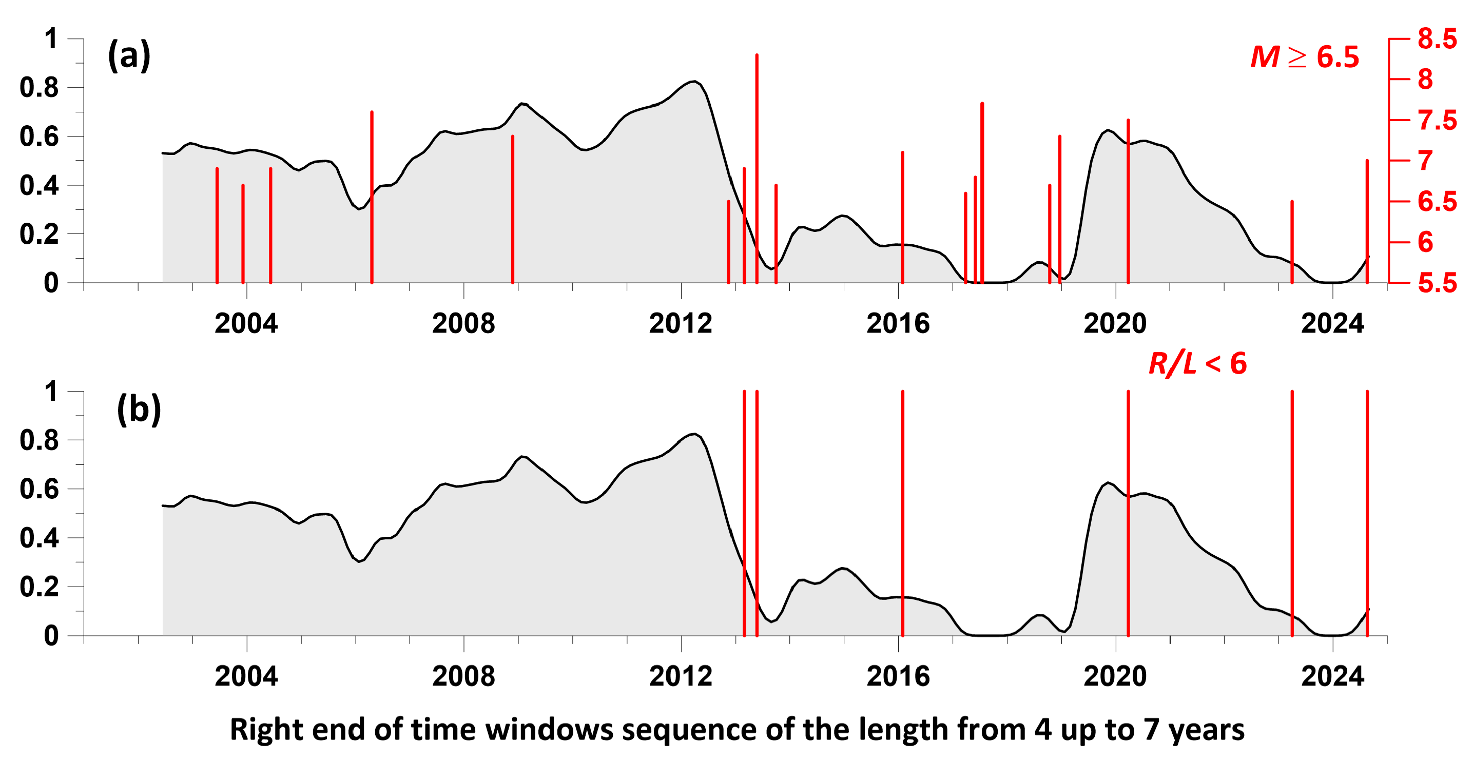
The graph in Figure 9 allows us to compare the behavior of the components of the averaged influence matrices for two time series of meteorological parameters both with the moments of the strongest earthquakes (Figure 9(a))) and taking into account the proximity of the location of the foci of strong earthquakes in relation to the Pionerskaya meteorological station (Figure 9(b)).
To characterize the proximity of individual strong earthquakes in relation to the location of the weather station, we used the ratio, where is the epicentral distance to the Pionerskaya weather station, km; is the characteristic size of the earthquake source (in km) depending on its magnitude. The calculation of was carried out using the formula [17]. Thus, the value (Table 1) shows the distance of the earthquake from the weather station in the number of earthquake source sizes and can be considered as an indicator of the intensity of the earthquake preparation process in the area of the weather station.
The lower panel of Figure 9 shows only those earthquakes for which the value of , i.e. when these earthquakes occurred, the meteorological stations were located within the middle (intermediate) zone of their sources. There were only 6 such earthquakes. These were the strongest events, which were accompanied in the area of the meteorological station by tremors with an intensity of 4 to 5-6 points on the MSK-64 scale, and for them the ratio .
Let us consider the manifestations of the maxima of the averaged graph of the components of the influence matrices of the largest local maxima of the amplitudes of the envelopes of the atmospheric pressure and air temperature series with the time distribution of the strongest earthquakes, as well as the closest of the strong earthquakes in relation to the weather station. It is evident that the manifestations of the local maxima of the graph precede the three strongest earthquakes with magnitudes , and with a characteristic lead time of such maxima of 1.5 – 2 years. The earthquakes of 2023 () and 2024 (), which occurred at a relatively short distance from the weather station ( and ), were not accompanied by preceding maxima in the changes of the components of the influence matrices. The same applies to the strong seismic events of 2017-2018, which occurred at distances of 450-800 km from the weather station within the junction of the Kuril-Kamchatka and Aleutian seismically active regions.
It should be concluded that the proposed method for identifying meteorological prognostic anomalies is mainly focused on the general seismic activity or, figuratively speaking, on the "seismic temperature" of the region. Therefore, identifying prognostic anomalies before specific strong earthquakes is not yet reliable and requires further research in this direction. As for the assessment of the average measure of the lead time of the largest local maxima of instantaneous amplitudes relative to the time of the flow of earthquakes with a magnitude of at least 5.5, shown in Figure 9, a strong non-stationarity of this measure, the presence of both a strong lead and almost zero, is of particular interest. This non-stationarity can be caused by the impact of atmospheric events in the Pacific Ocean, such as typhoons, and can also be the subject of further research in the problem of interaction of processes in the "atmosphere-lithosphere" system.
6. Conclusions
A method for analyzing the relationship between long-term meteorological observation data and the seismic process is proposed and implemented using the example of the Kamchatka seismically active region using the decomposition of meteorological time series by the Huang method and the construction of a sequence of orthogonal oscillations (intrinsic modes functions) for each series. Using the Hilbert transform, sequences of distribution of instantaneous amplitudes were obtained from the sequence of these oscillation modes, which were compared with the moments of strong earthquakes within the framework of a parametric model of interacting point processes.
The most important result of the study is the detection of the effect of advance of time points of maximum instantaneous amplitudes of air temperature, atmospheric pressure and precipitation of earthquake time moments at the low-frequency (6th) IMF level of Huang decomposition. This indicates the detection of the effect of advance connection between changes in meteorological parameters, primarily air temperature, and the occurrence of strong earthquakes for characteristic periods of variations of 8-16 days.
The manifestation of maxima of average values of the components of the influence matrices of the largest local maxima of the amplitudes of the envelopes of atmospheric pressure and air temperature series was detected with a lead time of 1.5-2 years before three strong earthquakes in the Kuril-Kamchatka seismic active zone with magnitudes of 8.3, 7.2 and 7.5, which occurred at relative distances from the meteorological station . To obtain more substantiated estimates of the seismic forecasting properties of the graphs of average values of the components of the influence matrices of the largest local maxima of the amplitudes of the envelopes of meteorological parameter series in relation to the strongest () earthquakes in the region, as well as the closest of such earthquakes in relation to the observation area, it is necessary to conduct additional studies.
Supplementary Materials
The following supporting information can be downloaded at the website of this paper posted on Preprints.org. The original meteorological data are contained in the database of the Kamchatka branch of the Geophysical Service of the Russian Academy of Sciences: http://www.gsras.ru/new/infres/ , POLYGON Information System (Database of Geophysical Observations), ID 21. To obtain data for scientific research purposes, please contact G. N. Kopylova, co-author of this work, by e-mail: gala@emsd.ru .
Author Contributions
AL – idea of the research, writing the text, data processing; GK – writing the text, ER – data processing, YS – data preparing. All authors have read and agreed to the published version of the manuscript.
Funding
This research received no external funding.
Institutional Review Board Statement
Not applicable
Informed Consent Statement
Not applicable
Data Availability Statement
The original meteorological data are contained in the database of the Kamchatka branch of the Geophysical Service of the Russian Academy of Sciences: http://www.gsras.ru/new/infres/ , POLYGON Information System (Database of Geophysical Observations), ID 21. To obtain data for scientific research purposes, please contact G. N. Kopylova, co-author of this work, by e-mail: gala@emsd.ru .
Acknowledgments
The work was carried out within the framework of the state assignments of the Institute of Physics of the Earth of the Russian Academy of Sciences and Kamchatka branch of the Geophysical Service of the Russian Academy of Sciences.
Conflicts of Interest
The authors declare that the research was conducted in the absence of any commercial or financial relationships that could be construed as a potential conflict of interest.
References
- Dunajecka, M.A. and Pulinets, S.A., Atmospheric and thermal anomalies observed around the time of strong earthquakes in Mexico, Atmosfera, 2005, 18, 4:235-247.
- Genzano, N., Filizzaola, C., Hattori, K., Pergola, N., and Tramutoli, V., Statistical correlation analysis between thermal infrared anomalies observed from MTSATs and large earthquakes occurred in Japan (2005-2015), J. Geophys. Res.: Solid Earth, 2021, 126(2), Article ID e2020-JB020108. [CrossRef]
- Hayakawa, M., Izutsu, J., Schekotov, A., Yang, S.-S., Solovieva, M., and Budilova, E., Lithosphere-atmosphere-ionosphere coupling effects based on multiparameter precursor observations for February-March 2021 earthquakes (M~7) in the offshore of Tohoku area of Japan, Geosciences, 2021, 11(11), Article ID 481. [CrossRef]
- Ouzounov, D., Pulinets, S., Kafatos, M.C., and Taylor, P., Thermal radiation anomalies associated with major earthquakes, in Pre-Earthquakes Processes: A Multidisciplinary Approach to Earthquake Prediction Studies, AGU Geophys. Monogr. Ser., 2018, 234: 259-274, New York: Wiley. [CrossRef]
- Editors: Ouzounov, D., Pulinets, S., Kafatos, M.C., and Taylor, P., Pre-Earthquakes Processes: A Multidisciplinary Approach to Earthquake Prediction Studies, AGU Geophys. Monogr. Ser., vol. 234, New York: Wiley, 2018. [CrossRef]
- Shitov A.V., Pulinets S.A., Budnikov P.A. Effect of Earthquake Preparation on Changes in Meteorological Characteristics (Based on the Example of the 2003 Chuya Earthquake), Geomagnetism and Aeronomy, 2023, 63, 4:395-408. [CrossRef]
- Pulinets, S.A., Ouzounov, D.P., Karelin, A.V., and Davidenko, D.V. Physical bases of the generation of short-term earthquake precursors: A complex model of ionization-induced geophysical processes in the lithosphere-atmosphere-ionosphere-magnetosphere system. Geomagn. Aeron., 2015, 55, 4:521-538. [CrossRef]
- Cicerone R.D., Ebel J.E., Beitton J.A. Systematic compilation of earthquake precursors, Tectonophysics, 2009, 476:371-396. [CrossRef]
- Kopylova G.N., Serafimova Yu.K., Lyubushin A.A. Meteorological Anomalies and Strong Earthquakes: A Case Study of the Petropavlovsk-Kamchatsky Region, Kamchatka Peninsula. Izvestiya, Physics of the Solid Earth, 2024, 60, 3:494-507. [CrossRef]
- Konovalova A.A., Saltykov V.A. Seismic Precursors of Large (M 6.0) Earthquakes in the Junction Zone between the Kuril-Kamchatka and Aleutian Island Arcs. Journal of Volcanology and Seismology, 2023, 17, 6:60-77. [CrossRef]
- Gavrilov V.A., Panteleev I.A., Deshcherevskii A.V., Lander A.V., Morozova Yu.V., Buss Yu.Yu., Vlasov Yu.A. Stress-Strain State Monitoring of the Geological Medium Based on The Multi-instrumental Measurements in Boreholes: Experience of Research at the Petropavlovsk-Kamchatskii Geodynamic Testing Site (Kamchatka, Russia). Pure Appl. Geophys. 2020, 177:397-419. [CrossRef]
- Kopylova G., Boldina S. Hydrogeological Earthquake Precursors: A Case Study from the Kamchatka Peninsula. Front. Earth Sci. 2020. 8:576017. [CrossRef]
- Kopylova G. N., V. Yu. Ivanov, V. A. Kasimova, The implementation of information system elements for interpreting integrated geophysical observations in Kamchatka. Russ. J. Earth Sci., 2009, 11, ES1006. [CrossRef]
- Chebrova A.Yu., Chemarev A.S., Matveenko E.A., Chebrov D.V. Seismological data information system in Kamchatka branch of GS RAS: organization principles, main elements and key functions. Geophysical Research, 2020, 21, 3:66-91. https://portal.ifz.ru/journals/gr/21-3/fulltext/05-GR-21-3.pdf (in Russian). [CrossRef]
- Chubarova O.S., Gusev A.A., Chebrov V.N. The ground motion excited by the Olyutorskii earthquake of April 20, 2006 and by its aftershocks based on digital recordings, Journal of Volcanology and Seismology, 2010, 4, 2:126-138. [CrossRef]
- Zelenin, E., Bachmanov, D., Garipova, S., Trifonov, V., and Kozhurin, A.: The Active Faults of Eurasia Database (AFEAD): the ontology and design behind the continental-scale dataset, Earth Syst. Sci. Data, 2022, 14, 10:4489-4503. [CrossRef]
- Zavyalov A.D., Zotov O.D. A new way to determine the characteristic size of the source zone. Journal of Volcanology and Seismology, 2021, 15, 1:19-25. [CrossRef]
- Huang, N.E.; Shen, Z.; Long, S.R.; Wu, V.C.; Shih, H.H.; Zheng, Q.; Yen, N.C.; Tung, C.C.; Liv, H.H. The empirical mode decomposition and the Hilbert spectrum for nonlinear and non-stationary time series analysis. Proc. Roy. Soc. Lond. Ser. A 1998, 454, 903–995. [CrossRef]
- Huang, N.E.; Wu, Z. A review on Hilbert-Huang transform: Method and its applications to geophysical studies. Rev. Geophys. 2008, 46, RG2006. [CrossRef]
- Bendat, J.S.; Piersol, A.G. Random Data. Analysis and Measurement Procedures, 4th ed.; Wiley & Sons: Hoboken, NJ, USA, 2010.
- Lyubushin, A., Rodionov, E. Prognostic Properties of Instantaneous Amplitudes Maxima of Earth Surface Tremor. Entropy, 2024, 26, 710. [CrossRef]
- Mallat S. A. Wavelet Tour of Signal Processing. 2nd edition. Academic Press. San Diego, London, Boston, New York, Sydney, Tokyo, Toronto, 1999.
- Lyubushin A. Investigation of the Global Seismic Noise Properties in Connection to Strong Earthquakes. Front. Earth Sci., 2022, 10:905663. [CrossRef]
- Lyubushin A, Rodionov E. Wavelet-based correlations of the global magnetic field in connection to strongest earthquakes. Advances in Space Research, 2024, 74, 8:3496-3510. [CrossRef]
- Cox, D.R.; Lewis, P.A.W. The Statistical Analysis of Series of Events; Methuen: London, UK, 1966.
Figure 1.
Initial data - atmospheric pressure, air temperature and precipitation at the Pionerskaya weather station, 1996.11.04 - 2024.09.30, with a time step of 3 hours, 81544 readings.
Figure 1.
Initial data - atmospheric pressure, air temperature and precipitation at the Pionerskaya weather station, 1996.11.04 - 2024.09.30, with a time step of 3 hours, 81544 readings.
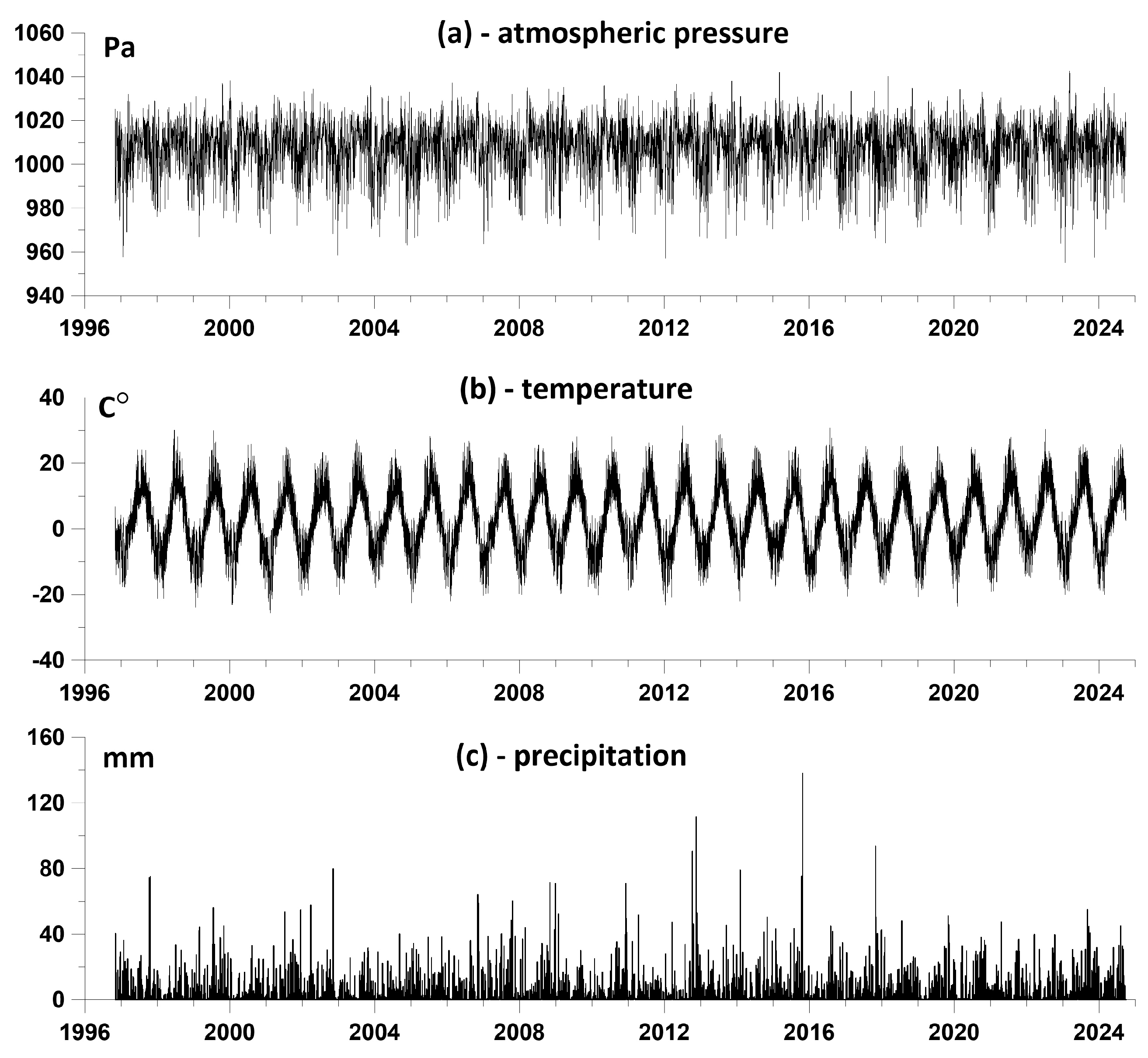
Figure 2.
Map of epicenters of 418 earthquakes with that occurred in the KB GS RAS responsibility area (area bounded by the red line) from November 4, 1996 to September 30, 2024, and the location of the Pionerskaya weather station (black circle). Red lines are active faults according to [16].
Figure 2.
Map of epicenters of 418 earthquakes with that occurred in the KB GS RAS responsibility area (area bounded by the red line) from November 4, 1996 to September 30, 2024, and the location of the Pionerskaya weather station (black circle). Red lines are active faults according to [16].
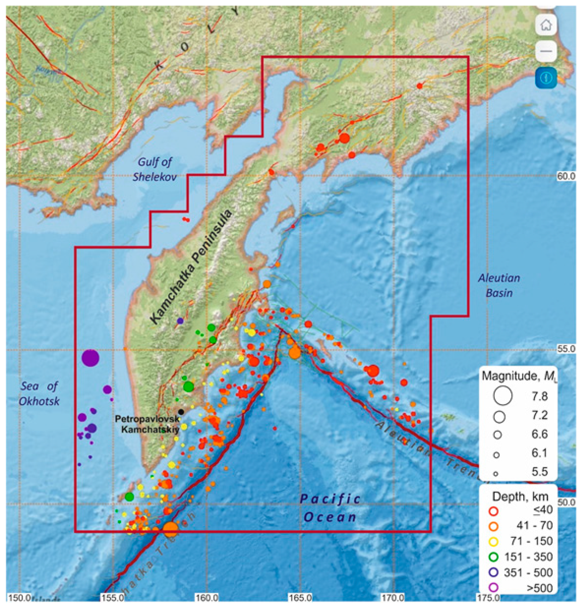
Figure 3.
Waveforms of the EEMD decomposition of the atmospheric pressure series for IMF levels with numbers from 1 to 12, the amplitudes of their envelopes and instantaneous frequencies calculated using the Hilbert transform.
Figure 3.
Waveforms of the EEMD decomposition of the atmospheric pressure series for IMF levels with numbers from 1 to 12, the amplitudes of their envelopes and instantaneous frequencies calculated using the Hilbert transform.
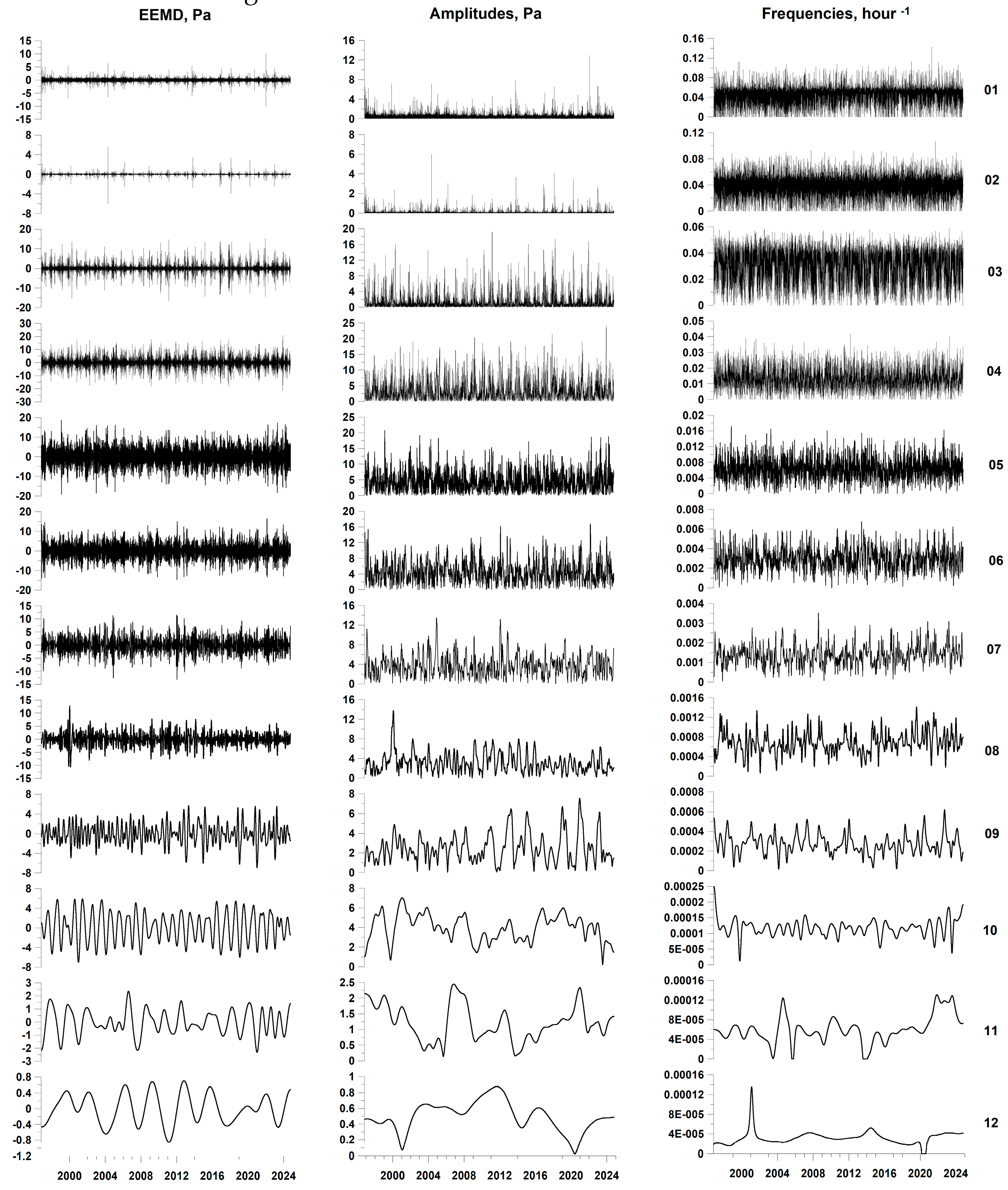
Figure 4.
Waveforms of the EEMD decomposition of the air temperature series for IMF levels with numbers from 1 to 12, the amplitudes of their envelopes and instantaneous frequencies calculated using the Hilbert transform.
Figure 4.
Waveforms of the EEMD decomposition of the air temperature series for IMF levels with numbers from 1 to 12, the amplitudes of their envelopes and instantaneous frequencies calculated using the Hilbert transform.
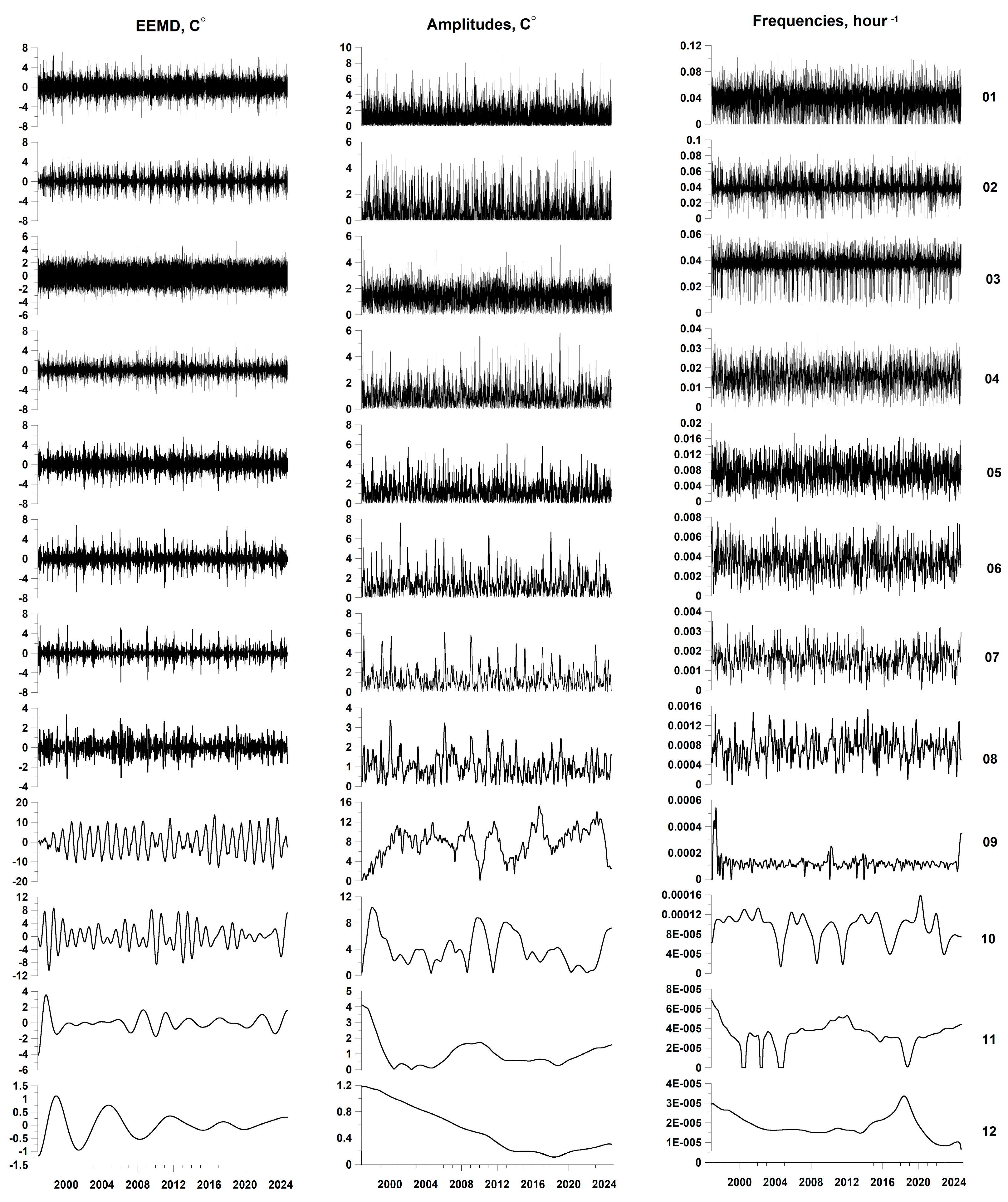
Figure 5.
Waveforms of the EEMD decomposition of the precipitation series for IMF levels with numbers from 1 to 12, the amplitudes of their envelopes and instantaneous frequencies calculated using the Hilbert transform.
Figure 5.
Waveforms of the EEMD decomposition of the precipitation series for IMF levels with numbers from 1 to 12, the amplitudes of their envelopes and instantaneous frequencies calculated using the Hilbert transform.
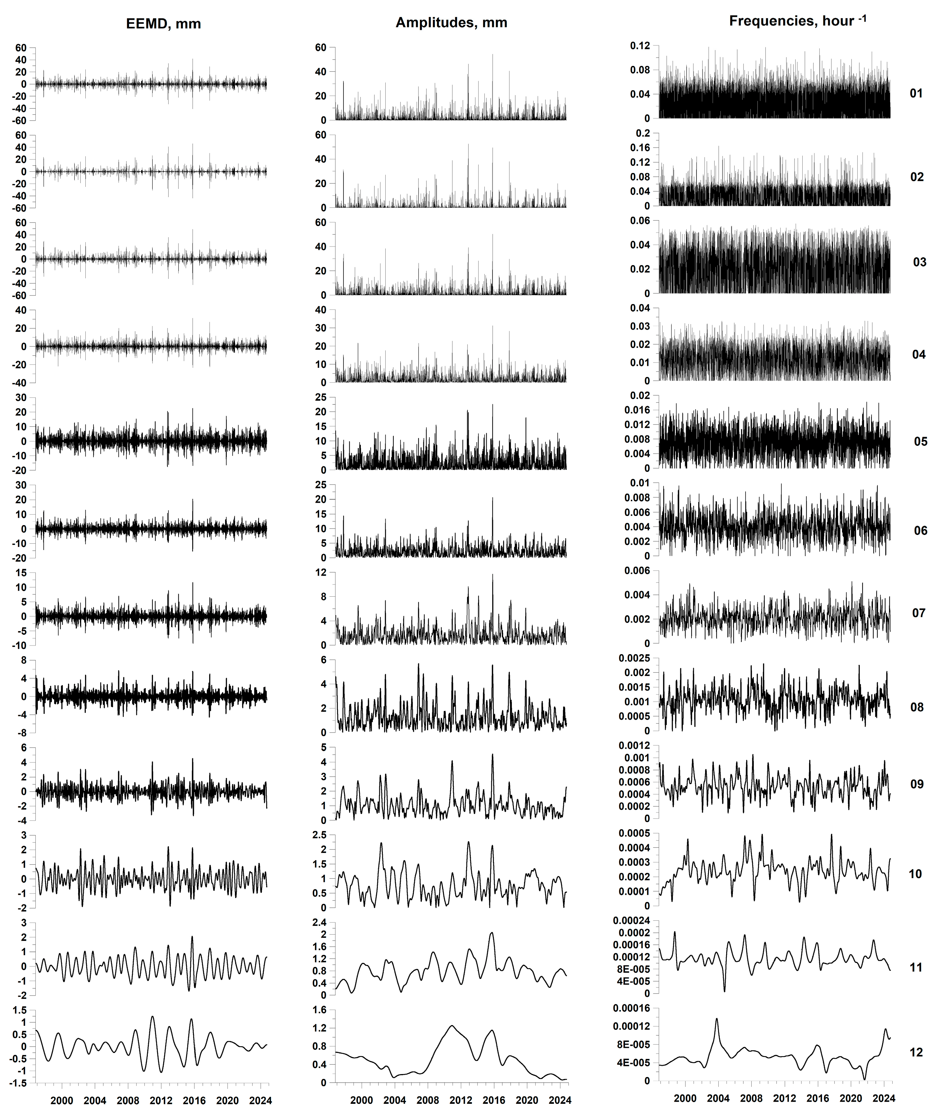
Figure 6.
Average values of instantaneous frequencies depending on the IMF level number for time series of atmospheric pressure (blue), air temperature (red) and precipitation (green).
Figure 6.
Average values of instantaneous frequencies depending on the IMF level number for time series of atmospheric pressure (blue), air temperature (red) and precipitation (green).
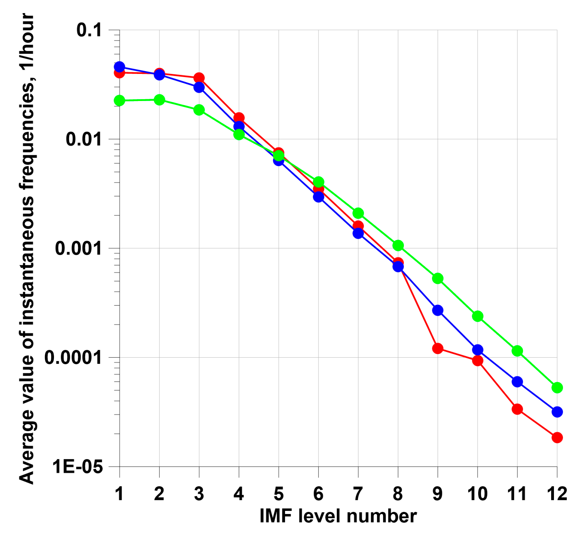
Figure 7.
(a) – time sequence of 418 earthquakes with magnitude ; (b, c, d, e) – results of calculating the amplitudes of the envelope for decompositions of the original time series: (b) – for the 6th IMF level of decomposition of the atmospheric pressure series; (c) – for the 6th IMF level of decomposition of the air temperature series; (d) – for the 6th IMF level of decomposition of the atmospheric precipitation series; (e) – for the 6th level of wavelet decomposition of the air temperature series. The positions of the 418 largest local maxima of the envelope amplitudes are marked with red dots on each graph.
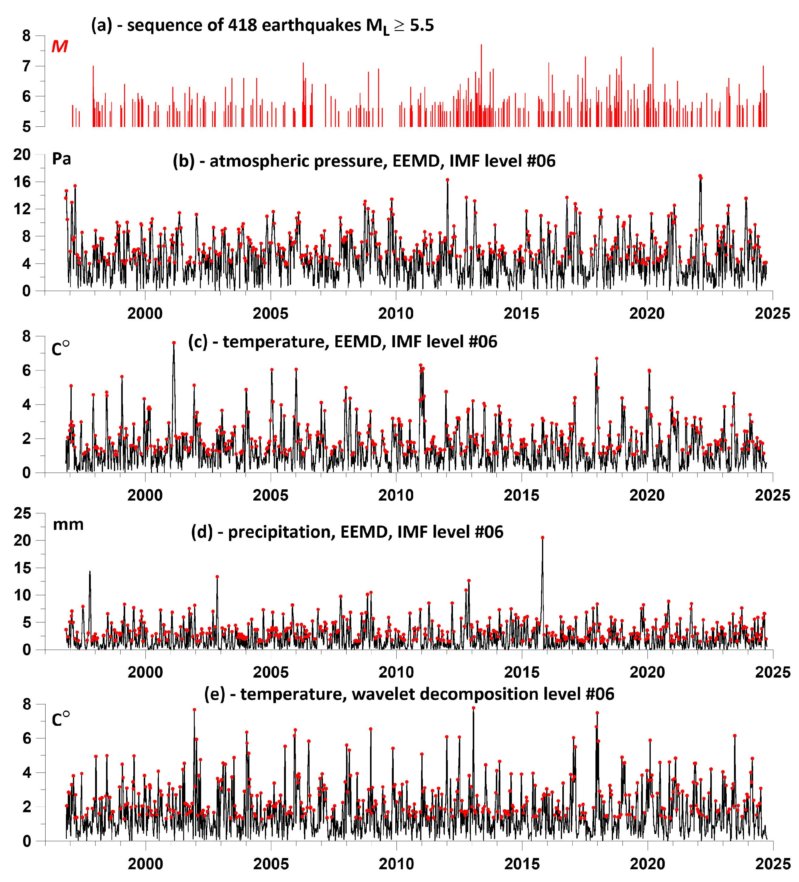
Figure 8.
Average values of the components of the influence matrices of the largest local maxima of the amplitudes of the envelopes of meteorological parameter series on seismic events (left column of the graphs) and average values of the components of the reverse influence (right column of the graphs). The horizontal red lines represent the average values of the averaged components of the influence matrices for each meteorological parameter for the "direct prognostic" (left column of the graphs) and "reverse postseismic" (right column of the graphs) influence. The values of the average values are shown in red above each horizontal mean line.
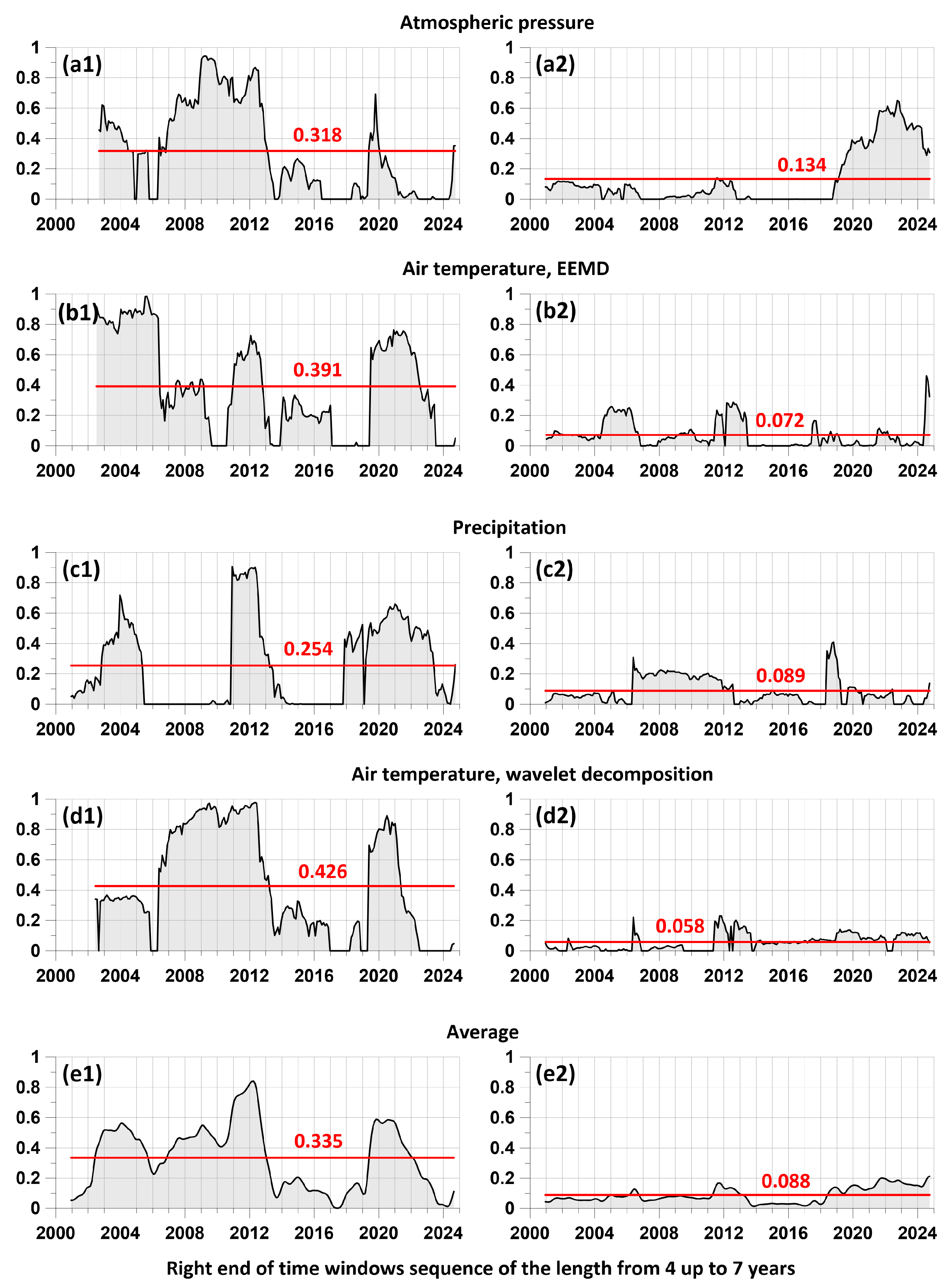
Figure 9.
Average values of the components of the matrices of the influence of the largest local maxima of the amplitudes of the envelopes of atmospheric pressure and air temperature series (the precipitation time series is excluded) on seismic events in comparison with the time moments of earthquakes with magnitudes (Figure 9(a)) and the closest earthquakes for which the ratio of the epicentral distance to the size of their source is (Figure 9(b)).
Disclaimer/Publisher’s Note: The statements, opinions and data contained in all publications are solely those of the individual author(s) and contributor(s) and not of MDPI and/or the editor(s). MDPI and/or the editor(s) disclaim responsibility for any injury to people or property resulting from any ideas, methods, instructions or products referred to in the content. |
© 2024 by the authors. Licensee MDPI, Basel, Switzerland. This article is an open access article distributed under the terms and conditions of the Creative Commons Attribution (CC BY) license (http://creativecommons.org/licenses/by/4.0/).
Copyright: This open access article is published under a Creative Commons CC BY 4.0 license, which permit the free download, distribution, and reuse, provided that the author and preprint are cited in any reuse.


