
Submitted:
07 August 2023
Posted:
08 August 2023
You are already at the latest version
Abstract
A method for studying properties of the earth's surface tremor, measured by means of GPS, is proposed. Four characteristics of tremor are considered: the entropy of the distribution of wavelet coefficients, the Donoho-Johnston wavelet index, and two estimates of the spectral slope. The anomalous areas of tremor are determined by estimating the probability densities of extreme values of the studied properties. The criteria for abnormal tremor behavior are based on the proximity to, or the difference between, tremor properties and white noise. The greatest deviation from the properties of white noise is characterized by entropy minima and spectral slope and DJ index maxima. This behavior of the tremor is called "active". The "passive" tremor behavior is characterized by the maximum proximity to the properties of white noise. The principal components approach provides weighted averaged density maps of these 2 variants of extreme distributions of parameters in a sliding time window of 3 years are considered. Singular points are the points of maximum average densities. The method is applied to the analysis of daily time series from a GPS network in the West USA in 2009-2022. It turned out that singular points of tremor form well-defined clusters.
Keywords:
GPS tremor singular points
; entropy
; spectral slope
; probability density
; principal components
1. Introduction
The spectral structure of the time series of displacements of the earth's surface, measured by means of space geodesy, is the subject of research by a large number of specialists. In [1,2,3,4] the maximum likelihood method was used to estimate the shape parameters of the power spectra and noise amplitude in different regions of the world. Errors in estimates of the displacement rate depending on the shape of the spectrum and on the intensity of the noise component of the time series were analyzed in [5,6,7]. Parametric models of GPS time series for the analysis of tectonically active areas were used in [8].
The structure of the high-frequency noise and low-frequency seasonal components of the GPS time series in connection with the problem of estimating the rates of displacement of tectonic plates was studied in [9,10,11,12]. Multivariate statistics methods (principal components, empirical orthogonal functions, and singular spectrum estimation) in [13,14] were used to identify common spatial and temporal components of the GPS time series. A joint analysis of the noise component of time series and accelerometer readings was carried out in [15]. Non-stationary effects were studied in [16,17,18] to assess the mutual motions of crustal blocks and station positioning stability.
The coherence of the earth's surface tremor was analyzed in [19,20]. In [21,22], fractal analysis of high-frequency GPS time series was used to assess seismic hazard in Japan and California.
This article presents a further development of the methods for analyzing the tremor of the earth's surface, proposed in [23], and analyzes the structure of high-frequency noise in the time series of the GPS station network in the Western United States during the time interval 2009-2022. The US West is one of the most seismically active regions. A dense network of GPS stations makes it possible to study in detail the features of the earth's surface oscillations and try to compare them with known "spots" of seismic activity. Note that earlier in [24], a study was made of the properties of seismic noise in Southern California in comparison with the seismic regime.
2. Materials
GPS ground displacement data taken from the Nevada Geodetic Laboratory website at: http://geodesy.unr.edu/gps_timeseries/tenv3/IGS14/
These data represent displacements of the earth's surface in three orthogonal directions, which we will further denote as E, N and U (Up) for displacements in the west-east, north-south and vertical directions, with a time step of 1 day [25].
In what follows, we will consider a regular grid of 100×150 nodes, covering an area with latitude from 32.5°N to 51°N and longitude from 115°W to 128.5°W. Figure 1(a) shows the positions of GPS points for measuring displacements of the earth's surface. Figure 1(b) shows the distribution density of GPS stations obtained using the Gaussian kernel estimate [26] at the nodes of this regular grid with a smoothing radius of 0.25° (about 28 km).
We will consider estimates of the properties of GPS time series in a sliding time window 365 days long with a shift of 7 days. For each time window, operable stations are determined from the condition that the number of gaps in the considered time window does not exceed 5% of the time window length, that is, that this number is no more than 18 values. Missing values are filled in with "plausible" data, which are found from the value to the left and right of the missing time interval of the same length as the length of the gap [19]. Figure 2 shows a graph of the number of operational stations within a sliding time window of 365 days for 14 years of observations, 2009-2022.
3. Description of the time series statistics used
For each station in each time window, 4 surface tremor statistics are computed for the 3 ground displacement components.
Spectral exponent. Let be a finite sample of the GPS time series within a window of sample lengths . Denote by the estimate of the signal power spectrum , - a sequence of discrete values of frequencies with a step , , , , - a time step. Here is the minimum length, which is greater than or equal to the sample length : , the index in formula (6) varies up to due to the symmetry of the power spectrum of real signals with respect to the Nyquist frequency : . We introduce the spectral exponent by the formula:
where period , the value is determined by the least squares method: , is a sequence of random variables with zero mean. In each time window, the power spectrum was computed after transition to increments using an autoregressive model (maximum entropy estimate) [27] with an autoregressive order of , i.e. 36 for a window of length 365 samples. The transition to increments before calculating the power spectrum aims to free from the dominant effect of low frequencies in the daily time series of GPS.
Wavelet-based entropy and wavelet-based spectral slope. The minimum normalized wavelet information entropy for the sample is determined by the formula:
Here denoted the coefficients of the orthogonal wavelet decomposition. Daubechies bases were used with the number of vanishing moments from 1 to 10 [28]. We chose such a basis from this set for which the value (2) is minimal for a given time window and for the considered component of the displacement of the earth's surface. By formula (2) .
After determining the optimal orthogonal wavelet, the wavelet power spectrum can be calculated as the average values of the squares of the wavelet coefficients at each level of detail of the decomposition:
In formula (3) are the wavelet coefficients at the detail level with number , index , where is the number of wavelet coefficients at the detail level with number , which corresponds to the frequency band with the central period [28]. The maximum detail level number is chosen such that it contains at least a given number of wavelet coefficients. Recall that the number of wavelet coefficients at the level of detail decreases by a factor of 2 when the level number increases by one. The value was used in the calculations, which gives the value for the window length . Values , are similar to conventional power spectra. The regression model is used to calculate the wavelet-based spectral slope:
where is a sequence of independent random variables with zero mean. The parameter in formula (4) is the wavelet-based spectral exponent, the value of which can be found by the least squares method: .
The threshold (5) separates rather large (informative) in their absolute values wavelet coefficients from other coefficients which are considered to be noisy. Thus, we can consider the dimensionless signal characteristics , , as the ratio of the number of the most informative wavelet coefficients, for which the inequality is satisfied, to the total number N of all wavelet coefficients.
The value in the formula (5) is the noise standard deviation estimate under the assumption that the noise is most concentrated in the 1st detail level of orthogonal wavelet decomposition. The estimate of standard deviation should be robust with respect to outliers in the values of the coefficients at the first level. To provide this, a median estimate of the standard deviation for a normal random variable is used:
For each station in each time window, 4 surface tremor statistics are computed for the 3 ground displacement components
where сk(1) are wavelet coefficients at the first level of detail; N/2 is the number of such coefficients. The estimate of the standard deviation σ from formula (6) determines the value (5) as a “natural” threshold for extracting noise wavelet coefficients. The quantity (5) is known in wavelet analysis as the Donoho–Johnstone threshold, and the expression for this quantity is based on the formula for the asymptotic probability of the maximum deviations of Gaussian white noise [28,29]. The DJ index values can be interpreted as a measure of the non-stationarity of seismic noise. For stationary Gaussian white noise, the index is zero. In [30,31,32] DJ-index was used as one of the main statistics for investigating properties of global low-frequency seismic noise.
Summarizing, we will briefly describe in the list the characteristics of the values of the tremor statistics for stationary white Gaussian noise, which is considered as a standard of a completely random oscillation:
1. The “usual” spectral exponent is the regression coefficient between the logarithm of the power spectrum values and the logarithm of the period (“spectral slope”). For white noise it is equal to zero (white noise has a “flat spectrum”).
2. Wavelet-based spectral exponent - the regression coefficient between the logarithm of the mean values of the squares of the wavelet coefficients for each level of detail and the logarithm of the period of the central frequency corresponding to the level of detail of the wavelet decomposition ("spectral slope"). For white noise is zero.
3. Donoho-Johnstone threshold (DJ-index) - the ratio of the number of "large" in absolute magnitude orthogonal wavelet coefficients to the total number of coefficients. For white noise is zero.
4. Minimum entropy of the distribution of squared orthogonal wavelet coefficients in the enumeration of wavelet basis functions in the class of Daubechies wavelets with the number of vanishing moments from 1 to 10. For white noise, the entropy is maximum.
Since we use 4 statistics for 3 components of the ground displacement vector, we get 12 statistics for each type of tremor. Let's put them in one matrix:
On the left side of the matrix (7) there are the designations of the characteristics of active tremor, on the right side of the matrix (7) there are the designations of the characteristics of passive tremor. Recall that we are considering a regular grid of nodes with a size of 100 nodes in longitude and 150 nodes in latitude. For each time window with a length of 365 days with a shift of 7 days, the values of all 12 sequences of the distribution of tremor properties at the nodes of the regular grid are determined.
4. Extreme value probability density maps
Let there be any value from the matrix (7), the estimates of which were obtained in a sliding time window. For each grid node and for each time window labeled at the right end of the window, we find the 10 closest seismic working stations, which gives 10 values of . Let's take their median value . The values form an "elementary" map corresponding to a time window of 365 days. Consider the values of the parameter as a function of two-dimensional vectors of longitudes and latitudes of nodes in an explicit form: . For each "elementary map" with a discrete time index , we find the coordinates of the nodes at which the extreme value is reached with respect to all other nodes of the regular grid.
As noted above, the choice of the minimum for entropies and the maximum for spectral slopes is due to the considerations that the anomalous regions of active tremor should be characterized by the values of statistics that reflect the maximum deviation from the properties of white noise. For passive tremor, the opposite is true: maxima for entropies and minima for spectral slopes. A cloud of two-dimensional vectors considered within a certain time interval forms a random set. Let us estimate their two-dimensional probability distribution function for each node of the regular grid. For this, the Parzen–Rosenblatt estimate with the Gaussian kernel function [26] will be applied:
Here, is the core averaging radius, are integer indices that enumerate the "elementary" maps of each time window. Thus, is the number of time windows in the considered time interval. The width of the smoothing band was used, which is approximately equal to 28 km.
In our analysis, time windows of 2 lengths are used: a “short” window of 365 days in length, which is used to obtain estimates of tremor parameters, and a “long” window of 1095 days (3 years) in length, in which a sequence of estimates of the distribution densities of extreme values of statistics is obtained tremor. Estimates of characteristics from matrix (7) are calculated using "short" time windows 365 days long. Next, the probability densities of extreme values are calculated from the values that fall within the current "long" time window of 1095 days, which are also shifted by 7 days. Each "long" window includes 105 "short" time windows.
As a result of such assessments, 24 maps of the distribution density of extreme values of tremor parameters were constructed, presented in Figure 3, on which 12 maps for active tremor are in the upper half, and 12 maps for passive tremor are in the lower half.
Purely visually, a high correlation of probability density maps of the distribution of extreme values of tremor statistics is noticeable, which suggests the use of the principal component method [33] to isolate the most common characteristics over space. In each "long" 3-year time window, we calculate a 12×12 correlation matrix between the probability densities of the distribution of extreme values of tremor statistics. Next, we determine the eigenvector corresponding to the maximum eigenvalue of the correlation matrix and use the squares of its components as weights to calculate the average weighted probability density in each “long” window. Next, we find the coordinates of the point that realizes the maximum average density. This sequence of operations performed in each "long" time window makes it possible to obtain the trajectory of geographic coordinates of points that realize the maximum values of the average probability density. These points are called singular tremor points.
The results of weighting the probability density maps of the distribution of extreme properties of tremor by the method of principal components are shown in Figure 4. On the map 4(a), red circles indicate the positions of singular points of active tremor, which are combined into 5 clusters. The clusters are numbered in descending order of the latitude of their centers of mass; the cluster numbers are also shown. On the map 4(b), blue circles indicate the positions of singular points of passive tremor, which form 3 clusters. On Figure 4(c) and 4(d) there are plots of histograms of the distribution of the number of singular points in each cluster for each type of tremor.
Figure 5 shows graphs of changes in the squares of the components of sequences of correlation matrices for probability density maps of the distribution of extreme values, respectively, for active (12 upper graphs) and passive (12 lower graphs). As noted above, these values are used as weight functions to obtain weighted average probability density maps. The result of such a weighing operation using the principal component method is shown in Figure 4. The graphs in Figure 5 show the average values of the weights calculated for all “long” time windows. For each tremor variant, 4 maximum average values of weights are highlighted in red - they select those components from matrix (7) that make the greatest contribution to obtaining the weighted average sum of probability densities.
The trajectories of changes in geographic latitudes and longitudes of singular points over time are shown in Figs. 6(a) and 6(b). Along the trajectories of change of coordinates there are marks of belonging to clusters of stations. Figure 6(c) shows how the distances between the singular points of active and passive tremor change as the sliding time window of 3 years moves from left to right. From this graph it can be seen that the concentration of singular points of both types of tremor in those regions where their positions are very close to each other, namely, cluster #2 of active singular points and cluster #1 of passive singular points mainly occurs in different time windows. The exception is the time intervals with labels of the right ends of the "long" 3-year windows 2012-2012.5 and 2015.5-2016, when the distances from singular points of different types are less than 100 km, but do not reach zero values. These temporal anomalies are of geodynamic interest, but their nature is still unclear.
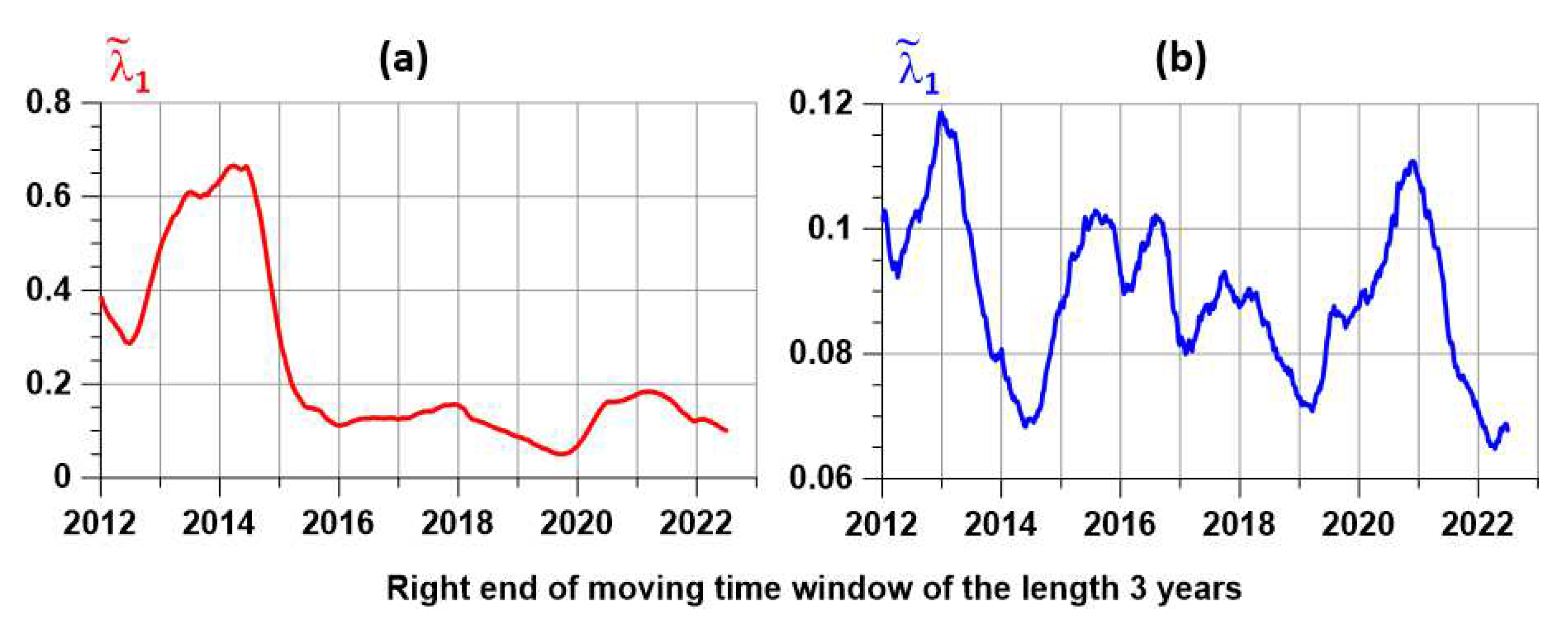
Denote by the normalized maximum eigenvalue of the correlation matrix:
In formula (9) are the eigenvalues of the correlation matrix, sorted in descending order: . According to the principal component method [33], the value is equal to the share of the total variance attributable to the first principal component and can be interpreted as a measure of synchronization of changes in the scalar components of the multivariate time series of the probability density values of the tremor statistics from the matrix in formula (7) in nodes regular grid covering the region under study.
Figure 7 shows graphs of changes in the eigenvalues of the correlation matrix for active and passive tremor. It can be seen from these plots that the active tremor (Figure 7(a)) is much more synchronized than the passive tremor (Figure 7(b)). Moreover, for active tremor, there is a very strong synchronization for the positions of the right end of the 3-year time window from 2013 to 2015. Given the length of the window, this synchronization takes a period of time from 2010 to 2015.
As was shown in [23,24], after a couple of the strongest earthquakes in the world, Maule in Chile on 2010.02.27 and Tohoku in Japan on 2011.11.03, there was an explosive increase in the radius of spatial correlations of global seismic noise properties. It is possible that the increase in synchronization of active tremor in the Western United States in 2010-2015. is also a response to this pair of mega earthquakes. Note that a sharp jump in the magnitude of global correlations of the earth's surface tremor in 2010-2011. was shown in [19], and [34] showed that before the 2011 Tohoku earthquake in Japan, long-term correlations arose between seismic noise in California and Japan.
Conclusions
A new method has been developed for studying the properties of the earth's surface tremor, measured by means of GPS, based on the use of oscillation statistics that describe the deviation or proximity to the properties of Gaussian white noise, considered as a standard of a stationary random signal. Based on the application of the principal component method to the estimation of the probability densities of the distribution of extreme properties of statistics in a sliding time window, new concepts of active and passive tremor and their singular points are introduced, and the trajectories of singular points are determined. The concept of tremor synchronization measure is introduced as the maximum eigenvalue of the correlation density matrix of distribution of extreme values of tremor statistics. The method is applied to the data of daily measurements of the earth's surface displacements on a network of GPS stations located in the Western United States during the time interval 2009-2022. It was shown that singular points of both types of tremor form well-defined clusters. Estimates of measures of synchronization of active and passive are given. A hypothesis has been put forward that strong synchronization of active tremor in 2010-2015. caused by a jump in the global synchronization of the tremor of the earth's surface and an explosive increase in the correlations of global seismic noise in 2010-2011.
Funding
This research received no external funding
Data Availability Statement
The open access data from the source: http://geodesy.unr.edu/gps_timeseries/tenv3/IGS14/ were used.
Acknowledgments
The work was carried out within the framework of the state assignment of the Institute of Physics of the Earth of the Russian Academy of Sciences (topic FMWU-2022-0018).
References
- Langbein, J.; Johnson, H. Correlated errors in geodetic time series, implications for time-dependent deformation. J. Geophys. Res. 1997, 102, 591–603. [Google Scholar] [CrossRef]
- Williams, S.D.P.; Bock, Y.; Fang, P.; Jamason, P.; Nikolaidis, R.M.; Prawirodirdjo, L.; Miller, M.; Johnson, D.J. Error analysis of continuous GPS time series, J. Geophys. Res. 2004, 109, B03412. [Google Scholar] [CrossRef]
- Bos, M.S.; Bastos, L.; Fernandes, R.M.S. The influence of seasonal signals on the estimation of the tectonic motion in short continuous GPS time-series. J. Geodyn. 2010, 49, 205–209. [Google Scholar] [CrossRef]
- Wang, W.; Zhao, B.; Wang, Q.; Yang, S. Noise analysis of continuous GPS coordinate time series for CMONOC. Adv. Space Res. 2012, 49, 943–956. [Google Scholar] [CrossRef]
- Caporali, A. Average strain rate in the Italian crust inferred from a permanent GPS network—I. Statistical analysis of the time-series of permanent GPS stations. Geophys. J. Int. 2003, 155, 241–253. [Google Scholar] [CrossRef]
- Zhang, J.; Bock, Y.; Johnson, H.; Fang, P.; Williams, S.; Genrich, J.; Wdowinski, S.; Behr, J. Southern California permanent GPS geodetic array: Error analysis of daily position estimates and site velocities. J. Geophys. Res. 1997, 102, 18035–18055. [Google Scholar] [CrossRef]
- Mao, A.; Harrison, C.G.A.; Dixon, T.H. Noise in GPS coordinate time series. J. Geophys. Res. 1999, 104, 2797–2816. [Google Scholar] [CrossRef]
- Li, J.; Miyashita, K.; Kato, T.; Miyazaki, S. GPS time series modeling by autoregressive moving average method, Application to the crustal deformation in central Japan. Earth Planets Space 2000, 52, 155–162. [Google Scholar] [CrossRef]
- Beavan, J. Noise properties of continuous GPS data from concrete pillar geodetic monuments in New Zealand and comparison with data from U.S. deep drilled braced monuments. J. Geophys. Res. 2005, 110, B08410. [Google Scholar] [CrossRef]
- Langbein, J. Noise in GPS displacement measurements from Southern California and Southern Nevada. J. Geophys. Res. 2008, 113, B05405. [Google Scholar] [CrossRef]
- Blewitt, G.; Lavallee, D. Effects of annual signal on geodetic velocity. J. Geophys. Res. 2002, 107, 2145. [Google Scholar] [CrossRef]
- Bos, M.S.; Bastos, L.; Fernandes, R.M.S. The influence of seasonal signals on the estimation of the tectonic motion in short continuous GPS time-series. J. Geodyn. 2010, 49, 205–209. [Google Scholar] [CrossRef]
- Teferle, F.N.; Williams, S.D.P.; Kierulf, H.P.; Bingley, R.M.; Plag, H.P. A continuous GPS coordinate time series analysis strategy for high-accuracy vertical land movements. Phys. Chem. Earth Parts A/B/C 2008, 33, 205–216. [Google Scholar] [CrossRef]
- Chen, Q.; van Dam, T.; Sneeuw, N.; Collilieux, X.; Weigelt, M.; Rebischung, P. Singular spectrum analysis for modeling seasonal signals from GPS time series. J. Geodyn. 2013, 72, 25–35. [Google Scholar] [CrossRef]
- Bock, Y.; Melgar, D.; Crowell, B.W. Real-Time Strong-Motion Broadband Displacements from Collocated GPS and Accelerometers. Bull. Seismol. Soc. Am. 2011, 101, 2904–2925. [Google Scholar] [CrossRef]
- Hackl, M.; Malservisi, R.; Hugentobler, U.; Jiang, Y. Velocity covariance in the presence of anisotropic time correlated noise and transient events in GPS time series. J. Geodyn. 2013, 72, 36–45. [Google Scholar] [CrossRef]
- Goudarzi, M.A.; Cocard, M.; Santerre, R.; Woldai, T. GPS interactive time series analysis software. GPS Solut. 2013, 17, 595–603. [Google Scholar] [CrossRef]
- Khelif, S.; Kahlouche, S.; Belbachir, M.F. Analysis of position time series of GPS-DORIS co-located stations. Int. J. Appl. Earth Observ. Geoinf. 2013, 20, 67–76. [Google Scholar] [CrossRef]
- Lyubushin, A. Global coherence of GPS-measured high-frequency surface tremor motions. GPS Solut. 2018, 22, 116. [Google Scholar] [CrossRef]
- Lyubushin, A. Field of coherence of GPS-measured earth tremors. GPS Solut. 2019, 23, 120. [Google Scholar] [CrossRef]
- Filatov, D.M.; Lyubushin, A.A. Fractal analysis of GPS time series for early detection of disastrous seismic events. Phys. A 2017, 469, 718–730. [Google Scholar] [CrossRef]
- Filatov, D.M.; Lyubushin, A.A. Precursory Analysis of GPS Time Series for Seismic Hazard Assessment. Pure Appl. Geophys. 2019, 177, 509–530. [Google Scholar] [CrossRef]
- Lyubushin, A. Identification of Areas of Anomalous Tremor of the Earth's Surface on the Japanese Islands According to GPS Data. Appl. Sci. 2022, 12, 7297. [Google Scholar] [CrossRef]
- Lyubushin, A.A. Seismic Noise Wavelet-Based Entropy in Southern California. Journal of Seismology 2021, 25, 25–39. [Google Scholar] [CrossRef]
- Blewitt, G.; Hammond, W.C.; Kreemer, C. Harnessing the GPS data explosion for interdisciplinary science. Eos 2018, 99, 485. [Google Scholar] [CrossRef]
- Duda, R.O.; Hart, P.E.; Stork, D.G. Pattern Classification; Wiley: Hoboken, NJ, USA, 2000. [Google Scholar]
- Marple, S.L., Jr. Digital Spectral Analysis with Applications; Prentice-Hall, Inc.: Englewood Cliffs, NJ, USA, 1987. [Google Scholar]
- Mallat, S. A Wavelet Tour of Signal Processing, 2nd ed.; Academic Press: Cambridge, MA, USA, 1999. [Google Scholar]
- Donoho, D.L.; Johnstone, I.M. Adapting to unknown smoothness via wavelet shrinkage. J. Am. Stat. Assoc. 1995, 90, 1200–1224. [Google Scholar] [CrossRef]
- Lyubushin, A. Low-Frequency Seismic Noise Properties in the Japanese Islands. Entropy 2021, 23, 474. [Google Scholar] [CrossRef]
- Lyubushin, A. Investigation of the Global Seismic Noise Properties in Connection to Strong Earthquakes, Front. Earth Sci. 2022, 10, 905663. [Google Scholar] [CrossRef]
- Lyubushin, A. Spatial Correlations of Global Seismic Noise Properties. Applied Sciences 2023, 13, 6958. [Google Scholar] [CrossRef]
- Jolliffe, I.T. Principal Component Analysis; Springer: Berlin/Heidelberg, Germany, 1986. [Google Scholar]
- Lyubushin, A.A. Long-range coherence between seismic noise properties in Japan and California before and after Tohoku mega-earthquake. Acta Geodaetica et Geophysica 2017, 52, 467–478. [Google Scholar] [CrossRef]
Figure 1.
(a) - network of GPS stations in the US West, 2009-2022; (b) is the density of GPS stations, estimated using a Gaussian kernel with a smoothing radius of 0.25 degrees on a regular grid of nodes with a size of 100×150.
Figure 1.
(a) - network of GPS stations in the US West, 2009-2022; (b) is the density of GPS stations, estimated using a Gaussian kernel with a smoothing radius of 0.25 degrees on a regular grid of nodes with a size of 100×150.
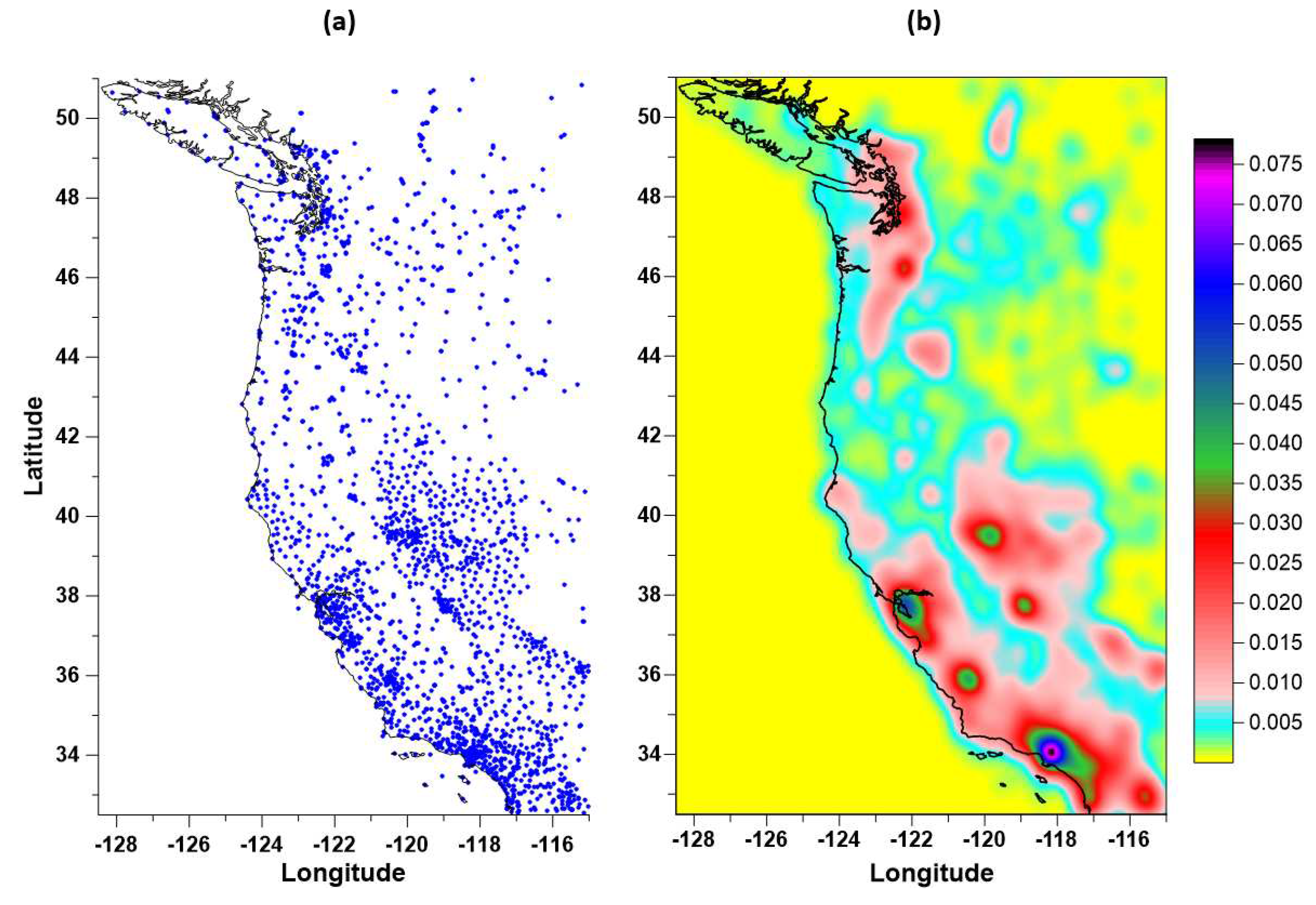
Figure 2.
The number of operational GPS stations in a 365-day window with a 7-day offset.
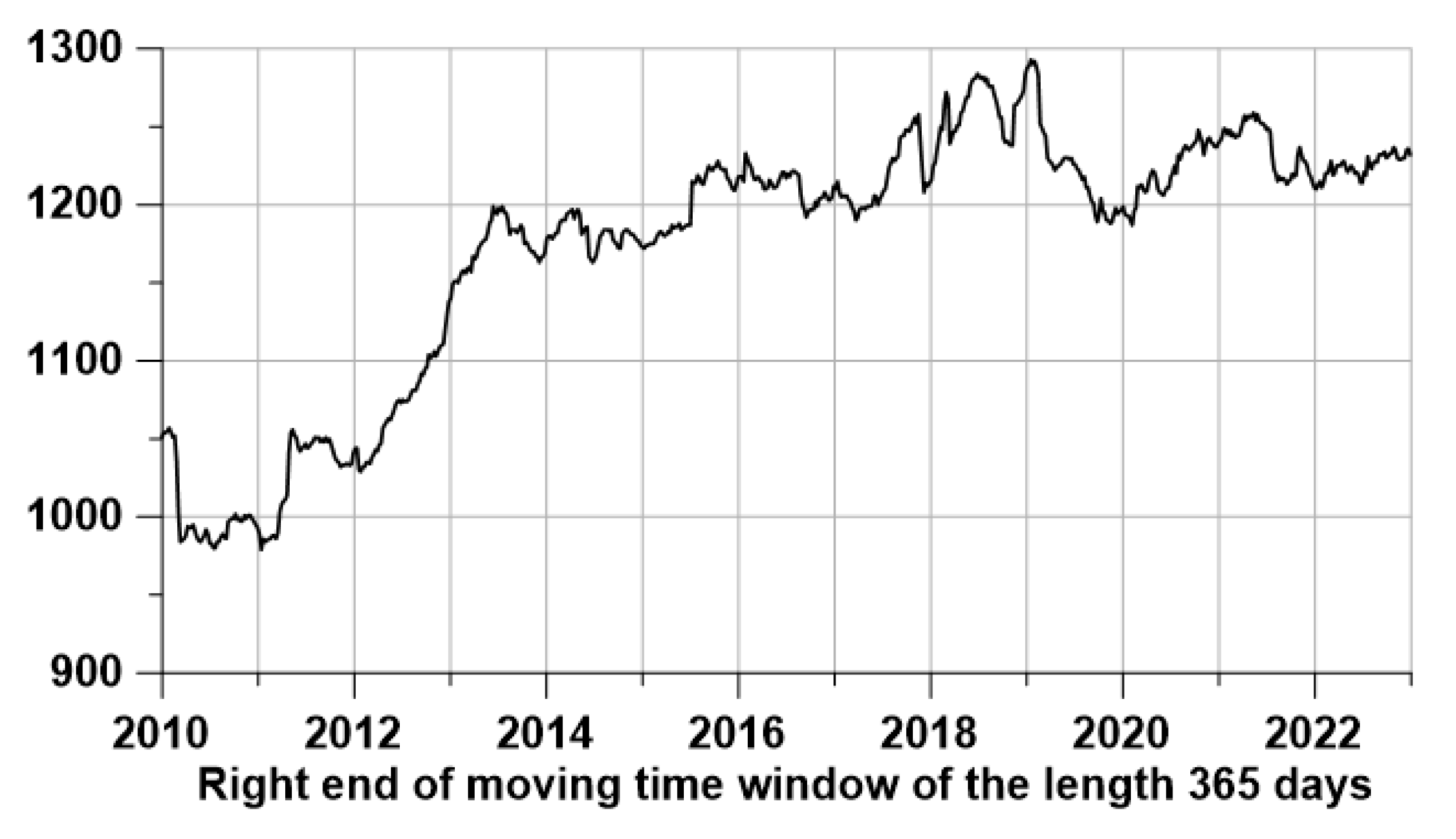
Figure 3.
Average probability densities of distribution of extreme values of 4 statistics of "active" and "passive" tremor of the earth's surface for 3 components of the displacement vector. Because each property value is estimated over a 365-day window offset by 7 days, the average probability density estimate is obtained by averaging 548 probability density maps, each derived from 105 tremor property value maps.
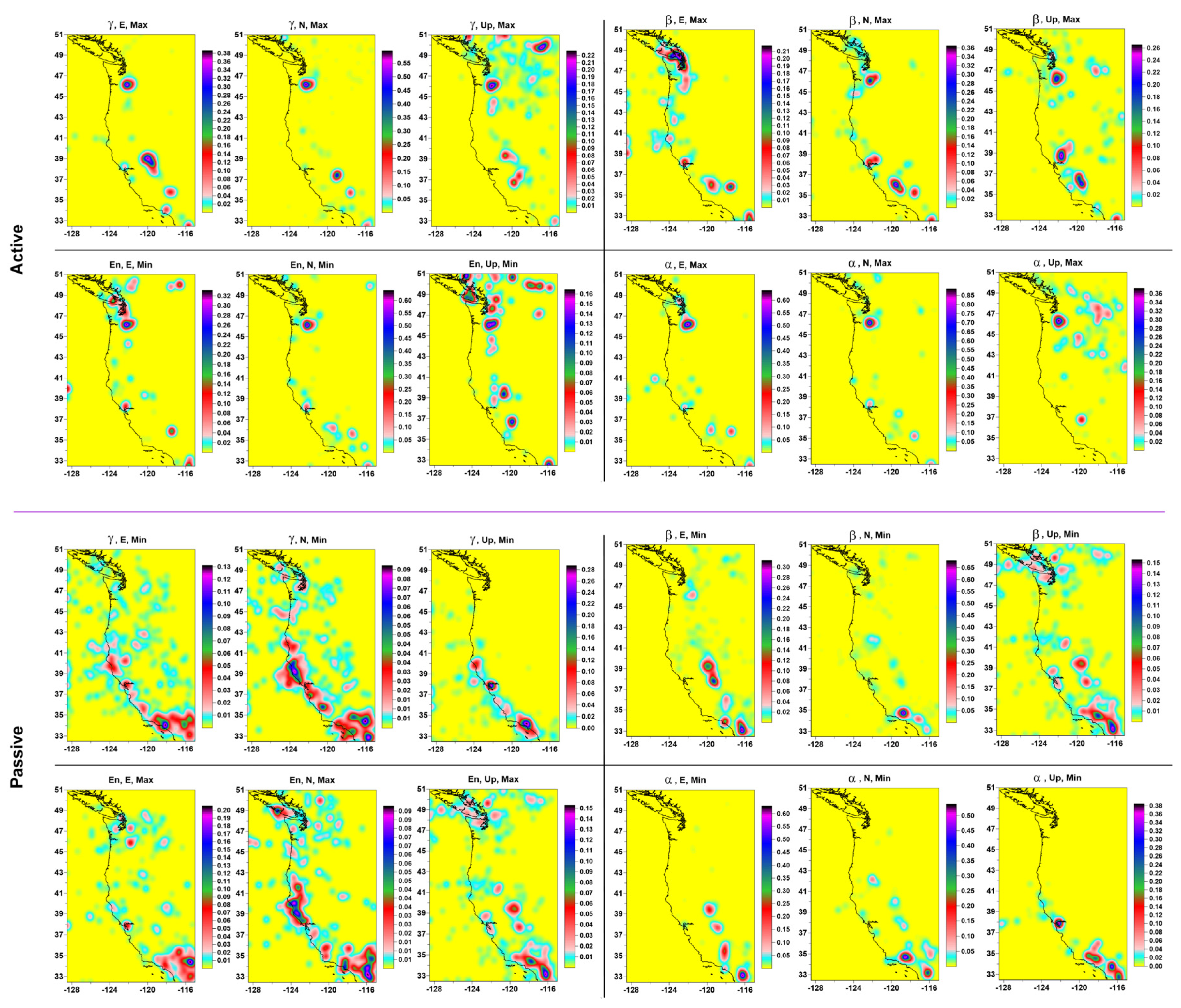
Figure 4.
Figure (4a) and (4b) are the results of averaging the weighted average probability densities of extreme values of 12 ground tremor statistics over a sliding time window of 3 years for active and passive tremor. The red circles in (a) represent the positions of active tremor singular points forming 6 numbered clusters, the blue circles in (b) represent the positions of passive tremor singular points forming 3 numbered clusters. Figure (4c) and (4d) are histograms of the numbers of singular points for "active" and "passive" tremors belonging to different clusters.
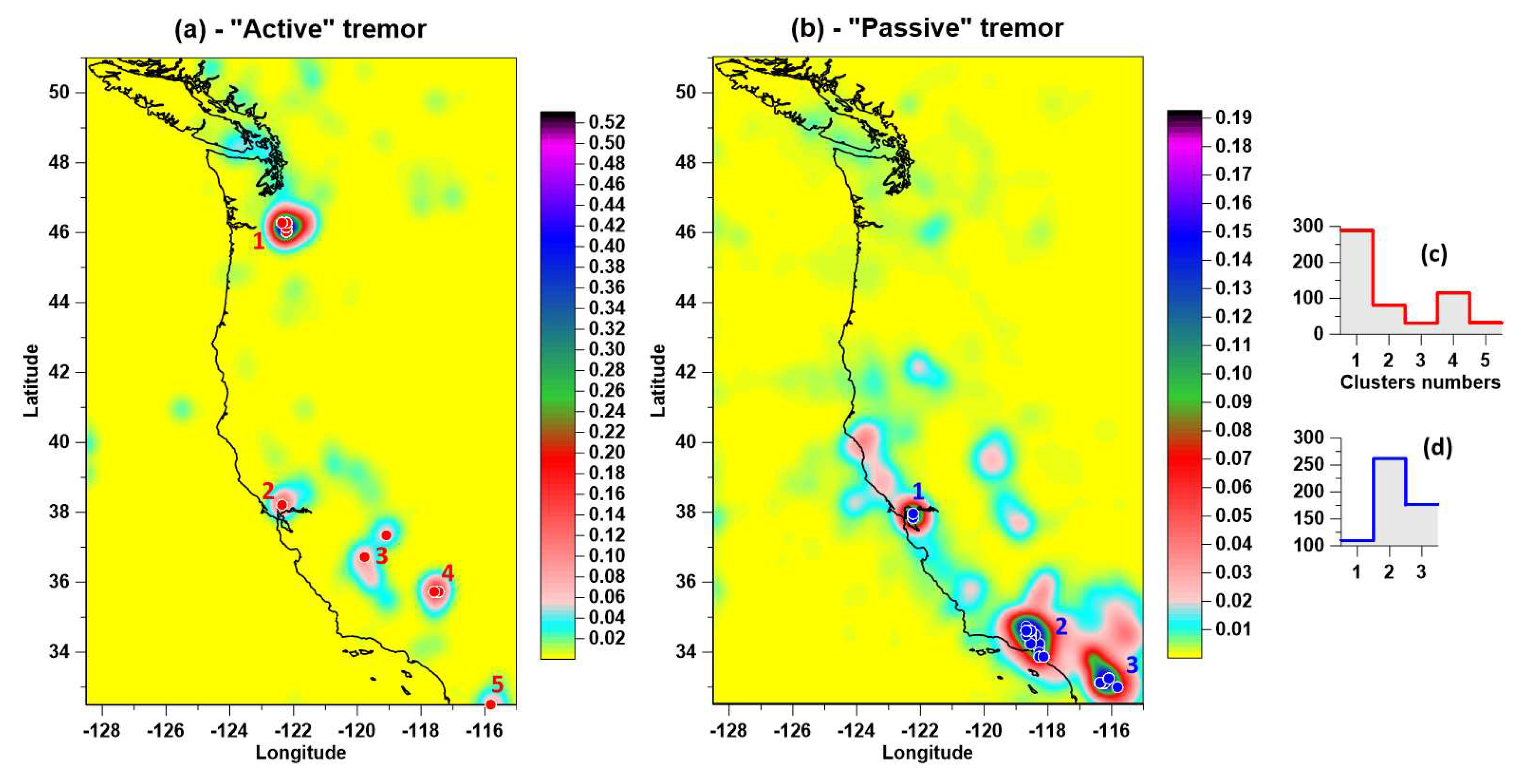
Figure 5.
Plots of changes in the weights of each of the 12 probability densities in "long" time windows of 1095 days with a shift of 7 days for "active" and "passive" tremor. The numbers indicate the average values of the weights, the 4 largest averages out of 12 variants for each type of tremor are highlighted in red.
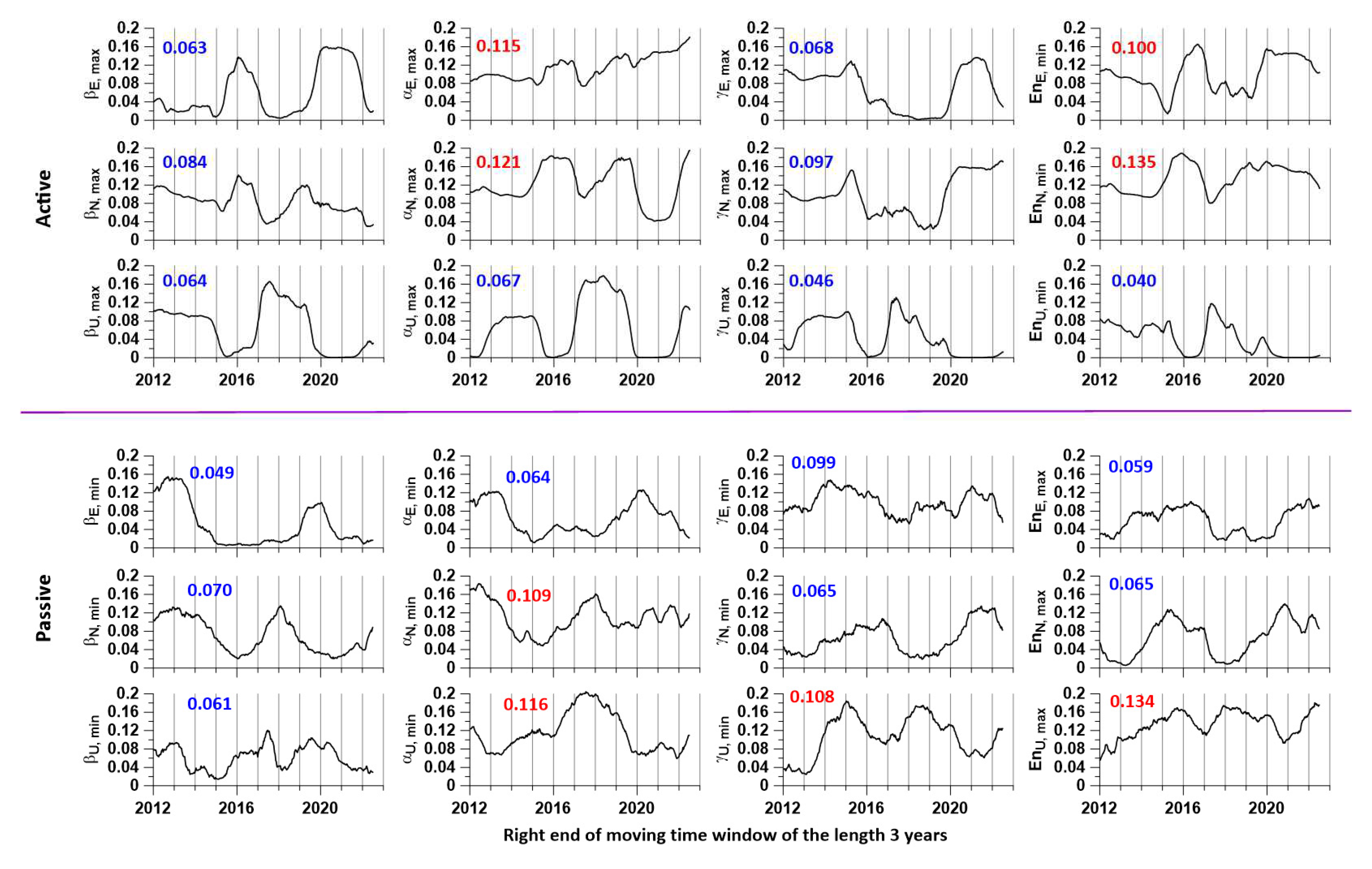
Figure 6.
Figure (6a) and (6b) - time sequences of longitudes and latitudes of singular points of tremor with a shift in the time window of 3 years for "active" (red) and "passive" (blue) tremor with cluster membership marks. Figure (6c) is the distance between the singular points of active and passive tremor in each time window of 3 years.

Figure 7.
Figure (7a) and (7b) - time sequences of values of the normalized maximum eigenvalue of the correlation matrix with a shift in the time window of 3 years for "active" (a) and "passive" (b) tremor.
Figure 7.
Figure (7a) and (7b) - time sequences of values of the normalized maximum eigenvalue of the correlation matrix with a shift in the time window of 3 years for "active" (a) and "passive" (b) tremor.
Disclaimer/Publisher’s Note: The statements, opinions and data contained in all publications are solely those of the individual author(s) and contributor(s) and not of MDPI and/or the editor(s). MDPI and/or the editor(s) disclaim responsibility for any injury to people or property resulting from any ideas, methods, instructions or products referred to in the content. |
© 2023 by the authors. Licensee MDPI, Basel, Switzerland. This article is an open access article distributed under the terms and conditions of the Creative Commons Attribution (CC BY) license (http://creativecommons.org/licenses/by/4.0/).
Copyright: This open access article is published under a Creative Commons CC BY 4.0 license, which permit the free download, distribution, and reuse, provided that the author and preprint are cited in any reuse.


