
Submitted:
22 June 2023
Posted:
23 June 2023
You are already at the latest version
Abstract
Noise model selection criteria has a significant impact on identifying the stochastic noise proper-ties of any GNSS daily coordinate time series. The low-frequency random walk noise existing in these time series could lead to overestimation of the tectonic rate, so it is of great significance to accurately detect the random walk component. This study focuses on noise model estimation cri-terion (BIC_tp) derived from the AIC and the BIC by introducing 2π factors. It is more sensitive to abnormal steps (random jumps). Using observation data from 72 GNSS stations from 1992 to 2022 and simulated data, four combined noise models are used to explore the impacts of time se-ries lengths (ranging from2 to 24 years) and data loss (between 2% and 30%) on noise models and velocity estimation. The results show that as the time length increased, the selected optimal noise model, and the estimated uncertainty of the tectonic trend with different data gap, gradually con-verge. When the time length is short (less than 8 years), it could lead to the FNRWWN, FNWN, and PLWN models being mistakenly estimated as GGMWN models, thereby affecting the accura-cy of determining the station velocity parameters. When the time length is 12 years, the RW noise component is more probably detected, As the time length increases, the impact of RW on velocity uncertainty is weakened. Finally, we conclude that for a time series with a minimum time length of 12 years, both the selection of the optimal stochastic noise model and the estimation of the ve-locity parameters are reliable.
Keywords:
GNSS time series
; time length
; missing data
; noise analysis
; velocity estimation
1. Introduction
The continuous operation of global navigation satellite system (GNSS) stations for over 20 years has provided valuable data that has been fundamental for geodesy and geodynamics research. GNSS has seen tremendous advances in the precision of the measurements, which allow researchers to study geophysical [1], plate tectonic [2,3,4] and post-glacial rebound [5], crustal deformation [6], landslide movement [7], ground subsidence [8], sea level change [9,10,11,12], or environmental loading [13].
Furthermore, the velocity uncertainty of GNSS stations is directly related to the parameters of the noise model of the GNSS time series. Selecting the optimal noise model is a key to obtain a reliable velocity estimate and associated uncertainty [14,15]. An inappropriate noise model could bias the estimation of this parameter, which could then affect the results of GNSS in high-precision geodynamics studies [16,17]. The study of the noise characteristics of a GNSS time series is of great important for GNSS velocity and uncertainty estimations.
Currently, the optimal stochastic noise model of a GNSS coordinate time series is generally chosen as a flicker noise and white noise (FNWN) [18,19,20,21]. Li et al. [22] analyzed the noise characteristics of 11 international GNSS service (IGS)stations in mainland China, and the results showed that the diversity of the noise models included FNWN, flicker noise and random walk noise and white noise (FNRWWN), power law noise and white noise (PLWN), and first-order Gauss–Markov noise (FOGM) noises. It has been demonstrated that the noise associated with GNSS time series can be characterized as WN plus colored noise. The colored noise is generally modeled as a PLWN [23] including the FN noise, the RW noise, and generalized Gauss–Markov and white noise (GGMWN). FN and RW are special case of the power-law noise following [24,25]. He et al. [26] studied 110 IGS stations and found that when observed over a time length of at least 12 years, they identified the presence of RW, which increased the uncertainty of the linear trend by a factor from approximately 1.5 to 8.4 depending on the selected stochastic noise model. However, the actual noise characteristics of the GNSS station are more complicated. With the continuous accumulation of the GNSS data, the long-period noise components (e.g., RW) could become more important, which then provide favorable conditions for detecting their existence. Regarding the identification of the noise model for a GNSS time series, most scientists have adopted the power spectrum analysis method and the maximum likelihood estimate (MLE)method for noise model analysis [27]. The power spectrum analysis method can provide a qualitative estimate of the noise model, but its resolution for low-frequency noise (e.g., RW noise) is low. The MLE method accurately estimate the characteristic parameters of the noise model However when the number of model parameters increases, the results show a significant bias. To overcome the shortcomings of the MLE method, Akaike [28] proposed noise-model-estimation criteria based on Akaike information criteria (AIC) and Bayesian information criteria (BIC) [29].
Bos et al. [30] proposed using AIC or BIC values to select relatively better noise models. Amiri-Simkooei et al. [31,32]. proposed a W-test method to select the optimal noise model. The AIC/BIC model estimation criteria improve the accuracy and the efficiency of noise model selection, to some extent. However, when the complexity of the model increases, the model selected by the AIC does not converge to a true model. BIC displays a similar weakness especially with the GGM model. Moreover, this method has shown certain divergent properties [14]. Here, we use the BIC true positives (BIC_tp) in order to select the optimal noise model.
Moreover, missing data is a persistent issue in the analysis of the GNSS station coordinate time series. Missing data can disrupt the continuity and the integrity of the time series, which has the potential of biasing the estimated model parameters. It is necessary to investigate the effects of the data gaps on the noise model and velocity estimation.
This paper is organized as follows: Section 2 describes the data and noise models and the selection criteria (including AIC, BIC, and the new BIC_tp). Section 3 shows the results varying the time length and the length of the data gap in the model selection and the estimation of stochastic noise parameters. Section 3 discusses the influence of time length and missing data on the noise model. Section 4 discusses the influence of the velocity and the velocity uncertainty, due to the time length and missing data. Section 5 concludes this work.
2. Materials and Methods
2.1. Data
2.1.1. GNSS Time Series
We analyzed analyze daily time series from 72 GNSS stations from the Enhanced Solid Earth Science ESDR System [33,34], and the distribution of the selected 72 GNSS stations is shown in Figure 1. GIPSY software is used to solve the daily solution of GNSS data, and the inter-quartile-range (IQR) method is used to eliminate gross errors in the resultant time series in order to obtain a "clean" daily position coordinate time series. In addition, offsets could have a significant impact on the noise model. In this work, the offsets detection method is the automatic offset detection algorithm developed by Fernandes and Bos [2,3,35].
2.2.2. Simulation Time Series
The classic trajectory model is used to simulate the GNSS coordinate time series [36]:
where () is the observation time (unit: a); a and b are the starting position and the velocity of the observation station’s coordinate time series; c and d represent the annual motion of the station; e and f represent the semi-annual motion of the station; is the Heaviside step function; is the sudden change value at the time of earthquake occurrence; is the number of earthquakes that occurred (, have the same meaning); is the rate of change in the station’s velocity after earthquakes; is the magnitude of post-seismic relaxation or slip displacement at a specific time; is the relaxation time constant of the station after the earthquake, and is the observation error.
The simulated station time series range from 2 to 30 years (denoted in the following as 2a, 4a, 6a, 8a, 10a, 12a, 14a, 16a, 18a, 20a, 22a, 24a, 26a, 28a, 30a), with 100 stations simulated for each case. Various 30 year-long simulated time series are displayed in Figure 2 with different noise models.
2.2. Methods
Bos [35] propose an estimation method that combined the AIC and BIC (AIC/BIC) noise model to overcome the bias of MLE, where the larger the MLE value, the greater the bias. AIC and BIC are used to estimate the noise model, and the smaller the AIC and BIC values, the closer the corresponding model is to the true model [37].
Studies have shown that the model selected for the AIC noise model estimation could not converge to the true model, and the BIC could not accurately identify the GGM models due to a divergence. Based on these factors, we follow the work of He et al (2019) noise model estimation criteria [26].
where L is the likelihood function, n is the length of the time series, and k is the number of variables in the model, v is the number of model parameters, and F is the Fisher information matrix. More detailed information about the noise model estimation criteria can be obtained at He et al. in 2019 [26,38].
3. Results
3.1. Impact of Time Span and Missing Data on the Noise Model
3.1.1. Simulated Noise Model Estimation
Table 1 shows the noise model estimation results using the FNRWWN model. We find that BIC_tp is more sensitive to RW noise and more likely to identify RW noise in the time series, as compared to the other information criteria. The detection success rate reaches 95% when the time length is about 12 years, and when the time length is greater, the detection rate is close to 1.
Our analysis of the results for the FNWN model show that the accuracy is 100% for time lengths of 4 years and longer as shown in Table 1. In addition, when using the FNWN model, the probability of 0 is associated with finding the FNRWWN mode.
Regarding the analysis of the noise model estimation results for the GGMWN and PLWN simulated, Table 2 shows that when the estimation length is 12a, the BIC_tp noise model detection rate for both models is as high as 100%. At 2a, the GGMWN model is erroneously estimated as the FNRWWN model, but the probability of detecting it as the FNWN model is 0. When the time length is less than 12a, the PLWN noise model could also be misidentified as the FNRWWN or GGMWN models. However, when the time length is greater than or equal to 12a, the detection rate of the BIC_tp noise model is 1, demonstrating the accuracy of the BIC_tp model estimation. Considering the limitations of the measured GNSS observation data, especially for high-precision geodynamic research, it is not possible to provide longer time series. Therefore, studying time series with a time length great than 12a is recommended.
3.1.2. Effect of Missing Data on Noise Model
The duration of the GNSS time series has a significant impact on the noise model selection. When analyzing the GNSS time series, it is necessary to ensure the reliability of the data (e.g., no large gaps) [39,40,41]. To explore the impact of data gaps on the noise model selection and estimated velocity, we simulate 100 time series with various lengths as described in the previous section. Missing rate is set to 2%, 5%, 8%, 10%, 12%, 15%, 18%, 20%, 25%, and 30%. The FNRWWN, FNWN, GGMWN, and PLWN noise models used in the optimal noise model selection using BIC_tp. Figure 3 shows the results.
According to the distribution of the different noise models, as shown in Figure 3 under different missing rates and different lengths, we found that when the time length is 12 years, the detection rates of all the models reached 90% Note that the detection rate of the FNWN noise model is consistently higher than 99%for different lengths. The results agree with the analysis of Table 1 and support our conclusions that BIC_tp is the best criteria to detect the RW component.
Now, with a data gap of 2% and 5%, or at the opposite 25% and 30%, the detection result curves of the FNRWWN, FNWN, GGMWN, and FNWN noise models are similar. The detection rate of the FNRWWN noise model is about 90% at 12 years. The detection curve of the GGMWN model is similar to the detection curve of FNRWWN. The detection rate of the PLWN noise model increases from about 62% for a length of 2 years to about 100% for 12 years. The detection rate of the FNWN noise model is around 99%–100%, for different lengths. However, when the time length is greater than 12 years, the detection probability of the GGMWN and PLWN noise models increases to 100% and is stable. The detection probability of the FNRWWN noise model increases, reaching 100% for a of 30 years.
In conclusion, the missing data has little effect on the different noise models. We consider that when ensuring a, with a time series length greater than 12 years, the impact of missing data on the noise model is small, and the noise model remained stable. This also suggested that BIC_tp is more sensitive to RW noise and more likely to identify the RW noise in the time series compared to other criteria. When the time length is 12 years, the success rate of noise model detection reaches 90% or more, and when the time length is greater than 12 years, the detection rate approaches 1.
3.2. Impact of Length and Missing Data on the Noise Model of the GNSS Time Series
3.2.1. GNSS Time Span on Noise Model Estimation
Further discussion on the impact of noise models on real GNSS station coordinate time series at different time lengths is conducted. A total of 72 GNSS stations time lengths of 2–24 years (2a, 4a, 6a, 8a, 10a, 12a, 14a, 16a, 18a, 20a, 22a, 24a) are selected, and the optimal noise model estimation is performed using noise models together with the BIC_tp. Spatial Distribution of the noise models for the north component of the GNSS time series for different time period are shown in Figure 4.(Spatial Distribution of the noise models for the east component of the GNSS time series for different time period are shown in Figure A1,Spatial Distribution of the noise models for the up component of the GNSS time series for different time period are shown in Figure A2.)
Based on the distribution of the optimal noise models for different components and time lengths, as shown in Figure 4, we found that the optimal noise model is consistent spatially. In the north and east coordinates, when the time period is less than 6 years, the optimal noise model is predominantly FNWN, with a model detection rate of about 86%. When the time period is 12 years, the detection rate of the FNWN model decreased to about 61%, and the percentage of the FNRWWN and PLWN models increased by about 16.7% and 20.8%, respectively. For time periods from 20 to 24 years, only a few stations exhibited an optimal noise model of GGMWN. As the time length increased to 12 years, the percentage and the amplitude of RW increased, indicating that the long-period components of the noise, such as RW noise, became significant in GNSS time series. In the vertical component, the influence of the noise model is more significant than that in the other two components [42,43,44]. As the time period increased, the percentage of the FNWN model decreased, and the percentages of the GGMWN and PLWN models increased. When the time length is 12 years, the detection rates of the GGMWN and PLWN models are both about 38%, and only a few stations exhibited the characteristics of the FNRWWN model. In summary, large time lengths provided conditions for detecting the presence of low-frequency noise. The RW noise cannot be detected with short time series. Combined with the simulation results analysis, the noise characteristics of the GNSS time series could be estimated by using the BIC_tp noise model. Considering the limitations of actual GNSS observation data, using time series of more than 12 years could obtain more reliable noise model estimation results. Further statistical analysis of the optimal noise models for different components and time lengths of the stations is shown in Figure 5, variations of the selected noise model using various time series length for another 17 stations are shown in Figure A3.
According to our analysis, in the north and east components, about 61% and 64%(respectively) of the analyzed stations, showed gradually stable noise model characteristics after the time length exceed 8a. However, the noise model is unstable, and the obtained results had a significant divergence. The statistical results showed that for over 60% of the stations, with an increased time scale, the divergence is reduced after the time length exceeded 8a. When the time length exceeded 12a, about 70%, 71%, and 90% of the stations for the north, east, and vertical components, the optimal noise model characteristic region became stable. This observation on the selected noise models for all components showed that when the time length is less than 8a, the uncertainty of the noise model is large [45,46]. To obtain reliable noise model estimation results, it is recommended to use GNSS time series with a length greater than 12a.
3.2.2. Effect of GNSS Missing Data on Noise Model
To further explore the variation in the noise models of real GNSS stations with different missing rates and during time periods, we found through statistical analysis that when the time length is less than 12a, the optimal noise models of the stations tend to be divergent, and the optimal noise model characteristics of the stations during different time periods are not consistent [47]. When the time length is greater than 12a, the noise models of the time series components in the north, east, and vertical components tend to be stable. The evolution of the noise models with different missing rates and during different time periods, after 12a, are shown in Figure 6. Evolution of different noise models with various missing rates for the east component is shown in Figure A4. Evolution of different noise models with various missing rates for the vertical component is shown in Figure A5.
According to the evolution of the noise models with different missing rates and during different time lengths, as shown in Figure 6, we could conclude that in the north, east, and vertical components, the FNWN noise model gradually decreased and converged with increases in the time lengths when the missing rate is different. In the north component, the FNRWWN and PLWN noise models gradually increased and converged to about 20% with increases in the time lengths, and the individual stations showed the characteristics of the GGMWN noise model. After 12a, the noise model is relatively stable and did not change. The evolution of the noise models in the east component is consistent with those in the north component. However, in the vertical component, the GGMWN and PLWN noise models gradually increased and converged to about 20% and 40%, respectively, with increases in the time lengths, and only a few stations detected the characteristics of the FNRWWN noise model. However, the noise model remained stable with increased in the time lengths. In summary, it indicated that the influence of the missing data on the noise models of real GNSS is small with different missing rates, and the noise model tended to be stable, which verified our conclusions based on the simulation data. However, in the real station coordinate time series, when the time length is greater than 12a, the success rate for detecting the FNWN noise model in the north and east component is about 60%, and in the vertical component, it is as about 40%, and different noise models remain stable.
4. Discussion
4.1. Impact of Length and Missing data on the Velocity Estimation of Simulation Time
4.1.1. Simulated Time Span on Velocity Estimation
To analyze the relationship between time length and velocity estimation, a statistical analysis of the velocity estimation results of the four sets of simulated time series is conducted. Figure 7 shows the variations in the mean velocities of 100 simulated sequences, from which we found that the station velocities gradually converged with increases in the time lengths. More accurate velocity parameters could be obtained using long-term time series. When the time length is 4 years, the velocity changed abruptly, possibly due to incorrect velocity estimation. However, when the time length is greater than 12 years, the trend of improving velocity precision with increased time lengths is relatively small and gradually converged to zero. Combined with Table 1, we found that when the time length is 12 years, the RW noise is more easily detected and its influence on velocity uncertainty is weakened with increases in the time lengths.
To further investigate the influence of different noise models on station velocity estimation, the uncertainty of the velocity estimates for 4 groups of simulated sequences using different noise models are statistically analyzed. Figure 8 shows the change in velocity uncertainty for the FNWN simulated sequences (an average of 100 stations), and the comparative analysis results for 100 stations are shown in Table 3.
As shown in Figure 8, we found that as the time length increased, the velocity uncertainty tended to stabilize and gradually converge to about 0.2 mm/y. The trend of improving velocity accuracy with increasing time lengths gradually decreased. Combined with Table 3, we observed that for the simulated FNRWWN time series, when its noise characteristics are assumed to be FNWN noise, the real station velocity uncertainty ranged from 3.1 to 7.4 times (the statistical average of 100 stations is 5.3 times) that of the FNWN background noise model. This could lead to the overestimation of the station velocity uncertainty, and the adverse effects primarily manifested as unreliable station velocity parameters being used as reliable data. Moreover, the data could not meet the accuracy requirements and negatively influence high-precision GNSS applications. Similarly, when the simulated FNRWWN time series noise characteristics are assumed to be background noise, the real station velocity uncertainty is from 2.7 to 4.5 times (with a mean of 3.5 times) and from 2.4 to 2.7 times (with a mean of 2.5 times) that of the GGMWN and PLWN background noise models, respectively. Therefore, accurate identification of RW noise is extremely important [48,49].
Similarly, for the velocity estimation parameters of the simulated FNWN time series, as analyzed in Table 3, when the simulated FNWN time series noise characteristics are assumed to be RWFNWN noise, the impact on station velocity estimation is small. In 99 out of 100 stations, the same station velocity uncertainty is obtained, with only one station showing a small difference (with an uncertainty ratio of 0.6), indicating that the impact on the estimation results is small when the FNWN time series is incorrectly estimated as RWFNWN. In addition, Table 3 shows that when the noise characteristics of the simulated sequences (FNRWWN, FNWN, PLWN) are assumed to be GGMWN background noise, the actual station velocity uncertainty is 3.5, 1.9, and 5.2 times (100 stations, on average) the assumed GGMWN noise model. Therefore, especially when the time length is short (as mentioned earlier, less than 12a), it could lead to the FNRWWN, FNWN, and PLWN models being mistakenly estimated as the GGMWN model, thereby affecting the determination accuracy of the station velocity field parameters.
Based on the analysis of 100 sets of simulation results, as the time length exceeded 12a, the trend of improving velocity accuracy with increasing time lengths became relatively small and gradually converged to 0. According to previous research, the noise model had a significant impact on the uncertainty of velocity, especially when the velocity uncertainty is large.
4.1.2. Simulated Missing Data on Velocity Estimation
To analyze the impact of data loss on velocity estimation, 100 sets of simulated data across the FNRWWN, FNWN, GGMWN, and PLWN noise models are used to simulate different degrees of missing data, with missing rates set at 2%, 5%, 8%, 10%, 12%, 15%, 18%, 20%, 25%, and 30%. The mean velocity change curves with different missing rates are shown in Figure 9, and the velocity uncertainty distribution curves with different missing rates are shown in Figure 10.
From Figure 10, we found that at different missing rates, the speed gradually converged and improved with increases in the time lengths, and more accurate speed parameters could be obtained through long-term time series. The speed accuracy improvement under the FNRWWM noise model had been decreasing, gradually converging to zero; the speed accuracy improvement with the PLWN noise model had an increasing trend when the length is between 2a and 4a, and gradually decreased and converged when the length is greater than 4a, but when the missing rate is 25%, the improvement in speed accuracy had been decreasing. The speed distribution under the GGMWN and FNWN noise models had a relatively small trend of improvement with increases in the time lengths, gradually converging to zero.
Based on the different missing rates in Figure 10, we found that with increases in the time lengths, the trend of decreasing speed uncertainty became stable, gradually converging to 0.2mm/y. The trend of improving speed accuracy gradually decreased with increases in the time lengths, proving that with different missing rates, the impact of the missing data on station velocity is small, and the improvement in station velocity accuracy decreased, year over year.
4.2. Impact of Time Span and Missing Data on the Noise Model of GNSS Time
4.2.1. Change in Velocity Estimation due to Different Time Span in GNSS Time Series
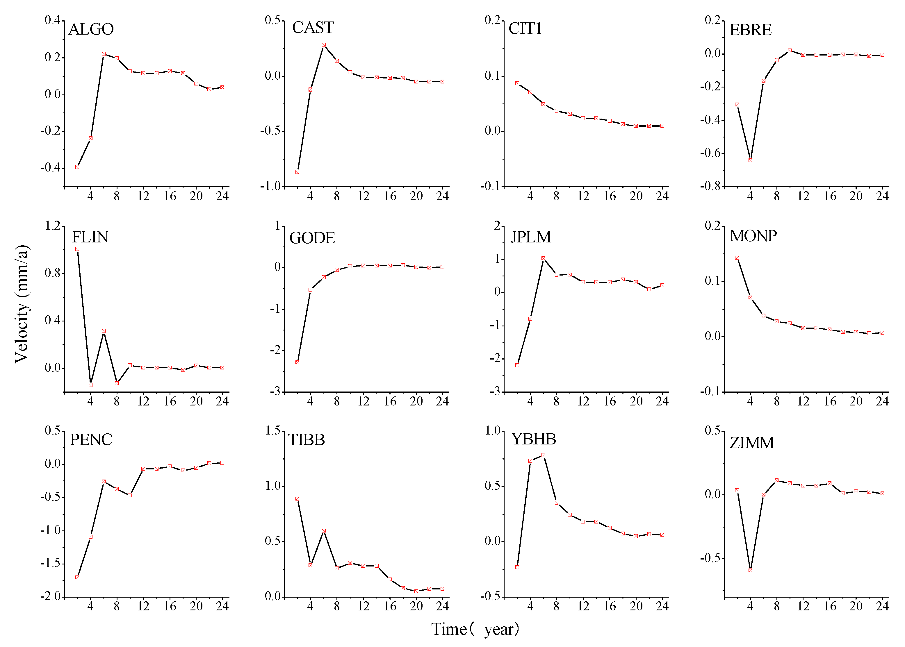
To analyze the impact of different time lengths on velocity and its uncertainty, the velocity and its uncertainty during different time lengths for 72 selected GNSS stations are analyzed, and Figure 11 show the distribution of the velocity evolution patterns (only 12 stations are selected due to space limitations). (Evolution of east component velocity law is shown in Figure A6. Evolution of vertical component velocity law is shown in Figure A7.)
Through the evolution of the speed changes over time in different components, as shown in Figure 11 we could conclude that when the time length is 6a and the noise model is in a non-stationary state, the estimated station velocity is larger. As the time length gradually increased (to 12a), the change in station velocity gradually decreased and tended to be stable, and the velocity estimate became more stable, consistent with the results estimated from the simulation data. In the north component, the anomalous YBHB station velocity decreased with increasing time lengths, and we observed that this station exhibited decreasing velocity in both the eastward and vertical components. The time series of this station showed the characteristics of the FNRWWN noise model. According to the SPOAC data, YBHB experienced a downward displacement of -8.319 mm in the vertical component during the 107-day period in 2011, with corresponding step changes in the eastward and northward components. Based on the evolution of the speed changes in the eastward component, as shown in Figure A6, we found that as the time length increased, after 12 years, most of the station velocity estimates became more stable, indicating that the velocity estimates are more reliable. The anomalous station MONP in the eastward component experienced a 21.278 mm displacement deformation during the 1994–2010 period, while the anomalous station TIBB experienced a displacement of 28.471 mm in the U component during the 1998 137-day period, followed by a coseismal deformation of 132.899 mm during the 1999 273-day period. The change in abnormal site speed could have been related to the site’s geographical environment (slow slip or earthquake) [50,51], and the velocity change is relatively large. The analysis of the evolution of the speed and the uncertainty of different components over time showed that as the length of the time series increased (after a time length of 12a), the estimated values of most station velocities tended to be stable and the velocity estimates became smaller, indicating that the velocity estimates are more reliable. The uncertainty of station velocity during different time periods for the 4 models is shown in Figure 12.
By analyzing the velocity uncertainty change curves of different models going in different components and during different time lengths, as shown in Figure 12, we found that the FNRWWN model had higher velocity uncertainty than the other 3 models and minimal station speed under the GGMWN noise model estimation [52,53], and the uncertainty values of the vertical estimated station velocity are larger. As the length of the time series increased, the uncertainty values of the velocity estimates decreased significantly, and the uncertainty of the velocity became more stable. In addition, the majority of the stations with high velocity uncertainty (e.g., MONP in the east component, YBHB in the north component, TIBB in the vertical component, etc.) had the optimal noise model of FNRWWN, indicating the presence of RW components, which led to unreliable velocity accuracy and large uncertainty. Therefore, in practical applications, further research is needed to reduce the impact of RW noise and improve the reliability of velocity for stations that show obvious RW components.
4.2.2. Effect of GNSS Missing data on Velocity Estimation
Comparing the real GNSS station coordinate time series over a length of 2–24 years, at intervals of 2 years, with the same missing rate as the simulated missing data rate, we explored the evolution of different component station velocities during different time lengths and with different missing rates. The northward different componential station velocities are taken as an example, as shown in Figure 13.
From the evolution rule of the station velocity during different time lengths and with missing rates in different components, as shown in Figure 13, we found that when the time length is between 6a and 10a, the station velocity increased with increases in the time lengths and with different missing rates. When the time length is between 10a and 16a, the station velocity decreased with increases in the time lengths. When the time length is greater than 16a, the station velocity showed an increasing trend with increases in the time lengths. To verify the reliability of the experimental results, further outlier detection is performed on the velocity differences. When the significance level is 0.05, we assumed that the velocity of the station with no missing data is equal to that of the station with missing data. The difference value is taken as the test variable, and the expected value of the difference value is 0, indicating that there is no abnormality in the velocity difference due to missing data. On the contrary, if the expected value is not 0, we considered that the velocity had changed significantly due to missing data. Based on this, taking the 24a long-term sequence in the north component as an example, a U-test [54] is introduced to compare the velocity difference between the station with no missing data and the station with missing rates from 2% to 30%. Compare the difference between the speed of stations that are not missing and those with a missing rate of 2% to 30%, and perform a U-test by using the residual speed of the two as the test variable, which is based on the principle in [54], as follows:
where is the velocity residual; is the standard deviation of the velocity residual; and is the standard statistic. The distribution of the velocity difference U-test with different missing rates in the north component is shown in Figure 14.
According to Figure 14, at the 0.05 significance level, the expected value of the velocity difference is 0, indicating that the velocity difference between the related non-missing data and the velocity with different missing rates is equal at a 95% confidence level, which indicated that the estimated velocity is not significantly affected by the missing rates. Further analysis of the velocity uncertainty with different missing rates is shown in Figure 15.
Based on Figure 15, we found that the accuracy of the station velocity gradually improved with increases in the time lengths. More accurate velocity parameters could be obtained through long-term time series. However, when the time length exceeded 12 years with different missing rates, the change in velocity uncertainty showed a decreasing trend and tended to stabilize, gradually converging to 0.2 mm/a, which verified the conclusion obtained from the simulation data.
In conclusion, when using the GNSS coordinate time series for high-precision geophysical applications, especially in the field of velocity, the corresponding time period of the obtained velocity field should be indicated, and time series longer than 12 years should be used as much as possible to weaken the influence of noise on the velocity and uncertainty in the coordinate time series. In addition, the velocity of the non-missing data is equal to that of the missing data at a 95% confidence level, and different missing rates had no significant effect on the estimation of velocity.
5. Conclusions
This study used 72 permanent GNSS time series, from 1998 to 2022, distributed globally. The improved BIC_tp is introduced to analyze the effects of different time lengths and data gaps on the noise model and station velocity. We conclude:
- The BIC_tp model had higher accuracy in estimating colored noise models and is sensitive to RW noise. By analyzing the simulated data and the real GNSS station coordinate time series noise models, we found that when the time length is greater than 12 years, the detection rate of the simulated data model is close to 1. Considering GNSS observation data, using time series greater than 12 years could obtain more reliable noise model estimation results, proving the accuracy of the BIC_tp model estimation.
- The time length had a significant impact on the noise model and station velocity estimation. With increases in the time lengths, the optimal noise model of GNSS coordinate time series, the estimated velocity together with associated uncertainty gradually converged (e.g., not much variability), and the percentage of RW noise model increased. We then recommend to use at least 12 years of GNSS data.
- Missing data had little effect on different noise models and could be considered as stable when the time series length is greater or equal to 12 years. Missing data did not change the selected noise model. With different data gaps and increasing time length, the velocity uncertainty does not change by approximately 0.2mm/a at around 12 years.
Author Contributions
X.S., X.H and J. P.M., writing-original draft preparation; S.H. and T.L., methodology, review, and editing; J.H., X.M., and Z.H., data processing and figure plotting. All authors have read and agreed to the published version of the manuscript.
Funding
This work is sponsored by Jiangxi Academic and Technical Leaders Training Program for Major Disciplines(20225BCJ23014), National Natural Science Foundation of China (42104023, 42061077,42064001),
Data Availability Statement
The processing of GNSS data can be obtained at http://garner.ucsd.edu/pub/measuresESESES_products.
Conflicts of Interest
The authors declare no conflict of interest.
Appendix A
Figure A1.
Spatial Distribution of the noise models for the east component of the GNSS time series for different time period.
Figure A1.
Spatial Distribution of the noise models for the east component of the GNSS time series for different time period.
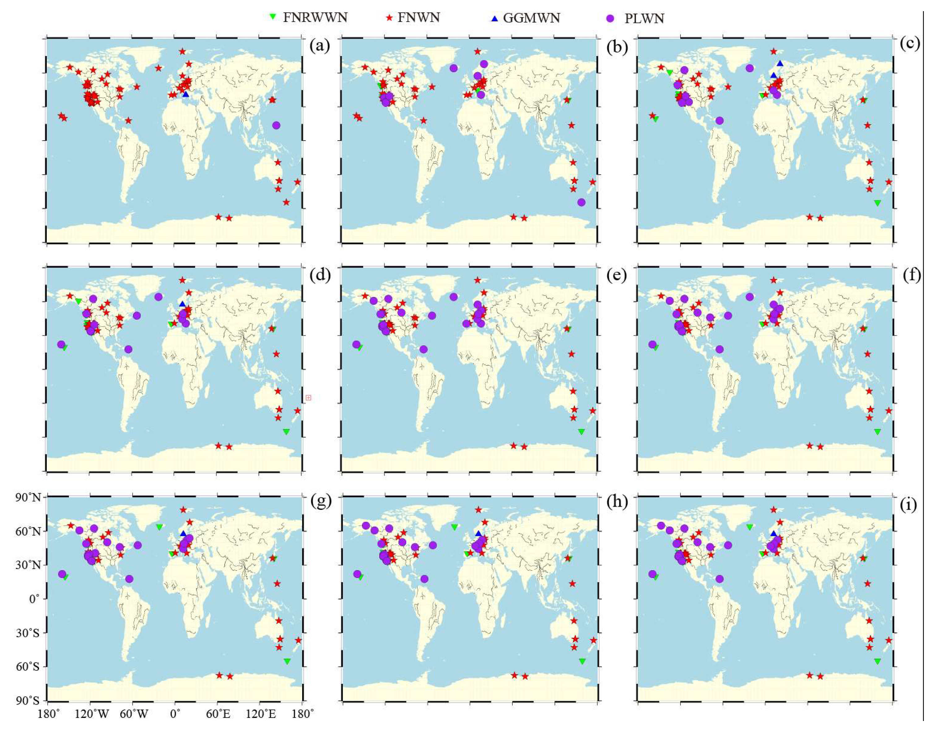
Figure A2.
Spatial Distribution of the noise models for the up component of the GNSS time series for different time period.
Figure A2.
Spatial Distribution of the noise models for the up component of the GNSS time series for different time period.
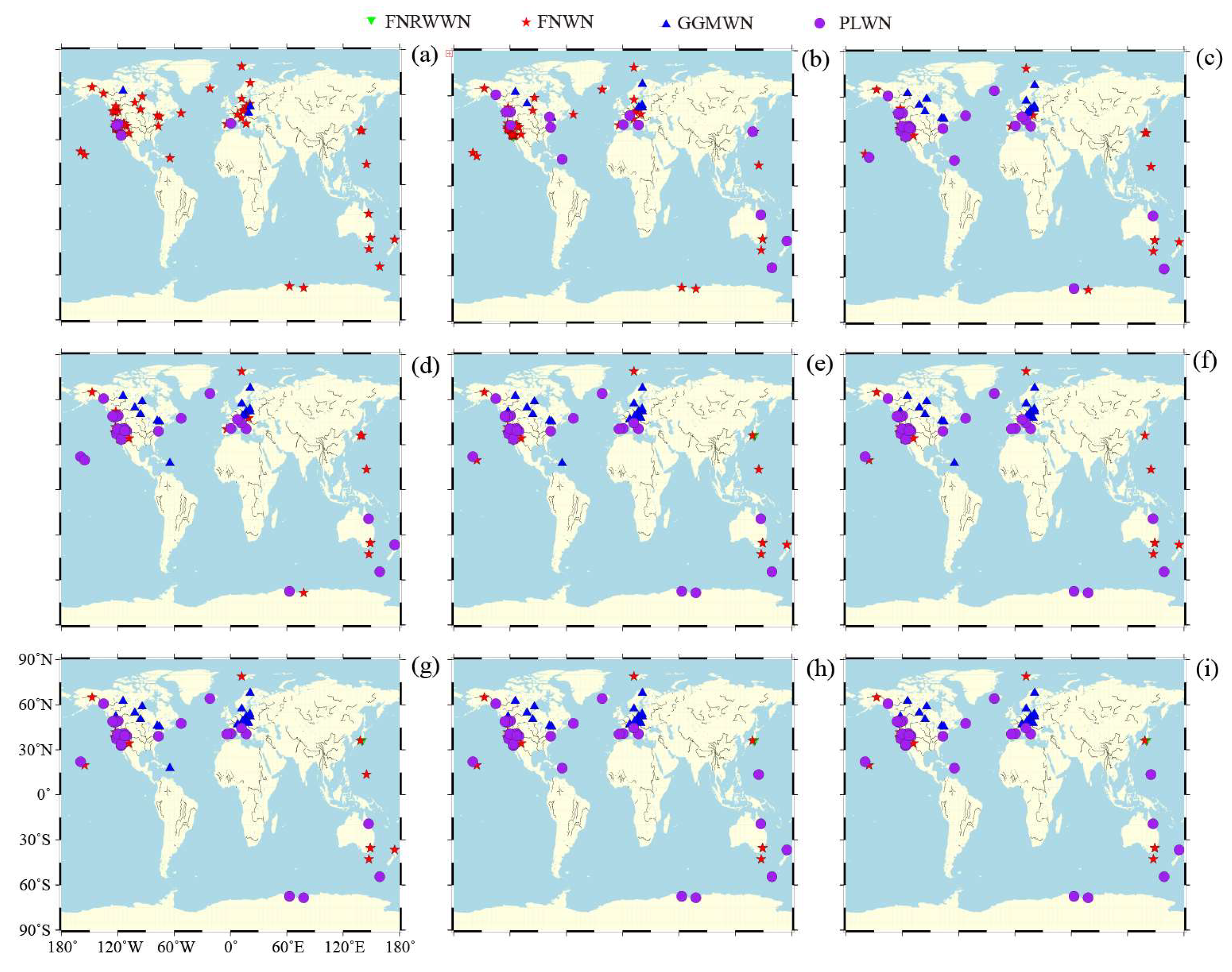
Figure A3.
Variations of the selected noise model using various time series length for another 17 stations are shown in Figure.
Figure A3.
Variations of the selected noise model using various time series length for another 17 stations are shown in Figure.
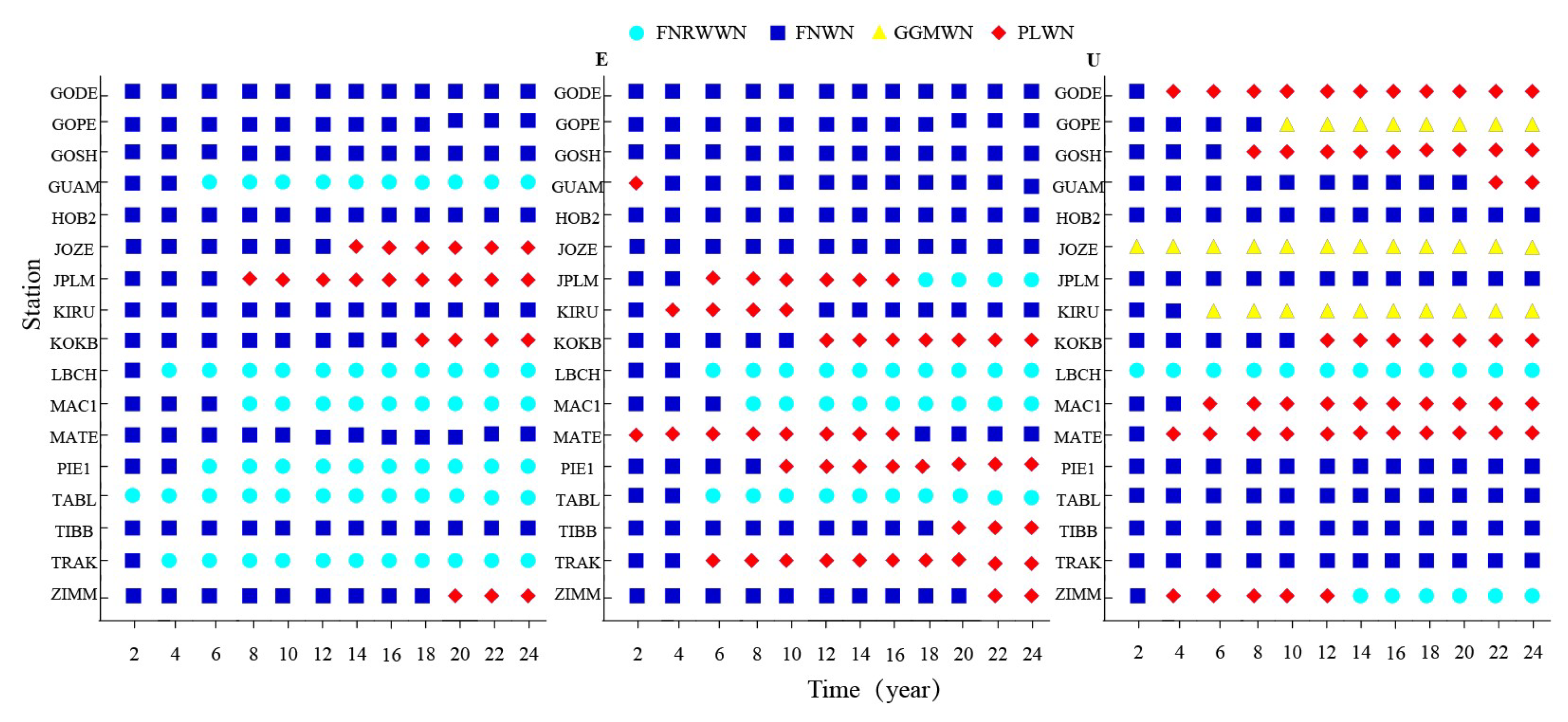
Figure A4.
Evolution of different noise models with various missing rates for the east component.
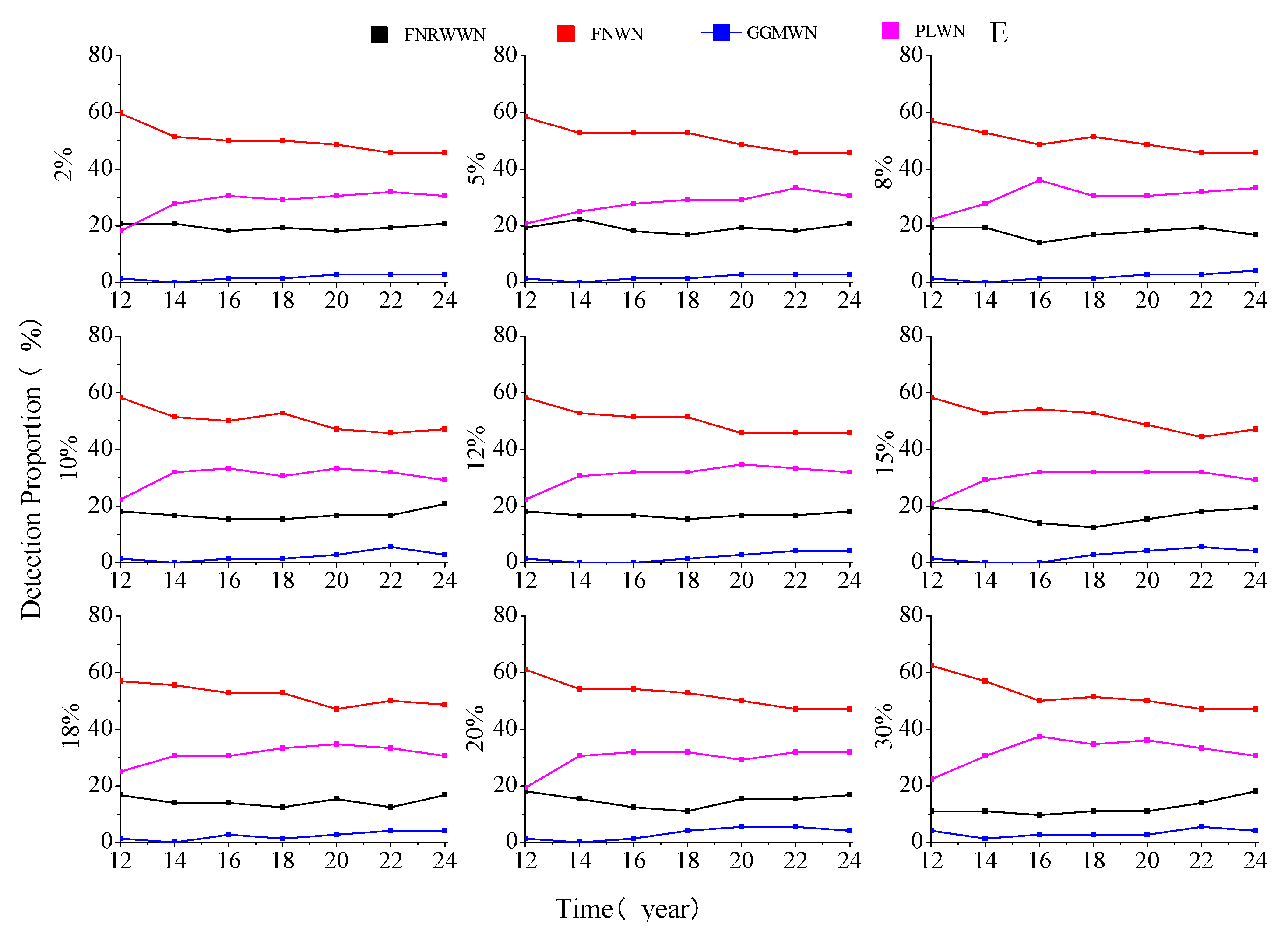
Figure A5.
Evolution of different noise models with various missing rates for the vertical component is shown in Figure A5.
Figure A5.
Evolution of different noise models with various missing rates for the vertical component is shown in Figure A5.
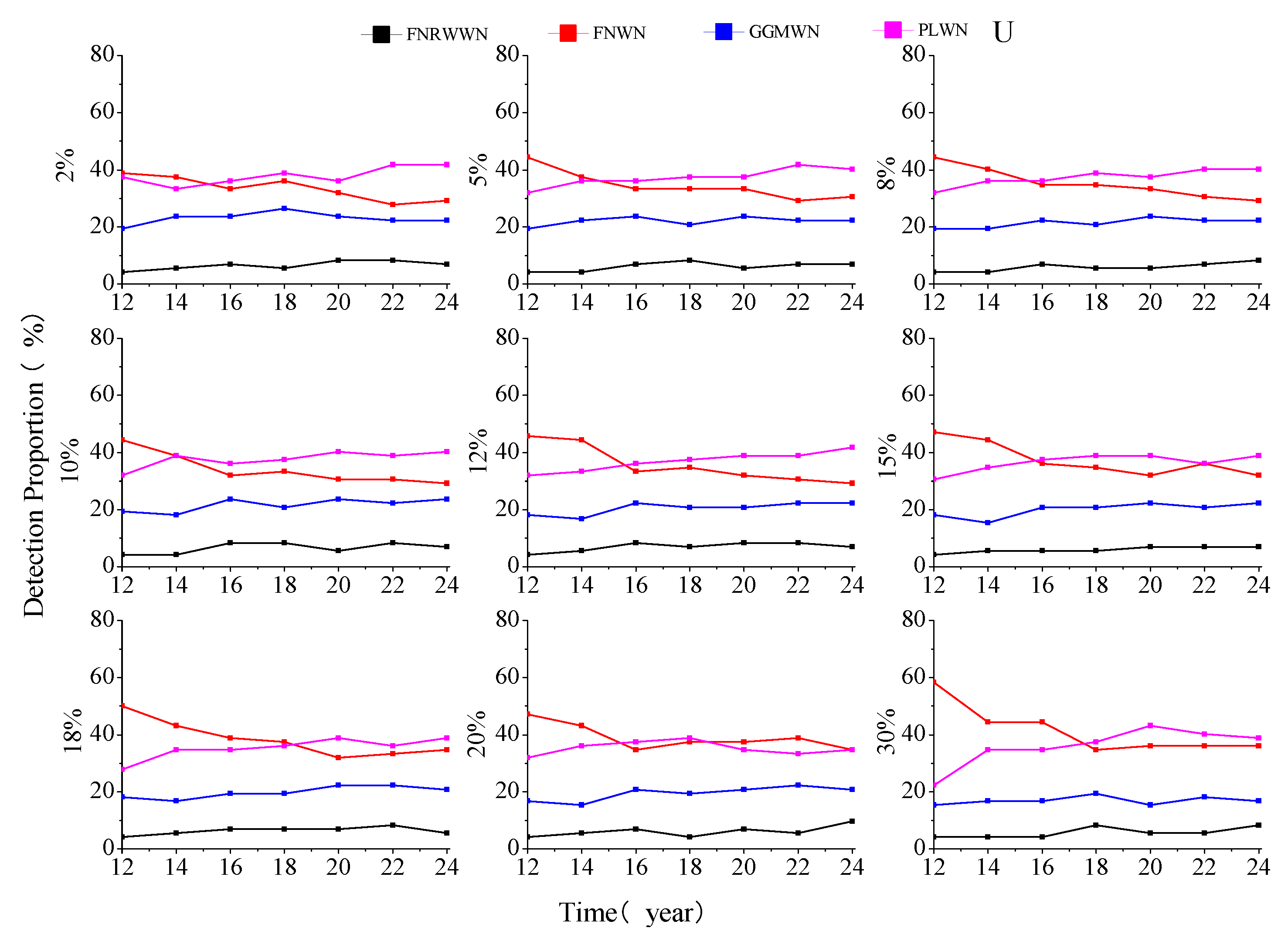
Figure A6.
Evolution of east component velocity law.
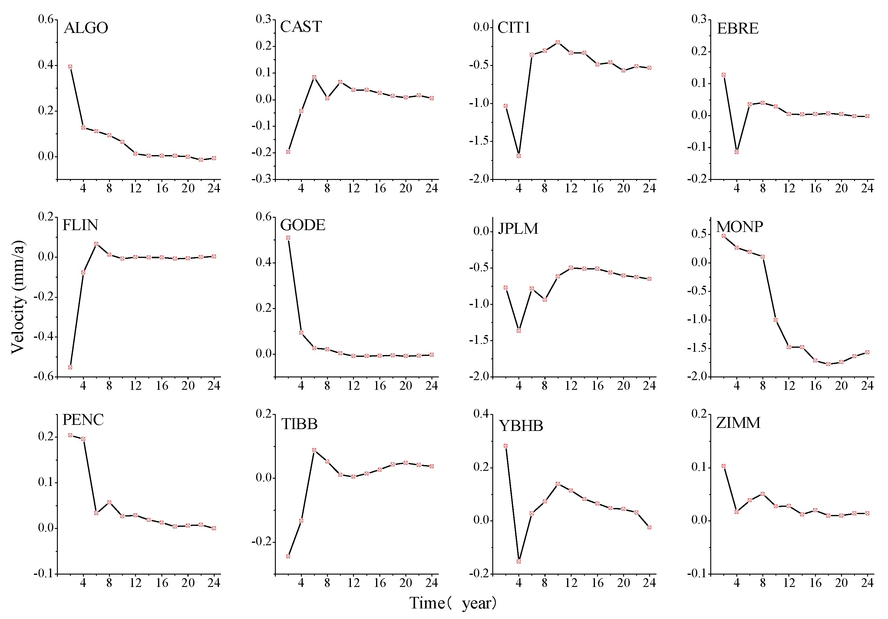
Figure A7.
Evolution of vertical component velocity law.
References
- He, X.; Bos, M.S.; Montillet, J.P.; Fernandes, R.; Melbourne, T.; Jiang, W.; Li, W. Spatial variations of stochastic noise properties in GPS time series. Remote Sens. 2021, 13, 4534. [Google Scholar] [CrossRef]
- Fernandes, R.M.S.; Ambrosius, B.A.C.; Noomen, R.; Bastos, L.; Combrinck, L.; Miranda, J.M.; Spakman, W. Angular velocities of Nubia and Somalia from continuous GPS data: Implications on present-day relative kinematics. Earth Planet. Sci. Lett. 2004, 222, 197–208. [Google Scholar] [CrossRef]
- Fernandes, R.M.S.; Bastos, L.; Miranda, J.M.; Lourenço, N.; Ambrosius, B.A.C.; Noomen, R.; Simons, W. Defining the plate boundaries in the Azores region. J. Volcanol. Geotherm. Res. 2006, 156, 1–9. [Google Scholar] [CrossRef]
- Bock, Y.; Melgar, D. Physical applications of GPS geodesy: A review. Rep. Prog. Phys. 2016, 79, 106801. [Google Scholar] [CrossRef]
- James, T.S.; Morgan, W.J. Horizontal motions due to post-glacial rebound. Geophys. Res. Lett. 1990, 17, 957–960. [Google Scholar] [CrossRef]
- Segall, P.; Davis, J.L. GPS applications for geodynamics and earthquake studies. Annu. Rev. Earth Planet. Sci. 1997, 25, 301–336. [Google Scholar] [CrossRef]
- Troncone, A.; Pugliese, L.; Lamanna, G.; Conte, E. Prediction of rainfall-induced landslide movements in the presence of stabilizing piles. Eng. Geol. 2021, 288, 106143. [Google Scholar] [CrossRef]
- Sheorey, P.R.; Loui, J.P.; Singh, K.B. , et al. Ground subsidence observations and a modified influence function method for complete subsidence prediction. Int. J. Rock. Mech. Min. 2000, 37, 801–818. [Google Scholar] [CrossRef]
- Sauber, J.; Plafker, G.; Molnia, B.F.; Bryant, M.A. Crustal deformation associated with glacial fluctuations in the eastern Chugach Mountains, Alaska. J. Geophys. Res. Solid Earth. 2000, 105, 8055–8077. [Google Scholar] [CrossRef]
- Tregoning, P.; Watson, C.; Ramillien, G.; McQueen, H.; Zhang, J. Detecting hydrologic deformation using GRACE and GPS. Geophys. Res. Lett. 2009, 36. [Google Scholar] [CrossRef]
- Husson, L.; Bodin, T.; Spada, G.; Choblet, G.; Kreemer, C. Bayesian surface reconstruction of geodetic uplift rates: Mapping the global fingerprint of Glacial Isostatic Adjustment. J. Geodyn. 2018, 122, 25–40. [Google Scholar] [CrossRef]
- Turner, R.J.; Reading, A.M.; King, M.A. Separation of tectonic and local components of horizontal GPS station velocities: A case study for glacial isostatic adjustment in East Antarctica. Geophys. J. Int. 2020, 222, 1555–1569. [Google Scholar] [CrossRef]
- Jiang, W.; Li, Z.; van Dam, T. , et al. Comparative analysis of different environmental loading methods and their impacts on the GPS height time series. J. Geodesy. 2013, 87, 687–703. [Google Scholar] [CrossRef]
- He, X.; Montillet, J.P.; Hua, X.; Yu, K.; Jiang, W.; Zhou, F. Noise analysis for environmental loading effect on GPS position time series. Acta Geodynamica et Geomaterialia. 2017, 14, 131–142. [Google Scholar]
- He, X.; Montillet, J.P.; Fernandes, R.; Bos, M.; Yu, K.; Hua, X.; Jiang, W. Review of current GPS methodologies for producing accurate time series and their error sources. J. Geodesy. 2017, 106, 12–29. [Google Scholar] [CrossRef]
- Wang, W.; Zhao, B.; Wang, Q.; Yang, S. Noise analysis of continuous GPS coordinate time series for CMONOC. Adv. Space. Res. 2012, 49, 943–956. [Google Scholar] [CrossRef]
- Bock, Y.; Melgar, D. Physical applications of GPS geodesy: A review. Rep. Prog. Phys. 2016, 79, 106801. [Google Scholar] [CrossRef]
- Mao A, Harrison CGA, Dixon, T.H. Noise in GPS Coordinate Time Series. J. Geophys. Res. Solid Earth. 1999, 104, 2797–2816.
- Hang, J.; Bock, Y.; Johnson, H.; Fang, P.; Williams, S.; Genrich, J.; …; Behr, J. Southern California Permanent GPS Geodetic Array: Error analysis of daily position estimates and site velocities. J. Geophys. Res. Solid Earth. 1997, 102, 18035–18055. [Google Scholar]
- Williams, S.D.; Bock, Y.; Fang, P.; Jamason, P.; Nikolaidis, R.M.; Prawirodirdjo, L. ,... & Johnson, D.J. Error Analysis of Continuous GPS Position Time Series. J. Geophys. Res. Solid Earth. 2004, 109, B03412. [Google Scholar]
- Langbein, J. Noise in GPS Displacement Measurements from Southern California and Southern Ne-vada. J. Ge-ophys. Res. Solid Earth. 2008, 113, 1–12. [Google Scholar]
- Li, Z.; Jiang, W.; Liu, H.; Qu, X. Noise model establishment and analysis of IGS reference station coordinate time series inside China. Acta Geod. Cartogr. Sin. 2012, 41, 496–503. [Google Scholar]
- Agnew, D.C. The time-domain behavior of power-law noises. Geophys Res Letters. 1992, 19, 333–336. [Google Scholar] [CrossRef]
- Mandelbrot, B.B. , & Van Ness, J.W. Fractional Brownian motions, fractional noises and applications. SIAM re-view, 1968, 10, 422–437. [Google Scholar]
- Montillet, J.P.; Bos, M.S. (Eds.) . Geodetic time series analysis in earth sciences. Springer. 2019. [Google Scholar]
- He, X.; Bos, M.S.; Montillet, J.P.; Fernandes, R.M.S. Investigation of the noise properties at low frequencies in long GNSS time series. J. Geodesy. 2019, 93, 1271–1282. [Google Scholar] [CrossRef]
- Bos, M.; Fernandes, R.; Williams, S.; Bastos, L. The noise properties in GPS time series at European stations revisited. EGU General Assembly, Geophysical Research Abstracts. 2013, EGU2013-12825.
- Akaike, H. A new look at the statistical model identification. IEEE transactions on automatic control. 1974, 19, 716–723. [Google Scholar] [CrossRef]
- Schwarz, G. Estimating the dimension of a model. The annals of statistics, 1978, 461-464.
- Bos, M.S.; Fernandes, R.M.S.; Williams, S.D.P.; Bastos, L. Fast Error Analysis of Continuous GNSS Obser-vations with Missing Data. J. Geodesy. 2013, 87, 351–360. [Google Scholar] [CrossRef]
- Amiri-Simkooei, A.R.; Tiberius, C.C.J.M.; Teunissen, P.J.G. Assessment of noise in GPS coordinate time series: methodology and results. J. Geophys. Res. Solid Earth. 2007, 112(B7).
- Amiri-Simkooei, A.R. Non-negative least-squares variance component estimation with application to GPS time series. J. Geodesy. 2016, 90, 451–466. [Google Scholar] [CrossRef]
- Bock, Y.; Nikolaidis, R.M.; de Jonge, P.J.; Bevis, M. Instantaneous geodetic positioning at medium distances with the Global Positioning Systems. J. Geophys. Res. 2000, 105, 28223–28253. [Google Scholar] [CrossRef]
- Bock, Y. ; Moore, A.W. ; Argus, D.;et al. Extended Solid Earth Science ESDR System (ES3): Algorithm Theoretical Basis Document, NASA MEaSUREs project, # NNH17ZDA001N. 2021.
- Bos, M.S.; Fernandes, R.M.S.; Williams, S.D.P.; Bastos, L. Fast error analysis of continuous GPS observations. J. Geodesy. 2008, 82, 157–166. [Google Scholar] [CrossRef]
- Bevis, M.; Bedford, J.; Caccamise, D.J. , II The art and science of trajectory modelling. Geodetic time series analysis in Earth sciences. 2020, 1–27. [Google Scholar]
- He, X.; Hua, X.H.; Lu Tie, D.L.; Yu, K.G.; Xuan, W. Analysis of the Impact of Time Span on GPS time series Noise Model and Velocity Estimation. Journal of National University of Defense Science and Technology. 2017, 6, 12–18. [Google Scholar]
- Montillet, J.P.; Bos, M. Geodetic time series analysis in earth sciences. Springer. Berlin/Heidelberg, Germany, 2019.
- Dmitrieva, K.; Segall, P.; Bradley, A.M. Effects of linear trends on estimation of noise in GNSS position time series. Geophys. J. Int. 2016, ggw391. [Google Scholar] [CrossRef]
- Dong, D.; Fang, P.; Bock, Y.; Cheng, M.K.; Miyazaki, S.I. Anatomy of apparent seasonal variations from GPS-derived site position time series. J. Geophys. Res. Solid Earth. 2002, 107, ETG 9-1–ETG 9-16. [Google Scholar] [CrossRef]
- Peng, Y.; Dong, D.; Chen, W.; Zhang, C. Stable regional reference frame for reclaimed land subsidence study in East China. Remote Sens. 2022, 14, 3984. [Google Scholar] [CrossRef]
- Montillet, J.P.; Melbourne, T.I.; Szeliga, W.M. GPS vertical land motion corrections to sea-level rise estimates in the Pacific Northwest. J. Geophys. Res. 2018, 123, 1196–1212. [Google Scholar] [CrossRef]
- Benoist, C., Collilieux, X., Rebischung, P., Altamimi, Z., Jamet, O., Métivier, L., ... & Bel, L. Accounting for spati-otemporal correlations of GNSS coordinate time series to estimate station velocities. J. Geodyn. 2020; 135, 101693.
- He, Y.; Nie, G.; Wu, S.; Li, H. Analysis and discussion on the optimal noise model of global GNSS long-term coordinate series considering hydrological loading. Remote Sens. 2021, 13, 431. [Google Scholar] [CrossRef]
- Kall, T.; Oja, T.; Kollo, K.; Liibusk, A. The noise properties and velocities from a time series of Estonian per-manent GNSS stations. Geosciences. 2019, 9, 233. [Google Scholar] [CrossRef]
- Kaczmarek, A.; Kontny, B. Identification of the noise model in the time series of GNSS stations coordinates us-ing wavelet analysis. Remote Sens. 2018, 10, 1611. [Google Scholar] [CrossRef]
- Li, W.; Li, Z.; Jiang, W.; Chen, Q.; Zhu, G.; Wang, J. A New Spatial Filtering Algorithm for Noisy and Missing GNSS Position Time Series Using Weighted Expectation Maximization Principal Component Analysis: A Case Study for Regional GNSS Network in Xinjiang Province. Remote Sens. 2022, 14, 1295. [Google Scholar] [CrossRef]
- Wang, L.; Wu, Q.; Wu, F.; He, X. Noise content assessment in GNSS coordinate time series with autoregres-sive and heteroscedastic random errors. Geophys. J. Int. 2022, 231, 856–876. [Google Scholar] [CrossRef]
- Langbein, J. Estimating rate uncertainty with maximum likelihood: differences between power-law and flicker–random-walk models. J. Geodesy. 2012, 86, 775–783. [Google Scholar] [CrossRef]
- Melbourne, T.I.; Webb, F.H. Slow but not quite silent. Science. 2003, 300, 1886–1887. [Google Scholar] [CrossRef]
- Klos, A.; Bogusz, J.; Bos, M.S.; Gruszczynska, M. Modelling the GNSS time series: different approaches to extract seasonal signals. Geodetic time series analysis in earth sciences 2020, 211–237. [Google Scholar]
- Langbein, J.; Svarc, J.L. Evaluation of temporally correlated noise in Global Navigation Satellite System time se-ries: Geodetic monument performance. J. Geophys. Res. Solid Earth. 2019, 124, 925–942. [Google Scholar] [CrossRef]
- Langbein, J. Noise in two-color electronic distance meter measurements revisited. J. Geophys. Res. Solid Earth. 2004, 109. [Google Scholar] [CrossRef]
- Ren, A.K.; Xr, K.; Shao, Z.H. Establishment and analysis of GPS coordinate time series noise model in GEONET. Journal of Navigation and Positioning. 2022, 10, 141–151. [Google Scholar]
Figure 1.
Distribution map of GNSS stations. The red dots represent the location of the GNSS stations used in this study.
Figure 1.
Distribution map of GNSS stations. The red dots represent the location of the GNSS stations used in this study.
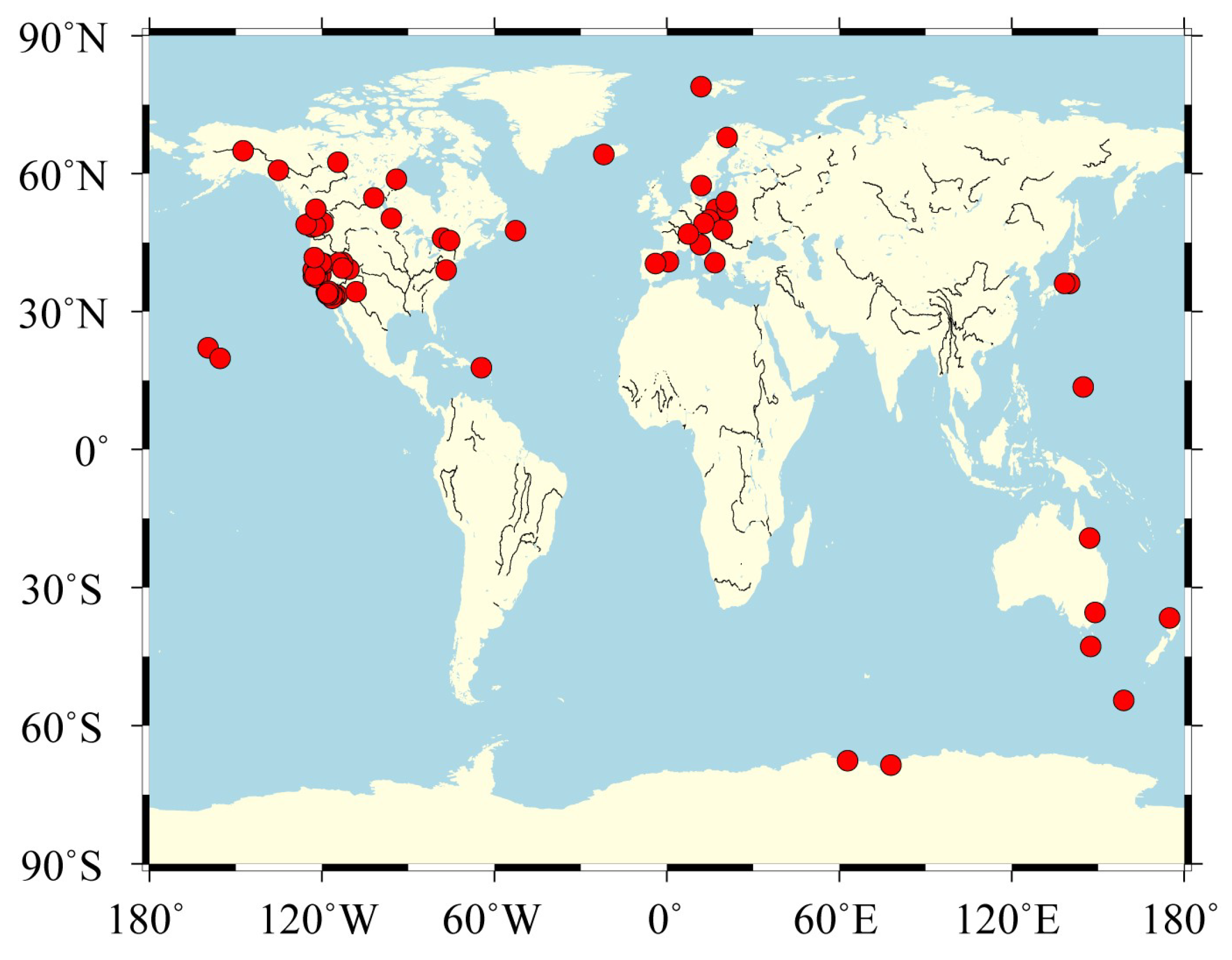
Figure 2.
The 30 year-long simulated time series with different noise models.
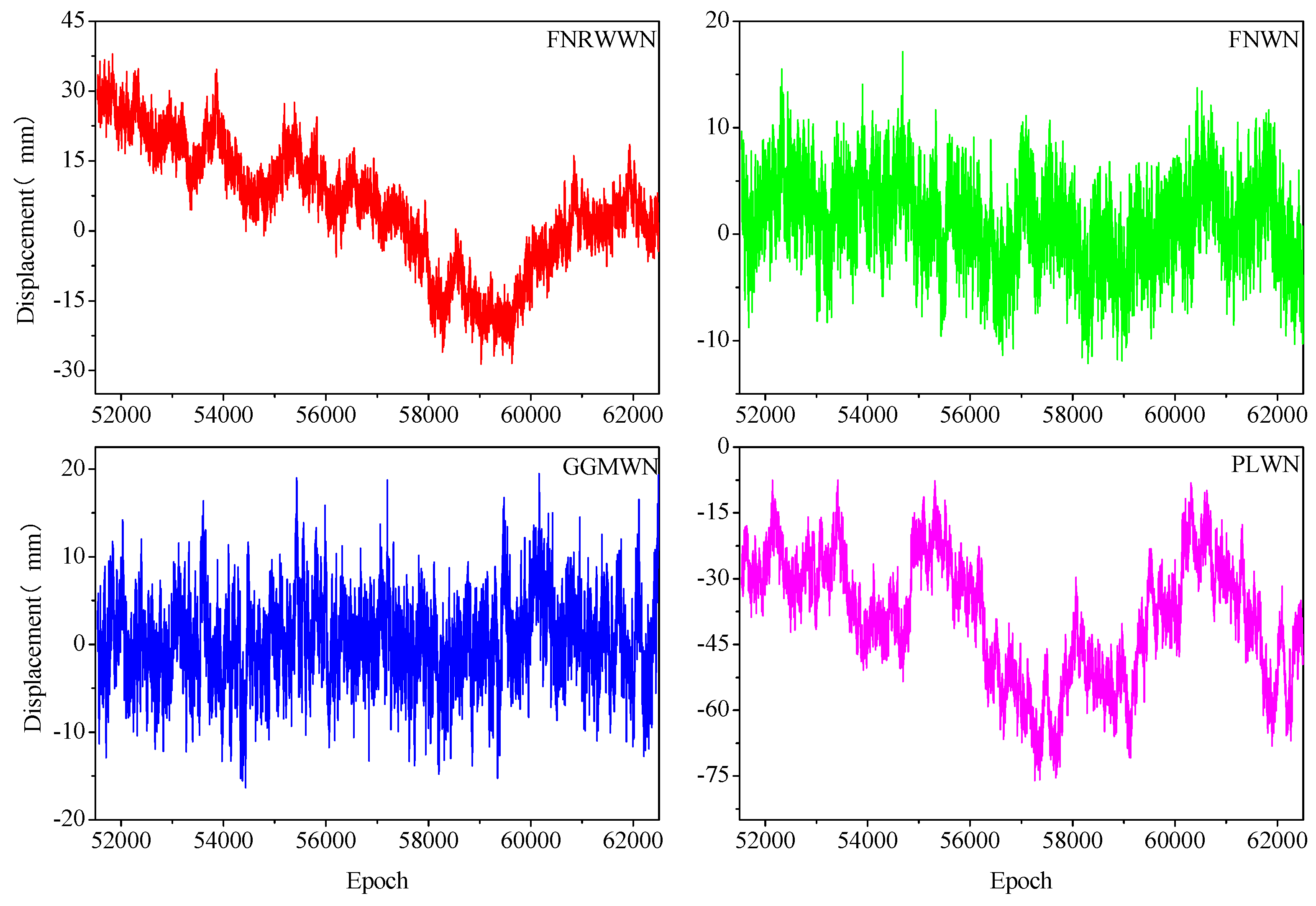
Figure 3.
Probability of detection for different noise models as a function of the missing data (Gap) and length of the time series (Time).
Figure 3.
Probability of detection for different noise models as a function of the missing data (Gap) and length of the time series (Time).
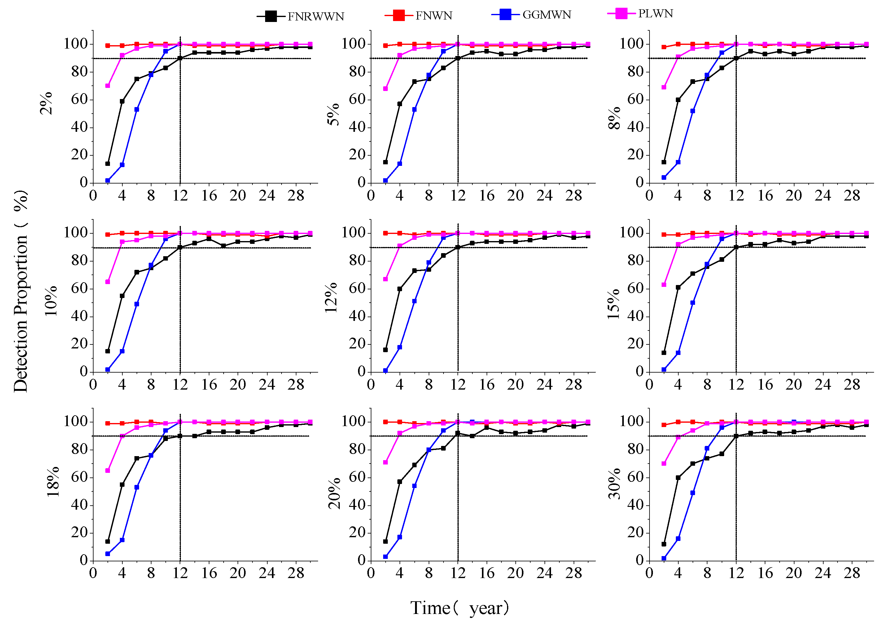
Figure 4.
Spatial Distribution of the noise models for the north component of the GNSS time series for different time period (Green for FNRWWN, red for FNRW, blue for GGMWN, and purple dots for PLWN). The letters (a–i) represent 2a, 6a, 10a, 12a, 16a, 18a, 20a, 22a, and 24a, respectively.
Figure 4.
Spatial Distribution of the noise models for the north component of the GNSS time series for different time period (Green for FNRWWN, red for FNRW, blue for GGMWN, and purple dots for PLWN). The letters (a–i) represent 2a, 6a, 10a, 12a, 16a, 18a, 20a, 22a, and 24a, respectively.
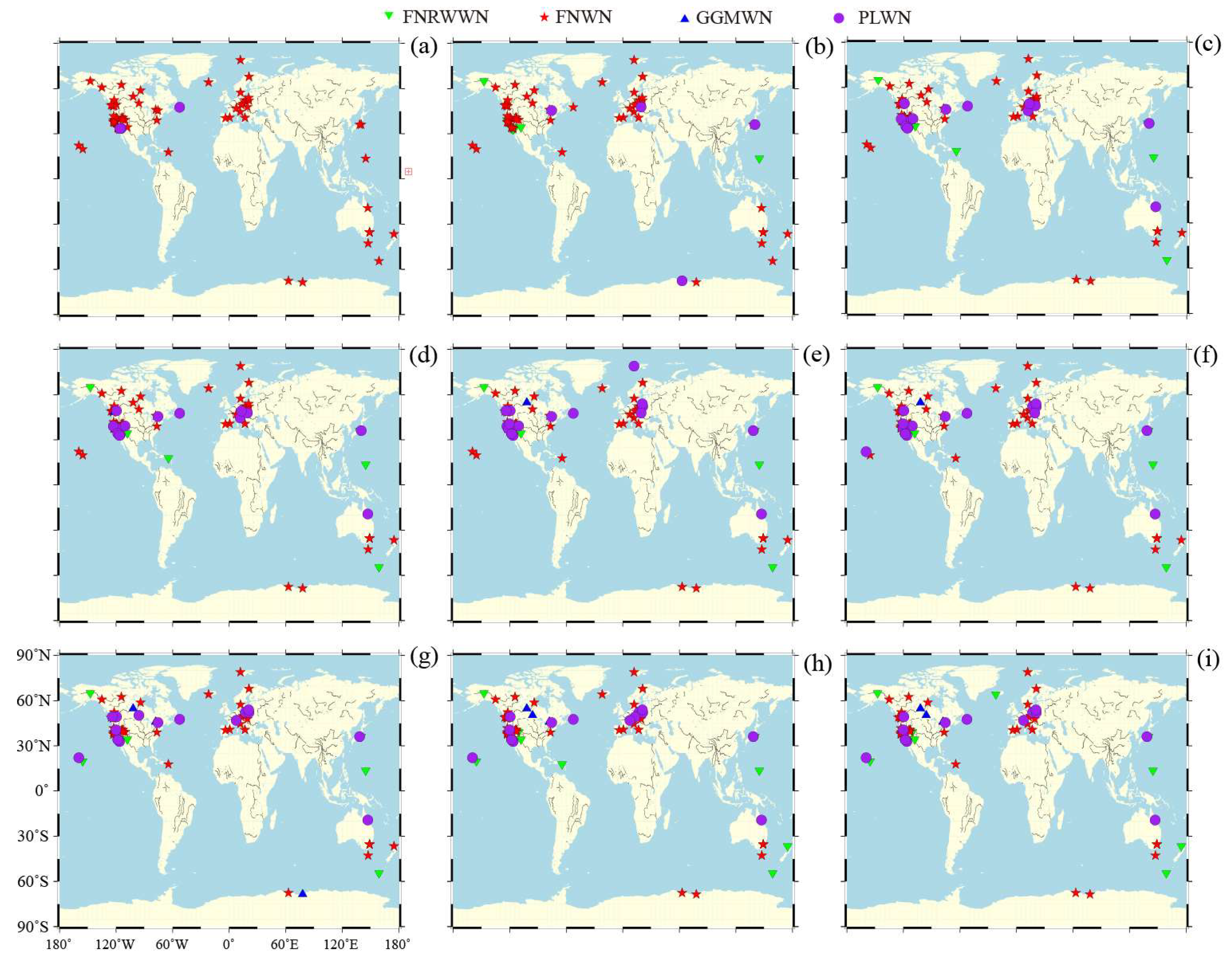
Figure 5.
Variations of the selected noise model using various time series length for 17 stations. (Light blue dots for FNRWWN, blue square for FNWN, yellow triangle for GGMWN, and red diamond for PLWN.).
Figure 5.
Variations of the selected noise model using various time series length for 17 stations. (Light blue dots for FNRWWN, blue square for FNWN, yellow triangle for GGMWN, and red diamond for PLWN.).
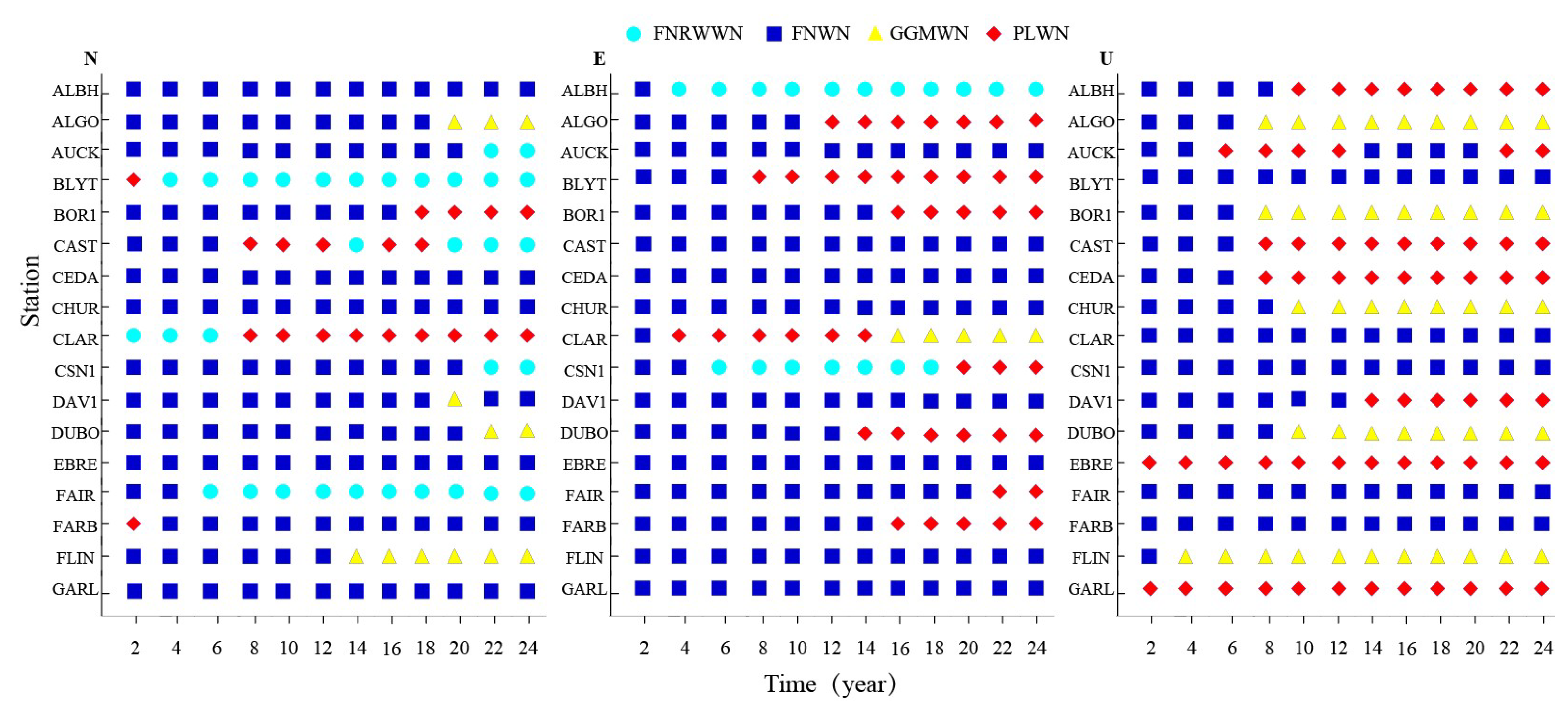
Figure 6.
Evolution of different selected noise models with various missing rates for the north component.
Figure 6.
Evolution of different selected noise models with various missing rates for the north component.
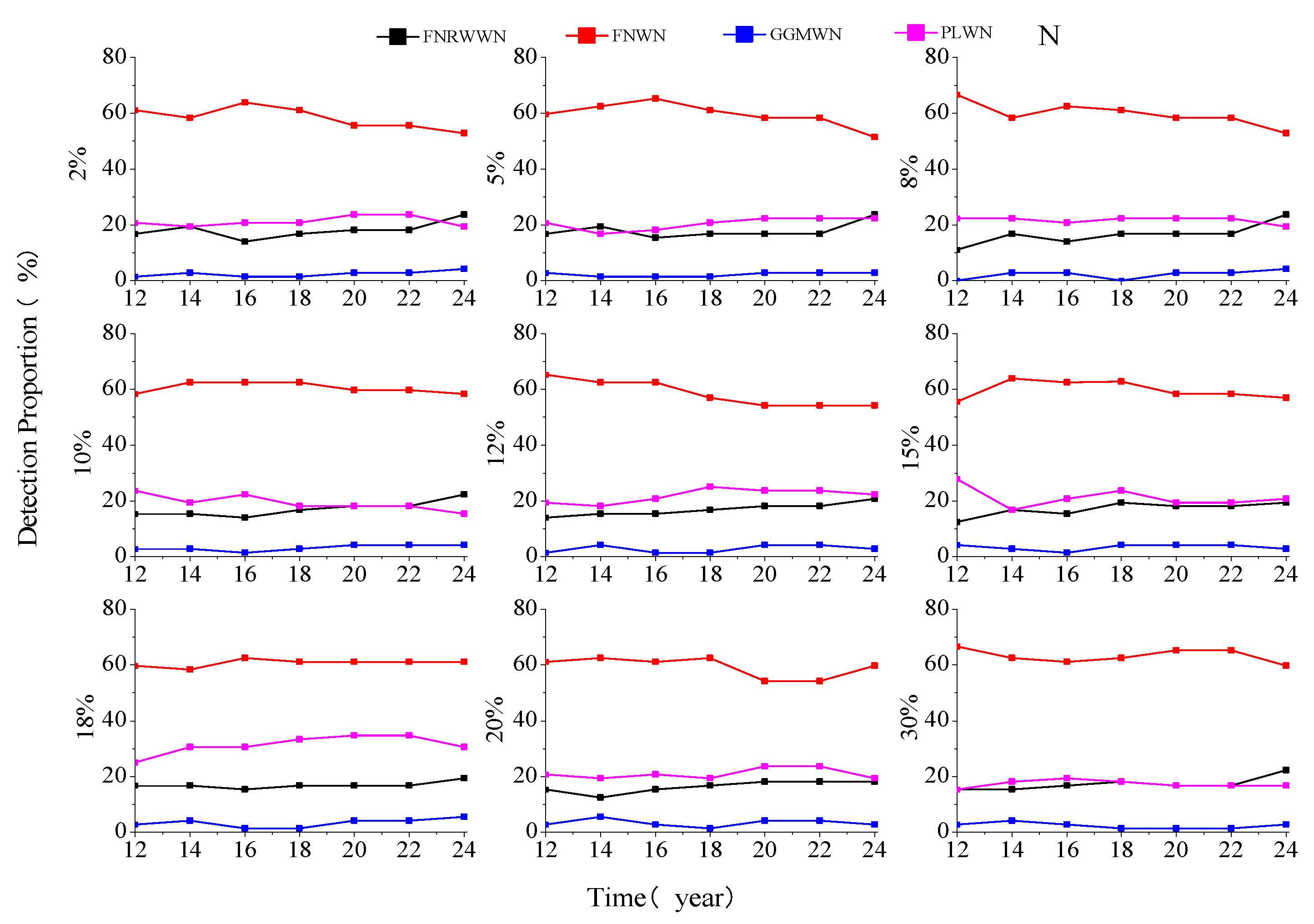
Figure 7.
Mean absolute value changes of simulated time series velocities.
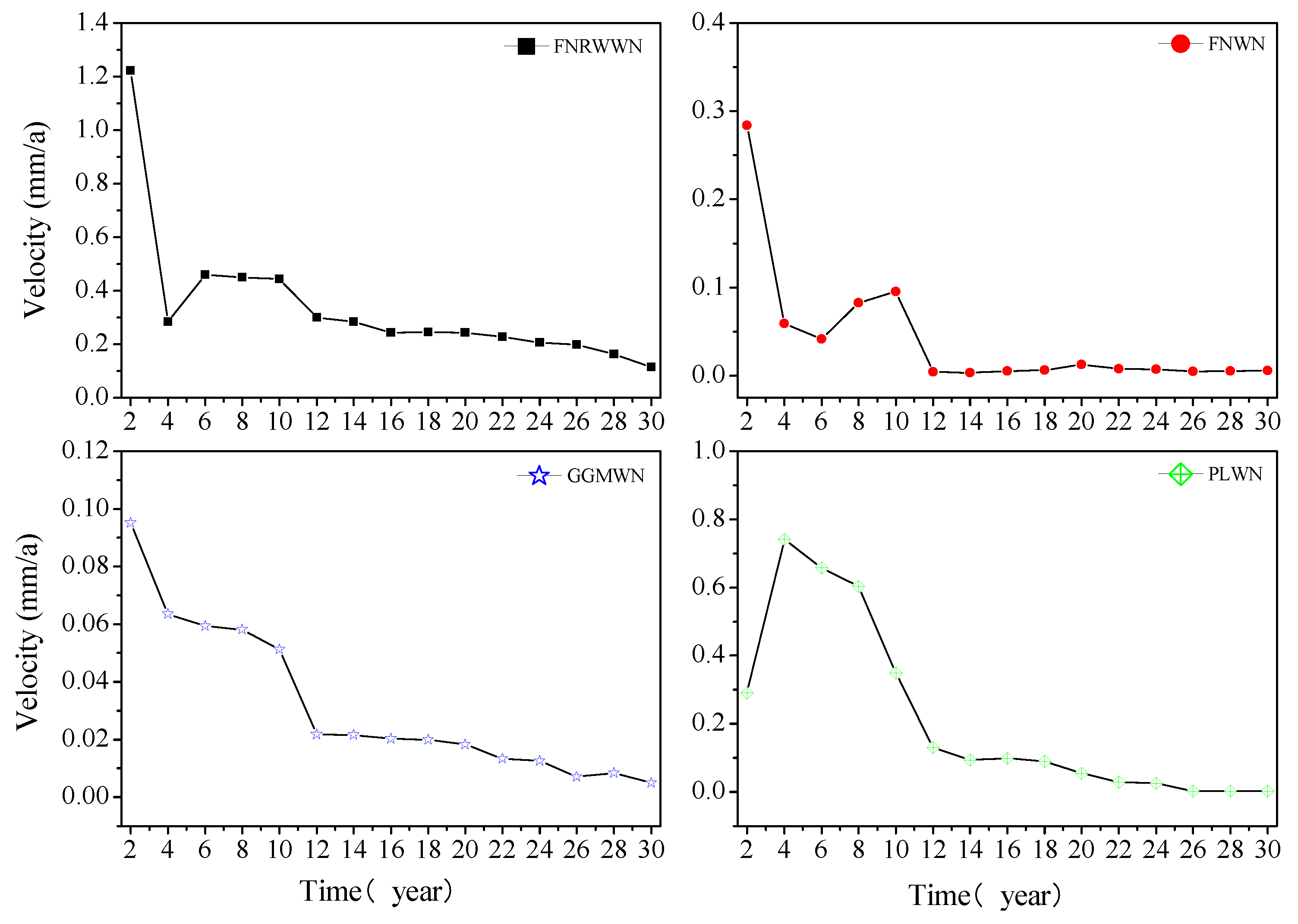
Figure 8.
The variation law of velocity uncertainty of FNWN simulated sequences.
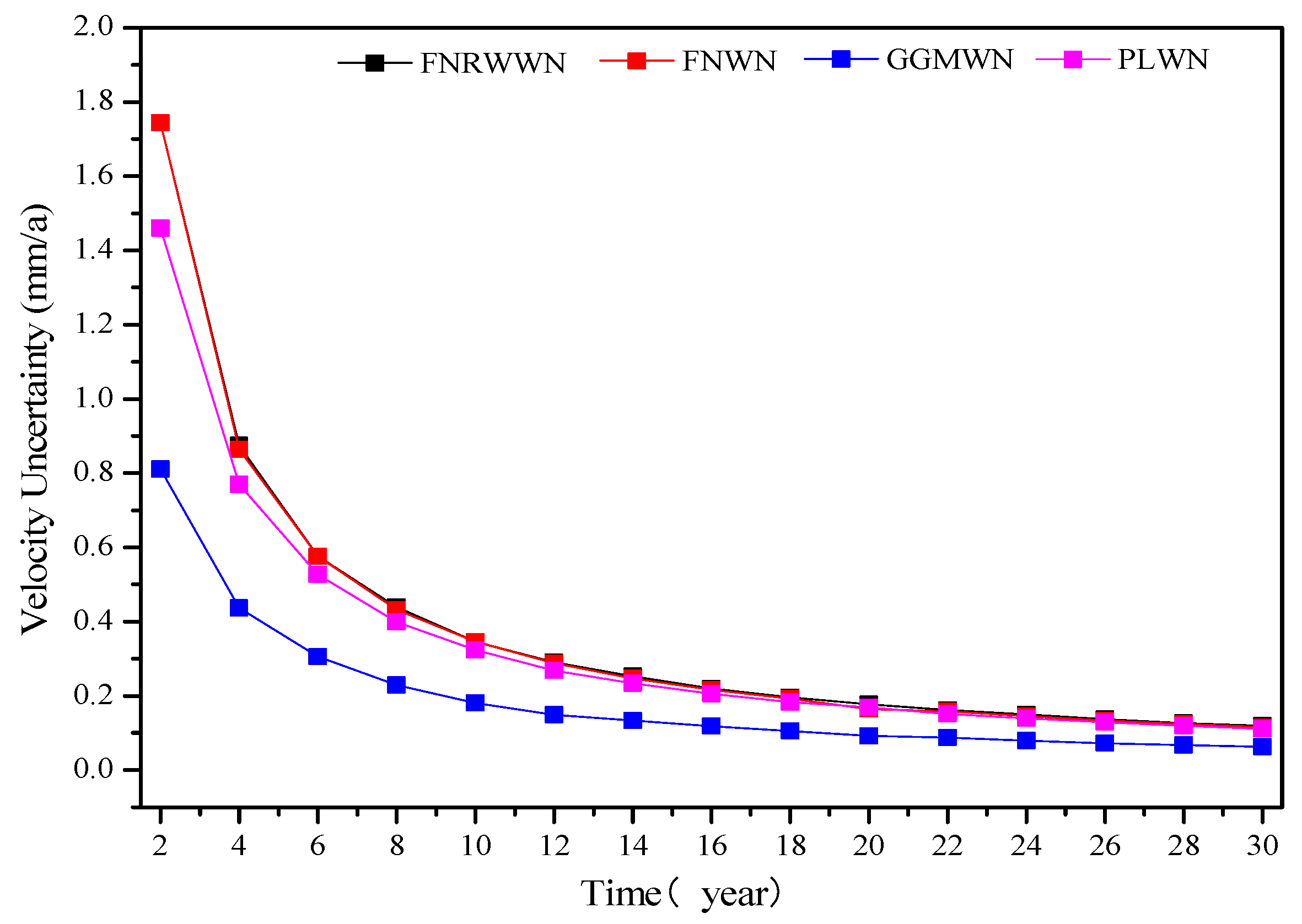
Figure 9.
Mean velocity change curves under different missing rates in simulation.
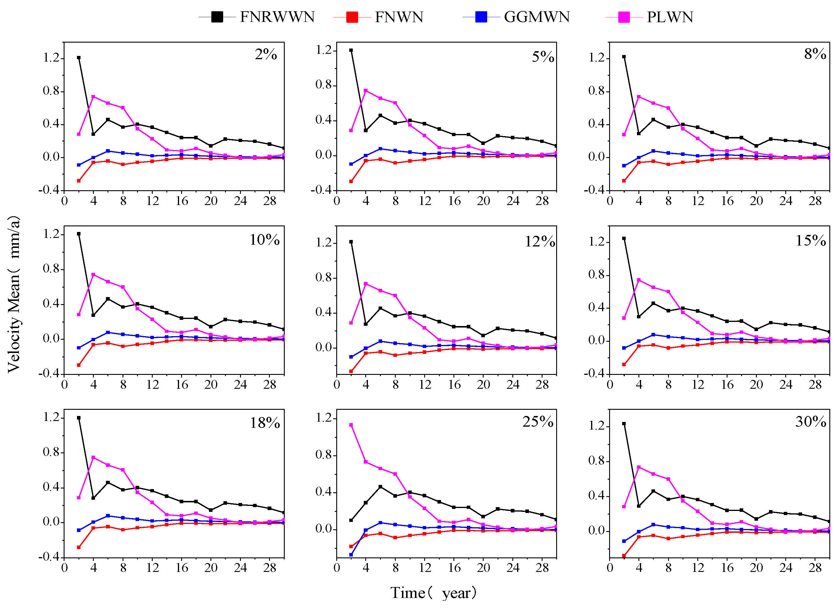
Figure 10.
Distribution curves of velocity uncertainty under different missing rates in the simulated data. (Black square for FNRWWN, red dot for FNWN, green triangle for GGMWN, and blue inverted triangle for PLWN.).
Figure 10.
Distribution curves of velocity uncertainty under different missing rates in the simulated data. (Black square for FNRWWN, red dot for FNWN, green triangle for GGMWN, and blue inverted triangle for PLWN.).
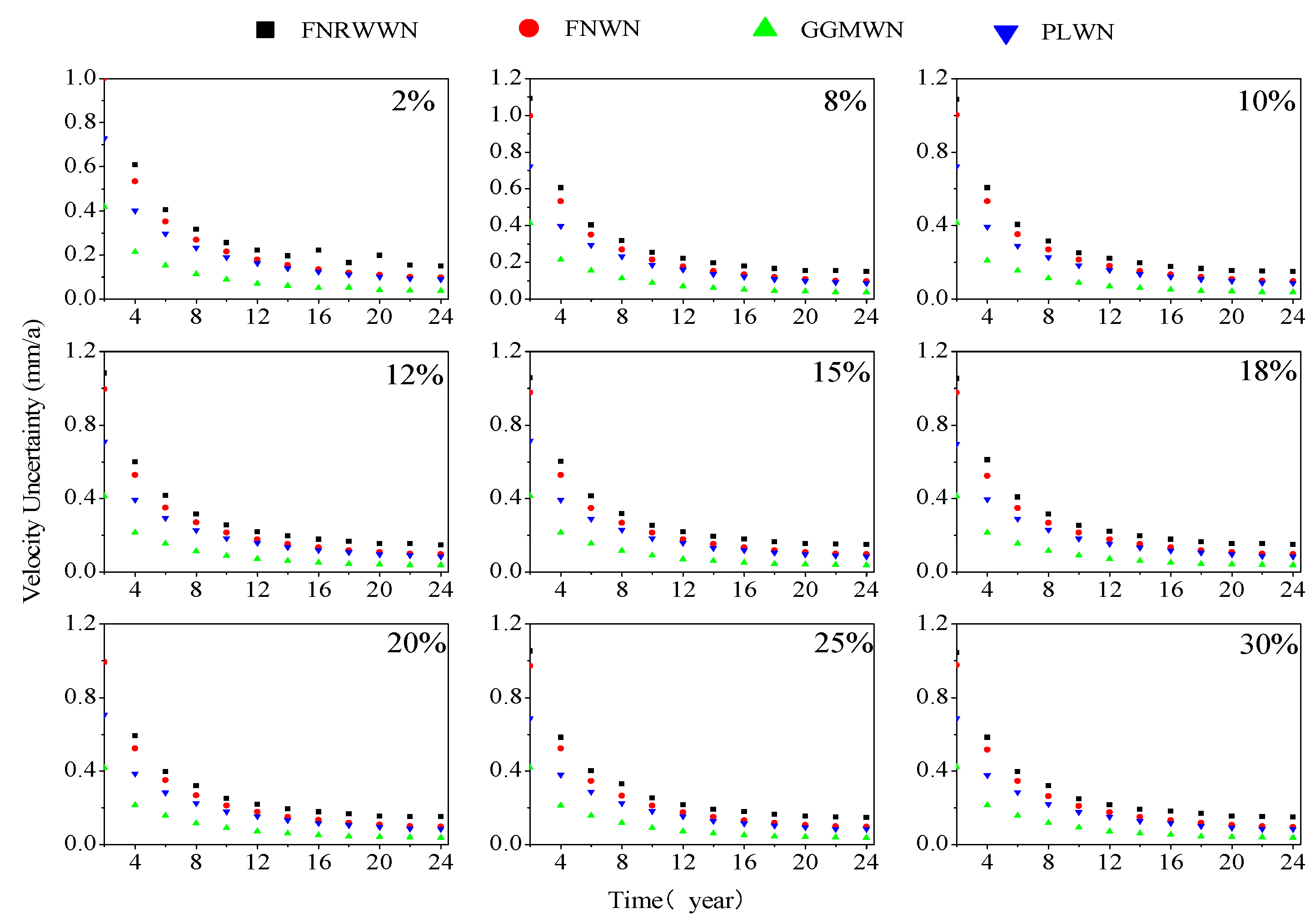
Figure 11.
Evolution of north component velocity law.
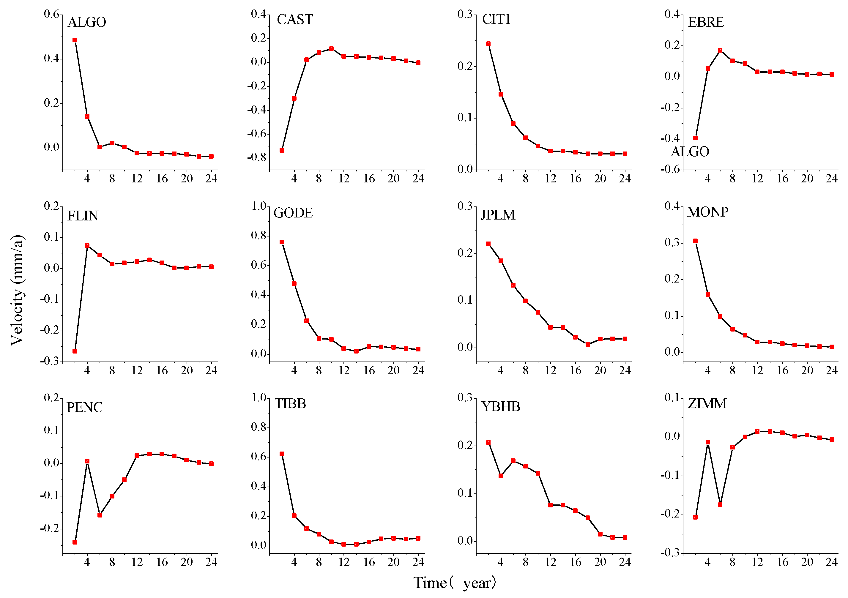
Figure 12.
Curves of velocity uncertainty for different models during different time lengths.
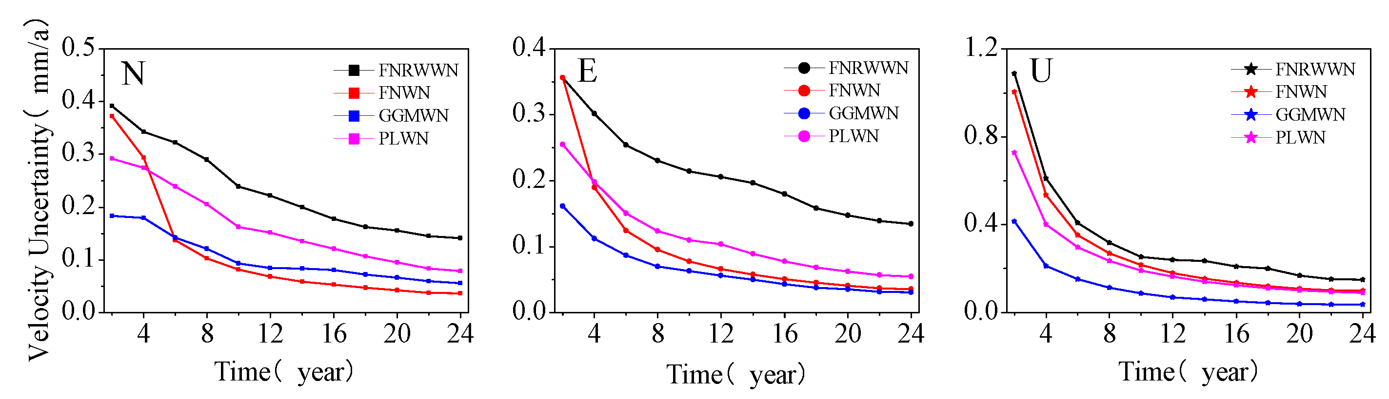
Figure 13.
Evolution of station velocity during different time lengths, in different component station velocities s, and with different missing rates, in the north component, as an example. (Black square for FNRWWN, red dot for FNWN, green triangle for GGMWN and blue inverted triangle for PLWN.).
Figure 13.
Evolution of station velocity during different time lengths, in different component station velocities s, and with different missing rates, in the north component, as an example. (Black square for FNRWWN, red dot for FNWN, green triangle for GGMWN and blue inverted triangle for PLWN.).
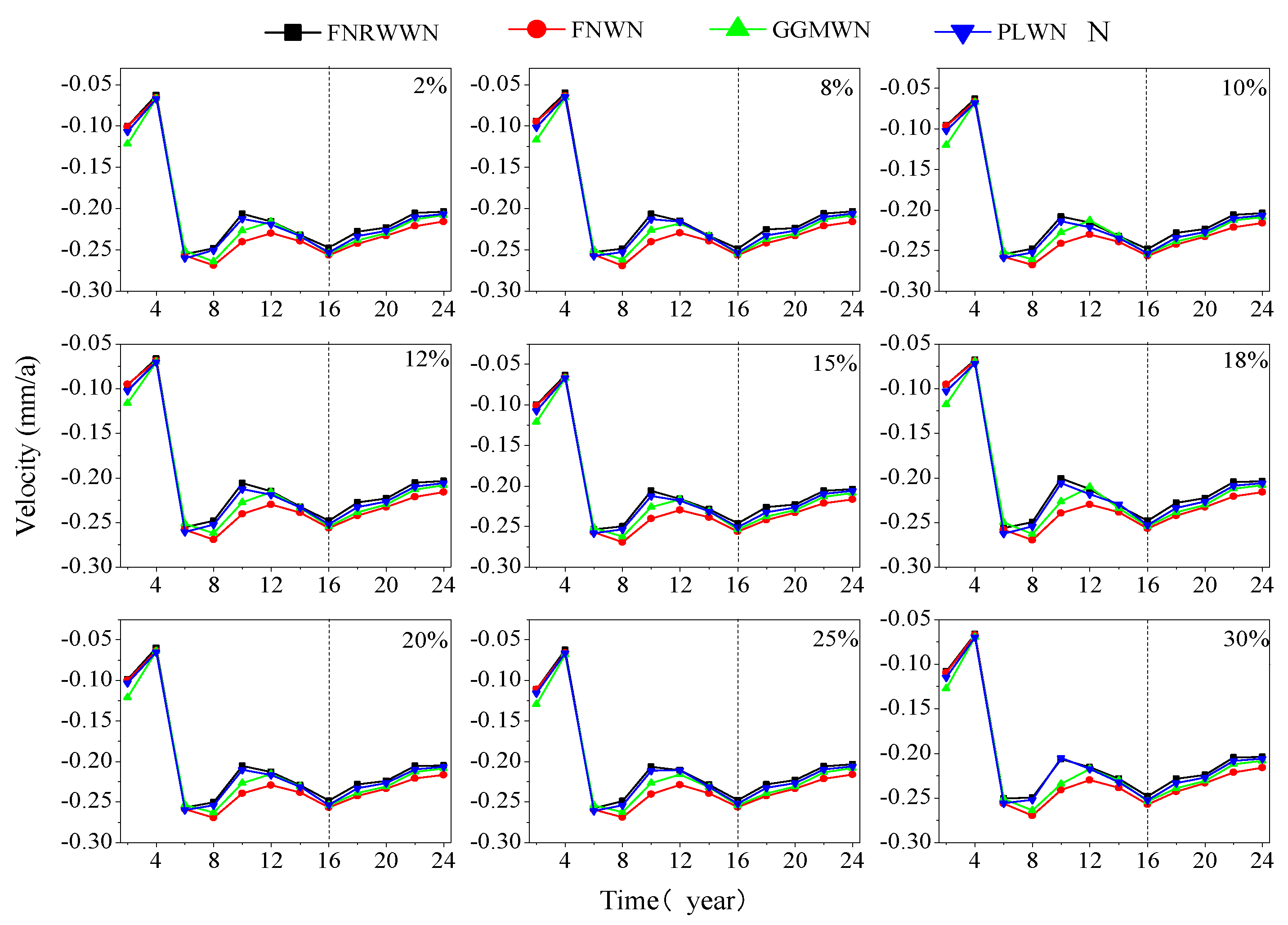
Figure 14.
The distribution of velocity differences in the vertical test with different missing rates in the north component.
Figure 14.
The distribution of velocity differences in the vertical test with different missing rates in the north component.
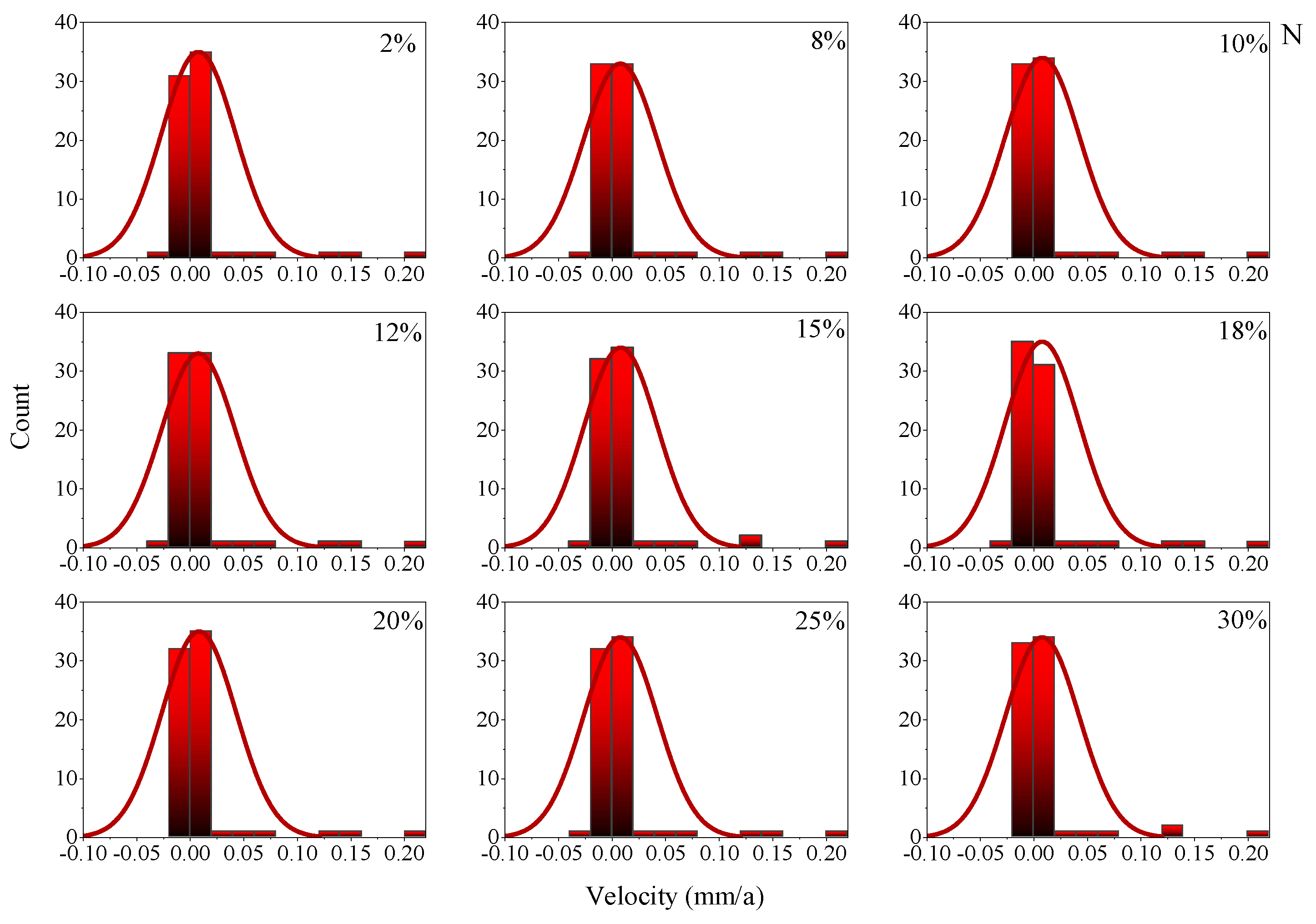
Figure 15.
The distribution curves of velocity uncertainty under different missing rates. (Black square for FNRWWN, red dot for FNWN, green triangle for GGMWN and blue inverted triangle for PLWN.).
Figure 15.
The distribution curves of velocity uncertainty under different missing rates. (Black square for FNRWWN, red dot for FNWN, green triangle for GGMWN and blue inverted triangle for PLWN.).
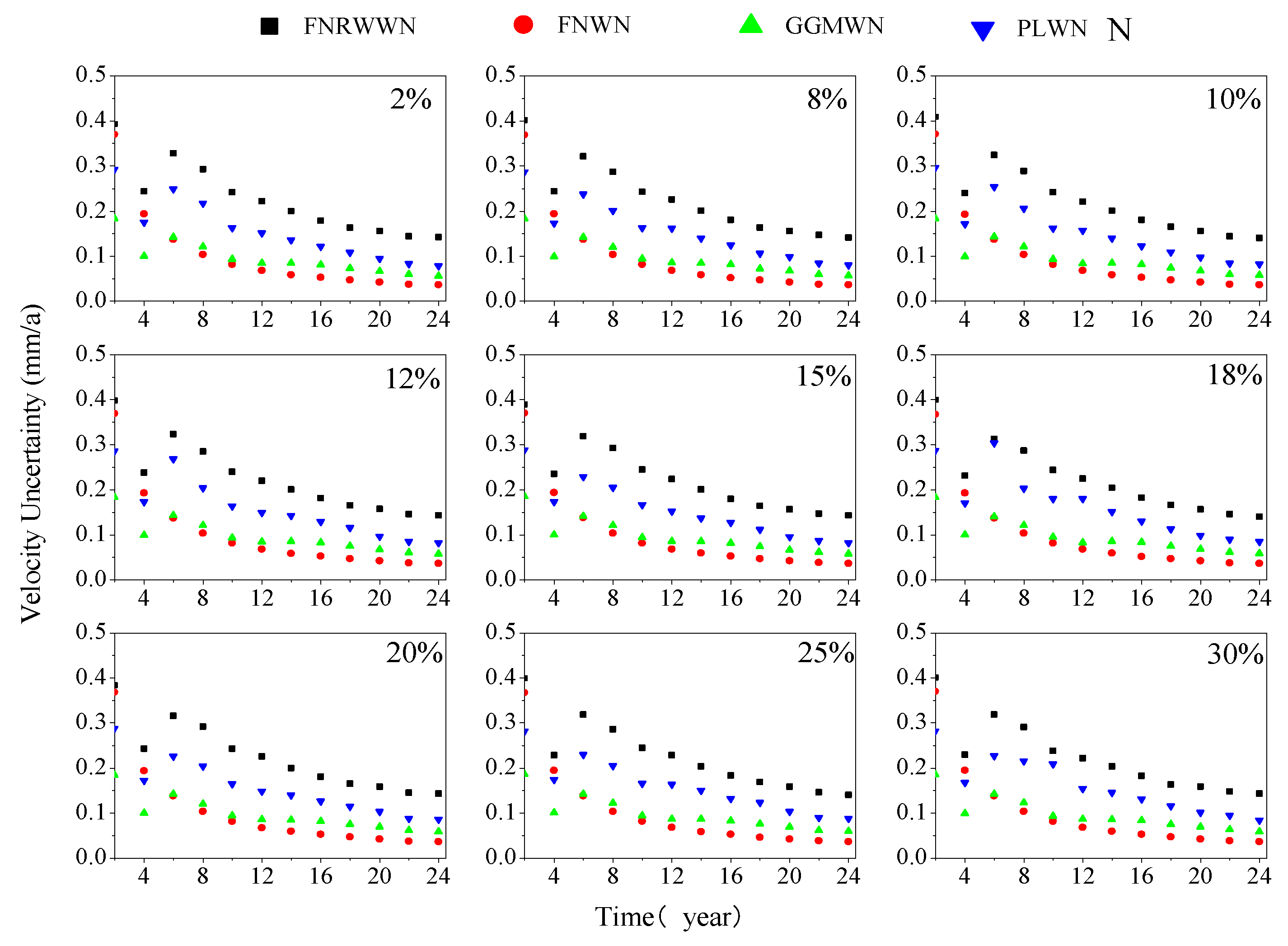

Table 1.
The results of the selected noise model using the BIC_tp and varying the length of the simulated time series.
Table 1.
The results of the selected noise model using the BIC_tp and varying the length of the simulated time series.
| Model | FNRWWN | FNWN | |||||||
|---|---|---|---|---|---|---|---|---|---|
| Length | FNRW WN |
FN WN |
GGM WN |
PL WN |
FNRW WN |
FN WN |
GGM WN |
PL WN |
|
| 2a | 14 | 74 | 0 | 12 | 0 | 99 | 1 | 0 | |
| 4a | 58 | 21 | 0 | 21 | 0 | 100 | 0 | 0 | |
| 6a | 74 | 4 | 0 | 22 | 0 | 100 | 0 | 0 | |
| 8a | 79 | 1 | 0 | 20 | 0 | 100 | 0 | 0 | |
| 10a | 84 | 1 | 0 | 15 | 0 | 100 | 0 | 0 | |
| 12a | 95 | 0 | 0 | 5 | 0 | 100 | 0 | 0 | |
| 14a | 94 | 0 | 0 | 6 | 0 | 99 | 0 | 1 | |
| 16a | 95 | 0 | 0 | 5 | 0 | 99 | 0 | 1 | |
| 18a | 94 | 0 | 0 | 6 | 0 | 99 | 0 | 1 | |
| 20a | 94 | 0 | 0 | 6 | 0 | 100 | 0 | 0 | |
| 22a | 97 | 0 | 0 | 3 | 0 | 99 | 0 | 1 | |
| 24a | 97 | 0 | 0 | 3 | 0 | 99 | 0 | 1 | |
| 26a | 98 | 0 | 0 | 2 | 0 | 100 | 0 | 0 | |
| 28a | 98 | 0 | 0 | 2 | 0 | 100 | 0 | 0 | |
| 30a | 99 | 0 | 0 | 1 | 0 | 100 | 0 | 0 | |
Table 2.
BIC_tp estimation results for GGMWN and PLWN simulation time series.
| Model | GGMWN | PLWN | |||||||
|---|---|---|---|---|---|---|---|---|---|
| Length | FNRW WN |
FN WN |
GGM WN |
PL WN |
FNRW WN |
FN WN |
GGM WN |
PL WN |
|
| 2a | 5 | 0 | 2 | 93 | 29 | 0 | 2 | 69 | |
| 4a | 0 | 0 | 12 | 88 | 7 | 0 | 0 | 93 | |
| 6a | 0 | 0 | 52 | 48 | 3 | 0 | 0 | 97 | |
| 8a | 0 | 0 | 77 | 23 | 1 | 0 | 1 | 98 | |
| 10a | 0 | 0 | 94 | 6 | 0 | 0 | 1 | 99 | |
| 12a | 0 | 0 | 100 | 0 | 0 | 0 | 0 | 100 | |
| 14a | 0 | 0 | 100 | 0 | 0 | 0 | 0 | 100 | |
| 16a | 0 | 0 | 100 | 0 | 0 | 0 | 0 | 100 | |
| 18a | 0 | 0 | 100 | 0 | 0 | 0 | 0 | 100 | |
| 20a | 0 | 0 | 100 | 0 | 0 | 0 | 0 | 100 | |
| 22a | 0 | 0 | 100 | 0 | 0 | 0 | 0 | 100 | |
| 24a | 0 | 0 | 100 | 0 | 0 | 0 | 0 | 100 | |
| 26a | 0 | 0 | 100 | 0 | 0 | 0 | 0 | 100 | |
| 28a | 0 | 0 | 100 | 0 | 0 | 0 | 0 | 100 | |
| 30a | 0 | 0 | 100 | 0 | 0 | 0 | 0 | 100 | |
Table 3.
Comparison of velocity uncertainties of simulation sequences with different background noise models
Table 3.
Comparison of velocity uncertainties of simulation sequences with different background noise models
| Model | Ratio | Model | Ratio | Model | Ratio | Model | Ratio |
|---|---|---|---|---|---|---|---|
| 5.3 | 1.0 | 0.03 | 0.5 | ||||
| 3.5 | 1.9 | 0.5 | 5.2 | ||||
| 2.5 | 1.1 | 0.1 | 2.3 |
Disclaimer/Publisher’s Note: The statements, opinions and data contained in all publications are solely those of the individual author(s) and contributor(s) and not of MDPI and/or the editor(s). MDPI and/or the editor(s) disclaim responsibility for any injury to people or property resulting from any ideas, methods, instructions or products referred to in the content. |
© 2023 by the authors. Licensee MDPI, Basel, Switzerland. This article is an open access article distributed under the terms and conditions of the Creative Commons Attribution (CC BY) license (http://creativecommons.org/licenses/by/4.0/).
Copyright: This open access article is published under a Creative Commons CC BY 4.0 license, which permit the free download, distribution, and reuse, provided that the author and preprint are cited in any reuse.


