Submitted:
17 July 2024
Posted:
18 July 2024
Read the latest preprint version here
Abstract
Drone technology is undoubtedly part of our everyday life these days. The business and industrial use of unmanned aerial vehicles (UAV) can provide favorable solutions in many areas of life, and they are also great for emergency situations and for reaching hard-to-reach places. However, there are many technological and regulatory challenges to overcome in their application. One of the weak links in the operation of UAVs is the limited availability of energy. In order to address this issue authors develop a novel trajectory planning method for UAVs to optimize the energy necessity during flight. For this, an “energy map”, which serves as the basis for trajectory planning, must first be prepared, i.e., the energy consumption of the individual components must be determined. This is followed by configuring the 3D environment including partitioning of the work space (WS), i.e. the definition of free spaces, occupied spaces (obstacles) and semi-occupied/free spaces. On the basis of the partitioned space, the corresponding graph-like path(s) has to be generated, where a graph search-based heuristic trajectory planning can be started, taking into account the most important wind conditions, e.g. velocity and direction. Finally, in order to test the theoretical results, some sample environment will be created, where the proposed path generations will be tested and analyzed. The suggested method is able to find the optimal path in terms of energy consumption.
Keywords:
UAV
; trajectory planning
; trajectory optimization
; 3D environment
; energy map
1. Introduction
The ever-increasing development of drone technology (courier drones, precision agro-culture “agro-drones”, drones used in emergency situations, drones used in different industrial areas, military drones) facing engineers to newer and newer technical challenges [1].
By definition Unmanned Aerial Vehicle (UAV) is an unmanned aircraft (UA) that can fly autonomously, compared with the RPA (Remotely Piloted Aircraft), which is semiautonomous. In addition to these terms, the UAS (Unmanned Aerial Systems) has also need to be define, as a combined aircraft, i.e., the system contains the controller on the ground, the aircraft in the air, and the communication between them, the whole system. The RPA can also be part of a system called RPAS (Remotely Piloted Aircraft System), where the whole system is created from RPA (see above), plus GCS (Ground Control Station) [2].
Basically, there are several classifications of drones. For classic UAVs, this classification can be, for example, the following: multi-rotor, fixed wing, single-rotor, fixed-wing hybrid VTOL (Vertical Take-Off and Landing), MAV (Micro Air Vehicle: < 1[g]), sUAS (small UAS:< 25[kg]), …etc., but what is more important from the research point of view, that the drone belongs into “open (public) category”, or “specific-category” (drones (UAVs) over 25kg). There is also the “game category” (drones under 120-gram weight), which is irrelevant for this study.
In this project the first two categories can be considered, because of their flight altitude, 120 [m] over the nearest point of ground, for “public category” drones. This dimension will be important in 3D map creation of the flying-environment of the drone.
1.1. Brief Description of the Aims
One of the weak links in the operation of drones is limited energy availability. This idea formed the basis for the development of the proposed trajectory planning method, which uses the energy as effective as possible (optimally) during the flight. This required, first creating an "energy map" of a drone, where the components have to be determined which consume the most energy, and the trajectory planning mechanism has to be adjusted accordingly. Secondly, the weather reports, especially wind reports of the terrain, must be available during the path planning of the drone.
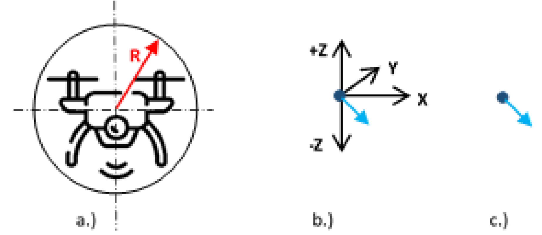
The energy map creation must be followed by the 3D environment configuration. Through this process the drone understands the environment. As a result of the partitioning of the “work space” (WS), the following areas are created: “free spaces”; “occupied areas” and “semi -occupied/-free spaces”. The occupied areas contain the obstacles, while semi-occupied are partly contains them. Certainly based on specified resolution of partitioning the semi-occupied areas can be further partitioned, depending on the used partitioning method. Once the environment has been partitioned, the modelling can begin. By the modelling the point represented drone can move on configured WS. Configured obstacles are those, whose dimensions are increased by the radius (R) of the sphere drawn around the drone (see Fig.1). In this way the physical dimensions of the drone are considered in the WS model. Of course, extra “safety zones” can be added based on requirements of the user.
Figure 1.
The process of the creation of point representation. (a) The drone and the sphere around the drone by “R” radius; (b) The point represented drone by its coordinates and orientation; (c) The point represented drone by its orientation (this will figure in environment model).
Figure 1.
The process of the creation of point representation. (a) The drone and the sphere around the drone by “R” radius; (b) The point represented drone by its coordinates and orientation; (c) The point represented drone by its orientation (this will figure in environment model).
1.2. State–of-the-Arts
The surveyed “state-of-the-arts” can basically be divided into 3 groups.
The focus of these publications is the evaluation of the energy consumed by the different parts of the drone, based on which energy weights can be assigned to the different parts of the path. From the created “energy map” of the drones it is clear that most of the energy is consumed by the drive rotors. The power of these rotors is highly dependent on velocity, ascending, descending and the air resistance of the drone. The velocity can be controlled by the ESC (Electronic Speed Controller) or FC (Flight Controller).
These publications serve a good basis for design a novel space partitioning and path planning algorithm. A shortcoming of the surveyed documentations is that almost none of them deal with partitioning of the WS. There are two possible reasons for this as follows: a.) Drones are equipped with the environmental sensing equipment (RADAR or LIDAR sensors, cameras, vision systems, US sensors, etc.). b.) Drones flying a visible distance and are controlled via some joystick or remote controllers. GPS is a standard equipment of drones.
Among the examined publications, there is no one that deals with the topic of energy used in aviation. In order to take this condition into account, it is inevitable to establish several routes between the START and GOAL positions, review these paths and select the one that requires the least energy for execution. Unfortunately, this will work in static environment, because recalculating and re-weighting the path-segments takes some time, depending on the complexity of the flight control (FC) processor.
- Last but not least, some legal information about drone flight and civil aviation can be found that should be considered during the study (see [21]).
Drone flight rules (policies) in the EU, but indeed the world, have not yet been fully developed. There are some local provisions, but they are not completed. There are some drone categories (A, B, C), some flight altitudes, and the required permissions for drone flights (drone driving licenses). In this study, is the most significant of these regulations is to keep the 120[m] altitude from the nearest ground point.
2. Preliminary Studies
In this section the studies about the drone energy consumption and the work space partitioning will be discussed.
2.1. Studies About the Drone Energy Consumption
There are different types of drones regarding power supply.
Figure 2.
Classification of the drones regarding power supply (the energy supply of the actual drone used in the article is highlighted).
Figure 2.
Classification of the drones regarding power supply (the energy supply of the actual drone used in the article is highlighted).
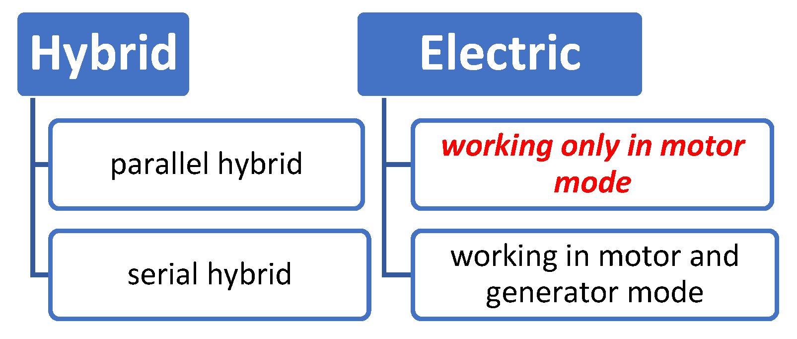
In case of hybrid systems, some EMS (Energy Management Strategy) system usually regulates and controls the efficient energy consumption. These EMSs can be based on different strategies, such as: Rule based systems; Intelligent based systems (Fuzzy or NN); Optimization based; …etc. Classic electric UAVs, which operate only in motorized mode (where there is no recharging of battery) lack these systems, and energy savings has to be ensured by another approach. This is why energy-efficient path planning was developed in this project.
The energy consumption of the drone can be defined in two ways:
- practically: by direct measuring of the amps consumed by different parts of the drone.
- theoretically: with calculations of the energy consumptions of the parts.
For energy consuming calculations the following relations has to be considered as a minimum. Engine power can be calculated based on forces, torques and moments about x/y axis. Generally, the Newton’s Laws are used to calculate forces and moments. See Figure 3 for a better understanding of the equations.
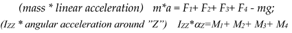
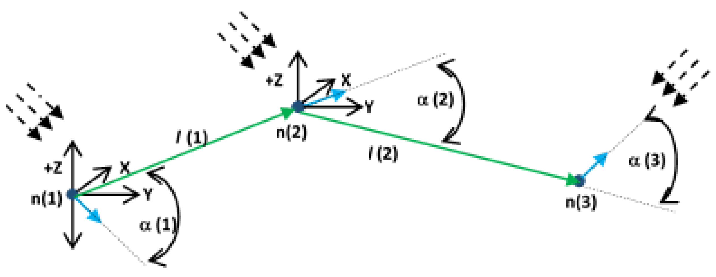
In general, the flight lift forces (F1 – F4) and MX, My moments, can be calculated as follows:
where “L” is the distance between 2 rotors.
The operation’s conditions can be stated by the following relations:
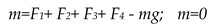
- Hovering motion: Equilibrium conditions for hovering: mg=F1+ F2+ F3+ F4; and all moments = 0;
Equation of motion:
- 2.
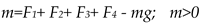
- Rise/fall motion: Conditions for operations: mg < F1+ F2+ F3+ F4 = rise; mg > F1+ F2+ F3+ F4 = fall; and all moments = 0;
Equation of motion:
- 3.
- Yaw motion: conditions for hovering mg = F1+ F2+ F3+ F4 ; and all moments ≠ 0;
Equation of motion:
- 4.
- Pitch / Roll motion: conditions for hovering mg < F1+ F2+ F3+ F4 ; moments ≠ 0;
Equation of motion:
For exact description of the forces and exact modelling of the drone, it is unavoidable to know the rigid-body dynamical relations in 3D environment. Initially, the reference coordinate system has to be set up, as well as related movements. Afterward, the effects on the drone has to be considered, as follows:
- aerodynamic forces: friction and drag of propellers rotating in air
- secondary aerodynamic effects: blade flapping, ground effect, local flow fields
- inertial counter torques: gravitation, acting at the center, affect the rotation of propellers.
- gyroscopic effect: change in the orientation of drone body and plane rotation of propellers
Then the dynamic equation can be written as follows:
where: v – linear velocity (this is the origin linear velocity of the drone, what will be modified by the wing velocity, see eq. (17) vresulting), ω - angular velocity, α - angular acceleration, I - moment of inertia, a - linear acceleration, m - mass, F - total force, τ - total torque. To be clear, about the technical terms, used previously, and understand the energy consumptions, look Figure 4.
3. The Energy Evaluation
Many ideas and calculations (see equations (9)-(12)) have been applied, -maybe with a slightly different interpretation-, to the energy calculations from [23]. In a very general way, the energy consumption of the drone can be summarized as follows:
where, E(anything)= P(anything)*t
Etotal= Eprocessors+ Emotors + Ecommunication + Eperipherials
Let assume some constant and very low energy for (Ecommunication + Eperipherials). The energy consumed by processor(s), can be specified depending on control system complexity:
Furthermore, the energy consumed by motors:
where the dominant energy is:
Emotors= Etakeoff(a,w)+ Ehover(a,w,t)+ Emove(w,s,t,ρ)
Emove(w,s,t,ρ)= Edrag(d,ρ,kdrag,Seff)+ Ekinetic(w,s)
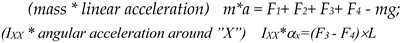
This Emove(w,s,t,ρ) is dominant and important, regarding different air conditions (this will be modelled later in space model). After calculations for a particular case the following “average energy map” of the drone can be created, see diagram below (Phantom 4 drone pro/pro+ series).
Figure 5.
The generalized energy consumption of drone.
4. Environment Description and Work Space Partitioning
Most of the drones are equipped with modern positioning and distance-measuring sensors. The minimum requirements and the most modestly equipped drones contains GPS and a few range measuring LEDs for obstacle detecting. Standard drones usually include the following positioning sensors: GPS, front/rear LEDs, camera system, forward/downward/rear vision systems, infrared sensing system, barometer, etc. Drones with basic equipment, based on FC complexity, can be controlled in different flight modes.
- P-mode (positioning): works best when the GPS signal is strong. In addition to GPS, other sensors are used: stereo vision system, infra sensing system – obstacle avoiding, moving target tracking;
- S-mode (sport): maximum maneuverability. Obstacle sensing disabled.
- A-mode (altitude): only uses the barometer to sense altitude. Positioning is no longer available.
Regarding the work space partitioning, the current drone flight rules must be kept. The most important:
- keep the altitude of 120 [m]
- keep at least 30[m] away from other people
- keep the drone in line-of-sight
From the above, from this study point of view, the first one is the most important, because it limits the volume (space) to be partitioned. On the other hand, if the drone is kept in visual line-of-sight (LoS), the WS partitioning may seem redundant, but the drone will not always be in LoS. The configuration of the WS can always be useful in the operation of unmanned aircraft, because in many cases, if one of the sensors is not working properly, the FC can only rely on the predefined path on the WS model.
There are lot of 3D partitioning methods, such as 4-tree (2D partitioning), 8-tree (3D partitioning, split around a point), KD-tree (partitioning along one dimension), R-tree, and the most general is the Grid (cube) rasterization.
The basic concept of 4/8-tree partitioning: the area/space is divided into 4/8 subparts. Another division is made only on those squares/cubes, where the obstacles are, or part of obstacles can be found. As a result, the resolution of the division increases, as we are get closer to the obstacle.
A KD-Tree is a binary tree in which each node represents a K-dimensional point (hyperspace).
R(rectangle)-Tree groups nearby objects and represents them with their minimum bounding rectangle at the next higher level of the tree [15].
Voxel grid partitioning is the simplest, popular, but not really effective, because the dimensions of the blocks (cubes) remain the same, regardless of the proximity of the obstacle. On the other hand, the calculations are simple, that is why this partitioning is used in the model studied in this paper.
5. Creating the Polygonal Graph over the Work Space
After the successful division of the work space it is easy to create the “Occupancy Map” of the space, where the empty cubes represent the “Free Spaces” (FS).Based in this map the obstacle-free route planning is available. A simple model of the above mentioned method is represented on Figure 6, where the drone will fly between the residential building.
The “graph-like”, i.e., topological map of free environment is created by the connecting the center-points of the neighbouring blocks in such a way that the connecting line cannot touch the occupied spaces (blocks marked in blue dots).
On Figure 5, a scaled 15x15x15 units WS represented and partitioned by cube grid, where the Center Points of the cubes are calculated and the occupied cubes are coloured blue. SW support is ensured by Python package, where the different tools are activated and suited for the requirements. Moreover, the Center Points represent the nodes, while the connecting lines are the edges of the graph. If the neighbouring center points are connected, resulting in 22 lines, 6 of which are the lateral adjacencies (shorter lines) and the rest are diagonal adjacencies (longer lines). The mathematical formula for length calculations is simply based on Pythagorean axiom: , where the indices <i, j> are the number of nodes resp. edges.
5.1. The Weighting Mechanism of the Graph, Calculations of the Weights of Nodes and Edges
Let the graph “G” be defined as follows: G=〈n,e〉, where n(i) – are the nodes of the graph, and e(j) - are the edges of the graph. The weighting of the graph is divided into two phases. In phase 1, the edges are weighted related to the length (l(j)) of the edge e(j), then, in phase 2 the energy demand of the node (E(i)) is calculated using the previously defined mathematical expressions.
5.1.1. The Energy Demand Calculation of the Node
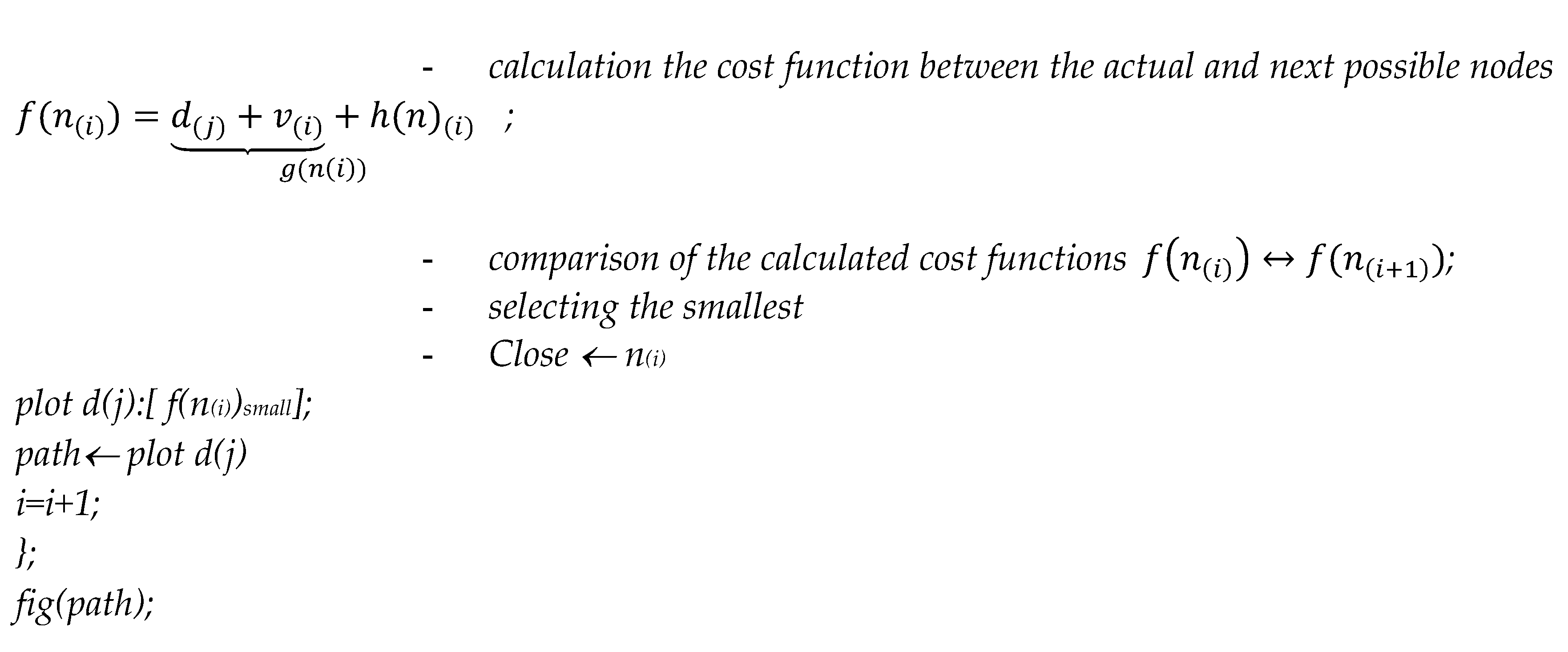
To evaluation the energy demand of the node, the following conditions has to be considered: the orientation of the drone (see: yaw/pitch/roll –equations of motion (6), (7)) [24]; altitude changing (see: rise/fall –equations of motion (5)); air resistance and wind directions (see: Emove – calculation, eq.: (11)). But basically in Emotors eq.: (10), all these calculations can be find. Consequently, the final energy demand of graph-node (i) can be calculated:
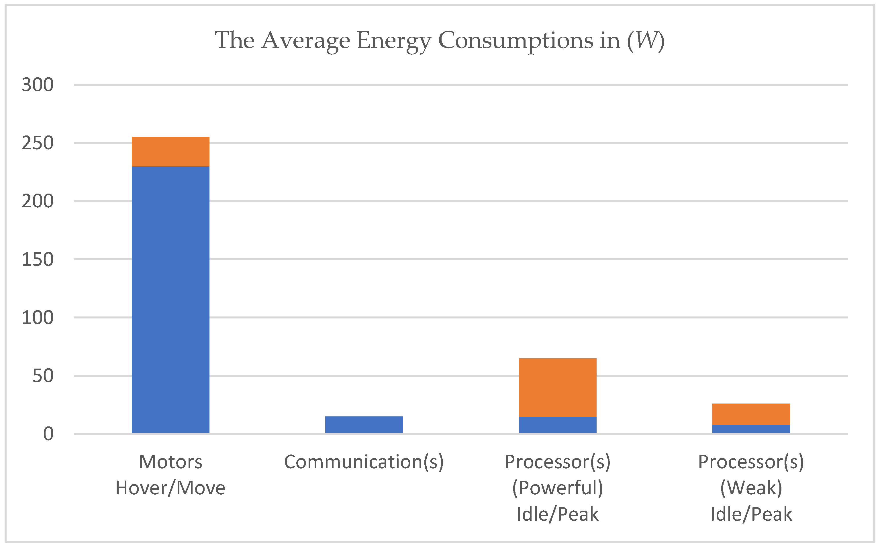
Figure 8.
Illustration of weight calculations along the path in 3 different situations, see nodes n(i). The drone is point and orientation represented, see blue full arrow line. The wind direction is represented with dashed arrow line.
Figure 8.
Illustration of weight calculations along the path in 3 different situations, see nodes n(i). The drone is point and orientation represented, see blue full arrow line. The wind direction is represented with dashed arrow line.
Description of n(1): At this node the drone has to start, accelerate to the desired velocity, reach the desired altitude (rise), and change its orientation by an angle of α(1) (rotate around x-axis). After by the given orientation on the given altitude the drone executing the distance l(1). The tall wind has to be considered in Emotors equation.
Description of n(2): In this node the drone keeps the altitude, only has to change its orientation around z-axis by an angle of α(2). In Emotors equation a side-wind has to be considered. After the drone executes the l(2) distance.
Description of n(3): In this node the drone has to change its altitude (fall to the given altitude), change the orientation by the angle α(3) around the z-axis, and the front-wind (contra wind) has to be considered in Emotors equation.
5.1.2. The Final Weighting Calculation of the Path
There are many possible routes between the START and GOAL positions. Let the index of these paths be k={1,…,p} . Then the final weighting of the selected (kth) path can be calculated:
The final execution path can be chosen based on the minimum cost function (Cf(min)), where:
Cfmin = min(sumEk)
6. Possible Graph-Search Procedures, Surveying and Comparison the Effectivity of Different Optimal Path Planning Methods
In mobile robot platforms there are several methods and procedures to achieve the desired optimal path between the given points in space. Before determining the most appropriate algorithm, or algorithms, for this particular case, the methods should be classified, and determine which, or what combinations, might be the best solutions. It is essential to make the difference between path search algorithms and the trajectory optimization methods. In the case of path search, the routes are found between the START and GOAL points of the space (if it is even existing). In most cases, this search is connected by the best possibilities, which means that the shortest or fastest path will be found. Despite path search, optimization methods are usually done by choosing some optimization goal (parameter) and the optimization algorithm is driven to get as close as possible to this goal function. The graph below shows a possible classification.
Figure 9.
UAVs Path Planning Classification.
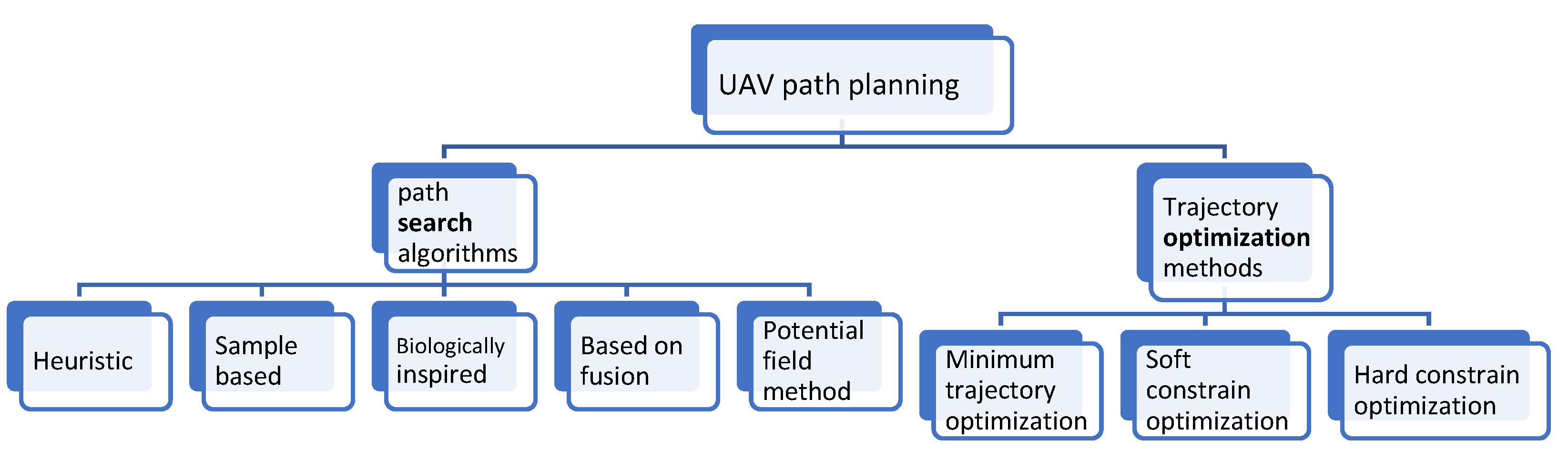
Heuristic-based path search algorithms are mostly based on graph search methods, such as: Dijsktra, A*, LifeTime Plan A* (LPA), dynamic A* (D*). These algorithms are fast and suitable for finding the shortest path between the selected positions. As of 2019, these algorithms are extended for 3D environments, and improvements (mainly of A* algorithm) can be used for variable step size and variable weights. Sum: Large amount of node calculation, poor RT performance, cannot be used in dynamic environment.
Sample-based algorithms. Two famous algorithms can be mentioned here, namely the PRM (Probabilistic RoadMap) and RRT (Rapidly-exploring Random Trees). RRT is fast, but unfortunately kinematic constrains avoidance and re-planning is not available. The path found is fast, but it can only be optimal randomly. This method has improvements such as RRT*, DDRRT, Anytime-RRT. PRM works with randomly scattered graph-nodes, which are connected to each other through some rules, and then process a graph search in space. Summary: environmental pre-information is required, the optimal path is found randomly.
Potential field (PF) algorithms. Typical algorithms for dynamic, or for multi-agent environments. It usually does not find the optimal path, but it avoids moving obstacles and other agents in space. Summary: good for dynamic PPL, but can be trapped in local minima.
Biologically inspired algorithms. Imitation of biological behavior. During the process, the building of the complex environment model is saved and based on that it proposes a powerful search method. They usually find the optimal path, but the process is relatively slow. These algorithms can be divided into 2 groups: evolutionary algorithms (Ant colony, SWARM technology); and NNs. The disadvantage of these algorithms is that sometimes suffer from the problem of premature convergence. To avoid this, the input parameters has to be stated carefully, e.g. by pre-classification. Summary: dealing with unstructured constrains. Long application time, wide search range, slow.
Algorithms Based on Fusion. These algorithms can be enrolled into 2 classes. The first class includes those that combine several PPL algorithms, integrated together, to work together to find the best path. The second class includes those that consist of several PPL algorithms, which are sequentially executed. When one algorithm completes its part, the second one starts to work immediately. As a sequential executing in a 3D environment the following sequence can be solved: 3D grid representation of the environment → using the 3D PRM (by this the obstacle-free roadmap is created) → A* algorithm to find the best path. Summary: in case of well-chosen fusion of algorithms the best PPL can be created.
Regarding optimization methods, the short characteristics of the techniques are:
Minimum trajectory optimization. Minimum trajectory optimization only ensures that the generated trajectory is smooth and dynamics, but does not constrain the trajectory itself and is suitable for unobstructed flight between two points. Summary: obstacle avoidance is problematic, but smooth trajectory dynamics are feasible.
Constrain optimization. Increase the safety constraints on flight safety. This method is divided into two main categories: hard constraints that increase the boundary value and soft constraints that increase the binding force. The hard constraint method considers all safe areas to be equivalent. The disadvantage of this is that some parts of the trajectory getting to close to the obstacle, and when the controller cannot follow the generated path, it can cause a collision, moreover the flight speed is also low. The soft constraint method applies a "push force" (using the gradient method to calculate the proximity to the obstacle) to push the trajectory away from the obstacle. Summary: hard constrain – ensuring global optimality with the convex formulation. Soft constrain – pushing the trajectory far from obstacle (safety), if there is a local minimum, the success rate and the kinematic feasibility are low.
Of course, the list is not complete, but after the study, it has to be discussed which of these methods, or what combination of these methods should be suitable for creating the energy-optimal path.
7. Calculation the Resulting Velocity and Energy Demand of the Drone
Figure 5 clearly shows that most of the energy is required by the driving motors of the drone's propellers, the other consumption is almost negligible. The power of the driving motors is closely related (directly proportional) to the speed of the drone.
Basically the forces and the energies have been calculated previously, see equations (1)-(12), now the velocities should be evaluated.
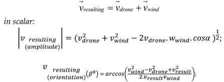
After obtaining the “wind map” of the environment the resulting velocity vector can be calculated. As seen above (see eq. (15)), the velocity directly influences the energy consumption of the drone. As a consequence, it is important to determine the correct resulting velocity. It was described in eq. (12) that Ekinetic considering the wind conditions, by the following principles, see Fig. 10.
Figure 10 a-c show that the resulting velocity of the drone is calculated from the signed vector sum of the wind speed and direction, as well as the average drone speed and direction (note: in the case of scalar calculations, the resulting velocity, -magnitude and direction-, has to be done based on well-known trigonometric (cosine theorem) equations).
Theoretically (if the drone velocity remains constant), in some cases the drone may hover in one place. The algorithm avoids this situation by making the drone change its orientation in a direction with lower resistance, and then, after travelling some distance, it turns again towards the target position. This situation will be clearly visible in the figures bellow, see Figure 11, Figure 12, Figure 13 and Figure 14
By combining eq. (16) and the power – energy relation, the following equation can be obtained:
This calculated energy is  ,
and has to be considered, and added to the final calculation of the energy
demand of the node.
,
and has to be considered, and added to the final calculation of the energy
demand of the node.
,
and has to be considered, and added to the final calculation of the energy
demand of the node. 8. Completing the Algorithm and the Flowchart of the Process
The initial idea of the project (as it is mentioned in abstract) is to use a drone to deliver small packages to hard-to-reach places (e.g. mountain rescues) and disabled people living in cities. To achieve this goal, some initial conditions has to be met.
Considered a 10x10 [km2] territory somewhere in a mountainous area, with 250[m] height from the highest terrain point. This gives the WS origin, which has to be modelled. There are very good SW tools that are able to create a 3D model of this environment based on the “google map” (here should the territory be selected) . The wind direction and wind strength sensors should be placed somewhere near (or directly on it) this territory. These sensors provide data via the IoT to the “MeteoCloud”, (a proxy server developed for Data Collection with Database and Data Management functions), which serves to create a so-called “Wind Map” of the environment.
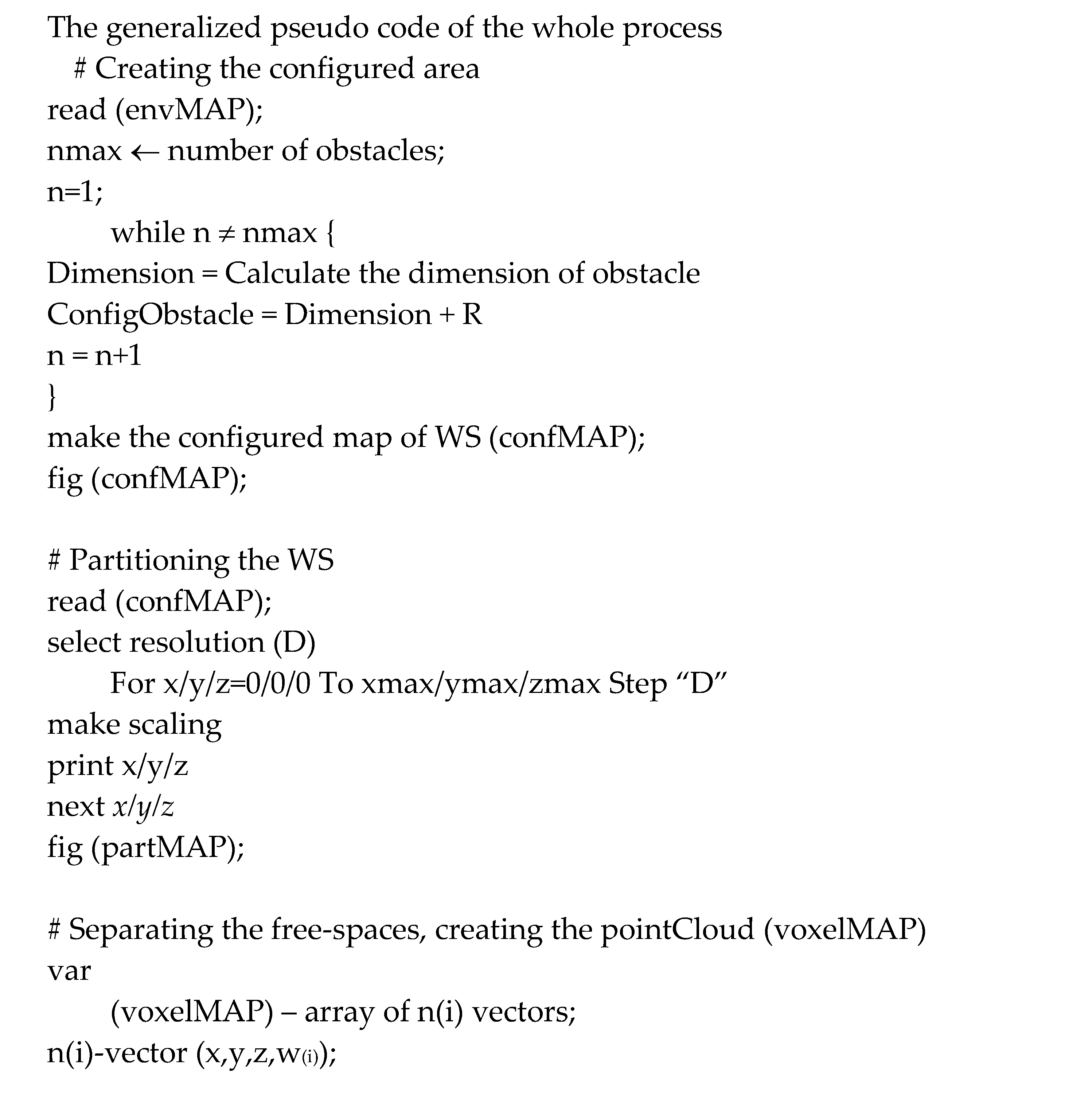
As a first step, the configuration of the WS has to be done, which means that the obstacles has to be increased by the radius of the sphere around the drone (modeling the environment). Next, WS partitioning has to be done, where the environment is divided into the cubes; then the occupied (where there are the obstacles) and free spaces are designated. Related to this process, the centre points of the free-spaces (cubes) must be designated, and based on these, the distance calculations between the centre points (edges of the graph - e(j) -) can be started. By designating the START-GOAL pair, the graph orientation can be specified. The resulting velocity of the drone can be calculated by the point represented drone (where is given the orientation and the average speed of the drone) and the wind conditions (the resulting velocity can speed up, or slow down the average velocity of the drone, based on the wind direction and speed). From the resulting velocity, the power can be calculated (eq. 15), which is directly related to the battery energy (eq. 17), through the drone’s energy consumption (eq. 12), .
As a result, the flight time over the segments (edges) of the graph is required, which is directly connected to the resulting velocity of the drone. If the wind increases the average speed, the flight time decreases and the energy consumption is less. Finally, the final execution path can be selected based on cost functions (eq. 14) of the calculated paths. The process described above, is repeated after each update of data from IoT “MeteoCloud”.
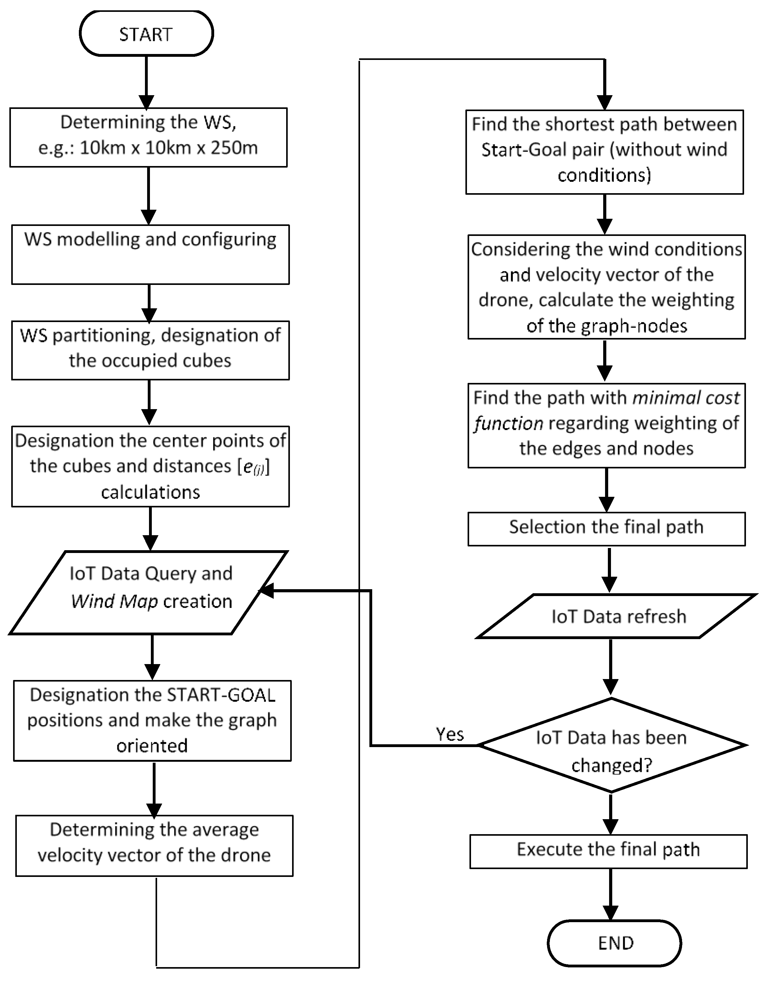
Figure 10. The Flow-chart of the whole process.
9. Results and Analysis
In order to verify the theoretical results, the authors prepared the above-mentioned (outlined) work area and examined their related assumptions.
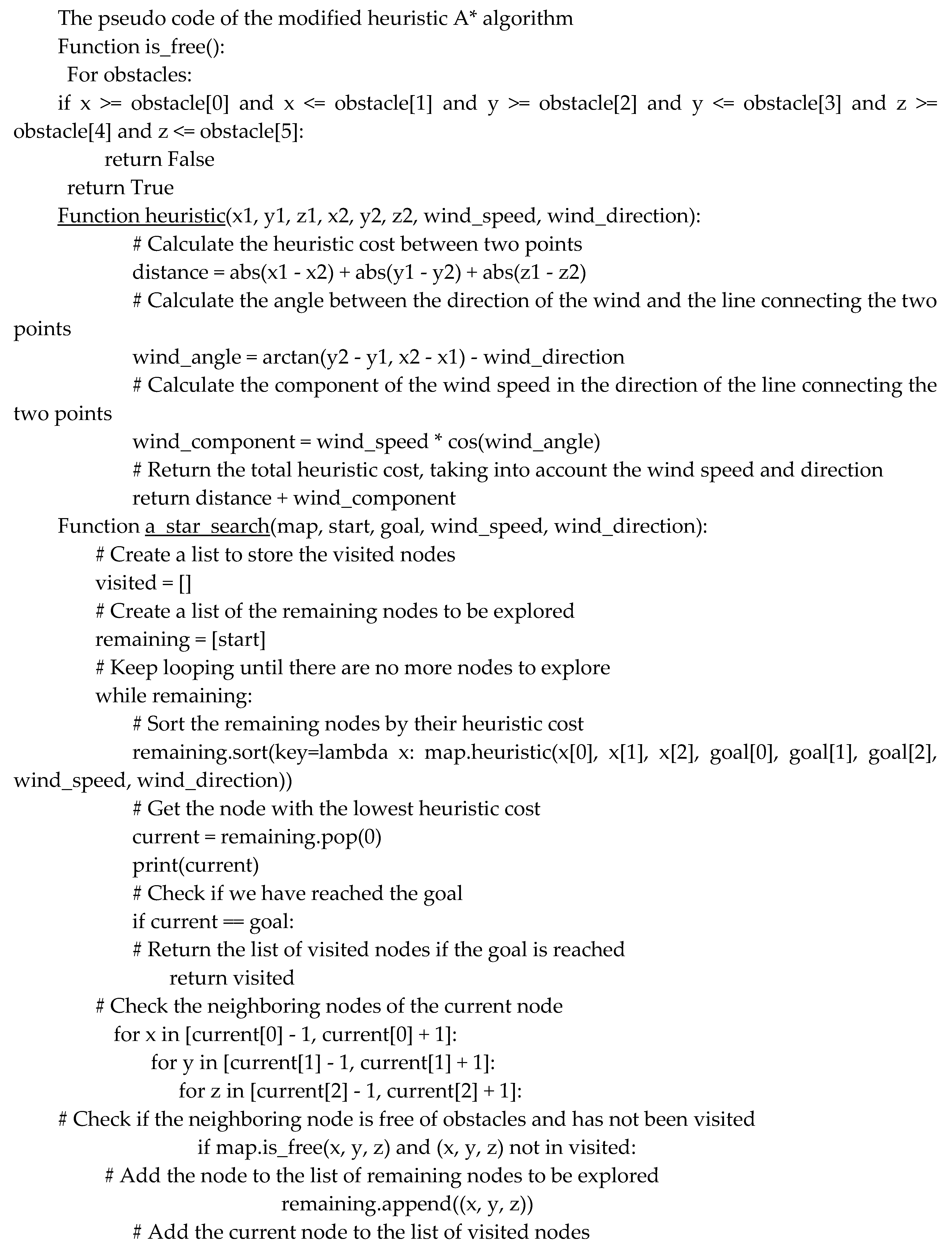
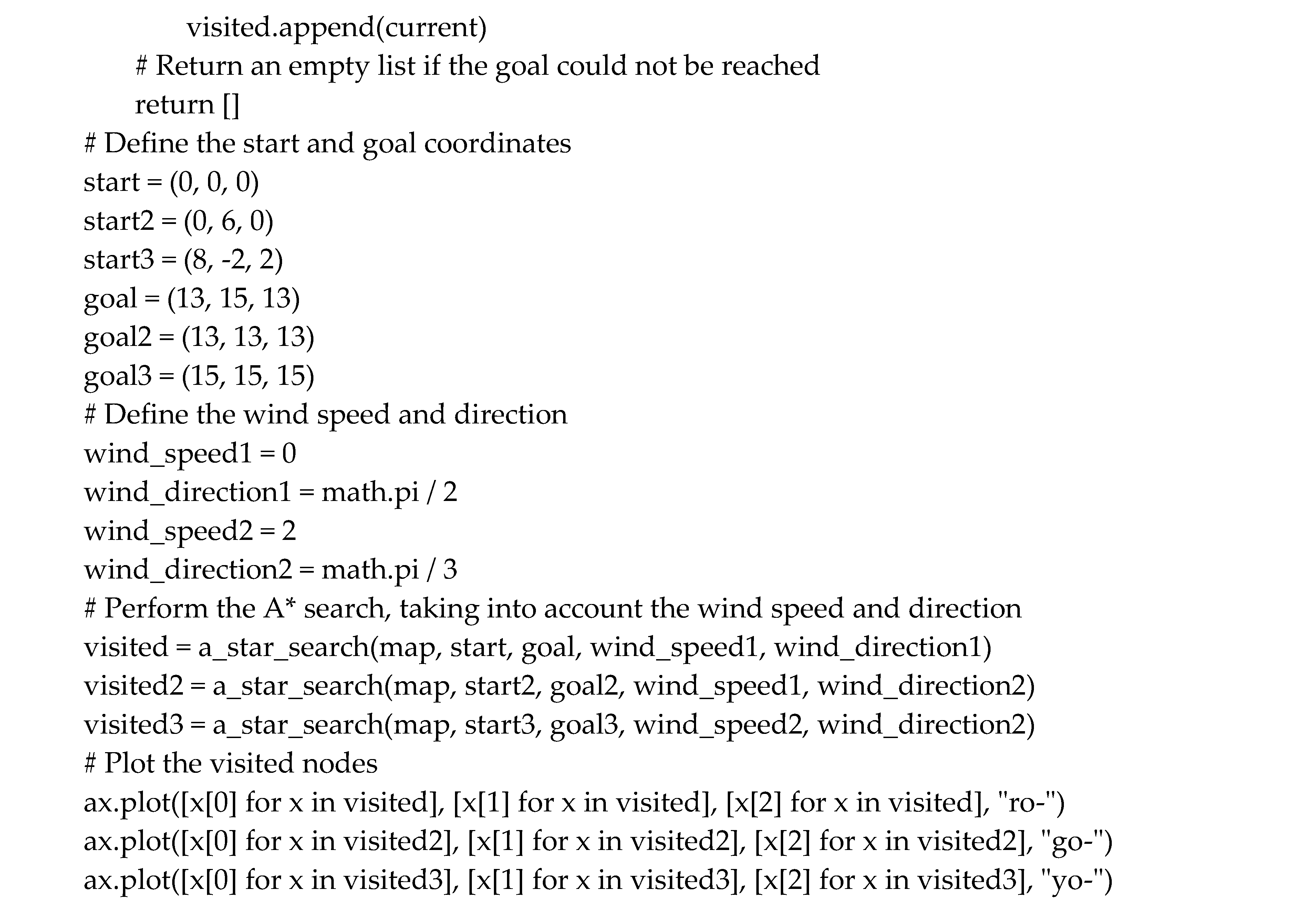
The fastest way to find the path with minimum energy demand of the drone, is the heuristic A* search method. In this particular case, the basic A* method is extended by the wind conditions, and the weighting of the edges and the nodes is introduced based on the energy demands of the path-segments. In the first step, the modelled work space map has to embedded in the system, and then the graph search has to be executed on the given environment.
First, the class Map is created and embedded in the search algorithm. It has a function called free() that checks if a point in 3D space is occupied or free. It also has a function heuristic() that calculates the absolute value of the distance between current and final points (x,y,z). It also calculates the weighting of the wind from given parameters. The A_star_search() function itself goes from point to point and checks if current point is a goal, until it reaches the final point. It uses the function heursitic()to find the optimal neighbour points. The visited nodes are saved in an array and can be represented visually. The above described algorithm considers three different paths under three different wind conditions, according to Fig. 10. The final results of the above described path planning processes can be seen in the figures bellow, see Figs. 11-13, and 14. The pseudo codes of the program are given in Appendices A and B.
10. Conclusions
Originally, this study focused on the PPL processes using evolutionary algorithms, such as NN, and GA-based PPL processes. Unfortunately, these methods are very limited in case of dynamic weighting, because they are highly dependent on the training (or new population generation) time and the update frequency of the weights. Simply, during training, the weights can change several times, and the selected path will not be the optimal and current one. Based on these studies, the dynamic and Real-Time PPL methods seem to be appropriate, and this is how the heuristic A* algorithm is selected.
Basically a modified A* algorithm was used by the
authors, because in the classic algorithm the edges are weighted and the
optimal path is searched based on a cost function. In this modification, not
only the edges but also the nodes are weighted, and the algorithm steps from node
to node, selecting the branch to the next node based on the actual weight
(which is calculated and evaluated) at each node. A good example can be seen on
Fig. 13 (see, yellow path), where the drone has to fly in front-wind and
“sailing” between nodes to achieve minimum energy use. Basically,
it is a very complex system, and for this reason it is divided into
sub-programs (procedures) and their operation is interconnected and/or
interlinked. The system using two Databases (DBs): 1. “MeteoCloud” –
where the IoT data of the meteo stations is uploaded. The wind map for the
selected Working Space is created from this DB. 2. is the “PointCloud”
of geographical data of the selected WS. After partitioning the WS, the points
are represented by the center-points of the cubes, and these points are also
the nodes of the graph (of course, only in free-spaces). These points (nodes) are
basically vectors (arrays) containing coordinates and calculated weights, 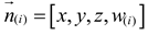 .
.
. Author Contributions
Conceptualization, I.N. and E.L.; methodology, I.N.; software, I.N. and E.L.; formal analysis, I.N.; investigation, I.N and E.L.; resources, I.N..; writing—original draft preparation, I.N. and E.L.; writing—review and editing, I.N. and E.L.; supervision I.N. and E.L. All authors have read and agreed to the published version of the manuscript.
Funding
The research was funded by the Óbuda University Open Access Publication Support Foundation.
Institutional Review Board Statement
Not applicable.
Informed Consent Statement
Not applicable.
Data Availability Statement
The data presented in this study are available on request from the corresponding author. The data are not publicly available due to this is an ongoing research.
Acknowledgments
This work was supported by the Fuzzy Systems Scientific Group at the Bánki Donát Faculty of Mechanical and Safety Engineering of Óbuda University.
Conflicts of Interest
The authors declare no conflict of interest.
Appendix A
Appendix B

References
- Gušavac, B.A.; Martić, M.; Popović, M.; Savić, G. Agricultural Route Efficiencies, based on Data Envelopment Analysis (DEA). Acta Polytechnica Hungarica, Vol. 20, No. 10, (2023), pp. 73-88.
- Anatomy of A Drone - What's inside a DJI Phantom Drone, https://www.dronefly.com/the-anatomy-of-a-drone (accessed on 04. November 2022).
- Drone design – Calculations and Assumptions, https://tytorobotics.com, (accessed on 22 October 2022).
- Working Principle and Components of Drone, https://cfdflowengineering.com/working-principle-and-components-of-drone/ , (accessed on 22 October 2022).
- Working Principle and Components of Drone, https://cfdflowengineering.com/working-principle-and-components-of-drone/ , (accessed on 22 October 2022).
- Working Principle and Components of Drone, https://cfdflowengineering.com/working-principle-and-components-of-drone/ , (accessed on 22 October 2022).
- Pandya, G. Basics of Unmanned Aerial Vehicles, Publisher: Notion Press, CIT Colony, Mylapore, India, 2021, ISBN 978—1-63745-387-2.
- Abel J.P. Gomez; I. Voiculescu; J. Jorge; B. Wyvill; C. Galbraiht Spatial Partitioning Methods. In Implicit Curves and Surfaces: Mathematics, Data Structures and Algorithms, Publisher: Springer, London, 2009; pp. 187-225. [CrossRef]
- Sabry, F. Exploring Binary Space Partitioning: Foundations and Applications in Computer Vision. In Binary Space Partitioning, Publisher: One Billion Knowledgeable, 2024.
- Fabrice Jaillet, Claudio Lobos. Fast Quadtree/Octree adaptive meshing and re-meshing with linear mixed elements. In Engineering with Computers, ff10.1007/s00366-021-01330-wff. ffhal-03161623, 2021.
- MathWorks, octree - partitioning 3D points into spatial subvolumes, https://www.mathworks.com/matlabcentral/fileexchange/40732-octree-partitioning-3d-points-into-spatial-subvolumes, (accessed on 04. November 2022).
- MathWorks, exportOccupancyMap3D, https://www.mathworks.com/help/nav/ref/exportoccupancymap3d.html, (accessed on 04. November 2022).
- Sanches-Lopez, J. L.; Wang, M.; Olivares-Mendez, M.A.; Molina, M.; Voos, H. A Real-Time 3D Path Planning Solution for Collision-Free Navigation of Multirotor Aerial Robots in Dynamic Environments, Journal of Intelligent & Robotic Systems 2018, Vol. 93, pp. 33-53. [CrossRef]
- Lifen, L.; Ruoxin, B. S.; Shuandao, C. L.; Jiang, D.W. Path planning for UAVS Based on Improved Artificial Potential Field Method through Changing the Repulsive Potential Function; In Proceedings of the 2016 IEEE Chinese Guidance, Navigation and Control Conference, https:/doi.org/10.1109/CGNCC.2016.7829099, 2016, pp. 2011-2015. [CrossRef]
- Chen, X.; Zhang, J. The Three-dimension Path Planning of UAV Based on Improved Artificial Potential Field in Dynamic Environment; In Proceedings of the 2013 Fifth International Conference on Intelligent Human-Machine Systems and Cybernetics, 2013, pp. 144-147. [CrossRef]
- Boyu Zhou, Fei Gao, Jie Pan, and Shaojie S. Robust Real-time UAV Replanning Using Guided Gradient-based Optimization and Topological Paths; In Proceeding of the 2020 IEEE International Conference on Robotics and Automation (ICRA), Paris, France, 2020, pp. 1208-1214. [CrossRef]
- F. Samaniego, J. Sanchis, S. Garcia-Nieto, R. Simarro. Smooth 3D Path Planning by Means of Multiobjective Optimization for Fixed-Wing UAVs. MDPI, Electronics 2020, 9(1), 51. [CrossRef]
- Sanches-Lopez J.L., Wang M., Olivares-Mendez, Miguel A., Molina, Martin, Voos, Holger A Real-Time 3D Path Planning Solution for Collision-Free Navigation of Multirotor Aerial Robots in Dynamic Environments Journal of Intelligent & Robotic Systems, 2019. [CrossRef]
- Francis Colas, Srivatsa Mahesh, François Pomerleau, Ming Liu, Roland Siegwart. 3D path planning and execution for search and rescue ground robots. In IEEE/RSJ International Conference on Intelligent Robots and Systems (IROS), 2013, Tokyo, Japan. pp. 722–727. hal-01143103, 2015. [CrossRef]
- Ahmed G., Sheltami T., Mahmoud A., Yasar A. Energy-Efficient UAVs Coverage Path Planning Approach. CMES, 2023, vol.136, no.32022, pp. 3239-3263. [CrossRef]
- EASA. Drone Regulatory System, Understanding European Drone Regulations and the Aviation Regulatory System, EU and MS regulatory governance. https://www.easa.europa.eu/en/domains/drones-air-mobility/drones-air-mobility-landscape/Understanding-European-Drone-Regulations-and-the-Aviation-Regulatory-System (accessed on 16. jun 2024.).
- Thomas Kirschstein. Comparison of energy demands of drone-based and ground-based parcel delivery services. Elsevier, Transportation Research Part D Vol 78, (2020) 102209. [CrossRef]
- Çabuk, U.C.; Tosun, M.; Jacobsen, R.H.; Dagdeviren, O. A Holistic Energy Model for Drones. In 2020 28th Signal Processing and Communications Applications Conference (SIU), Gaziantep, Turkey, 2020, pp. 1-4. [CrossRef]
- Al-sudany, H.N.; Lantos, B. Extended Linear Regression and Interior Point Optimization for Identification of Model Parameters of Fixed Wing UAVs. Acta Polytechnica Hungarica, Vol. 21, No. 6, (2024), pp. 69-88.
Figure 3.
Forces, moments and torques used in drone flights (equations (1)-(7)), with the drone coordinate system, and roll, pitch, yaw movements were adopted from [4].
Figure 3.
Forces, moments and torques used in drone flights (equations (1)-(7)), with the drone coordinate system, and roll, pitch, yaw movements were adopted from [4].
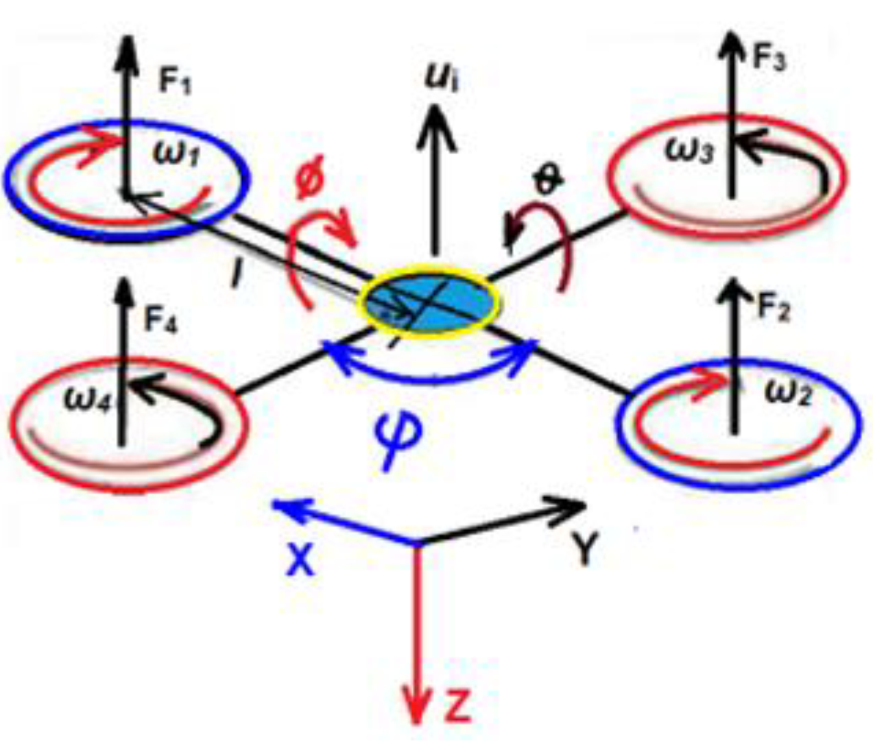
Figure 4.
The idealized UAV flight pattern, where C1 and C2 areas are energy consuming, while S area is energy saving region [22].
Figure 4.
The idealized UAV flight pattern, where C1 and C2 areas are energy consuming, while S area is energy saving region [22].
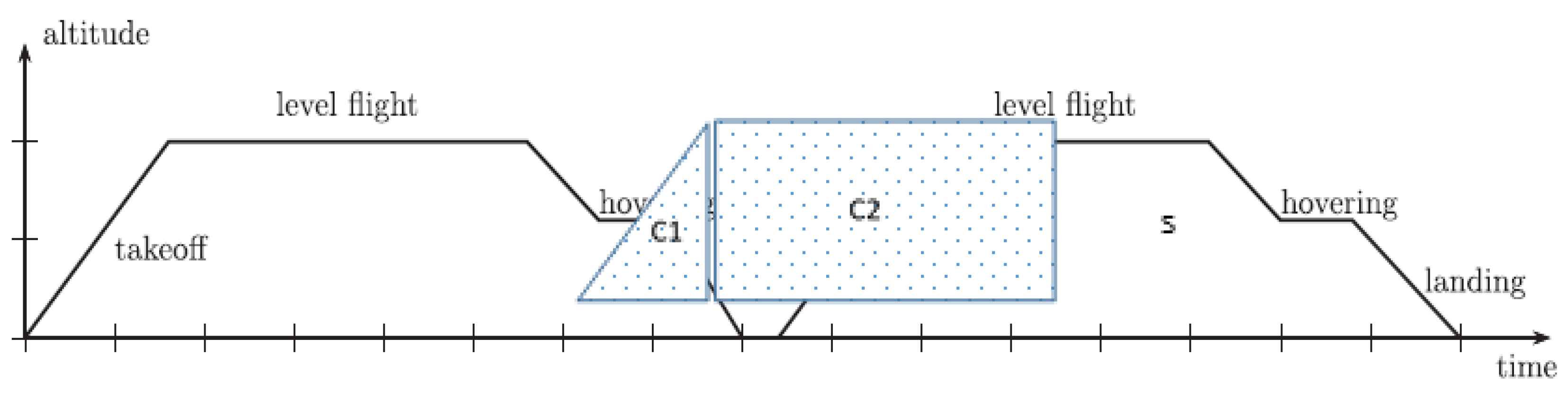
Figure 6.
The scaled partitioned sample WS, with occupied blocks (blue dots) and Free Spaces (FSs).
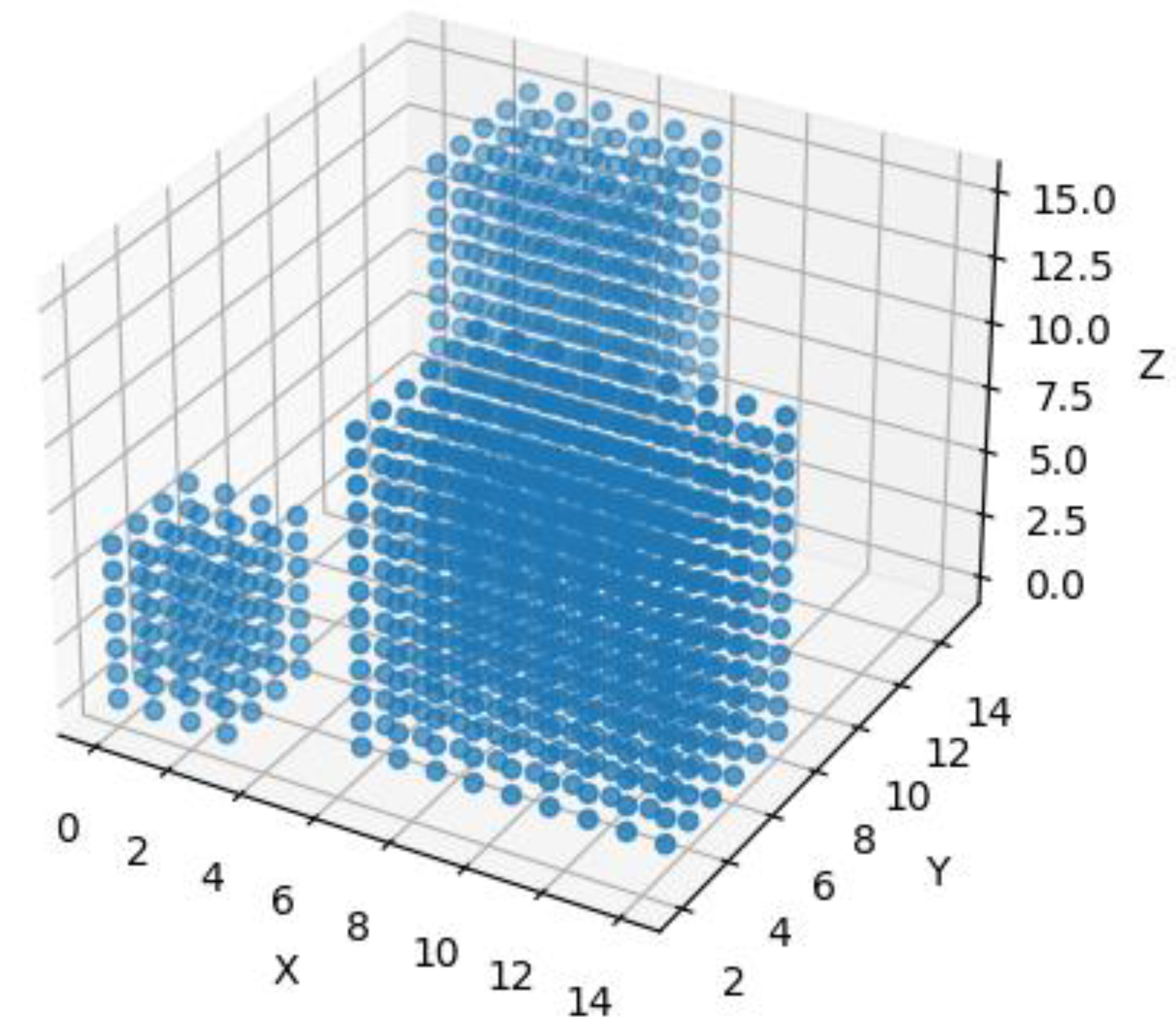
Figure 7.
Creation of the graph-like, (topological) map of the space, where the center points of the FS blocks are connected. Where the connecting line crosses (or touch) the occupied block (see red line) the connection is not possible.
Figure 7.
Creation of the graph-like, (topological) map of the space, where the center points of the FS blocks are connected. Where the connecting line crosses (or touch) the occupied block (see red line) the connection is not possible.

Figure 10.
The resulting velocity calculation of the drone. (a) tall-wind; (b) side-wind; (c) front-wind. The wind direction is represented by the dashed-arrow lines; the resulting (calculated) velocity vector of the drone is represented by red full-arrow line; the initial velocity and orientation of the drone is represented by blue full-arrow line. .
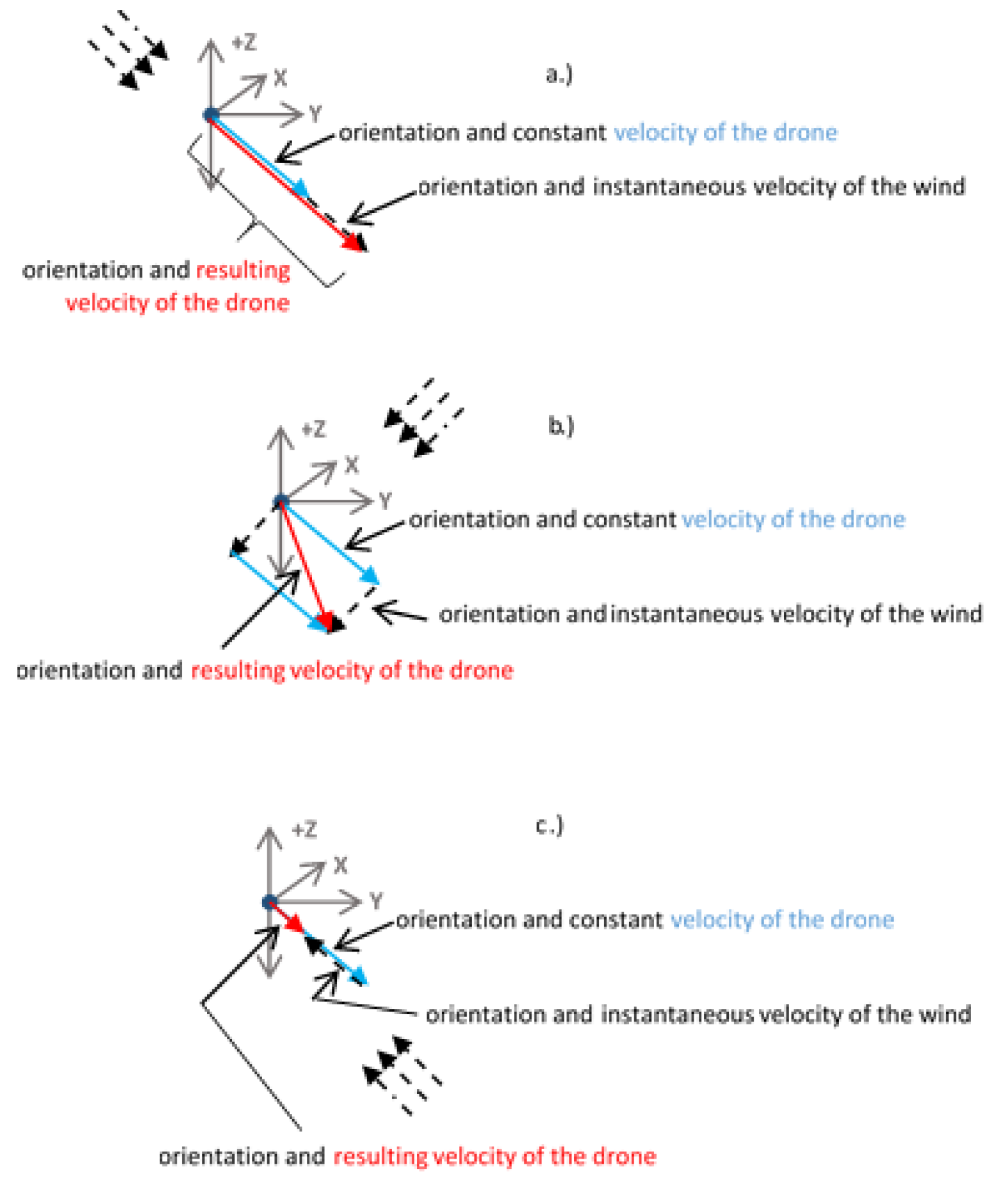
Figure 11.
The calculated optimal trajectory from START (left bottom corner) to GOAL positions in case of tall-wind situation. .
Figure 11.
The calculated optimal trajectory from START (left bottom corner) to GOAL positions in case of tall-wind situation. .
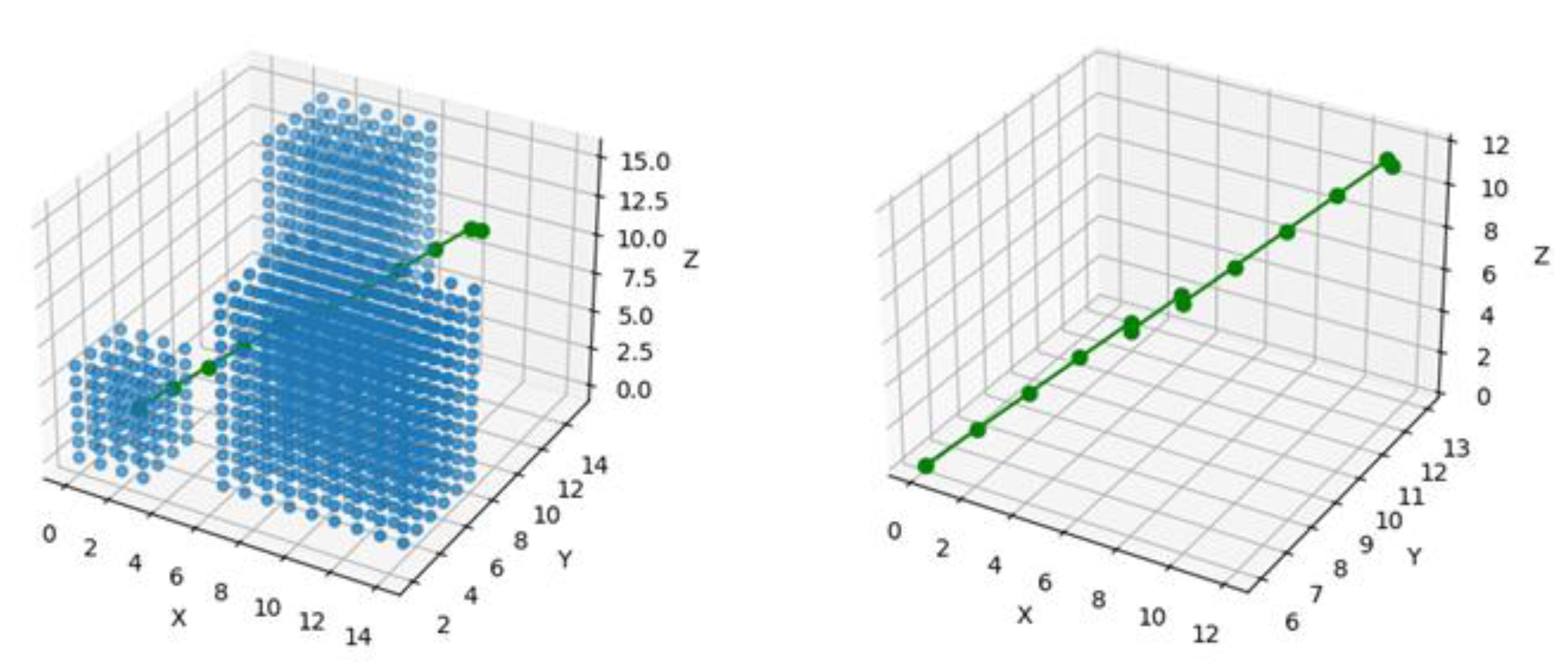
Figure 12.
The calculated optimal trajectory from START (left bottom corner) to GOAL positions in case of side-wind situation. .
Figure 12.
The calculated optimal trajectory from START (left bottom corner) to GOAL positions in case of side-wind situation. .
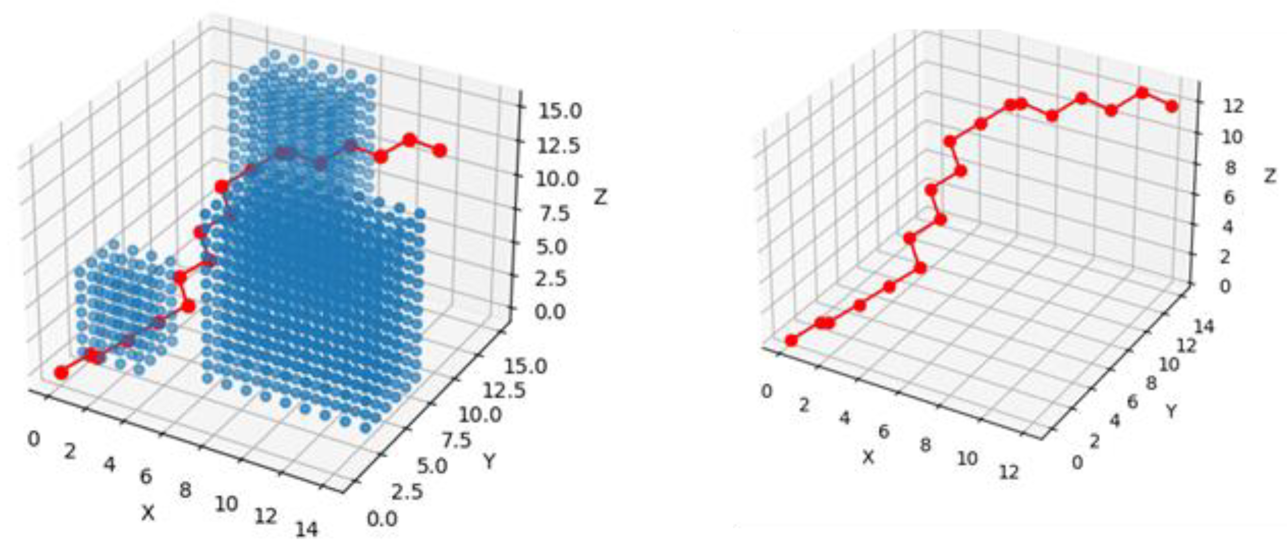
Figure 13.
The calculated optimal trajectory from START (left bottom corner) to GOAL positions in case of front-wind situation. .
Figure 13.
The calculated optimal trajectory from START (left bottom corner) to GOAL positions in case of front-wind situation. .
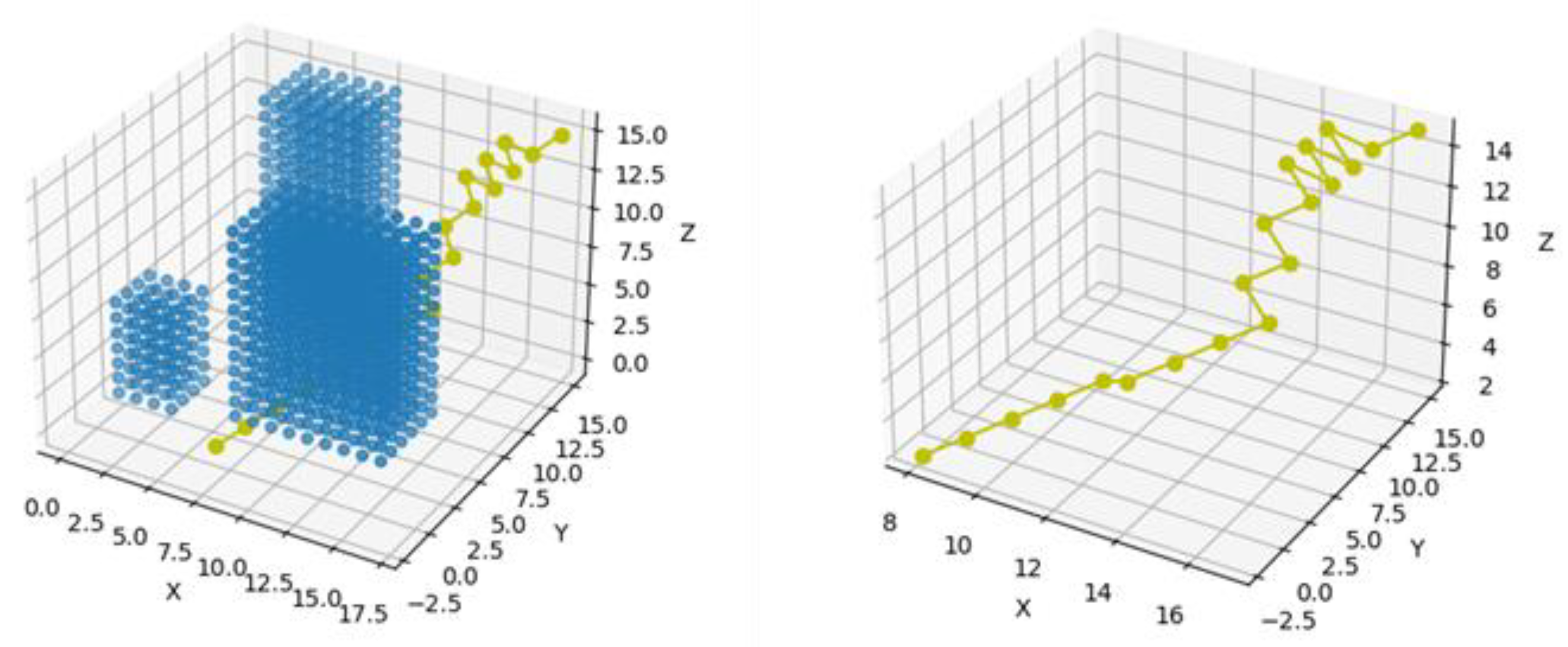
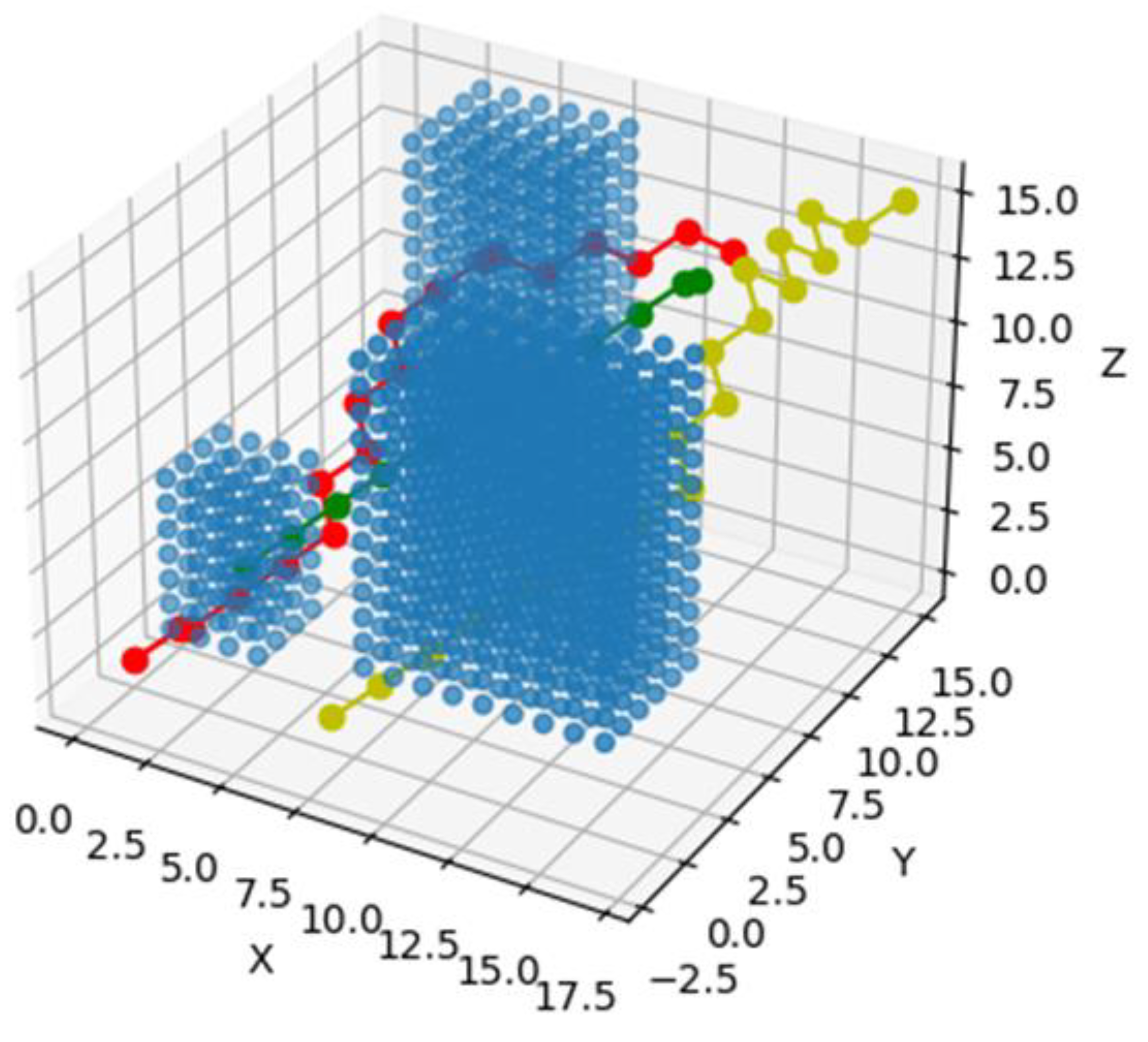
Figure 14.
The sum of calculated optimal trajectories from START (left bottom corner) to GOAL positions. .
Figure 14.
The sum of calculated optimal trajectories from START (left bottom corner) to GOAL positions. .
Disclaimer/Publisher’s Note: The statements, opinions and data contained in all publications are solely those of the individual author(s) and contributor(s) and not of MDPI and/or the editor(s). MDPI and/or the editor(s) disclaim responsibility for any injury to people or property resulting from any ideas, methods, instructions or products referred to in the content. |
© 2024 by the authors. Licensee MDPI, Basel, Switzerland. This article is an open access article distributed under the terms and conditions of the Creative Commons Attribution (CC BY) license (http://creativecommons.org/licenses/by/4.0/).
Copyright: This open access article is published under a Creative Commons CC BY 4.0 license, which permit the free download, distribution, and reuse, provided that the author and preprint are cited in any reuse.


