Submitted:
11 July 2024
Posted:
12 July 2024
You are already at the latest version
Abstract
The spin-torsion theory is a gauge theory approach to gravity that expands upon Einstein's general relativity (GR) by incorporating the spin of microparticles. In this study, we further develop the spin-torsion theory to examine spherically symmetric and static gravitational systems that involve free-falling macroscopic particles. We posit that the quantum spin of macroscopic matter becomes noteworthy on cosmic scales. We further assume that the Dirac spinor and Dirac equation adequately capture all essential physical characteristics of the particles and their associated processes. A crucial aspect of our approach involves substituting the constant mass in the Dirac equation with a scale function, allowing us to establish a connection between quantum effects and the scale of gravitational systems. This mechanism ensures that the quantum effect of macroscopic matter is scale-dependent and diminishes locally, a phenomenon not observed in microparticles. For any given matter density distribution, our theory predicts an additional quantum term, the quantum potential energy (QPE), within the mass expression. QPE induces time dilation, distance contraction, and thus mimics a gravitational well. When applied to cosmology, our theory yields a static cosmological model. The QPE serves as a counterpart to the cosmological constant introduced by Einstein to balance gravity in his static cosmological model. The QPE also offers a plausible explanation for the origin of the Hubble redshift (traditionally attributed to the universe's expansion). The predicted luminosity distance-redshift relation aligns remarkably well with SNe Ia data from the cosmological sample of SNe Ia. In the context of galaxies, QPE functions as the equivalent of dark matter. The predicted circular velocities align well with the rotation curve data from the SPARC (Spitzer Photometry and Accurate Rotation Curves database) sample. Importantly, our conclusions in this paper are reached through a conventional approach, with the sole assumption of the quantum effects of macroscopic matter on large scales, without the need for additional modifications or assumptions.
Keywords:
alternative theories of gravity
; dark matter
; dark energy
; cosmology
; galactic dynamics
; spacetime algebra
; gauge theory of gravity
1. Introduction
The primary challenge facing the current theory of gravity, the Einstein-Newton theory, lies in the unresolved mysteries of dark matter and dark energy. To date, there is a lack of direct observational evidence confirming the existence of these enigmatic components. Extensive efforts are being made to address such a topic. On the theoretical front, much attention is directed towards modifying or extending the Einstein-Newton theory of gravity to align with astronomical observations. For instance, one can enhance the standard Lagrangian in General Relativity by incorporating higher order curvature corrections [4,5,28,31,32,40], or formulate non-linear Lagrangians [8,16]. Other relevant examples include MOdified Newtonian Dynamics (MOND) [15,38] and its relativistic version [1], as well as conformal gravity [33,34].
In this paper, we explore the concept of quantum spacetime on cosmic scales as a potential alternative to dark matter and dark energy. This research represents a significant extension of our previous study [10]. Rather than relying on previous assumptions, we explicitly propose the scale-dependent quantum properties of spacetime. This proposition is motivated by our interest in potentially moving away from the notion of a preferred absolute spacetime for the universe, as implied by General Relativity (GR) and illustrated in the standard CDM cosmology.
Before going further, it is imperative to clarify our actual motivation in order to prevent any possible misunderstandings. For ease of references, we categorize the universe into three distinct classes based on spatial scales: the cosmic scale (encompassing galaxies to the entire universe), the macroscopic scale (ranging from everyday life to the size of the solar system), and the microscopic scale (where quantum mechanics becomes significant as is well known). According to the mainstream view, the quantum effect for objects at the macroscopic and cosmic scales can be safely disregarded due to their large mass. This is known as the classical limit. According to our assumption, however, the quantum effects are dependent on the scale of the gravitational system considered, and the "classical limit" is only reached at macroscopic scale. In other words, quantum effects are significant not only at microscopic scale but also at cosmic scale, and can be ignored only at macroscopic scale. Intuitively, when we study cosmology, observers who perceive distant galaxies in the universe, would expect them to exhibit the quantum behavior resembling that of microscopic particles, due to their distant locations. As for the galactic dynamics, the quantum effect should also be taken into account for galaxies, although in the central part it can be ignored according to our assumption.
We will illustrate the integration of our assumption with the Einstein equations. It is natural for us to generalise the Dirac theory to describe the matter content. We present a direct application of the covariant Dirac equation without any modifications to study radially symmetric and static gravitational systems, such as galaxies and the entire universe, along with an explanation of the underlying mechanism that allows us to do so. We need the stress-energy tensor derived from the Dirac theory formulated as a new kind of hydrodynamics. Prior to incorporating the stress-energy tensor derived from Dirac theory into the Einstein equation, it is crucial to explicitly distinguish between its spin-free component (representing the classical ideal fluid) and the spin component (depicting the quantum potential energy). We have observed that without this separation, as demonstrated in prior research [10], the resulting Einstein equation is unable to accurately depict the pressure-free ideal fluid when the spin is locally negligible. By successfully solving the Einstein field equations, we have discovered some important conclusions that have not appeared in the literature.
There are two approaches to interpreting quantum mechanics. The first is the standard view, which asserts that micro particles cannot have continuous trajectories and that non-commuting observables (such as position and momentum) must satisfy the uncertainty principle. The second approach is known as the causal interpretation, which posits that each microparticle has a continuous trajectory and replaces the uncertainty principle with the concept of quantum potential[2,27]. Both approaches yield equivalent predictions for experimental results. However, the causal interpretation, particularly in its geometric algebra (GA) version, provides profound insights into the quantum nature of spacetime and matter [20,22,23,24]. In this paper, similar to our previous work, we utilize the spacetime algebra (STA) [12,19,24] as our mathematical language. STA is constructed from a Minkowskian vector space and provides a straightforward geometric understanding of Dirac theory. It bridges a natural link to classical mechanics, and for expressing Dirac theory with observables, it offers enhanced computational efficiency and capabilities [22] when compared to the tensor analysis method [43]. The fundamentals of STA are outlined in Appendix A. In the STA version of Dirac theory, known as real Dirac theory, Hestenes identified the complex number present in the matrix version of Dirac theory as the spin plane [20]. Furthermore, since the complex number is always accompanied by the Planck constant ℏ, a rigorous derivation of the Schrodinger theory from the Pauli or Dirac theory implies that the Schrodinger equation describes an electron in an eigenstate of spin, rather than, as commonly believed, an electron without spin [21]. Correspondingly, there are two gauge theories of gravity concerning our research work: one is the tensor analysis approach [17], and the other is gauge theory gravity (GTG) developed by the Cambridge group using STA [29]. The two theories are nearly equivalent, but the latter is conceptually clearer and technically more powerful for comprehending and calculating the challenges encountered in quantum mechanics and gravity. Therefore, we choose to adopt GTG in this paper. The fundamentals of GTG and its applications to spin- particles are summarized in Appendix C.
It is now widely acknowledged that the quantum random motion of spin- particles can be fully described by its spin. In the presence of gravity, the spin gives rise to the torsion of spacetime [12,13,17,25,26,29]. For massive fermions, such as electrons and neutrons, the mass will always appear in the phase factor of the solutions of the wave equations. When gravity matters, this mass dependence remains. Consequently, it is generally believe that the gravity effect is not purely geometric at the quantum level. Hence the immediate question is, how can we reconcile, if possible, the contradiction between the quantum effect and the requirement of geometric description of gravity? For microparticles, reconciling this contradiction is indeed impossible. However, in this study, we propose that the scale-dependent quantum effect on macroscopic matter only becomes significant on cosmic scales. Locally, on a macroscopic scale, the large mass m of each particle, or equivalently, the small value of the number density of the fluid, guarantees what is known as the classical limit, allowing for a geometric description of the gravitational effect on macroscopic matter. The remaining question is, what mechanism ensures that quantum effects are significant at cosmic scales while being negligible at macroscopic scales?
The answer to this question is not intricate, but rather subtle. The specifics will be provided later, but for now, we will outline the main concepts behind the mechanism. Our analysis commences with an examination of the Dirac theory within various inertial frames [22]. Generally, the Lorentz invariant Dirac spinor is defined in spacetime as
where is a scalar, represents the proper probability density and is a rotor (Lorentz rotation) satisfying . In Dirac theory, the parameter is intriguing. It is noteworthy that the states of plane-wave particle have , while those of antiparticle have . In this paper, we aim to utilize the spinor for describing free-falling macroscopic particles, hence it is logical to set throughout. Therefore, we adopt [10]
The Dirac equation is
where ℏ is Planck constant. This equation describes a single spin free particle with a fixed mass m and the probability density . If we interpret as the number density of a fluid, then we refer to as the mass density. It is convenient to define a spin density trivector as (note that it is denoted with in Appendix B)
We show in Appendix B that, the stress-energy tensor for the spinor field is
where v is the current velocity. When (this is the classical limit), this equation becomes the stress-energy tensor of a pressureless ideal fluid without spin
When applying these results to gravitational systems, we simply need to replace ∇ with the covariant derive symbol D, while all other quantities remain gauge-invariant. As such, the classical limit (also known as the short wave approximation) refers to the fact that the contribution of the spin to the stress-energy is negligible. Clearly, the magnitude of the spin is determined by the number density . Therefore, an alternative interpretation for the classical limit is that the value of the number density, , is ignorably low, whereas the significant quantum effect arises when is sufficiently high. For any fixed mass density , the spin can be determined via . This freedom strongly indicates that in order to incorporate the scale-dependent quantum effect on scales, we can replace the mass m in the Dirac equation with a mass function that depends on the spatial scale of the system, denoted as . The mass function naturally satisfies the condition that, when , then , corresponding to the macroscopic scale. Conversely, when , then S becomes a dependent quantity related to the constant density of the universe. The intermediate functional form of , which plays a crucial role in the study of galaxies, can be determined through observations. Consequently, we can employ the Dirac equation in the presence of gravity without any modifications, as there are no derivatives of involved in our calculations. The properties of the mass function only need to be discussed in the final results.
It is important to explicitly acknowledge that when applying the Dirac equation to gravitational systems on cosmic scales, we shall show in Section 3 that the anisotropy of the spin density adheres to the symmetric properties of mass density . This fact applies only to macroscopic matter according to our assumption, where the gravitational effect is geometric throughout the spacetime manifold and, furthermore, the mass density and the spin density have already been averaged and must satisfy the condition that the quantum effect vanishes locally. On the other hand, when considering electrons, the anisotropy of spin must be taken into account in all cases, as the gravitational effect is not purely geometric. Thus the quantum effect can never disappear locally, as is commonly understood [6,7,9,42].
The subsequent sections present the examination of radially-symmetric and static gravitational systems based on our new postulation in Section 2, the applications of our findings to cosmology and galaxies in Section 3, and the summarized conclusions and discussions in Section 4. We employ natural units () throughout except stated otherwise.
2. radially Symmetric Gravitational Systems
We want to investigate the quantum nature of spacetime on cosmic scales, with the main subjects of concern being galactic dynamics and cosmology. Traditionally, the pressureless ideal fluid is a good model for both galactic dynamics and mater-dominated era cosmology. In both scenarios, matter experiences free-fall in a gravitational field and is characterized by the density distribution and velocity field , where x represents the position vector in spacetime. This model is usually known as collapsing dust. In gravitational systems, it is widely recognized that a static state can only be sustained when there is a substantial gravitational potential well, as observed in galaxies. However, in the realm of cosmology, the homogeneous and isotropic distribution of matter across the entire universe renders static solutions non-existent.
Nevertheless, the introduction of quantum effects on cosmic scales fundamentally alters the situation.
The Dirac theory for radially symmetric gravitational systems is to be investigated using Gauge Theory Gravity (GTG). The latter is constructed such that the gravitational effects are described by a pair of gauge fields, and , defined over a flat Minkowski background spacetime [29], where x is the STA position vector and is usually suppressed for short. Luckily, the majority of the necessary results for our present study have already been derived in prior works [13,29]. We have summarised them in Appendix C.
Let us consider a radially-symmetric and static gravitational system composed of free-falling particles with the identical mass m. We make the assumption that the Dirac spinor defined in (2) can fully capture all the essential physical aspects of the system if it satisfies the Dirac equation
We interpret as the number density and as the mass density. We adopt defined in (4) as the spin density trivector for the gravitational system. So there are four variables, namely m, , and S, that can be used to describe the gravitational system. However, only two of them are independent, as they must satisfy the conditions and . In this paper, we will eliminate m and retain the other three variables. Among them, the relationship between and can be further determined through observations by assuming a specific form for the mass function . Once this is done, we are left with only one variable, which is the mass density . Therefore, if we are given the mass density of a gravitational system, we can predict the entire set of results, including the quantum effects.
Now we define a set of spherical coordinates. From the position vector of the flat spacetime
we obtain the basis vectors as follows
Since and are not unit, we define
With these unit vectors, we further define the unit bivectors (relative basis vectors for )
These bivectors satisfy
As in our previous paper [10], we attempted to analyze static systems initially. The set of field that satisfies the spherically-symmetric and static matter distribution is assumed to take the form [12,29]
where , and are all function of r only. We could have tried a form , but it is more reasonable to set to zero, which is referred to as the `Newtonian gauge’ [29].
The subsequent steps of this study can be summarized as follows:
where the metric is introduced to compare our results with those predicted by general relativity (GR) and to provide the conventional approaches for subsequent applications. Notably, and can be decomposed into torsion-free components and torsion components. This decomposition allows for the recovery of classical predictions of GR when the impact of torsion is insignificant. Conversely, given the extensive research on these classical predictions available in the existing literature, we can easily incorporate the torsion terms into the classical results when we deem them to be significant. This allows us to leverage the decompositions and enhance our understanding of the phenomena under consideration.
By solving Equation (A37), we can obtain the solusion for [29], the result is
where
denotes the torsion-free component of , and the new functions G and F are also all functions of r only. From the field, for any bivector B, its strength tensor can be obtained directly from Equation (234) [13,29], the result is
where
denotes the torsion free component of , with the understanding that , and are given by
From Eqs.(16) and (17), the Ricci tensor and Ricci scalar are given by
where
and
denote the torsion free components of and , respectively.
In order to solve Einstein equation Equation (), we need to know given by Equation (242). Noting that , we find that
The terms should be derived from the Dirac equation (7). Nevertheless, as elaborated in our previous paper [10], the use of this stress-energy tensor prototype can be misleading when applied to gravitational systems consisting of macroscopic bodies. This is because, as S approaches zero, the tensor defined in (22) also approaches zero. This contradicts our expectation that as S tends to zero, should represent a tensor describing the pressureless ideal fluid.
An appropriate representation of the stress-energy tensor for our specific needs involves decomposing it into two components: one that characterizes the classical pressure-free ideal fluid and another that accounts for quantum effects. By substituting ∇ with D, we can rephrase equation (198) and express as,
where we have replaced v with due to the retained gauge freedom to perform arbitrary radial boosts in restricting the function [12,29].
The Einstein equation is
A direct and efficient approach is to solve the Einstein equation separately for two scenarios: when and . To be specific, in general, our results need to be derived from the following equations:
However, we demonstrate that, for our intended purpose, solving the first two equations listed above is adequate. From (23) we get
Since , we need to calculate as follows
We thus have
Therefore,
Similarly, we have
By substituting the expressions of ’s given by (18) into (32) and (34), our solutions to the Einstein equations can be summarized as follows:
Note that in deriving these equations, we employed instead of in (18). This choice was made because our subsequent study is focused on static gravitational systems.
The first and third equations in (35) can be combined to give
Now if we define
we find (remembering ):
The expression of M strongly implies that it can be identified as the mass (total energy) of a gravitational system within r at any given time t. Remarkably, the mass M contains the quantum effects, , as intended. Naturally, when , the conventional expression for M in general relativity is regained.
As mentioned earlier, there are three functions in the field, namely , and , that need to be determined by solving Einstein equations. So far, we have obtained expressions for and , they are linked to the observables and S. Thus, the determination of remains pending. To achieve this, we subsitute into the torsion equation (A37), yielding the subsequent equations
On the other hand, from the last two equations of (35), it is easy to derive that
So we obtain immediately that
So the metric tensor depends only on and . However, included in (37) served as the kinematic energy in gravitational systems [29]. To see this, we consider a radially free-falling particle with . We have
Clearly, in this case represents the radial velocity of the particle. In general, we can understand the physical significance of by rewriting (37) as [29]
which is a Bernoulli equation for zero pressure and total non-relativistic energy .
But for non-relativistic matter, the contribution of kinematic energy to gravity can be safely disregarded. So from (37) we have
This paper specifically concentrates on non-relativistic matter within static gravitational systems, enabling us to express the metric as follows:
Remarkably, we have obtained a metric that bears a striking resemblance to the familiar form in general relativity. However, it is important to note that this metric was derived from Dirac theory, and the mass M incorporates the quantum effects arising from macroscopic matter.
In this paper, the term in the mass-energy expression (38) is referred to as the “quantum potential energy”. This concept was first introduced by Bohm [3] in 1952 and later by DeWitt [11] in the same year, with both authors commonly referring to it as the “quantum potential." [26]. Similar to how traditional mass-energy curves spacetime, quantum potential energy distorts spacetime. This phenomenon is known as the "spin-torsion" theory [17,29]. By explicitly decomposing the stress-energy tensor into a spin-free part and a spin part, as illustrated in (23), the gravitational strength, represented by Riemann tensor , can be explicitly decomposed into a torsion-free component and a torsion component as shown in (16). This results in the two-component metric as outlined in (46). Naturally, when , the metric reduces to the one that describes a spherically-static gravitational system as suggested by GR.
It is crucial to grasp the physical significance of the quantum potential energy (QPE) in the metric. Up to date in the literature, QPE is attributed uniquely to microparticles. It has been confirmed that QPE would reduce to a time delation in spacetime. For instance, when negative muons are captured in atomic s-states their lifetimes are increased by a time dilation factor corresponding to the Bohr velocity. So we expect that, if this QPE induced time dilation is extended to the macroscopic matter on cosmic scales, it may disguise as some extra gravitational potential well. We will show that this extra time dilation can successfully explain the cosmic redshift and galactic rotation curve problem. For microparticles, the troubles encountered all arise from the fact that when QPE is significant, its gravitational effect is not geometric (i.e., mass-dependent). This results in the concept of the geodesic for test particles ambiguous. Therefore, as mentioned earlier, if we want to apply this metric to the gravitational systems composed of macroscopic particles so that QPE is significant only at cosmic scales and can be neglected locally, only if we can establish a mechanism that connects the quantum effects of macroscopic matter to the spatial scales of gravitational systems. The mechanism, however, can be clearly demonstrated in the applications of our theory to cosmology and galaxies, as illustrated in the following section.
3. Applications:Cosmology and Galaxies
To investigate the mechanism that connects the quantum effects of macroscopic matter to the spatial scales of gravitational systems, we begin by considering a radially-symmetric and static gravitational system consisting of N free-falling particles, each with an identical mass of m. We assume that the direct collisions and the close encounters due to gravity between the particles can be neglected. This allows us to approximate the gravitational effect of the particles by a smooth distribution of matter. Namely, we assume a smooth mass density function and a smooth number density function defined by
It is evident that the accuracy of the approximation improves as the mass m decreases and the particle number N increases. However, for a fixed mass density , reducing the mass m leads to an increase in the number density . On the other hand, the scale-dependence of a particle’s mass in a gravitational system can be easily demonstrated. A particle with a mass of m contributes to the average mass density of a system with a size of through the following relation:
Clearly, from the perspective of average mass density, the “effective mass" of a particle decreases as the size of the system increases, following a trend of . While this may seem trivial, it becomes crucial in our understanding of quantum effects on cosmic scales. For example, in our Milky Way, . The Sun () contributes to the average density of the Milky Way as an electron () contributes to a system of size , a macroscopic size. So as an assumption, we extend the quantum nature of electrons to macroscopic matter particles distributed in large enough systems.
In a gravitational system, the Dirac equation for a free-falling particle describes a particle of fixed mass m and the constant spin with the probability density . We consider the probability density as the number density of the system. In the case of spin- microparticles, the mass m can vary from neutrinos () to neutrons, while the spin remains constant at . Therefore, the spin of a particle is independent of its mass. This fact can be extended naturally to macroscopic particles. Typically, when dealing with large masses (macroscopic matter), the negligible quantum effect can be understood as the short wavelength approximation, commonly referred to as the classical limit. In the context of radially-symmetric gravitational systems, we can naturally interpret the negligible quantum effect as a result of the negligibly small number density of particles (since each particle has exactly the value spin ). Given that reducing the mass m results in an increase in the number density , we can introduce a decreasing function ( is the size of the gravitating system), which in turn leads to an increasing function . Consequently, the strength of the quantum effect would increase as the distance (or scale) to an observer increases, aligning with our postulation.
To be more precise, we define the density of QPE from (38) as (note that , and )
where is a dimensionless parameter that depends on the scale . We require that the strength of QPE vanishes when and increases with increasing . The specific properties of need to be determined through observations. Note that in order to separate the size dependence of completely from coordinate r, we express as proportional to , and the constant mass density of the entire universe is introduced into the definition of only for dimensional consistency. This choice has nothing to do with our contemplation of the notion that the entire universe may exert a cosmological influence on local galaxies, as elaborated upon in subsequent sections. Needless to say, the functional form of must be universal, meaning that it is independent of any particular gravitational system, although it can be different for the entire universe and galaxies.
From (38) we observe that the expression for M can be rewritten as
where we have set in the integrand to reflect the fact that, in , the scale is r, the size of the “system" with mass . And
representing the conventional mass (energy) in general relativity and the QPE within r respectively. From (49) and (50), it can be seen clearly that the distribution of QPE exhibits no extra symmetries, i.e., it aligns with the mass distribution. The reason is that the scale characterizes only the amount of the QPE for macroscopic matter on cosmic scales. Therefore, as the scale increases, the amount of QPE also increases, causing the quantum effects to vanish locally. This is in contrast to electrons, whose QPE can never vanish at any scales, and thus result in the possible anisotropy if not averaged [6,7].
As previously mentioned, the functional form of should be determined based on observations. Nonetheless, we have found that the following general form is a suitable choice:
where represents the Hubble constant, which will be defined subsequently. We leave the coefficients A, B and C, possibly scale dependent, as free parameters to fit the observational data of the gravitational systems under consideration.
3.1. Cosmology
Now we are ready to study cosmology. Assuming a static universe with a homogeneous and isotropic matter distribution on large scales, characterized by a constant mass density , the mass M in (50) then becomes
where
is the Hubble constant. In cosmology, the entire universe can be regarded as an gravitational system with an arbitrary large scale. To compare the observations, we suggest setting the parameters in (53) as , and . Namely, for cosmology, we assume
which yields desirable results:
Before formulating the metric for the spacetime of the universe, it is important to highlight that the term resulting from in given in (54) should not be disregarded. One could argue that the universe is a distinct gravitational system, exhibiting a homogeneous and isotropic distribution of matter, and infinite in size. Consequently, the observation of gravitational redshift may not be possible under this circumstance. However, this conclusion is derived from Newtonian theory or general relativity, and does not hold true when quantum effects come into play. In fact, the term can be included as QPE if we choose in (53). In any case, we should keep in mind that any choice of must be subjected to testing against observations. Moreover, due to the presence of quantum effects on cosmic scales, we have to abandon the idea of absolute spacetime predicted by general relativity. This is quite similar to the case of special relativity, when Einstein had to relinquish the concept of Newtonian absolute space and time. As a result, the conventional notion of the geometry of the entire universe becomes meaningless. For instance, it loses significance to classify the universe as open, flat, or closed according to its mass density . Thus for cosmology, we have from (45)
Hence the metric (46) for the universe becomes
From this metric, it can be readily deduced that a horizon exists in the static universe, with the distance to any observer in the universe given by
which is less than half a Hubble radius .
As a crucial outcome of our theory, we now derive the Hubble redshift for the static universe model. Suppose a light signal emitted from the source at r and received by an observer at , the redshift arising from the time dilation can be readily derived as
It is evident that the redshift approaches infinity as the light source approaches the horizon. In the scenario where the source is located near an observer, the redshift can be approximated by a linear function of the distance r when , consistent with observations. To see this, we expand the expression in (61) as follows
This shows that the first term, , dominates the redshift at low values of z. In fact, it is precisely this favorable result that motivates our selection of the function as assumed in (56).
The close sources’ redshift z and distance r exhibit a well-established and fundamental observational fact of a linear relationship, one that remains independent of cosmological models. Hence, it is imperative to subject any plausible cosmological model to rigorous testing using the relevant observations. We validate our cosmological model by comparing the predicted luminosity distance with the values derived from SN Ia data of the MLCS2k2 Full Sample [41].
The luminosity distance is defined such that the Euclidean inverse-square law for the diminution of light with distance from a point source is preserved. Let L denote the absolute luminosity of a source at distance r and l denote the observed apparent luminosity, the luminosity distance is defined as
The area of a spherical surface centered on the source and passing through the observer is just . The photons emitted by the source arrive at this surface having been redshifted by the quantum effect by a factor . We therefore find
from which
The distance modulus is defined by
where m and M are the apparent magnitude and absolute magnitude related to l and L respectively, and we have explicitly specified that is measured in units of megaparsecs.
We use the full cosmological sample of SNe Ia, MLCS2k2, presented in Table 5 of Riess et al.’s paper [41]. The sample consists of 11 SNe with redshift ranges from to , which is ideal for testing our cosmological model. The only free parameter in our model is the Hubble constant , with the best-fitted value being , as presented in Figure 1.
Our cosmological model fits remarkably well with the SNe Ia data, providing evidence that the cosmological redshift may be due to QPE-induced time dilation rather than the expansion of the universe. Our model is based on a static universe, which is made possible by the assumption of quantum effects on cosmic scales, described by QPE, acting as a repulsive force to balance gravity. When Einstein introduced the cosmological constant to balance gravity and obtain a static universe model, he failed because , regardless of its physical significance, is independent of matter distribution. Consequently, any perturbations in matter result in unstable solutions of Einstein’s equations. In contrast, according to our proposal, QPE is not independent of matter distribution but is determined by the matter density, as shown in Equation (49). As a result, any perturbations in matter distribution result in corresponding perturbations in QPE to balance the extra gravity, allowing the universe to remain static.
It is worth noting from (49) that QPE depends on two independent factors: and . As mentioned earlier, it is essential for to satisfy the condition that approaches zero as approaches zero. Thus, even though galaxies possess a high but finite central matter density, the QPE would vanish in that region. However, in the context of cosmology, the QPE that is dependent on displays some intricate yet justifiable characteristics. To see this, let us rephrase the function in (56) as follows:
It is evident that the first term plays a crucial role in generating a linear correlation between redshift and distance at low redshift. At first sight, the inverse relationship between this term and may appear to contradict the requirement that approaches zero as approaches zero. However, upon further examination, this does not turn out to be the case. To grasp this paradox, it is essential to recognize that it is , not , that determines the metric and thus the geometry of spacetime for a specific observer, as shown in (59).
In cosmology, the redshift of light signals emitted from distant sources is entirely attributed to QPE, which varies with distance. However, this distance-dependent phenomenon does not imply any preferred direction in the universe, as demonstrated both theoretically and observationally.
All the conclusions reached thus far are the logical outcomes of rejecting the singular absolute spacetime concept predicted by conventional general relativity.
3.2. Our Solution to the Galactic Rotation Curve Problem
After establishing the geometry of the entire universe’s spacetime, we now shift our focus to examining the galaxies. Traditionally, based on Newtonian theory, when a stellar system achieves a state of equilibrium, the kinetic energy supports the gravity, and this equilibrium state must adhere to the virial theorem. However, astronomical observations indicate that the gravitational force exerted by ordinary matter is insufficient to counterbalance the kinetic energy of the system. As a result, the presence of a mysterious substance known as dark matter is postulated to account for the discrepancy in mass, often referred to as the missing mass problem.
Based on the theory presented in this paper, we can propose an alternative explanation that challenges the need for dark matter. In fact, in the mass expression provided in equation (38), the term QPE defined by equation (49), serves as the counterpart to dark matter.
The mass expression presented in equation (50) is applicable universally to any radially-symmetric systems, making it suitable for investigating spherical galaxies. As mentioned earlier, should also be a universal function of scale . We assume a functional form given by (53). In the context of cosmology, the scale can be regarded as arbitrary large up to , the reduced specific form of provided in equation (56) has been demonstrated to align with observational data. For galaxies, we try the parameters in (53) with and to obtain
where, in this paper, we consider B as a constant, although it may be a parameter, possibly scale-dependent, to be determined by observations. When studying galaxies, the scale of interest is much smaller than the Hubble radius , thus can be approximated by .
It is essential to account for the impact of the entire universe on local galaxies of finite mass, which is commonly referred to as the boundary condition when the metric of spacetime is concerned. Specifically, we mandate that the metric surrounding a local galaxy adheres to the condition that, as r approaches infinity, it converges to the metric of the entire universe (59), instead of the metric for flat spacetime, which has been conventionally used. To do so, we replace in equation (50) with . Since the impact of cosmological effects on local galaxies is unclear, we make the assumption that
when considering , allowing us to determine the function based on observations of galaxies. We thus have from (50)
where
Evidently, signifies the contribution of the quantum effects of background mass density of the universe, denotes the conventional mass and represents the quantum effects of a galaxy itself. We thus have
We require for galaxies to satisfy the boundary condition, i.e., when , , the value for cosmology as shown in (58). For galaxies of finite mass or finite size, the last two terms when . We thus require when . This condition imposes a nature constraint on the cosmological effect on local galaxies, as shown subsequently.
Our findings indicate that, from the perspective of mass-energy, the contributions of QPE to the metric exhibit no observable distinctions from conventional mass. Both QPE and conventional mass contribute to time dilation and distance contraction in precisely the identical manner, as demonstrated in Equation (46). As such, it is reasonable to employ the conventional approach in general relativity when considering the stress-energy tensor and geometry of spacetime.
Although our findings are presented in the relativistic form, the transition to the non-relativistic scenario for galaxies is straightforward. Actually, we can directly utilize the mass expression provided in equation (71) and apply Newtonian theory to investigate galaxies.
Obviously, near the center of a galaxy, the gravitational effects arising from and can be neglected when compared to those of . Towards the outer regions, both and become significant, while the contribution of diminishes with the increasing radius r.
It is interesting to investigate the circular velocity of a test particle around a galaxy, which can be approximated by
where we have neglected the terms with when for the scale of galaxies. For a galaxy with the finite size a, when r increases to the outer regions with , we have
This expression does not imply a constant value of for large radii, as term in (75) becomes more and more significant with increasing r. In particular, it leads to a universal centrifugal acceleration (recall that for )
where c is the speed of light. This result reflects the fact that the matter in the entire universe can have a local observable effect in galaxies, a fact first discovered in MOND theory but cannot be explained within the theory itself [37,38]. In fact, our cosmological model yields the value of , resulting in . A value which is close to, but obviously larger than, that found for the universal acceleration parameter of the MOND theory [15,36]. This fact has a natural explanation. As an increasing function of r, only at the cosmological distances, typically hundreds of . The value of is smaller than only because it is detected at the distances in the outer regions of galaxies, the distances much smaller than the cosmological distance. Notably, conformal gravity yields comparable results when fitting the rotation curves data[34,35]. In our theory, these phenomena are not considered mysteries. The cosmological effects on local galaxies are the natural results of the boundary condition, which is determined by the requirement that the spacetime metric around an isolated galaxy, created by the mass (energy) specified in (72), should align with that of the entire universe as demonstrated in (59), when .
Despite these remarkable achievements, the most effective way to validate our theory is by leveraging the abundant observational data on the rotation curves of flattened dwarf and spiral galaxies. As our results are obtained for spherical systems, they must be converted into axisymmetric systems where cylindrical coordinates are more suitable. One could replicate the procedure for axisymmetric systems [12,14], similar to what was done for spherical systems in this paper. However, a more efficient approach to achieve our objectives is to consider the relevant terms on the right-hand side of equation (74) as the gravitational potential generated by a point mass (or a mass element). Subsequently, calculate the total potential for disk galaxies in cylindrical systems [34].
The first term on the right-hand side of (74) is . This is a linear potential originated from the quantum effect of the entire universe, and thus is independent of specific local galaxies. We simply express the contribution of this term to the total circular velocity of a test particle on the thin-disk as
In this paper, we initially overlook the gradually increasing nature of the function and consider it as a constant , which can be determined by rotation curve data.
The second term on the right-hand side of (74) is the usual newtonian potential. We write the corresponding potential in cylindrical coordinates as
where G is the gravitational constant (we temporarily transition back from the nature units from now on in this subsection). Inserting the cylindrical coordinate Green’s function Bessel function expansion
into (78) yields
For razor-thin exponential disks with , where is the central surface mass density and is the disk scale length, the potential is
where , the and are modified Bessel functions. If we differentiate equation (81) with respect to R we obtain the circular velocity contributed by the newtonian potential
Another potential of the quantum effect for galaxies on the right-hand side of (74) is . This corresponding to a logarithmic potential, and the circular velocity for the razor-thin exponential disk is
The total circular velocity used to fit data is, therefore
We fit the predicted circular velocity to the data provided in Spitzer Photometry and Accurate Rotation Curves (SPARC) database [30]. SPARC is the largest sample of rotation curves to date for every galaxy. It is a sample of 175 nearby galaxies with new surface photometry at 3.6 mu, and high-quality rotation curves from previous HI/H studies. As a first try, we consider each of the 175 galaxies in the sample as a razor-thin exponential disk characterised by the central surface mass density and the disk scale length . In addition to and , we treat in (77) and B in (83) as free parameters in our fitting. Figure 2 displays 12 of them, including 6 Low surface brightness (LSB) galaxies (6 upper panels) and 6 high surface brightness (HSB) galaxies (6 lower panels).
The fittings reveal that for all galaxies, with for LSB galaxies and for HSB galaxies. The cosmological effect on local galaxies thus suggests an acceleration of , significantly smaller than the universal value of . Our fittings further suggest that can be substituted with
This slowly varying function provides a good fit to the rotation curve data and also fulfil the requirement that converges to 2 as R approaches cosmological distances. On the other hand, the value of B for LSB galaxies exceeds that for HSB galaxies, suggesting that LSB galaxies require relatively more QPE than HSB galaxies, and is also scale dependent.
All these results indicate that, in terms of mass-energy, scale-dependent quantum phenomena do not exhibit a linear superposition, but rather a hierarchical process.
Despite the very simple model used to describe the matter distribution in LSB and HSB galaxies, the fittings can still capture the main phenomenological results observed in other theories of gravity. For instance, the quantum effect contributions () dominate the most regions of LSB galaxies, whereas this is only true for the outer regions of HSB galaxies.
Our proposed quantum effect on large scales has proven to be successful in explaining the mass discrepancy problem in galaxies.
4. Conclusions and Discussions
We have proposed the quantum nature of spacetime on cosmic scales. To investigate this postulation, we examine the spherically symmetric and static gravitational systems composed of free-falling particles with identical mass m. We assume that the matter distribution can be smoothed using the number density and mass density . We further assume that the Dirac spinor can fully capture all the physical aspects of the particles and satisfies the covariant Dirac equation. Therefore, we recognise and . For a given mass density , the interplay between the number density and the particle mass m offers us a inherent mechanism to establish a connection between the spin density and the scale of the gravitational systems.
We utilize the gauge theory gravity (GTG) [13,29] to achieve the subsequent derivations. After solving Einstein equations, the metric of the spacetime for the radially-symmetric and static gravitational systems has been derived, as shown in (46). The fundamental results obtained thus far require additional physical interpretations and practical applications. We find that the quantum potential energy (QPE) defined by (49)
is contained in the metric via the mass (energy) , where is a dimensionless function of the scale of the system involved. The mass within radius r can then be expressed in (50).
It is important to note that at each radius r, we consider as the mass of a gravitational system, therefore we identify r as the scale of the “system". As such, for any given mass density of a gravitational system, we can derive the metric which encompasses not only the classical mass but also the quantum potential energy (QPE). When the scale of the gravitational systems are macroscopic, for instance, the solar system, the QPE can be neglected, and the Einstein-Newtonian theory of gravity is recovered.
The dimensionless function is universal, and it must be determined by observations. However, we have discovered that the general expression presented in (53) successfully achieves our objective.
While our fundamental results are initially derived for radially-symmetric and static systems, they can be applied to any static gravitational system. By substituting the mass density with , where is the constant mass density of the universe, we establish a fundamental boundary condition that spacetime metric encompassing any local gravitational system must adhere to. Remarkably, this boundary condition inherently gives rise to the cosmological impact on local galaxies, as evidenced by observations of galactic rotation curves [15,30,34,36,38,39].
When applied to cosmology, our model yields a static universe. The predicted luminosity distance-redshift relation fits remarkably well with the SNe Ia data, providing evidence that the cosmological redshift may be due to QPE-induced time dilation rather than the expansion of the universe. It is not surprising that when we extend Dirac’s theory for free electrons to macroscopic particles (including stars within galaxies and galaxies within the entire universe), we are effectively moving away from the notion of a preferred absolute spacetime as suggested by general relativity and commonly accepted by many physicists, as illustrated in the standard CDM cosmology. Without the existence of absolute spacetime, physical processes should be described from the perspective of any observer in the universe independently and equivalently, without relying on the absolute spacetime reference frame of the universe. Therefore, the state of a celestial body should be characterized in the frame associated with a specific observer rather than in the frame of the absolute spacetime of the universe. Consequently, we assume that, for any observer in the universe, a distant celestial body behaves akin to a micro-particle and can be effectively described using Dirac’s theory. On the contrary, in a scenario where absolute spacetime exists, all matter particles, including observers, must be described in relation to it. As a result, the motion of distant celestial bodies is typically explained by a combination of the local velocity and the overall expansion velocity. In this context, we should not anticipate quantum effects on large scales for any observers.
When considering galaxies, it is intriguing to note that quantum effects can serve as a substitute for dark matter. To validate our theory, the most effective approach is to utilize the extensive observational data on the rotation curves of dwarf and spiral galaxies. Remarkably, our proposed quantum effect on large scales has successfully addressed the mass discrepancy issue in galaxies. Specifically, our theory presents a fitting formula as outlined in (85), which elegantly explains the correlation between the universal acceleration suggested by cosmology, proposed by MOND, and resulting from the cosmological effect on local galaxies [34].
In conclusion, we expand the quantum characteristics of microparticles to encompass macroscopic matter on cosmic scales. As illustrated, this expansion is remarkably coherent. The subsequent outcomes are derived within the framework of the firmly established theory of gravity (GTG) and mathematical language (STA). While there is room for improvement in the technical details of our derivations, the fundamental discoveries are credible and, notably, have been verified through astronomical observations of SNe Ia and galactic rotation curve data. In particular, our proposal provide an alternative view point to understand the quantum nature of spacetime.
The manifestation of physical laws should be independent of the mathematical language used, and thus we believe that our proposal can also be accomplished, for instance, through the tensor analysis approach. Of course, using an unfamiliar language may make it challenging for readers to comprehend our theory. However, it has been shown that STA and GC can significantly streamline the calculations in the area of our concern. Additionally, STA can illustrate the cohesive link between classical mechanics and quantum mechanics, thereby enhancing our comprehension of the enigmatic aspects of quantum theory and spacetime.
Acknowledgments
This work is supported by the NSFC grant (No 11988101) and the K.C.Wong Education Foundation
Appendix A. Spacetime Algebra and Geometric Calculus
The spacetime algebra (STA) is generated by a 4-dimensional Minkowski vector space. The inner and outer products of the four orthonormal basis vectors {} are defined to be
A full basis for the STA is
where constitute the orthonormal basis of a 3-dimensional vector space relative to , and is called pseudoscalar. The STA is a linear space of dimension 16. We refer to the general elements of STA as multivectors, and each multivector decomposes into a sum of elements of different grades. If a multivector contains only grade-r components, we call it homogeneous, and is denoted by . We call grade-0 multivectors scalars, grade-1 vectors, grade-2 bivectors and grade-3 trivectors. A grade-r multivector is called simple or an r-blade if and only if it can be written as
where is a permutation of 1 through r, `sgn ’ is the sign of the permutation, 1 for even and for odd, and the sum is over all possible permutations. For this reduces the outer product of two vectors
which is in agreement with the definition in (A1), and clearly .
The geometric product of a grade-r multivector with a grade-s multivector is defined simply by , which decomposes into
where denotes the projection onto the grade-r part of X. The grade-0 (scalar) part of X is written as . We employ “" and “∧" symbols to denote the lowest-grade and highest-grade terms in (90), so that
which are called inner and outer products respectively. They represent a generalization of the geometric product between two vectors a and b, which can be expressed as follows
We define the reverse of a geometric product by , so that for vectors , we have
This reverse operator obeys the rule
where a is a vector. It is easy to show that
Thus suppose , the inner and outer products satisfy the symmetry properties
The scalar product is defined by
From (), is nonzero only if , thus the scalar product (101) is commutative
which proves to be very useful in our calculations. The inner product and outer product obey the distributive rule
The outer product is associative
The inner product is not associative, but homogeneous multivectors obey
For any vector a it can be proved that
From which we immediately have
We also have the following useful identities
These identities imply the following particularly useful relations,
where i is a pseudoscalar, and we have used the fact that .
Any vector a can be decomposed in terms of into
where the summation convention is implied. Similarly, an arbitrary multivector A can be decomposed into
where
We further define the commutator product
which satisfies the Jacobi identity
In addition, we have the Leibnitz rule for the commutator product
This rule is particular useful with bivectors. It can be proved that
which means that if one of the factors is a bivector then the commutator product preserves grade. Thus for , we have
Since the commutator product with a bivector is grade preserving, the identity in (119) still holds if and we replace all geometric products with either inner or outer products:
Finally, for any vector a and trivector T, it can be proved that
Geometric calculus (GC) is the extension of a geometric algebra (like STA) to include differentiation and integration. Let multivector F be an arbitrary function of some multivector argument X, then the derivative of with respective to X in the A direction is defined by
where the multivector partial derivative inherits the multivector properties of its argument X. Suppose that the set form a vector frame (which is not necessarily orthonormal), the reciprocal frame is determined by [18]
and the check on denotes that this term is missing from the expression. As usual, the two frames are related by
From this frame the multivector derivative in equation (124) is defined by
The Leibnitz rule can be written in the form
where the overdot indicates the scope of the multivector derivative.
We have from (124) and (128)
where is the projection of A onto the grades contained in X. These results are combined using Leibnitz’s rule to give
For a vector variable , where constitute the reciprocal basis and satisfy , the vector derivative can be defined as
For the derivative with respect to a spacetime position vector x we use the symbol , if . From (132) and (133) we can obtain useful results
Some results for the derivative with respect to position vector x in an n-dimensional space are [18]
When considering a vector argument x and a constant vector a, (124) becomes the definition of the directional derivative , thus
Then the general vector derivative can be obtained from the directional derivative by using (134) as
The directional derivative (137) produces from F a tensor field termed differential of F, denoted variously by
The underbar notation serves to indicate that is a linear function of a. This induced linear function is very important for us to describe the apparatus of GC for handling transformations of spacetime and the induced transformations of multivector fields on spacetime.
Suppose there is a diffeomorphism which transforms each point x in some region of spacetime into another point as
This induces a linear transformation of tangent vectors at x to tangent vectors at given by the differential
If we regard x as a map representing the ordering of points in spacetime, then can be interpreted as a different map, or a remapping of the same spacetime. The transformation f also induces an adjoint transformation , which takes a tangent vector at back to a tangent vector b at x, as defined by
The differential and its adjoint are related by
By using this relation we can find one transformation from another by
In addition to the induced linear transformations and of tangent vectors, by the rule of direct substitution, (140) can also induces a transformation of a multivector field defined by
in which directional derivatives of the two functions are related by the chain rule
The operator identity is
Differentiation with respect to the vector a yields
Now is an opportune moment to discuss linear algebra. In fact, GC enables us to carry out coordinate-free calculations in linear algebra, eliminating the need for matrices. Every linear transformation on spacetime has a unique extension to a linear function on the whole STA, called outermorphism. For arbitrary multivectors A, B, and any scalar , the outermorphism is defined by the property
It follows that for an r-blade ,
Since the outermorphism preserves the outer product, it also preserves grade:
for any multivector A. This implies that alters the pseudoscalar i only by a scalar multiple:
which defines the determinant of . The product of two linear transformations also applies to their outermorphisms. It follows from (156) that
Every has an adjoint which can be extended to an outmorphism denoted by the same symbol
for any multivectors A and B. Unlike the outer product, the inner product is not generally preserved by outermorphisms. However, it obeys the law
From these identities we can construct a formula for the inverse of a linear transformation. Consider a multivector B, lying entirely in the algebra defined by the pseudoscalar i, we have
Replacing by A we find
with a similar result holding for the adjoint. It follows immediately that
Once again, one great advantage of GC is that it eliminates unnecessary conceptual barriers between classical, quantum and relativistic physics.
Appendix B. stress-Energy Tensor Derived from Dirac Theory
In this Appendix, we show that the stress-energy tensor derived from the Dirac equation for free spin- particles can be decomposed into the sum of a symmetric part and an antisymmetric part. The symmetric part represents a classical pressureless ideal fluid, while the antisymmetric part represents the contribution of quantum potential energy. As a result, when spin is zero, the stress-energy tensor becomes that of a pressureless ideal fluid. We follow Hestenes’s work [22], except that we set for free spin- particles. As mentioned in our previous paper, the spinor field at spacetime point x takes the form [10]
where is a scalar, represents the proper probability density and is a rotor (Lorentz rotation) satisfying . The rotor R can be used to transform a fixed frame into a new frame
We identify as the proper velocity associated with the expected history of a particle, . Our present objective is to derive an stress-energy tensor for a pressureless ideal fluid from the Dirac theory. The desired form of the tensor is as follows:
where , and as explained in the previous paper.
For later use, we define
The Dirac equation is
An stress-energy tensor is a linear vector function of a vector variable a, which denotes a flux of energy-momentum through a hypersurface with normal a at spacetime point x. The tensor for the free Dirac field is given by [12,22]
This tensor is not symmetric, and its adjoint (transposed tensor) is
From (174) and (A32) we write
where we have used the fact that Dirac equation (172) implies . Thus according to (177) and (178), the anti-symmetric part of can be written as
We are now ready to define the local energy-momentum p, one of the most fundamental quantities of the Dirac theory, as [22]
where and are understood. Now can be decomposed in the form [22]
where describe the flow of energy momentum normal to the velocity. This can be verified from (180) and (181), which reads , since .
According to the conservation of energy and momentum, the divergence of an stress-energy tensor must be equal to the force density exerted on the particle. This relationship holds true even for free particles, where no external forces are acting on them. We thus write
where we have used the fact that the divergence of the anti-symmetric part of the stress-energy tensor vanishes. This is because, according to (179), .
One advantage of STA is that the formulations of physical laws in Dirac theory, such as conservation laws and dynamics, are expressed in the same form as in classical mechanics. From (168) it follows that
where
is a bivector valued function of a vector variable, which can be explained as the angular velocity of the frame rotates in the a direction, and . From (173) and (181) we write
where and . To express with observables, we need to calculate from (2). We have
here, ; represents a bivector defined as
which is called quantum potential, and it holds a pivotal position in quantum mechanics in the approach of causal interpretation [22]. The vector part of (186) gives
where we have used , which can be proved as follows
To achieve the desired result (169), we need to identify the constraints that would align the momentum and velocity (i.e., ), and ensure the symmetry of the stress-energy tensor (i.e., or ).
Let us first multiply the Dirac equation (172) on the right by to get
Next, we evaluate by substituting from (2), resulting in
The vector part of this equation gives
Decomposing the stress-energy tensor into its symmetric and anti-symmetric parts in terms of observables proves to be highly advantageous. In the main text, we specifically utilize the adjoint form outlined in this Appendix, hence we express as derived from (192) as follows:
By substituting p given by (196), we have
where represents the mass density. We see that if , we promptly obtain the desired expression for an stress-energy tensor that is appropriate to describe a pressureless ideal fluid
Appendix C. GTG and Matter
By virtue of GC, GTG is constructed such that gravitational effects are described by a pair of gauge fields, and , defined over a flat Minkowski background spacetime [29], where x is the STA position vector and is usually suppressed for short.
The first of them, , is a position-dependent linear function mapping the vector argument a to vectors. The introduction of ensures covariance of the equations under arbitrary local displacements (or an arbitrary remapping ) of the matter fields in the background spacetime. In order to understand the physical meaning of the field, we first define the covariant displacement transformation as
so that the equations and have exactly the same physical content. Suppose we have a vector field , where is a scalar field that is already covariant under displacement, i.e., . Now can we write or ? By the chain rule we find
where is a linear function of a and an arbitrary function of x, and , and we call the adjoint of , satisfying , or . It follows that , or
which shows us that is not covariant under displacement. In order to make the objects such as covariant, we must introduce a position-gauge field , which is a linear function of a and arbitrary function of x, so that
Now if we redefine , then
which becomes covariant. The field plays the same role of vierbein in the tensor calculus approach of gauge theory of gravity [17,29]. For later use, we give the relationship between and the metric tensor in GR. We define a position gauge invariant directional derivative as [25,29]
where is the adjoint of defined by , and a is an invariant vector (i.e., for , is transformed to ). So maps tangent vectors to tangent vectors and maps cotangent vectors to cotangent vectors. For a given set of coordinates {}, we introduce the basis vectors
which satisfy . From these vectors we further define vectors
These vectors satisfy the relation
The metric tensor then is given by
Let be a time like curve (where is the proper time), a mapping induces the transformation
From the known formula , the invariant normalization induces the invariant line element on a timelike curve in GR
Another gauge field, , is a position-dependent linear function mapping the vector argument a to bivectors. Its introduction ensures covariance of the equations of physics under local Lorentz rotations described by the rotor R. Under local Lorentz rotations, the multivector M transforms as and the spinor transforms as . To ensure covariance of the quantities like and under local Lorentz rotations, should be replaced by a covariant derivative D [29]. To achieve this we focus attention on and write
Clearly, the presence of the term renders the operator non-covariant. Since the rotor R satisfies we find that
which implies
Hence is equal to minus its reverse and thus must be a bivector in the STA. We can therefore rewrite (213) as
This suggests that, to achieve a covariant derivative we must add a connection term to to construct an operator
which must be covariant under local Lorentz rotations. The connection is a bivector valued linear function of a with an arbitrary x dependence. Under local rotations we expect that the operator be unchanged in form, namely,
here we have used fact that cannot change under local rotations. Nevertheless, the property that the covariant derivative must satisfy is
From these identities it follows that transforms as
Note that the vector derivative D is fully covariant, but is not since it contains the field, which must transform in the same way as under displacement and thus picks up a term in (151). Recall the definition of the position gauge invariant directional derivative (205), we thus define
where is defined by
It should be pointed out that the vector a is declared to be position gauge invariant, as stated below equation (205). Therefore, is related to by
or simply
We thus also have
We are now ready to establish the form of the covariant derivatives of the observables formed from a spinor field. In general, such observables have the form
where is a constant multivector formed from combinations of , and . Under displacements , the spinor fields are covariant: . Thus the observable M inherits its transformation properties from the spinor ,
exactly the same form in (200). Under rotations, the spinor transforms as . So it follows from (228) that, under rotations M transforms as
To achieve the fully covariant derivative for M, we first write
This equation is displacement covariant. We simply replace with to obtain
Note the difference between the forms of acting on M and .
The field strength corresponding to the gauge field is defined by
where
a and b are constant vectors. Ricci tensor , Ricci scalar and Einstein tensor are defined, respectively, as:
The overall action integral is of the form
where describes the matter content and . In this paper, we adopt the covariant from Dirac theory to describe the macroscopic matter, which has been well-studied [9,13,29] for electrons. From (238), we obtain the following equations that describe the field coupled self-consistently to gravity [13]:
where is the gravitational torsion which is determined by the trivector spin density , , and
is the matter stress-energy tensor. We can solve Equation (A37) for to obtain [13]
this defines as the -function in the absence of torsion, and
where `overdot’ notation is employed to denote the scope of a differential operator. It proves convenient if we employ the primed symbols to denote the torsion free part of the curvature tensors, we obtain [13]
References
- Jacob D. Bekenstein. Relativistic gravitation theory for the modified Newtonian dynamics paradigm. Phys. Rev. D, 70(8):083509, October 2004. [CrossRef]
- D. Bohm and B.J. Hiley. The undivided universe: an ontological interpretation of quantum theory. Physics, philosophy. Routledge, 1995. [CrossRef]
- David Bohm. A suggested interpretation of the quantum theory in terms of “hidden" variables. i. Phys. Rev., 85:166–179, Jan 1952. [CrossRef]
- David G. Boulware and S. Deser. String-generated gravity models. Phys. Rev. Lett., 55:2656–2660, Dec 1985. [CrossRef]
- Byron P Brassel, Sunil D Maharaj, and Rituparno Goswami. Charged radiation collapse in einstein–gauss–bonnet gravity. Eur. Phys. J. C, 82(4):1–17, 2022. [CrossRef]
- S D Brechet, M P Hobson, and A N Lasenby. Weyssenhoff fluid dynamics in general relativity using a 1 + 3 covariant approach. Classical and Quantum Gravity, 24(24):6329–6348, November 2007. [CrossRef]
- S D Brechet, M P Hobson, and A N Lasenby. Classical big-bounce cosmology: dynamical analysis of a homogeneous and irrotational weyssenhoff fluid. Classical and Quantum Gravity, 25(24):245016, December 2008. [CrossRef]
- Hans A Buchdahl. Non-linear lagrangians and cosmological theory. MNRAS, 150(1):1–8, 1970. [CrossRef]
- Anthony Challinor, Anthony Lasenby, Chris Doran, and Stephen Gull. Massive, Non-ghost Solutions for the Dirac Field Coupled Self-consistently to Gravity. Gen. Relativ. Gravit., 29(12):1527–1544, December 1997. [CrossRef]
- Da-Ming Chen. Torsion fields generated by the quantum effects of macro-bodies. Research in Astronomy and Astrophysics, 22(12):125019, dec 2022. [CrossRef]
- Bryce Seligman DeWitt. Point transformations in quantum mechanics. Phys. Rev., 85:653–661, Feb 1952. [CrossRef]
- C. Doran, A. Lasenby, and J. Lasenby. Geometric Algebra for Physicists. Cambridge University Press, 2003.
- Chris Doran, Anthony Lasenby, Anthony Challinor, and Stephen Gull. Effects of spin-torsion in gauge theory gravity. J. Math. Phys., 39(6):3303–3321, June 1998. [CrossRef]
- Chris Doran, Anthony Lasenby, and S. Gull. Physics of rotating cylindrical strings. Physical review D: Particles and fields, 54:6021–6031, 12 1996. [CrossRef]
- Benoit Famaey and Stacy S. Mcgaugh. Modified Newtonian Dynamics (MOND): Observational Phenomenology and Relativistic Extensions. Living Reviews in Relativity, 15(1), December 2012. [CrossRef]
- Rituparno Goswami, Anne Marie Nzioki, Sunil D Maharaj, and Sushant G Ghosh. Collapsing spherical stars in f (r) gravity. Phys. Rev. D, 90(8):084011, 2014. [CrossRef]
- Friedrich W. Hehl, Paul von der Heyde, G. David Kerlick, and James M. Nester. General relativity with spin and torsion: Foundations and prospects. Rev. Mod. Phys., 48:393–416, Jul 1976. [CrossRef]
- D. Hestenes and G. Sobczyk. Clifford Algebra to Geometric Calculus, a Unified Language for Mathematics and Physics. Kluwer Academic, Dordrecht, 1986.
- David Hestenes. Space-Time Algebra. Gordon and Breach Science Publishers, New York, 1966.
- David Hestenes. Real Spinor Fields. J. Math. Phys., 8(4):798–808, April 1967. [CrossRef]
- David Hestenes. Vectors, Spinors, and Complex Numbers in Classical and Quantum Physics. Am. J. Phys., 39(9):1013–1027, September 1971.
- David Hestenes. Local observables in the Dirac theory. J. Math. Phys., 14(7):893–905, July 1973. [CrossRef]
- David Hestenes. Spin and uncertainty in the interpretation of quantum mechanics. Am. J. Phys., 47:399–415, 05 1979. [CrossRef]
- David Hestenes. Spacetime physics with geometric algebra. Am. J. Phys., 71(7):691–714, July 2003. [CrossRef]
- David Hestenes. Gauge Theory Gravity with Geometric Calculus. Found. Phys., 35(6):903–970, June 2005. [CrossRef]
- Basil Hiley and Glen Dennis. de broglie, general covariance and a geometric background to quantum mechanics. Symmetry, 16(1), 2024. [CrossRef]
- P. Holland. Quantum Theory of Motion: Account of the de Broglie-Bohm Causal Interpretation of Quantum Mechanics. Cambridge University Press, 1995.
- Tsutomu Kobayashi. A Vaidya-type radiating solution in Einstein-Gauss-Bonnet gravity and its application to braneworld. Gen. Relativ. Gravit., 37(11):1869–1876, November 2005. [CrossRef]
- A. Lasenby, C. Doran, and S. Gull. Gravity, gauge theories and geometric algebra. Phil. Trans. R. Soc. Lond. A, 356(1737):487, March 1998. [CrossRef]
- Federico Lelli, Stacy S. McGaugh, and James M. Schombert. SPARC: Mass Models for 175 Disk Galaxies with Spitzer Photometry and Accurate Rotation Curves. Astronom. J., 152(6):157, December 2016. [CrossRef]
- D Lovelock. Four-dimensionality of space and the einstein tensor. J. Math. Phys., 13(6):874–876, 1 1972. [CrossRef]
- David Lovelock. The einstein tensor and its generalizations. J. Math. Phys., 12(3):498–501, 1971. [CrossRef]
- Philip D. Mannheim. Are galactic rotation curves really flat? The Astrophysical Journal, 479(2):659, apr 1997. [CrossRef]
- Philip D. Mannheim. Alternatives to dark matter and dark energy. Progress in Particle and Nuclear Physics, 56(2):340–445, 2006. [CrossRef]
- Philip D. Mannheim. Is dark matter fact or fantasy? — Clues from the data. International Journal of Modern Physics D, 28(14):1944022, January 2019. [CrossRef]
- Stacy, S. McGaugh. The mass discrepancy-acceleration relation: Disk mass and the dark matter distribution. The Astrophysical Journal, 2004. [Google Scholar] [CrossRef]
- Stacy, S. Stacy S. McGaugh. A tale of two paradigms: the mutual incommensurability of ΛCDM and MOND. Canadian Journal of Physics, 93(2):250–259, February 2015. [CrossRef]
- M. Milgrom. A modification of the Newtonian dynamics as a possible alternative to the hidden mass hypothesis. Astrophys. J., 270:365–370, July 1983.
- M. Milgrom. The MOND paradigm of modified dynamics. Scholarpedia, 9(6):31410, 2014. revision #200371.
- V. K. Oikonomou. A refined Einstein-Gauss-Bonnet inflationary theoretical framework. Class. Quantum Gravity, 20 October 1950; :25.
- Adam, G. Riess, Louis-Gregory Strolger, John Tonry, Stefano Casertano, Henry C. Ferguson, Bahram Mobasher, Peter Challis, Alexei V. Filippenko, Saurabh Jha, Weidong Li, Ryan Chornock, Robert P. Kirshner, Bruno Leibundgut, Mark Dickinson, Mario Livio, Mauro Giavalisco, Charles C. Steidel, Txitxo Benítez, and Zlatan Tsvetanov. Type ia supernova discoveries at z> 1 from the hubble space telescope: Evidence for past deceleration and constraints on dark energy evolution*. The Astrophysical Journal, 607(2):665, jun 2004. [Google Scholar] [CrossRef]
- J. J. Sakurai and Jim Napolitano. Modern Quantum Mechanics. Cambridge University Press, 2 edition, 2017.
- Takehiko Takabayasi. Relativistic Hydrodynamics of the Dirac Matter. Part I. General Theory*. Progress of Theoretical Physics Supplement, 1957. [CrossRef]
Figure 1.
The fitting results of the predicted distance moduli given by (67) to the data of MLCS2k2 full sample [41]. The best fitted value of is , and .

Figure 2.
The best-fitting rotation curves of LSB (upper 6 panels) and HSB (lower 6 panels) galaxies with the model presented in this paper. The panels are listed by the increasing effective surface brightness of the galaxies. In each panel, the dotted curve shows the contribution from cosmological quantum effect, given by (77); the dashed curve indicates the contribution from luminous Newtonian potential given by (82); the dash-dotted curve shows the contribution from quantum effect of the galaxies themselves given by (83); and finally, the solid curve is the total circular velocity given by (84).
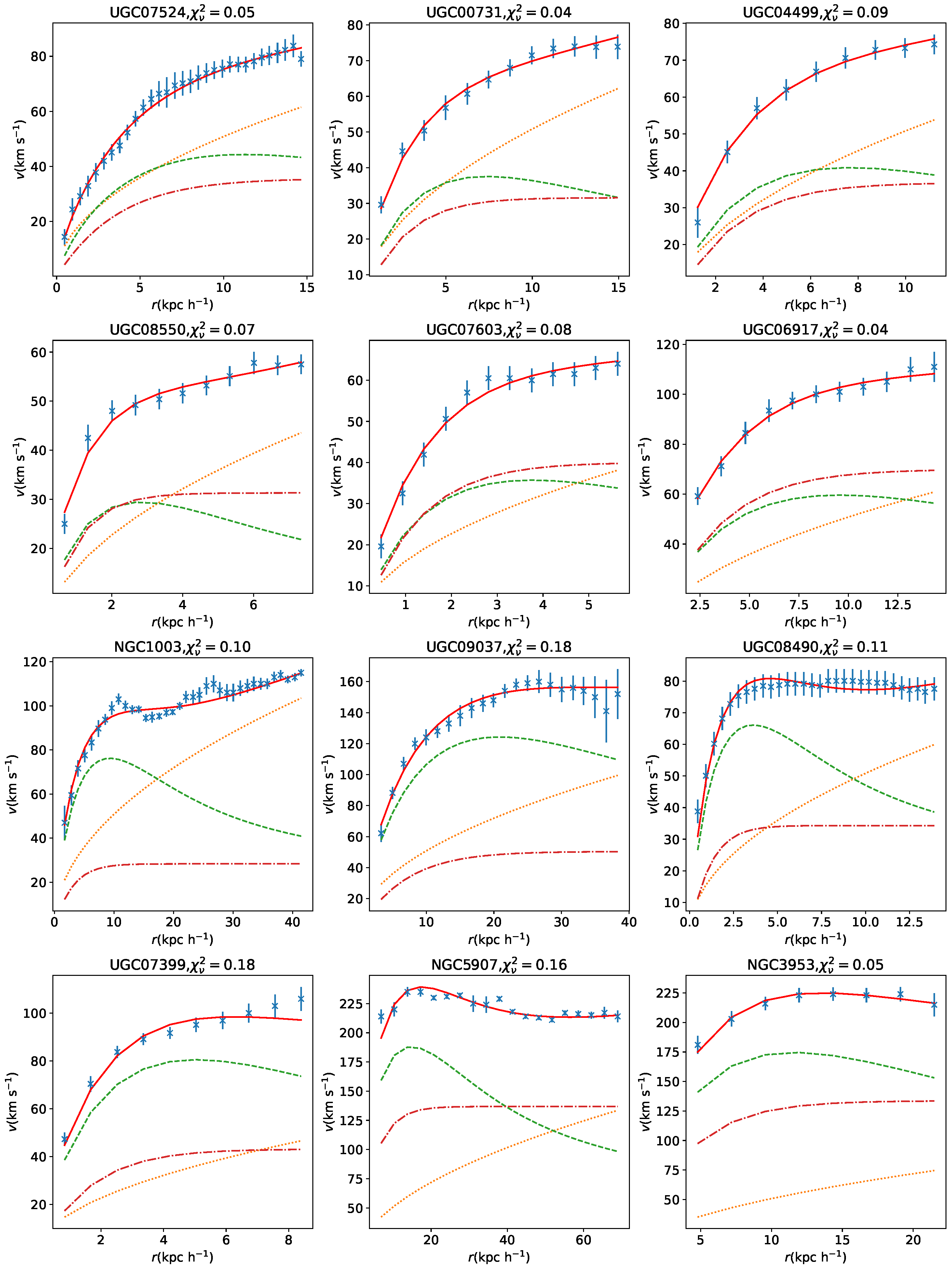
Disclaimer/Publisher’s Note: The statements, opinions and data contained in all publications are solely those of the individual author(s) and contributor(s) and not of MDPI and/or the editor(s). MDPI and/or the editor(s) disclaim responsibility for any injury to people or property resulting from any ideas, methods, instructions or products referred to in the content. |
© 2024 by the authors. Licensee MDPI, Basel, Switzerland. This article is an open access article distributed under the terms and conditions of the Creative Commons Attribution (CC BY) license (https://creativecommons.org/licenses/by/4.0/).
Copyright: This open access article is published under a Creative Commons CC BY 4.0 license, which permit the free download, distribution, and reuse, provided that the author and preprint are cited in any reuse.


