
Submitted:
11 July 2024
Posted:
12 July 2024
You are already at the latest version
Abstract
The study focuses on the free vibration analysis of beams made of axially functionally graded materials (AFGM) with curvilinear variable cross-sections along their length. The beams encompass various shapes, including concave and convex conic sections, with axial material properties varying according to polynomial and exponential laws. The equations of motion are derived using Hamilton's principle within the framework of Timoshenko beam theory. These governing equations, subjected to various boundary conditions, are solved using the differential transform method (DTM). The proposed solution technique is validated by comparing computed natural frequencies with existing in literature results and those obtained through three-dimensional finite element analysis in ABAQUS. The incorporation of material gradients into the beam finite element models was achieved through the user-defined material subroutine (UMAT). Additionally, a comprehensive study is conducted to examine the influence of various factors on the natural frequencies of functionally graded beams. These factors include parameters of material laws, types of variable beam shapes, slenderness ratio, and specific boundary conditions. This study provides a thorough understanding of the modal dynamics of the considered beams, offering valuable insights into the behavior of FGM structures.
Keywords:
free vibrations
; axially functionally graded material
; curvilinear tapered beam
; differential transform method
; ABAQUS
1. Introduction
Incorporating variable cross-sections in structural elements facilitates achieving an optimal balance between weight and strength, especially in critical applications like helicopter blades, airplane propellers, turbine blades, and wind turbines. Given their significance, there has been extensive research on the vibrations of these structures, often modeled as beams with variable cross-sections [1,2,3].
The increasing use of functionally graded materials (FGMs) in beam-like structures underscores the need to account for material variations. FGMs enhance performance and provide a continuous stress distribution, unlike the discontinuities found in laminated and sandwich composites [4,5,6].
While initial research focused on material gradients in the thickness direction, there is significant interest in longitudinally graded materials, known as axially functionally graded material (AFGM) structures. Analyzing the free vibration of non-uniform AFGM beams involves recognizing that the coefficients in the equations of motion, derived from any beam theory, vary with changes in cross-sections and material properties along the beam's length. Consequently, solving these differential equations is not straightforward and often necessitates numerical procedures.
In the context of one-dimensional continuous models with inhomogeneous material parameters, Elishakoff and co-workers have presented exact solutions for the fundamental frequency of diverse AFG beams with different end supports [7]. Yuan et al. (2016) [8] applied the confluent hypergeometric function method to obtain exact solutions for Timoshenko beams with varying bending stiffness. Zhao et al. (2017) [9] employed the Chebyshev polynomials theory to analyze the free vibration of both AFGM Euler–Bernoulli and Timoshenko beams with non-uniform cross-sections. Xie et al. (2017) [10] exploited the spectral collocation method to examine the statics and free vibrations of Euler–Bernoulli beams with axially variable cross-sections and material parameters, while Chen (2021) [11] extended this technique to non-uniform AFG Timoshenko beams. Additionally, Zhang et al. (2019) [12] utilized a Jacobi polynomial-based approximation, and Cao et al. (2019) [13] used the asymptotic perturbation method for vibrational analysis of non-uniform AFGM beams.
Other researchers have creatively adapted methods known from studying homogeneous beams with variable cross-sections to address solutions for non-uniform AFGM beams. For instance, Ghazaryan et al. (2018) [14] employed the differential transform method to study the free vibration characteristics of AFGM Euler-Bernoulli beams, while Rajasekaran and Tochaei (2014) [15] used both the differential transform element and differential quadrature element methods to study AFGM Timoshenko beams, both with varying cross-sectional profiles and material properties along the beam axis. Keshmiri et al. (2018) [16] determined natural frequencies of cantilever beams with different variable cross-sections and material gradients using the Adomian decomposition method (ADM), and Lin et al. (2022) [17] investigated the vibration of rotating non-uniform AFG Euler–Bernoulli beams using the Laplace ADM. In turn, Wang et al. (2022) [18] combined ADM with an iterative process for reliability analysis of composite beams with varying cross-section rigidities and mass distributions along their length. Mahmoud (2019) [19] presented a general solution for the free transverse vibration of cantilever non-uniform AFGM Euler-Bernoulli beams, loaded at the tips with point masses, using the Myklestad method. Chen et al. (2021) [20] employed the variational iteration method to determine the modal characteristics of tapered AFGM Euler–Bernoulli and Timoshenko beams. Liu et al. (2022) [21] proposed a closed-form dynamic stiffness formulation for free vibration analysis of tapered and/or FGM Euler–Bernoulli beams. Adelkhani and Ghanbari (2022) [22] analyzed the vibrations of tapered AFGM beams with nonlinear profiles using the point collocation method.
To investigate the dynamics of AFGM tapered beams under large deflection scenarios, Kumar et al. (2015) [23] employed the Rayleigh-Ritz method with start functions derived from nonlinear static analysis within the Euler-Bernoulli beam theory with von Kármán geometric nonlinearity, while Ghayesh (2018) [24] utilized the Galerkin method and the third-order shear deformation beam theory. Soltani and Asgarian (2019) [25] developed a hybrid approach combining the power series expansions and the Rayleigh-Ritz method for stability and free vibration analyses of non-uniform AFGM beams resting on Winkler-Pasternak elastic foundation. Singh and Sharma (2022) [26] carried out a vibration analysis of an AFGM non-prismatic Timoshenko beam under axial thermal variation in a humid environment using the harmonic differential quadrature method.
Finite element method-based approaches, tailored for precise and efficient study of this task, have also been proposed. Özdemir (2022) [27] studied free vibration and buckling characteristics of AFGM tapered rotating Euler–Bernoulli and Timoshenko beams with different end conditions using a two-noded beam element. Bazoune (2024) [28] proposed a Fourier-p element model for accurate predictions of Timoshenko-Ehrenfest beam frequencies with high precision compared to other existing models. Chen et al. (2019) [29] presented isogeometric analysis (IGA) in conjunction with elasticity theory for the three-dimensional vibration problem of AFGM beams with variable thickness. Murillo et al. [30] used the seven-parameter spectral finite element formulation to perform the analysis of FG shells of either uniform or non-uniform thickness. Burlayenko et al. (2024) [31] conducted simulations on the free vibrations of AFGM beams with non-uniform cross-sections, utilizing both one-dimensional and three-dimensional AFG finite element models developed in ABAQUS via user-defined subroutines [32,33,34].
Most of the examined non-uniform beams had rectangular cross-sections with linear taper. There were also studies on beams with parabolic and exponential thickness and constant or linear varying width, but less common. In some cases, vibrations of beams were investigated in scenarios such as truncated beams, beams with one sharp end, and beams with both ends sharp, as discussed in [1,3]. However, research on AFGM beams having arbitrary cross-section variations remains limited. Recently, Lee and Lee (2022) [35] studied the coupled flexural-torsional free vibration of circular horizontally curved beams with rectangular and elliptical cross-sections made of AFGMs with quadratic functions of Young’s modulus and the mass density, using the trial eigenvalue method and numerical integration within the Timoshenko and Saint-Venant beam theories. Rezaiee-Pajand et al. (2022) [36] proposed a closed-form solution for the lateral-torsional buckling moment of a bidirectional exponentially functionally graded monosymmetric C-shaped Euler–Bernoulli beam. Liu et al. (2024) [37] presented a nonlinear model to obtain the mode shape and frequency of FGM Euler-Bernoulli thin-walled beams with varying cross-sections, employing the perturbation approach and the Galerkin method. Other researchers have explored the concept of transforming the equations of motion of non-uniform FGM beams into those of equivalent uniform beams. For instance, Chen et al. (2017) [38] applied this idea to a specific class of non-uniform FGM beams. Additionally, Martin and Salehian (2020) [39] developed a method based on metric minimization, modal participation factor and the proper orthogonal decomposition to accurately approximate a Euler-Bernoulli motion equation with spatially varying coefficients with an equivalent constant coefficient model.
The literature search indicates that studying the dynamics of tapered AFGM beams involves complexities. While various techniques have been reported, closed-form solutions are limited to specific cross-sections, material variations and defined boundary conditions. Numerical methods like FEM are proficient but make it challenging to derive general conclusions about system behavior [40]. In this respect, accurate semi-analytical approaches can be a good alternative. Despite extensive research, the vibration characteristics of AFGM beams with arbitrary continuously variable cross-sections are not fully addressed. This study aims to use the differential transform method (DTM) to obtain accurate semi-analytical solutions for the free vibration of curvilinearly tapered AFGM beams under various boundary conditions, determining the effects of variable cross-sections on natural frequencies and mode shapes. This is an innovation of the present contribution.
2. AFGM Beams with Variable Cross-Section
2.1. Geometry of the Beams
Focusing on the closed-form solution of the free vibration problem, we aim to describe various non-uniform beam geometries in a unified analytical manner. One effective way to achieve this is by using rational Bézier curves [41].
We consider planar beams of length of that are symmetrical about their midlines, with the left ends positioned at the origin of the Cartesian coordinate system as shown in Figure 1. The top curve of these beams is a conic arc, represented by an algebraic quadratic equation in as follows:
The coefficients of (1) can be derived from the quadratic rational Bézier curve, which involves the control points , , and the weight , by utilizing the Gröbner basis as presented in [42]:
For convenience, let and denote the length of lines and , respectively, where is the shoulder point, is the midpoint of line and is a shape parameter related to . By specifying the coordinates of the points , , and the parameter , the implicit equation of a conic curve (1) can be constructed. The curve will have a convex upward shape if the vertex is above the line , and a concave downward shape if below the line as illustrated in Figure 1a and b, respectively.
2.2. Graded Materials of the Beams
We suppose that the materials of the beams with variable thickness are homogeneous in the thickness direction but graded along the axial direction. Consequently, the material properties, such as mass density and Young’s modulus, vary with the position along the -axis. Specifically, we analyze the following types of material distributions:
Type 1. The effective mass density and Young’s modulus are power-law functions of written as
where and are the mass density and Young’s modulus at , respectively; and are power coefficients that account for arbitrary variations of the material parameters along the beam’s length; and constant coefficients.
Type 2. The effective density and Young’s modulus follow exponential law functions of , given by
where the exponential function is determined by the parameter and gradation index , [29].
Type 3. The beams with variable thickness are composed of a metal-ceramic mixture. The effective material properties are calculated based on the rule of mixtures in the form:
where the subscripts ‘’ and ‘’ refer to the properties of metal and ceramic constituents, respectively; denotes the ceramic volume fraction, expressed as with the parameter and gradation index , [29].
Poisson’s ratio, is assumed to be constant throughout this study.
2.3. Governing Equations of the Beams
We consider the transverse vibrations of an AFGM beam in the -plane using the Timoshenko beam theory. The equations of motion governing such beams with generally variable cross-sections, in terms of the transverse displacement of the midline and the cross-sectional rotation angle at time are written as follows:
The rigidities and the inertia coefficients are expressed as integrals over the cross-sectional domain in the form:
where is the mass density, is the shear modulus and is the shear correction factor. Throughout this study, the shear factor is accepted as 5/6 unless specified otherwise.
Assuming simple harmonic oscillations, the deflection and the rotation angle can be expressed as
where and are the amplitudes of the displacement and rotation angle, respectively, is the angular frequency; and represents the imaginary unit.
Substituting (7) into (5) yields a system of coupled ordinary differential equations that describe the free transverse vibrations of a Timoshenko beam with a non-uniform cross-section as
Herewith, the rigidities and inertia coefficients (6) can be conveniently presented by the expressions:
where and are the area and second inertia moment of the cross-section, respectively.
3. Solution Methodology
3.1. Differential Transform Method
Due to the variable coefficients, reflecting the dependence of material properties and cross-sectional geometry on the -coordinate, the coupled nature of the differential equations in (8) presents mathematical challenges for finding a closed-form solution. To address this, we employ the differential transform method (DTM) for its versatility and simplicity. This method converts the differential equations into a set of recurrent algebraic equations, enabling the solution to be represented as an infinite power series. The fundamental aspects of the DTM can be found in G.E. Pukhov’s original publications [43].
We reformulate system (8) a more suitable form for applying the DTM as follows:
where the variable coefficients are defined as , , , , . Here, and in what follows, the prime denotes differentiation with respect to the -coordinate.
Hence, the solution of (10) at a specific point within the interval in the domain of differential transformation is expressed by the recurrent algebraic equations:
where , is a unity image, and , , , , , , and are the images of the unknown amplitudes and and the corresponding functional coefficients in (10), respectively.
By incrementing the index sequentially, we can generate all images from (11) except for , , , and . Consequently, the system (11) can be simplified to the form:
where the explicit forms of the recurrent coefficients in (12) are presented in [44] (see Appendix B).
Given that the images and at depend on , , and , the original functions and can be reconstructed for a selected number of images as follows:
Taking into account the actual boundary conditions applied to the beam ends, which involve the transverse displacement , rotation angle , bending moment , and shear force , such that
we can formulate the eigenvalue problem for each case of constraints in the form:
Here, the functions are appropriate polynomials of the unknown angular frequency , which involve the recurrent coefficients and the power terms of .
Finally, the eigenvalues are computed by solving the root-finding problem resulting from the equation:
A computational program has been developed in the Matlab environment to apply the DTM for analyzing the free vibration of curvilinear tapered inhomogeneous Timoshenko beams. The eigenvalue problem is addressed using standard algorithms provided in the Matlab package [45].
3.2. Finite Element Modeling
To ensure the accuracy and validation of the proposed semi-analytical methodology for analyzing the free vibration parameters of curvilinearly tapered AFGM beams, a finite element model has been developed and utilized for comparison purposes. It is well-known that the optimal modeling strategy involves using graded finite elements (GFEs), which allow for the variation of material properties at the element level. Additionally, advanced three-dimensional models are essential to precisely capture the non-uniform geometry of axially inhomogeneous beams [31].
The free vibration analysis of AFGM beams is conducted using ABAQUS [46], incorporating a user-defined material subroutine (UMAT) to implement material gradients into a convenient three-dimensional element, C3D20, as detailed in [31,33] and illustrated in Figure 2b. The material gradient is assigned within the element volume during the computation of the element stiffness matrix, using Gauss quadrature, as follows:
where the indices , , and refer to the integration points over the element volume, is the determinant of the geometric Jacobian matrix, , , and are the Gaussian weights; stands for a matrix of gradients of the shape functions for the 3-D element and the material matrix of the 3-D GFE relevant to this study can be found in [33].
ABAQUS currently does not support calculating the mass matrix based on a user-defined mass density in frequency analysis [46]. The elements available in ABAQUS use a constant mass density, i.e.
where is an element interpolation matrix.
To address this limitation, we assigned a constant effective mass density within the GFE by using an average value of the actual mass density distribution over the beam's volume in the form:
In the case of the free vibration analysis without damping, the global discrete system of governing equations of motion is reduced to the problem of eigenvalues and associated eigenvectors, which is written as follows
where , are global mass and stiffness matrices, obtained by assembling the formulated element mass and stiffness matrices; is the undamped circular frequency, is the vector of nodal displacements associated with oscillations at each . The free vibration analysis is carried out using linear perturbation load step, obtaining the eigenvalues by means of Lanczos or subspace iteration methods [46]. Figure 2a illustrates a 3-D finite element beam model created using the ABAQUS pre-processor, utilizing the 'loft' feature. To provide accurate results, the element aspect ratio in the mesh was consistently maintained close to one throughout all subsequent calculations.
4. Results
We will now examine beams with various curvilinear tapers in rectangular cross-sections, incorporating three distinct material variations along the beam axis. This analysis aims to demonstrate the effectiveness of the proposed computational technique by comparing the results with those obtained from other methods. First, we validate the accuracy of the DTM approach by benchmarking our findings against known solutions for uniform homogeneous and inhomogeneous Timoshenko beams under various boundary conditions. Then, we present a selection of examples for curvilinear taper beams, including both known and previously unexplored cases, to further illustrate the method's applicability and provide new insights that may be valuable to other researchers in this field.
4.1. Homogeneous Timoshenko Beams with Uniform Cross-Sections
The accuracy and effectiveness of the proposed approach are first benchmarked by computing the frequencies of homogeneous beams with uniform cross-sections.
We consider geometrically uniform () homogeneous ( with unit coefficients in (2) ) beams with clamped-clamped (C-C), clamped-free (C-F), and simply supported (S-S) boundary conditions. The material and geometric parameters of the beams are listed in Table 1.
The first seven natural frequencies of the S-S, C-C, and C-F beams compared with those computed using the dynamic stiffness matrix method (DSM) in conjunction with the Timoshenko beam theory in [47] are presented in Table 2.
As shown in Table 2, there is excellent agreement between the solutions obtained using the DTM and DSM methods for all vibrational modes.
4.2. Inhomogeneous Timoshenko beams with uniform cross-sections
Next, the ability of the proposed approach to accurately predict the frequencies of beams with uniform cross-sections made of inhomogeneous materials is evaluated.
We assume that the beam’s mass density and modulus of elasticity follow power-law distributions of Type 1 as described in (2). Since natural frequencies for Timoshenko beams under these conditions are not documented in the literature, we will compare our results with those obtained using the Euler-Bernoulli beam theory in [14] for AFGM beams with a slenderness ratio of . The geometrical and material parameters are consistent with those detailed in [14] (see Tables 4–6 and Appendix B).
The comparison of the first five dimensionless frequencies for the cantilever AFGM beam is presented in Table 3. Furthermore, to extend this study to beams, where shear deformation plays a significant role, we also provide in Table 3 the natural frequencies computed for beams with a slenderness ratio of 10.
Upon reviewing Table 3, it becomes evident that both Euler-Bernoulli and Timoshenko beams with slenderness ratio of 50 demonstrate excellent agreement for the fundamental frequency and show slight deviations for higher frequencies. This is because the Euler-Bernoulli beam theory overestimates especially higher frequencies due to its neglect of shear effect. Specifically, when the slenderness ratio is 10, the fundamental frequencies of the beams show only satisfactory matching, while significant discrepancies are observed in higher-order frequencies, consistent with theoretical expectations.
In the second example, we evaluate the accuracy of predicted natural frequencies for exponential AFGM beams. The current results are compared with those obtained in [11] using the Chebyshev collocation method. The beams are composed of zirconia and aluminum with axial gradation according to law (4), where the ceramic volume fraction is an exponential function: . The material and geometrical properties of the beams are described in [11] and detailed in Table 4 as follows:
The computed first four dimensionless natural frequencies of the exponential-law AFGM beams under S-S and C-C boundary conditions for various exponents compared with the results in [11] are given in Table 5.
From Table 5, it is obvious that the present results for all first four frequencies closely align with those obtained in the referenced study.
Finally, uniform aluminum-zirconia Timoshenko beams with axial variation of the material characteristics according to the power-law function of the ceramic volume fraction in the rule of mixtures (4) are tested. The natural frequencies of these beams are benchmarked against the findings in [15]. The parameters of the AFGM beams are the same as those in [15] and are listed in Table 4.
The first four dimensionless natural frequencies of the AFGM beams under C-F, S-S and C-C boundary conditions for various indices , compared with the solutions obtained using the differential quadrature element method in [15], are shown in Table 6.
Inspecting Table 6 reveals excellent agreement between the first four frequencies obtained in this study and those reported in the referenced research across all boundary conditions and power indices.
It should be noted that throughout this series of examples, the proposed approach demonstrates high accuracy, efficiency, and rapid convergence. Only thirty terms in the series expansions (13) are sufficient to yield accurate results for the first several natural frequencies.
4.3. Homogeneous Timoshenko Beams with Curvilinearly Tapered Cross-Sections
In order to demonstrate the applicability and effectiveness of the DTM in solving the free vibration problem for axially curvilinear cross-sectional beams, we now consider various specific cases. Whenever possible, we compare the results obtained using DTM with those already documented in the literature. In cases, where comparative data is not available, we perform the frequency analysis using ABAQUS software.
The first problem addressed is a homogeneous beam with a double-parabolic taper, truncated at the left end. The shape of the parabolic taper beam is analytically defined by the weight , the parameter equals to the truncation factor and the tringle specified as shown in Figure 3a.
Due to the lack of data for such Timoshenko beams in the published literature, the results are compared with those obtained using the Rayleigh-Ritz method within the Euler-Bernoulli beam theory in [2]. Table 7 presents the first three dimensionless frequencies for both the reference Euler-Bernoulli and present Timoshenko beams with a slenderness ratio under three different boundary conditions and different truncation factors.
One can observe from Table 7 that the eigenfrequencies closely match for both types of beams when the truncation factor is small. However, as the truncation factor increases, discrepancies between them become more pronounced, especially for the third mode. This difference is anticipated because shorter beams necessitate accounting for shear deformation, which the simpler Euler-Bernoulli beam model does not address.
The second benchmark example involves a beam with a parabolic-tapered height and constant width, truncated at the left end and tapered to a point at the right end (), as illustrated in Figure 3b. A detailed specification of this beam configuration is provided in [3]. The analytical presentation of this shape of the parabolic beam with Bézier curves is discussed in Section 2.1.
Once again, due to limited availability of data for Timoshenko beams in the existing literature, comparisons are made with results obtained using hypergeometric functions within the framework of the Euler-Bernoulli beam theory, as described in [3]. Table 8 displays the first four dimensionless frequencies of cantilever Euler-Bernoulli and Timoshenko beams with a slenderness ratio for various truncation factors.
From Table 8, one can see that the compared natural frequencies exhibit close agreement. Similar to the previous example, as the beam length decreases, discrepancies between the present and benchmarked results increase, especially for higher modes, due to the greater influence of shear deformation, as discussed earlier.
Therefore, these examples thoroughly confirm the reliability of the proposed computational method for analyzing curvilinear tapered beams.
4.4. AFGM Timoshenko Beams with Curvilinearly Tapered Cross-Sections
This subsection presents the performance of the DTM for frequency analysis of inhomogeneous curvilinearly tapered beams of convex-up and concave-down shapes, referred to as plump and slender models in [29], illustrated in Figure 1a,b, respectively. The material properties of the beams vary axially according to the laws specified in (3) for Type 2 and (4) for Type 3 distributions. Detailed geometric and material properties of the beams can be found in [29] and are summarized in Table 9.
First, we analyze beams with varying thickness and constant width for both Type 2 and Type 3 material laws. The exponential law (3) with parameter and gradient indices is applied to beams made of aluminum, whereas the power-law (4) with parameter and gradient indices is utilized for beams composed of a combination of steel (SUS304) and ceramic (Si3N4) phases, as done in [29].
Table 10 presents the first two frequencies associated with the bending modes of the curvilinear taper beams with C-C boundary conditions. These frequencies are compared with those computed using NURBS in the 3-D finite element analysis conducted in [29].
The current results align satisfactory with the reference data, demonstrating differences of less than 0.6% for the fundamental frequency and less than 9% for the second frequency in the plump beams. For slender beams, the discrepancies are approximately 3% for both frequencies. These deviations arise from differences in modeling approaches. The current model uses a line beam structure with a first-order shear theory, whereas the IGA analysis in [29] employs a more detailed 3-D beam modeling approach.
Next, we analyze the parabolic convex beams depicted in Figure 3b. These beams feature a parabolic taper in height and maintain a constant width. They are truncated at the left end with a fixed factor , while the right end is characterized by a variable truncation factor . The beam ends are subjected to C-C and C-F constraints. The material constants, given in Table 1, vary along the beam length according to the Type 1 material law with a linear distribution for Young's modulus () and a parabolic distribution for mass density () as described in (2). Detailed specifications of these beam configurations are provided in [23].
While benchmark results for the fundamental frequencies of these beams are available in [23], higher-order frequencies are absent in the existing literature. Therefore, the results obtained using the DTM are validated against finite element analysis for these beams, as discussed in Section 3.2.
The comparison of first five dimensionless bending frequencies , depending on the truncation factor for the two types of boundary conditions is shown in Table 11. It is observed that the differences between dimensionless fundamental frequencies obtained from the present analysis, published results and FEM predictions are quite small. However, the higher frequencies show more significant deviations between the DTM and FEM solutions. Likely, these discrepancies between the two sets of data are attributed to methodological differences in formulation and solution approach. Overall, these findings confirm the reliability of the DTM approach within acceptable limits.
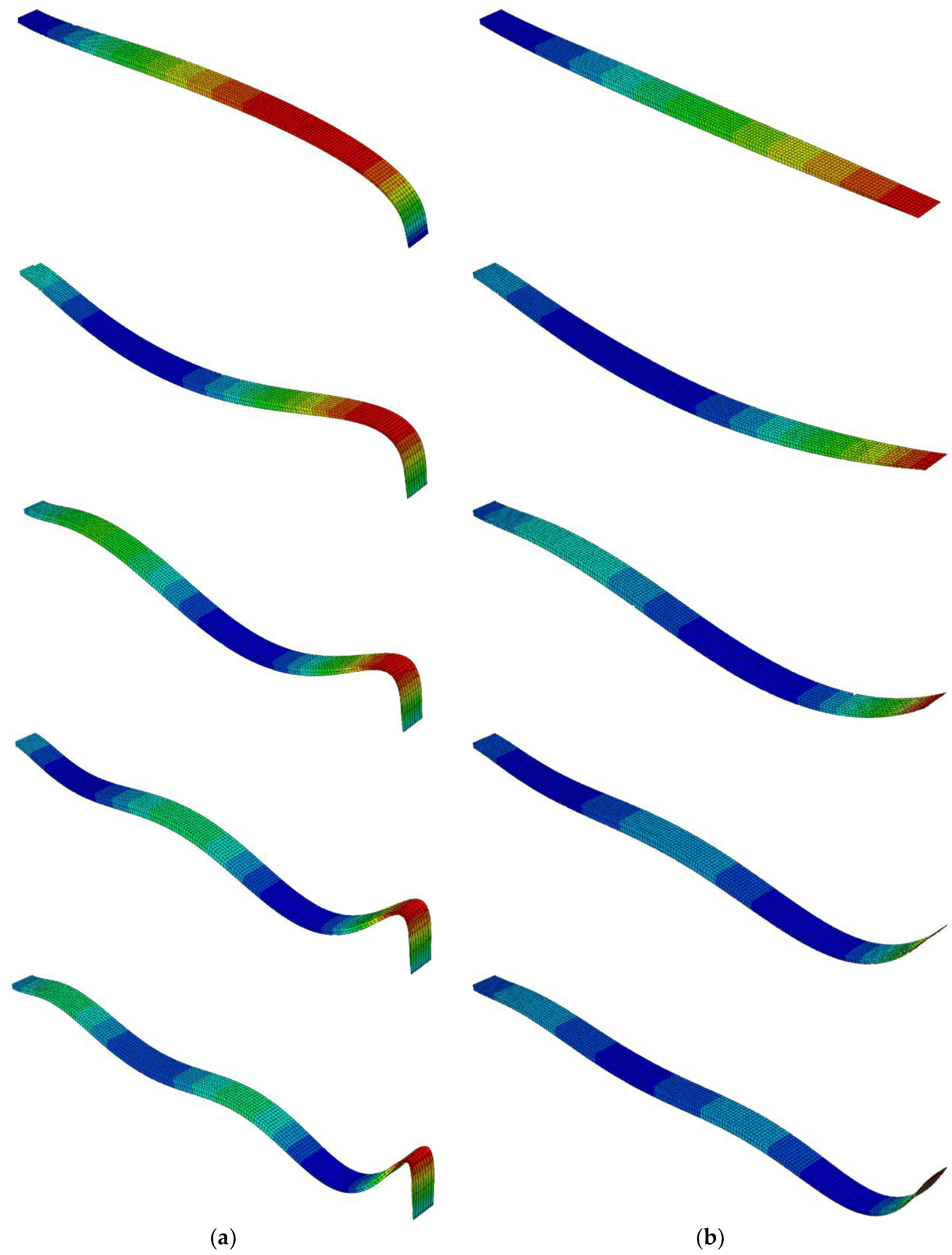
As mode shapes play a crucial role in evaluating the accuracy of structural dynamics modeling, the first five bending mode shapes associated with the appropriate frequencies of AFGM beams with for C-C and C-F boundary conditions, as listed in Table 11 and obtained using the DTM, are plotted in Figure 4a,b, respectively.
Analogously, Figure 5a,b illustrate the bending mode shapes of the same truncated AFGM beams, constructed based on the FEM results, which are given in Table 11.
It is worth noticing that the geometric non-uniformity and the variation of material parameters along the beam length significantly affect the mode shapes. The figures clearly show that the positions of the nodal points shift along the beam length, and this shift is more pronounced as the truncation factor becomes smaller.
4.5. AFGM Timoshenko Beams with Curvilinearly Double-Tapered Cross-Sections
To the best of authors' knowledge, benchmark results for curvilinearly double-tapered AFGM beams are not available in the existing literature. Hence, the results of the present analysis are validated against axial plumb and slender beams with Type 2 and Type 3 material distributions, as considered in [29], which feature variable thickness and constant width. Further, the analysis will be etended to include beams with double-tapered cross-sectional variations. The geometrical and material parameters are identical to those used in the previous examples of curvilinear taper beams with exponential and power-law gradations as presented in [29].
Figure 5.
Mode shapes of truncated AFGM beams with parabolic taper height and constant width obtained from 3- D FEM analysis: (a) C-C boundary conditions; (b) C-F boundary conditions.
Figure 5.
Mode shapes of truncated AFGM beams with parabolic taper height and constant width obtained from 3- D FEM analysis: (a) C-C boundary conditions; (b) C-F boundary conditions.
The first two dimensionless frequencies of axially graded Type 2 plump and slender C-C beams with variable thickness and constant width, as well beams with simultaneously variable thickness and width, depending on the exponential law parameter and gradient index are collected in Table 12. Satisfactory agreement between the reference and present results for plump and slender AFGM beams with variable thickness is observed. The errors between the frequencies fall within the range observed for frequencies of similar beams with and in Table 10. In particular, minor deviations are noted for the first frequency, while higher discrepancies are observed for the second frequency.
Upon reviewing Table 12, it becomes evident that introducing variations in width influences the frequencies of the beams. Specifically, plump double-tapered beams show slightly lower frequencies compared to those with only variable thickness, whereas slender double-tapered beams exhibit a slight increase. However, the trends in frequency changes with increasing gradient index and parameter remain consistent for both beams with only variable thickness and double-tapered beams. The frequencies increase with higher and . This increase is more pronounced as or become larger.
Analogously, axially graded Type 3 plump and slender C-C beams with variable thickness and constant width, and with simultaneously variable thickness and width are examined. Table 13 presents the first two dimensionless frequencies of these beams for different values of power law parameter and gradient index .
It is found in Table 13 that the agreement between the results obtained from the IGA analysis in [29] and the present study is satisfactory, with errors comparable to those observed for Type 3 plump and slender C-C beams with and in Table 11. Additionally, Table 13 shows that introducing variable width along with variable height has similar effects on the frequencies of both beams with variable thickness only and curvilinearly double-tapered beams, similar to what was observed for Type 2 plump and slender C-C beams, as mentioned earlier.
On the other hand, the trends of the frequency changes with increasing and are found to be opposite to those in Type 2 plump and slender C-C beams. In Type 3 plump and slender beams, the frequencies decrease with higher values of and . This decrease begins more rapidly and exhibits a faster decay as or increase.
Table 14 presents the dimensionless natural frequencies of beams with variable thickness only and curvilinearly double-tapered beams under different boundary conditions. The calculation errors for the first and second frequencies are within 3%. Notably, the second bending frequency is not available from the IGA analysis in [29] in some cases. Analyzing the data in Table 14, it is evident that the frequencies of curvilinearly double-tapered beams behave similarly to those of beams with variable thickness only, depending on the boundary conditions. In particular, the highest frequencies correspond to C-C restraints, while the lowest frequencies are observed under C-F boundary conditions.
5. Conclusions
Free vibration analysis of axially functionally graded beams with curvilinear taper cross-sections and various material distributions is performed using the semi-analytical approach of the differential transform method. Unlike standard procedure that impose boundary conditions on transformed images of unknown functions, the present DTM approach integrates various boundary conditions directly into the original continuous problem formulation. The non-uniform beam shapes, defined as conic sections, are analytically described using rational Bézier curves in the Gröbner basis in a unified manner.
The equations of motion for free vibration are derived by principle of virtual work under the assumptions of the Timoshenko beam theory. It is assumed that both the material properties of the beam and its geometric features vary continuously along the axial direction.
Comparisons are presented to validate the accuracy and assess the efficiency of the proposed computational technique. The computed examples encompass both well-documented cases and previously unexamined scenarios, ranging from uniform homogeneous and inhomogeneous beams to curvilinearly double-tapered axially functionally graded beams. In the cases, where benchmark results are unavailable in the literature, the current DTM solutions are compared with our own FEM simulations. The three-dimensional finite element modeling was conducted using the ABAQUS code with a user-defined subroutine (UMAT) to incorporate material gradients into the 3-D element C3D20.
Based on these results, the DTM in its proposed formulation exhibits excellent performance in modeling the free vibration of beams with complex geometry and material distribution. This study provides new results from frequency analysis of curvilinearly double-tapered AFGM beams. It was found that introducing simultaneous variations in height and width of the beam cross-section influences the beam’s frequencies. While these changes may not be substantial, conducting accurate dynamic structural modeling remains crucial. Therefore, these findings can be useful in the design process of axially functionally graded beams and serve as benchmarks for researchers interested in exploring similar problems using alternative methods.
Author Contributions
Conceptualization, V.N.B. and R.K.; methodology, V.N.B.; software, V.N.B.; validation, V.N.B. and S.D.D.; writing—original draft preparation, V.N.B, R.K. and S.D.D.; writing—review and editing, V.N.B. and R.K. All authors have read and agreed to the published version of the manuscript.
Funding
This research received no external funding
Data Availability Statement
The raw data supporting the conclusions of this article will be made available by the authors on request.
Acknowledgments
The first author acknowledges that his research was conducted in compliance with the project of the Ministry of Education and Science of Ukraine, under grant agreement no. 0124U000975.
Conflicts of Interest
The authors declare no conflicts of interest.
References
- Ece, M. C.; Aydogdu, M.; Taskin, V. Vibration of a variable cross-section beam. Mech. Res. Commun. 2007, 34, 78–84. [Google Scholar] [CrossRef]
- Zhou, D.; Cheung, Y.K. The free vibration of a type of tapered beams. Comput. Methods Appl. Mech. Engrg. 2000, 188, 203–216. [Google Scholar] [CrossRef]
- Caruntu, D.I. Dynamic modal characteristics of transverse vibrations of cantilevers of parabolic thickness. Mech. Res. Commun. 2009, 36, 391–404. [Google Scholar] [CrossRef]
- Burlayenko, V.N.; Sadowski, T. Dynamic analysis of debonded sandwich plates with flexible core – Numerical aspects and simulation. In Shell-like Structures; Altenbach, H.; Eremeyev, V., Eds.; Springer: Berlin, Heidelberg, 2011; Adv. Struct. Mater. Vol. 15, pp. 415–440.
- Burlayenko, V.N.; Altenbach, H.; Sadowski, T. Dynamic fracture analysis of sandwich composites with face sheet/core debond by the finite element method. In Dynamical Processes in Generalized Continua and Structures; Altenbach, H.; Belyaev, A.; Eremeyev, V.; et al., Eds.; Springer: Cham, 2019; Adv. Struct. Mater. Vol 103, pp. 163 – 194.
- Carrera, E.; Demirbas, M.D.; Augello, R. Evaluation of stress distribution of isotropic, composite, and FG beams with different geometries in nonlinear regime via Carrera-unified formulation and Lagrange polynomial expansions. Appl. Sci. 2021, 11, 10627. [Google Scholar] [CrossRef]
- Elishakoff, I. Eigenvalues of Inhomogenous Structures: Unusual Closed-form Solutions. CRC Press: New York, 2005.
- Yuan, J.; ·Pao, Y.-H.; ·Chen, W. Exact solutions for free vibrations of axially inhomogeneous Timoshenko beams with variable cross section. Acta. Mech. 2016, 227, 2625–2643. [Google Scholar] [CrossRef]
- Zhao, Y.; Huang, Y.; Guo, M. A novel approach for free vibration of axially functionally graded beams with non-uniform cross-section based on Chebyshev polynomials theory. Compos. Struct. 2017, 168, 277–284. [Google Scholar] [CrossRef]
- Xie, X.; Zheng, H.; Zou, X. An integrated spectral collocation approach for the static and free vibration analyses of axially functionally graded nonuniform beams. Proc. Inst. Mech. Eng., Part C 2017, 231(13), 2459–2471. [Google Scholar] [CrossRef]
- Chen, W.-R. Vibration analysis of axially functionally graded Timoshenko beams with non-uniform cross-section. Lat. Am. J. Solids Struct. 2021, 18(07), 1–18. [Google Scholar] [CrossRef]
- Zhang, X.F.; Zhuang, Y.; Zhou, Y.J.J. A Jacobi polynomial based approximation for free vibration analysis of axially functionally graded material beams. Comput. Struct. 2019, 225, 111070. [Google Scholar] [CrossRef]
- Cao, D.X.; Wang, J.J.; Gao, Y.H.; et al. Free vibration of variable width beam: asymptotic analysis with FEM simulation and experiment confirmation. J. Vib. Eng. Technol. 2019, 7, 235–240. [Google Scholar] [CrossRef]
- Ghazaryan, D.; Burlayenko, V.N.; Avetisyan, A.; Bhaskar, A. Free vibration analysis of functionally graded beams with non-uniform cross-section using the differential transform method. J. Eng. Math. 2018, 110, 97–121. [Google Scholar] [CrossRef]
- Rajasekaran, S.; Tochaei, E.N. Free vibration analysis of axially functionally graded tapered Timoshenko beams using differential transformation element method and differential quadrature element method of lowest-order. Meccanica 2014, 49, 995–1009. [Google Scholar] [CrossRef]
- Keshmiri, A.; Wu, N.; Wang, Q. Free vibration analysis of a nonlinearly tapered cone beam by Adomian decomposition method. Int. J. Struct. Stab. Dyn. 2018, 18(07), 1850101. [Google Scholar] [CrossRef]
- Lin, M.-X.; Deng, C.-Y.; Chen, C.-K. Free vibration analysis of non-uniform Bernoulli beam by using Laplace Adomian decomposition method. Proc. Inst. Mech. Eng., Part C 2022, 236(13), 7068–7078. [Google Scholar] [CrossRef]
- Wang, P.; Wu, N.; Sun, Z.; Luo, H. Vibration and reliability analysis of non-uniform composite beam under random load. Appl. Sci. 2022, 12, 2700. [Google Scholar] [CrossRef]
- Mahmoud, M. Natural frequency of axially functionally graded, tapered cantilever beams with tip masses. Eng. Struct. 2019, 187, 34–42. [Google Scholar] [CrossRef]
- Chen, Y.; Dong, S.; Zang, Z; et al. Free transverse vibrational analysis of axially functionally graded tapered beams via the variational iteration approach. J. Vib. Control 2021, 27(11-12), 1265–1280. [Google Scholar] [CrossRef]
- Liu, X.; Chang, L.; Banerjee, J.R.; Dan, H.-C. Closed-form dynamic stiffness formulation for exact modal analysis of tapered and functionally graded beams and their assemblies. Int. J. Mech. Sci. 2022, 214, 106887. [Google Scholar] [CrossRef]
- Adelkhani, R.; Ghanbari, J. Vibration analysis of nonlinear tapered functionally graded beams using point collocation method. Int. J. Comput. Methods Eng. Sci. 2022, 23(4), 334–348. [Google Scholar] [CrossRef]
- Kumar, S.; Mitra, A.; Roy, H. Geometrically nonlinear free vibration analysis of axially functionally graded taper beams. Eng. Sci. Technol. Int. J. 2015, 18, 579–593. [Google Scholar] [CrossRef]
- Ghayesh, M.H. Nonlinear vibration analysis of axially functionally graded shear-deformable tapered beams. Appl. Math. Model. 2018, 59, 583–596. [Google Scholar] [CrossRef]
- Soltani, M.; Asgarian, B. New hybrid approach for free vibration and stability analyses of axially functionally graded Euler-Bernoulli beams with variable cross-section resting on uniform Winkler-Pasternak foundation. Lat. Am. J. Solids Struct. 2019, 16(3), 1–25. [Google Scholar] [CrossRef]
- Singh, R.; Sharma, P. Vibration analysis of an axially functionally graded material non-prismatic beam under axial thermal variation in humid environment. J. Vib. Control 2022, 28(23-24), 3608–3621. [Google Scholar] [CrossRef]
- Özdemir, Ö. Vibration and buckling analyses of rotating axially functionally graded nonuniform beams. J. Vib. Eng. Technol. 2022, 10, 1381–1397. [Google Scholar] [CrossRef]
- Bazoune, A. Free vibration frequencies of a variable cross-section Timoshenko-Ehrenfest beam using Fourier-p element. Arab. J. Sci. Eng. 2024, 49, 2831–2851. [Google Scholar] [CrossRef]
- Chen, M.; Jin, G.; Zhang, Y.; Niu, F.; Liu, Z. Three-dimensional vibration analysis of beams with axial functionally graded materials and variable thickness. Compos. Struct. 2019, 207, 304–322. [Google Scholar] [CrossRef]
- Valencia Murillo, C.E.; Gutierrez Rivera, M.E.; Flores Samano, N.; Celaya Garcia, L.D. A seven-parameter spectral/hp finite element model for the linear vibration analysis of functionally graded shells with nonuniform thickness. Appl. Sci. 2023, 13, 11540. [Google Scholar] [CrossRef]
- Burlayenko, V.N.; Kouhia, R.; Dimitrova, S.D. One-dimensional vs. three-dimensional models in free vibration analysis of axially functionally graded beams with non-uniform cross-sections. Mech. Compos. Mater. 2024, 60, 83–102. [Google Scholar] [CrossRef]
- Burlayenko, V.N. Modelling thermal shock in functionally graded plates with finite element method. Adv. Mater. Sci. Eng. 2016, 2016, 7514638, 1-12. [Google Scholar] [CrossRef]
- Burlayenko, V.N.; Dimitrova, S.D.; Altenbach, H. A material model-based finite element free vibration analysis of one-, two- and three-dimensional axially FGM beams. Proceedings of Conference 2021 IEEE KhPI Week on Advanced Technology, Kharkiv, Ukraine, 13 – 17 September 2021; pp. 628–633. [Google Scholar]
- Burlayenko, V.N. A continuum shell element in layerwise models for free vibration analysis of FGM sandwich panels. Continuum Mech. Thermodyn. 2021, 33, 1385–1407. [Google Scholar] [CrossRef]
- Lee, J.K. , Lee, B.K. Coupled flexural-torsional free vibration of an axially functionally graded circular curved beam. Mech. Compos. Mater. 2022, 57, 833–846. [Google Scholar] [CrossRef]
- Rezaiee-Pajand, M. , Masoodi, A.R. & Alepaighambar, A. Lateral-torsional buckling of a bidirectional exponentially graded thin-walled C-shaped beam. Mech. Compos. Mater. 2022, 58, 53–68. [Google Scholar]
- Liu, P.; Tang, J.; Jiang, B.; Li, Y. Nonlinear parametric vibration analysis of the rotating thin-walled functionally graded material hyperbolic beams. Math. Meth. Appl. Sci. 2024, 47, 2952–2965. [Google Scholar] [CrossRef]
- Chen, W. R.; Chang, H. Closed-form solutions for free vibration frequencies of functionally graded Euler-Bernoulli beams. Mech. Compos. Mater. 2017, 53, 79–98. [Google Scholar] [CrossRef]
- Martin, B.; Salehian, A. Techniques for approximating a spatially varying Euler-Bernoulli model with a constant coefficient model. Appl. Math. Model. 2020, 79, 260–283. [Google Scholar] [CrossRef]
- Rao, S.S. Mechanical Vibrations, 4th ed.; Person Prentice Hall: New York, 2004. [Google Scholar]
- Piegl, L; Tiller, W. Conies and Circles. In The NURBS books, 2nd ed.; Springer-Verlag: Berlin Heidelberg, 1995; pp. 281–331. [Google Scholar]
- Anwar, Y. R.; Tasman, H.; Hariadi, N. Determining implicit equation of conic section from quadratic rational Bézier curve using Gröbner basis. J. Phys.: Conf. Ser. 2021, 2106, 012017. [Google Scholar] [CrossRef]
- Pukhov, G. E. Differential Transformations and Mathematical Modeling of Physical Processes; Naukova Dumka: Kiev, Ukraine, 1986. [Google Scholar]
- Burlayenko, V.N.; Altenbach, H.; Dimitrova, S.D. Modal characteristics of functionally graded porous Timoshenko beams with variable cross-sections. Compos.Struct. 2024, 342, 118273. [Google Scholar] [CrossRef]
- MATLAB version: 9.1.0 (R2016b), The MathWorks Inc., Natick, Massachusetts, United States, 2016. URL https://www.mathworks.com.
- ABAQUS User’s Manual, Version 2016. Dassault Systèmes Simulia Corp., Providence, RI, USA, 2016.
- Zhou, H.; Ling, M.; Yin, Y.; Hu, H.; Wu, S. Exact vibration solution for three versions of Timoshenko beam theory: A unified dynamic stiffness matrix method. J. Vib. Control. 2023, 1–15. [Google Scholar]
Figure 1.
The geometries of AFGM beams with variable thickness: (a) Convex upward shape; (b) Concave downward shape.
Figure 1.
The geometries of AFGM beams with variable thickness: (a) Convex upward shape; (b) Concave downward shape.
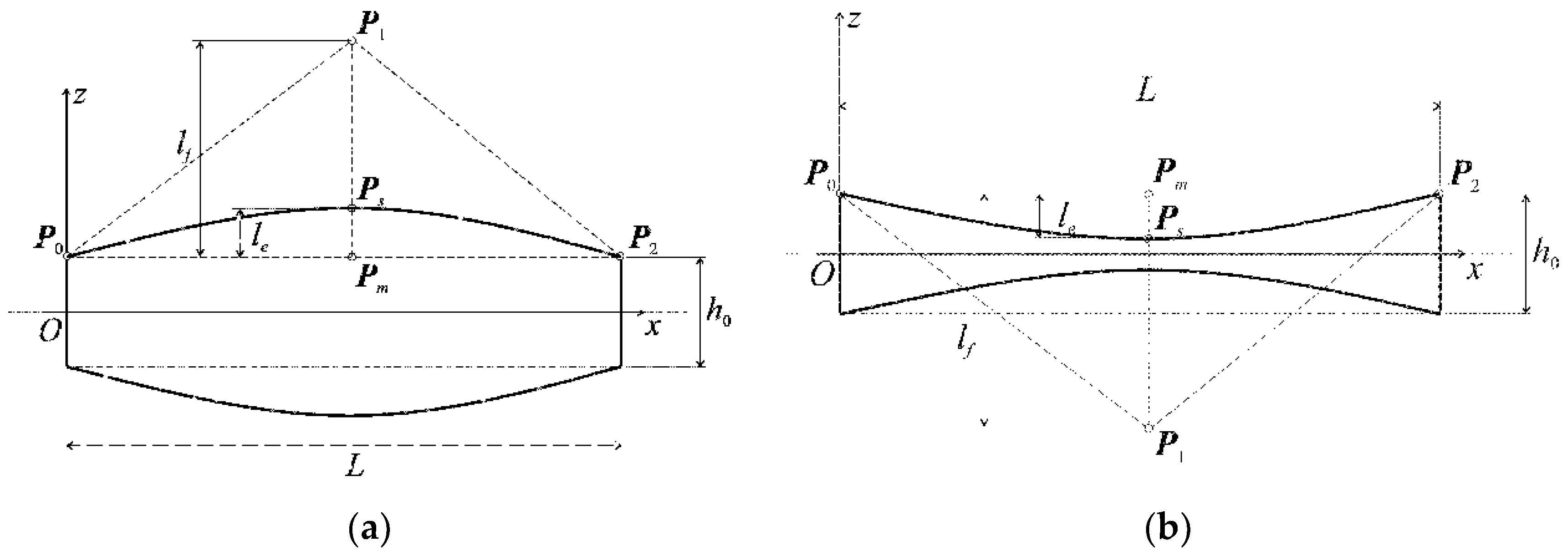
Figure 2.
Finite element model of the curvilinear tapered beam: (a) Finite element discretization with 3-D finite elements; (b) 20-node three-dimensional element C3D20 with a 3×3×3 point integration scheme.
Figure 2.
Finite element model of the curvilinear tapered beam: (a) Finite element discretization with 3-D finite elements; (b) 20-node three-dimensional element C3D20 with a 3×3×3 point integration scheme.
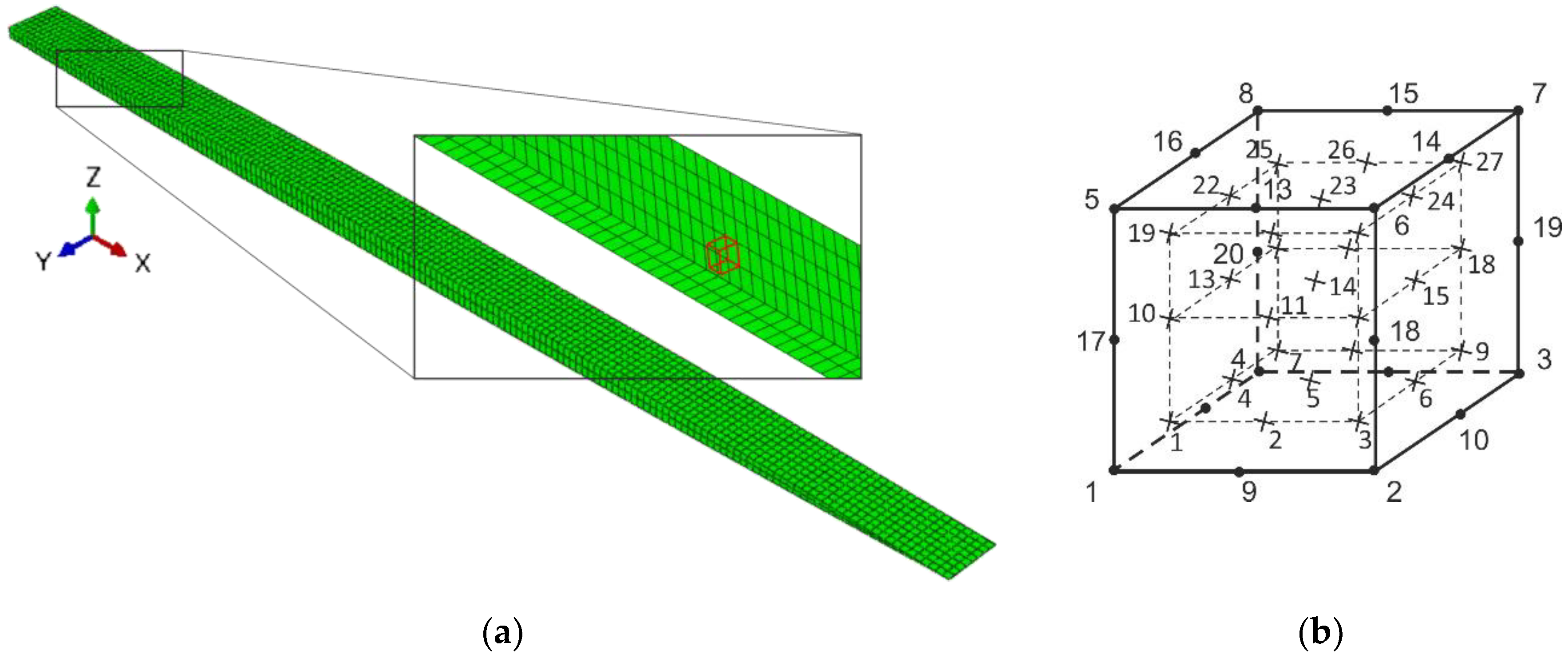
Figure 3.
The geometries of double-parabolic taper beams truncated at the left end: (a) Parabola branches directed to the right; (b) Parabola branches directed to downward.
Figure 3.
The geometries of double-parabolic taper beams truncated at the left end: (a) Parabola branches directed to the right; (b) Parabola branches directed to downward.
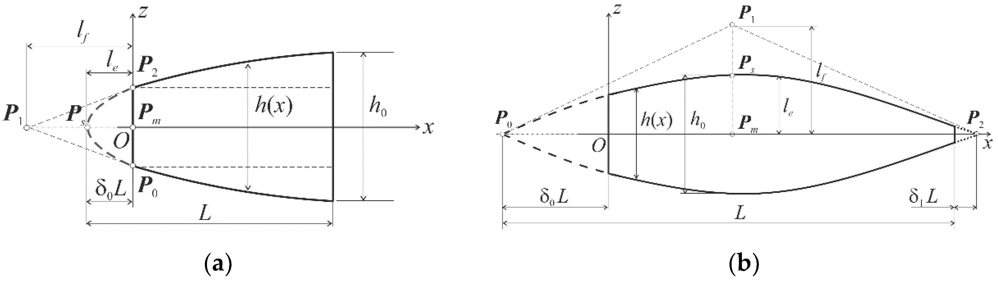
Figure 4.
Mode shapes of truncated AFGM beams with parabolic taper height and constant width obtained from DTM analysis: (a) C-C boundary conditions; (b) C-F boundary conditions.
Figure 4.
Mode shapes of truncated AFGM beams with parabolic taper height and constant width obtained from DTM analysis: (a) C-C boundary conditions; (b) C-F boundary conditions.
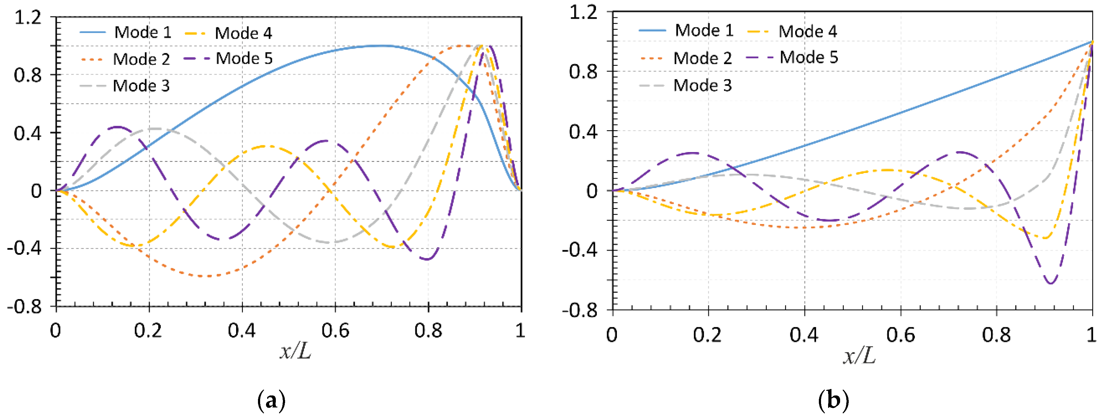

Table 1.
The parameters of uniform beams.
| L, m | , m | , m | , Pa | , Pa | , kg/m3 | ||
|---|---|---|---|---|---|---|---|
| 1 | 0.02 | 0.1 | 2.1×10¹¹ | 0.875×10¹¹ | 0.2 | 0.845 | 7860 |
Table 2.
The natural frequencies of uniform S-S, C-C, and C-F homogeneous beams based on different methods (Hz).
Table 2.
The natural frequencies of uniform S-S, C-C, and C-F homogeneous beams based on different methods (Hz).
| Mode number | S-S | C-C | C-F | ||||||
|---|---|---|---|---|---|---|---|---|---|
| DTM | [47] | Δ*, % | DTM | [47] | Δ, % | DTM | [47] | Δ, % | |
| 1 | 230.7888 | 230.7890 | 6.85E-5 | 500.5870 | 500.5870 | 3.60E-6 | 82.88577 | 82.88600 | 2.82E-5 |
| 2 | 884.4691 | 884.4690 | 1.29E-5 | 1288.763 | 1288.763 | 1.71E-5 | 498.1911 | 498.1910 | 2.90E-5 |
| 3 | 1870.358 | 1870.358 | 1.43E-5 | 2339.160 | 2339.160 | 7.51E-6 | 1315.041 | 1315.041 | 1.36E-5 |
| 4 | 3091.056 | 3091.056 | 4.39E-6 | 3565.013 | 3565.013 | 9.38E-6 | 2394.776 | 2394.776 | 7.00E-6 |
| 5 | 4468.225 | 4468.225 | 9.51E-6 | 4910.439 | 4910.438 | 2.31E-5 | 3658.662 | 3658.662 | 5.88E-6 |
| 6 | 5946.852 | 5946.679 | 2.90E-3 | 6338.321 | 6337.691 | 9.94E-3 | 5044.291 | 5044.277 | 2.85E-3 |
| 7 | 7472.753 | 7489.650 | 2.26 E-1 | 7822.471 | 7821.911 | 7.16E-3 | 6508.492 | 6509.954 | 2.25E-2 |
* .
Table 3.
Dimensionless natural frequencies of uniform cantilever AFGM beams.
| 0 | 1 | 2 | ||||||||||
|---|---|---|---|---|---|---|---|---|---|---|---|---|
| [14] | DTM | DTM* | [14] | DTM | DTM* | [14] | DTM | DTM* | ||||
| 0 | 17.92823 | 17.9268 | 7.98E-3 | 17.78719 | 21.05590 | 21.0543 | 7.59E-3 | 20.89837 | 24.29448 | 24.29265 | 7.53E-3 | 24.11362 |
| 112.3543 | 112.2918 | 5.56E-2 | 106.6048 | 140.9285 | 140.8521 | 5.43E-2 | 133.8822 | 162.7971 | 162.7083 | 5.46E-2 | 154.6099 | |
| 314.5953 | 314.1788 | 1.33E-1 | 280.3868 | 403.4795 | 402.9577 | 1.30E-1 | 360.512 | 462.7162 | 462.1126 | 1.31E-1 | 413.0607 | |
| 616.4812 | 614.9754 | 2.45E-1 | 508.6127 | 795.2794 | 793.3707 | 2.41E-1 | 658.1122 | 909.6774 | 907.4782 | 2.42E-1 | 751.8375 | |
| 1019.088 | 1015.124 | 3.90E-1 | 774.2471 | 1317.894 | 1312.838 | 3.85E-1 | 1004.356 | 1505.584 | 1499.772 | 3.87E-1 | 1145.767 | |
| 1 | 18.89966 | 18.89824 | 7.52E-3 | 18.75921 | 22.29867 | 22.29709 | 7.10E-3 | 22.14241 | 25.73713 | 25.73531 | 7.07E-3 | 25.55769 |
| 124.9620 | 124.8901 | 5.76E-2 | 118.3494 | 158.3713 | 158.2830 | 5.58E-2 | 150.2293 | 182.9067 | 182.8039 | 5.63E-2 | 173.4348 | |
| 355.0148 | 354.5324 | 1.36E-1 | 315.5107 | 460.6318 | 460.0258 | 1.32E-1 | 410.8001 | 527.8895 | 527.1870 | 1.33E-1 | 470.1954 | |
| 698.2161 | 696.4732 | 2.50E-1 | 573.9377 | 911.2419 | 909.0284 | 2.44E-1 | 752.4501 | 1041.633 | 1039.076 | 2.46E-1 | 858.5914 | |
| 1155.920 | 1151.340 | 3.98E-1 | 874.6708 | 1512.257 | 1506.403 | 3.89E-1 | 1150.092 | 1726.572 | 1719.828 | 3.92E-1 | 1310.355 | |
| 2 | 18.99432 | 18.99291 | 7.43E-3 | 18.85473 | 22.45531 | 22.45374 | 6.98E-3 | 22.3005 | 25.92123 | 25.91943 | 6.96E-3 | 25.74348 |
| 127.1780 | 127.1041 | 5.82E-2 | 120.3839 | 162.3684 | 162.2768 | 5.64E-2 | 153.9285 | 187.5542 | 187.4475 | 5.69E-2 | 177.7289 | |
| 363.0379 | 362.5411 | 1.37E-1 | 322.3891 | 475.3808 | 474.7514 | 1.33E-1 | 423.6509 | 544.8226 | 544.0922 | 1.34E-1 | 484.8789 | |
| 714.8085 | 713.0133 | 2.52E-1 | 586.9809 | 941.7464 | 939.4477 | 2.45E-1 | 776.9921 | 1076.597 | 1073.939 | 2.47E-1 | 886.5256 | |
| 1183.930 | 1179.213 | 4.00E-1 | 894.8416 | 1563.728 | 1557.652 | 3.90E-1 | 1188.231 | 1785.535 | 1778.528 | 3.94E-1 | 1353.679 | |
| 3 | 18.97105 | 18.96963 | 7.50E-3 | 18.83099 | 22.45202 | 22.45045 | 6.99E-3 | 22.29715 | 25.91884 | 25.91704 | 6.94E-3 | 25.74104 |
| 126.3443 | 126.2712 | 5.79E-2 | 119.6185 | 162.2392 | 162.1477 | 5.64E-2 | 153.8091 | 187.4615 | 187.3548 | 5.69E-2 | 177.6432 | |
| 359.5311 | 359.0406 | 1.37E-1 | 319.3864 | 474.8301 | 474.2016 | 1.33E-1 | 423.1715 | 544.4325 | 543.7027 | 1.34E-1 | 484.5410 | |
| 707.2811 | 705.5100 | 2.51E-1 | 581.0888 | 940.5708 | 938.2755 | 2.45E-1 | 776.0493 | 1075.765 | 1073.110 | 2.47E-1 | 885.8633 | |
| 1171.009 | 1166.357 | 3.99E-1 | 885.5952 | 1561.717 | 1555.650 | 3.90E-1 | 1186.747 | 1784.113 | 1777.111 | 3.94E-1 | 1352.638 | |
| 4 | 18.97367 | 18.97225 | 7.46E-3 | 18.83369 | 22.44933 | 22.44776 | 7.01E-3 | 22.29437 | 25.92410 | 25.9223 | 6.94E-3 | 25.74647 |
| 126.4718 | 126.3986 | 5.80E-2 | 119.7366 | 162.0943 | 162.0029 | 5.64E-2 | 153.6739 | 187.7400 | 187.6332 | 5.69E-2 | 177.9022 | |
| 360.1566 | 359.6650 | 1.37E-1 | 319.9237 | 474.1105 | 473.4831 | 1.33E-1 | 422.5427 | 545.7931 | 545.0612 | 1.34E-1 | 485.7226 | |
| 708.6890 | 706.9135 | 2.51E-1 | 582.1911 | 938.9675 | 936.6766 | 2.45E-1 | 774.7618 | 1078.791 | 1076.127 | 2.48E-1 | 888.2724 | |
| 1173.481 | 1168.816 | 3.99E-1 | 887.3617 | 1558.918 | 1552.864 | 3.90E-1 | 1184.683 | 1789.389 | 1782.364 | 3.94E-1 | 1356.492 | |
| 5 | - | - | - | - | 22.44994 | 22.44838 | 6.97E-3 | 22.29501 | 25.92274 | 25.92094 | 6.93E-3 | 25.74504 |
| - | - | - | - | 162.1362 | 162.0448 | 5.64E-2 | 153.7134 | 187.6486 | 187.5419 | 5.69E-2 | 177.8163 | |
| - | - | - | - | 474.3503 | 473.7225 | 1.33E-1 | 422.7534 | 545.2794 | 544.5482 | 1.34E-1 | 485.2744 | |
| - | - | - | - | 939.5286 | 937.2362 | 2.45E-1 | 775.2134 | 1077.591 | 1074.931 | 2.48E-1 | 887.3160 | |
| - | - | - | - | 1559.921 | 1553.862 | 3.90E-1 | 1185.423 | 1787.249 | 1780.233 | 3.94E-01 | 1354.929 | |
| 6 | - | - | - | - | - | - | - | - | 25.92296 | 25.92116 | 6.96E-3 | 25.74528 |
| - | - | - | - | - | - | - | - | 187.6670 | 187.5602 | 5.69E-2 | 177.8338 | |
| - | - | - | - | - | - | - | - | 545.3964 | 544.6650 | 1.34E-1 | 485.3772 | |
| - | - | - | - | - | - | - | - | 1077.880 | 1075.218 | 2.48E-1 | 887.5466 | |
| - | - | - | - | - | - | - | - | 1787.776 | 1780.758 | 3.94E-1 | 1355.315 | |
* Dimensionless frequencies of the cantilever AFGM beam with ; ** .
Table 4.
The parameters of uniform exponential-law AFGM beams.
| L, m | , m | , m | , GPa | , kg/m3 | |||
|---|---|---|---|---|---|---|---|
| ZrO2 | Al | ZrO2 | Al | ||||
| 1 | 0.01 | 0.03 | 200 | 70 | 3800 | 2702 | 0.3 |
Table 5.
Dimensionless natural frequencies of uniform exponential-law AFGM beams.
| BCs | -10 | -3 | 0 | 3 | 10 | |||||||||||
|---|---|---|---|---|---|---|---|---|---|---|---|---|---|---|---|---|
| Mode | [11] | DTM | [11] | DTM | [11] | DTM | [11] | DTM | [11] | DTM | ||||||
| S-S | 1 | 9.9225 | 9.8357 | 0.88 | 10.351 | 10.351 | 4.8E-4 | 10.849 | 10.849 | 3.7E-4 | 11.225 | 11.225 | 6.2E-4 | 11.437 | 11.447 | 9.2E-2 |
| 2 | 39.834 | 39.363 | 1.18 | 41.716 | 41.716 | 2.4E-5 | 43.396 | 43.396 | 6.9E-5 | 44.571 | 44.571 | 4.9E-4 | 45.394 | 45.446 | 1.2E-1 | |
| 3 | 89.325 | 89.576 | 0.28 | 93.239 | 93.239 | 2.2E-5 | 96.793 | 96.793 | 3.1E-5 | 99.431 | 99.431 | 1.7E-4 | 101.21 | 101.31 | 9.2E-2 | |
| 4 | 157.50 | 156.01 | 0.94 | 164.07 | 164.07 | 6.1E-6 | 170.22 | 170.22 | 2.4E-5 | 174.87 | 174.87 | 3.0E-4 | 177.98 | 178.17 | 1.1E-1 | |
| C-C | 1 | 24.646 | 24.613 | 0.14 | 24.780 | 24.780 | 1.6E-4 | 24.223 | 24.223 | 1.2E-4 | 23.794 | 23.794 | 7.6E-4 | 23.907 | 23.925 | 7.5E-2 |
| 2 | 65.291 | 65.232 | 0.09 | 66.155 | 66.155 | 1.5E-5 | 66.621 | 66.621 | 4.5E-5 | 66.780 | 66.781 | 1.2E-3 | 67.120 | 67.176 | 8.3E-2 | |
| 3 | 124.53 | 123.97 | 0.44 | 127.04 | 127.04 | 1.6E-5 | 129.55 | 129.55 | 7.7E-6 | 131.09 | 131.09 | 7.5E-4 | 131.94 | 132.03 | 6.8E-2 | |
| 4 | 201.23 | 201.32 | 0.05 | 206.29 | 206.29 | 1.6E-4 | 211.61 | 211.61 | 1.9E-5 | 215.14 | 215.15 | 1.7E-3 | 216.92 | 217.10 | 8.3E-2 | |
* .
Table 6.
Dimensionless natural frequencies of uniform power-law AFGM beams.
| BCs | 1 | 2 | 3 | ||||||||
|---|---|---|---|---|---|---|---|---|---|---|---|
| Mode | [15] | DTM | [15] | DTM | [15] | DTM | |||||
| C-F | 1 | 3.89630 | 3.896310 | 2.57E-4 | 3.88280 | 3.883120 | 8.24E-3 | 3.79570 | 3.797640 | 5.37E-2 | |
| 2 | 15.0505 | 15.05049 | 5.98E-4 | 15.2590 | 15.25982 | 6.03E-3 | 15.2936 | 15.30040 | 4.51E-2 | ||
| 3 | 30.9409 | 30.94087 | 1.20E-3 | 31.6180 | 31.61871 | 3.19E-3 | 31.9962 | 32.00717 | 3.55E-2 | ||
| 4 | 46.3782 | 46.37814 | 1.16E-3 | 47.6349 | 47.63506 | 1.60E-3 | 48.3335 | 48.34427 | 2.37E-2 | ||
| S-S | 1 | 7.84590 | 7.845920 | 2.55E-4 | 7.98730 | 7.988010 | 1.01E-2 | 8.06450 | 8.069630 | 6.49E-2 | |
| 2 | 23.9406 | 23.94060 | 8.35E-4 | 24.2521 | 24.25241 | 2.10E-3 | 24.3532 | 24.35745 | 1.87E-2 | ||
| 3 | 41.6789 | 41.67887 | 1.37E-3 | 42.3024 | 42.30265 | 2.01E-3 | 42.5010 | 42.50566 | 1.24E-2 | ||
| 4 | 53.7111 | 53.71108 | 2.01E-3 | 54.8771 | 54.87722 | 2.22E-3 | 55.3881 | 55.38793 | 1.68E-3 | ||
| C-C | 1 | 12.9065 | 12.90653 | 1.01E-3 | 12.6873 | 12.68758 | 3.78E-3 | 12.6030 | 12.60572 | 2.32E-2 | |
| 2 | 26.7597 | 26.75967 | 1.38E-3 | 26.6416 | 26.64177 | 1.76E-3 | 26.5809 | 26.58381 | 1.21E-2 | ||
| 3 | 43.0417 | 43.04166 | 1.53E-3 | 43.3694 | 43.36938 | 1.34E-3 | 43.4958 | 43.49723 | 4.67E-3 | ||
| 4 | 58.5205 | 58.52006 | 7.86E-4 | 59.2779 | 59.27826 | 1.96E-3 | 59.5726 | 59.57154 | 2.69E-4 | ||
* .
Table 7.
Dimensionless natural frequencies of homogeneous beams with double-parabolic taper.
| BCs | C-C | S-S | F-C | |||||||
|---|---|---|---|---|---|---|---|---|---|---|
| Mode | [2] | DTM | [2] | DTM | [2] | DTM | ||||
| 0.1 | 1 | 14.368 | 14.35795 | 0.07 | 6.3778 | 6.379480 | 0.03 | 5.3883 | 5.371650 | 0.31 |
| 2 | 40.479 | 40.36953 | 0.27 | 27.310 | 27.28302 | 0.10 | 20.699 | 20.55328 | 0.70 | |
| 3 | 80.211 | 79.77238 | 0.55 | 61.023 | 60.84181 | 0.30 | 48.471 | 47.93399 | 1.11 | |
| 0.2 | 1 | 15.972 | 15.9348 | 0.23 | 7.0594 | 7.054580 | 0.07 | 4.8654 | 4.862540 | 0.06 |
| 2 | 44.578 | 44.3374 | 0.54 | 29.395 | 29.32546 | 0.24 | 20.372 | 20.32497 | 0.23 | |
| 3 | 87.897 | 87.0621 | 0.95 | 65.800 | 65.45681 | 0.52 | 49.870 | 49.61366 | 0.51 | |
| 0.3 | 1 | 17.176 | 17.11698 | 0.34 | 7.5823 | 7.575210 | 0.09 | 4.5179 | 4.514900 | 0.07 |
| 2 | 47.701 | 47.32308 | 0.79 | 31.082 | 30.97545 | 0.34 | 20.420 | 20.35704 | 0.31 | |
| 3 | 93.828 | 92.52728 | 1.39 | 69.692 | 69.16329 | 0.76 | 51.543 | 51.17858 | 0.71 | |
| 0.4 | 1 | 18.175 | 18.08114 | 0.52 | 8.0198 | 8.008940 | 0.14 | 4.2660 | 4.262320 | 0.09 |
| 2 | 50.325 | 49.73045 | 1.18 | 32.561 | 32.39500 | 0.51 | 20.592 | 20.50043 | 0.44 | |
| 3 | 98.855 | 96.82087 | 2.06 | 73.098 | 72.27499 | 1.13 | 53.199 | 52.65124 | 1.03 | |
| 0.5 | 1 | 19.044 | 18.89066 | 0.81 | 8.4018 | 8.384520 | 0.21 | 4.0729 | 4.067820 | 0.12 |
| 2 | 52.633 | 51.66934 | 1.83 | 33.904 | 33.63600 | 0.79 | 20.812 | 20.67111 | 0.68 | |
| 3 | 103.30 | 100.0365 | 3.16 | 76.179 | 74.85468 | 1.74 | 54.785 | 53.92227 | 1.57 | |
| 0.6 | 1 | 19.852 | 19.55547 | 1.49 | 8.7443 | 8.71463 | 0.34 | 3.9188 | 3.9112 | 0.19 |
| 2 | 54.718 | 53.06449 | 3.02 | 35.148 | 34.68662 | 1.31 | 21.052 | 20.81738 | 1.11 | |
| 3 | 107.34 | 101.82207 | 5.14 | 79.021 | 76.76144 | 2.86 | 56.296 | 54.84588 | 2.58 | |
| 0.7 | 1 | 20.531 | 20.01665 | 2.51 | 9.0569 | 8.99939 | 0.63 | 3.7922 | 3.77915 | 0.34 |
| 2 | 56.634 | 53.51562 | 5.51 | 36.315 | 35.43022 | 2.44 | 21.299 | 20.85956 | 2.06 | |
| 3 | 111.06 | 96.84761 | 12.80 | 81.676 | 77.40895 | 5.22 | 57.736 | 55.03705 | 4.67 | |
| 0.8 | 1 | 21.186 | 19.98305 | 5.68 | 9.3459 | 9.207100 | 1.49 | 3.6859 | 3.493240 | 5.23 |
| 2 | 58.417 | 43.48449 | 25.6 | 37.419 | 35.37001 | 5.48 | 21.547 | 19.53236 | 9.35 | |
| 3 | 114.54 | 69.00506 | 39.8 | 84.180 | 51.02468 | 39.4 | 59.112 | 63.26979 | 7.03 | |
* .
Table 8.
Dimensionless natural frequencies of cantilever homogeneous beams with parabolic taper height and constant width.
Table 8.
Dimensionless natural frequencies of cantilever homogeneous beams with parabolic taper height and constant width.
| 0.15 | 0.2 | 0.25 | 0.3 | 0.35 | |||||||||||
|---|---|---|---|---|---|---|---|---|---|---|---|---|---|---|---|
| Mode | [3] | DTM | [3] | DTM | [3] | DTM | [3] | DTM | [3] | DTM | |||||
| 1 | 1.050 | 1.05057 | 0.05 | 1.469 | 1.46748 | 0.10 | 1.936 | 1.93539 | 0.03 | 2.465 | 2.46322 | 0.07 | 3.070 | 3.06690 | 0.10 |
| 2 | 7.606 | 7.58803 | 0.24 | 8.958 | 8.93699 | 0.23 | 10.42 | 10.3849 | 0.34 | 12.02 | 11.9846 | 0.29 | 13.83 | 13.7831 | 0.34 |
| 3 | 18.25 | 18.2256 | 0.13 | 20.91 | 20.8092 | 0.48 | 23.79 | 23.6579 | 0.56 | 26.96 | 26.7977 | 0.60 | 30.54 | 30.3304 | 0.69 |
| 4 | 32.54 | 31.9653 | 1.77 | 36.96 | 36.6841 | 0.75 | 41.73 | 41.3659 | 0.87 | 46.99 | 46.5406 | 0.96 | 52.92 | 52.3541 | 1.07 |
| 0.4 | 0.45 | 0.5 | 0.55 | 0.6 | |||||||||||
| 1 | 3.770 | 3.76591 | 0.11 | 4.593 | 4.58701 | 0.13 | 5.576 | 5.56729 | 0.16 | 6.772 | 6.76070 | 0.17 | 8.263 | 8.24726 | 0.19 |
| 2 | 15.91 | 15.8416 | 0.43 | 18.32 | 18.2384 | 0.45 | 21.18 | 21.0814 | 0.47 | 24.65 | 24.5248 | 0.51 | 28.96 | 28.7980 | 0.56 |
| 3 | 34.63 | 34.3716 | 0.75 | 39.40 | 39.0763 | 0.82 | 45.05 | 44.6586 | 0.87 | 51.9 | 51.4115 | 0.94 | 60.41 | 59.7941 | 1.02 |
| 4 | 59.70 | 59.0060 | 1.16 | 67.61 | 66.7478 | 1.28 | 76.98 | 75.9204 | 1.38 | 88.34 | 87.0392 | 1.47 | 102.4 | 100.825 | 1.54 |
| 0.65 | 0.7 | 0.75 | 0.8 | 0.85 | |||||||||||
| 1 | 10.17 | 10.1532 | 0.16 | 12.72 | 12.6888 | 0.25 | 16.27 | 16.2322 | 0.23 | 21.60 | 21.5566 | 0.20 | 30.47 | 30.3768 | 0.31 |
| 2 | 34.47 | 34.2610 | 0.61 | 41.78 | 41.5124 | 0.64 | 51.99 | 51.6294 | 0.69 | 67.26 | 66.6661 | 0.88 | 92.66 | 91.9427 | 0.77 |
| 3 | 71.29 | 70.5089 | 1.10 | 85.72 | 84.7297 | 1.16 | 105.9 | 104.568 | 1.26 | 136.0 | 134.452 | 1.14 | 186.2 | 183.606 | 1.39 |
| 4 | 120.5 | 118.443 | 1.71 | 144.4 | 141.823 | 1.78 | 177.8 | 174.436 | 1.89 | 227.8 | 222.612 | 2.28 | 310.9 | 304.354 | 2.11 |
* .
Table 9.
The parameters of curvilinearly non-uniform AFGM beams.
| Material | , GPa | , kg/m3 | L, m | , m | , m | , m | , m | |
|---|---|---|---|---|---|---|---|---|
| Aluminum | 70 | 2700 | 0.3 | 1 | 0.2 | 0.2 | 0.04 | 0.1 |
| Steel | 348.43 | 2370 | 0.24 | |||||
| Si3N4 | 201.04 | 8166 | 0.33 |
Table 10.
Natural frequencies, Hz, of the C-C AFGM beams with curvilinear taper height and constant width.
Table 10.
Natural frequencies, Hz, of the C-C AFGM beams with curvilinear taper height and constant width.
| AFGM | Model | 0 | 1 | 5 | |||||||
|---|---|---|---|---|---|---|---|---|---|---|---|
| Mode | [29] | DTM | [29] | DTM | [29] | DTM | |||||
| Type 2 | Plump | 1 | 889.39 | 887.304 | 0.23 | 891.48 | 889.589 | 0.21 | 997.39 | 1002.94 | 0.56 |
| 2 | 1889.1 | 2034.36 | 7.69 | 1894.4 | 2041.25 | 7.75 | 2025.3 | 2203.40 | 8.79 | ||
| Slender | 1 | 800.93 | 779.141 | 2.72 | 805.63 | 783.893 | 2.70 | 920.25 | 899.469 | 2.26 | |
| 2 | 1774.6 | 1728.28 | 2.61 | 1778.8 | 1732.06 | 2.63 | 1882.4 | 1838.13 | 2.35 | ||
| Type 3 | Plump | 1 | 2128.3 | 2133.71 | 0.25 | 1229.4 | 1226.23 | 0.26 | 947.74 | 947.074 | 0.07 |
| 2 | 4532.2 | 4911.19 | 8.36 | 2632.4 | 2837.54 | 7.79 | 2036.2 | 2199.87 | 8.04 | ||
| Slender | 1 | 1906.2 | 1865.29 | 2.15 | 1108.2 | 1078.24 | 2.70 | 851.24 | 828.860 | 2.63 | |
| 2 | 4239.8 | 4151.87 | 2.07 | 2471.8 | 2406.75 | 2.63 | 1902.5 | 1856.66 | 2.41 | ||
* .
Table 11.
Dimensionless natural frequencies of truncated AFGM beams with parabolic taper height and constant width.
Table 11.
Dimensionless natural frequencies of truncated AFGM beams with parabolic taper height and constant width.
| BCs | 0.2 | 0.4 | 0.6 | ||||||||||
|---|---|---|---|---|---|---|---|---|---|---|---|---|---|
| Mode | [23] | FEM | DTM | [23] | FEM | DTM | [23] | FEM | DTM | ||||
| C-C | 1 | 18.4750 | 18.8461 | 18.5033 | 0.15 | 16.423 | 16.7328 | 16.4583 | 0.21 | 14.1591 | 14.7828 | 14.2013 | 0.30 |
| 2 | - | 53.7872 | 51.5889 | 4.09 | - | 47.1474 | 46.5676 | 1.23 | - | 42.3017 | 40.8931 | 3.33 | |
| 3 | - | 105.999 | 101.332 | 4.40 | - | 93.1729 | 92.1155 | 1.13 | - | 84.2618 | 81.5879 | 3.17 | |
| 4 | - | 175.772 | 167.090 | 4.94 | - | 154.114 | 152.461 | 1.07 | - | 139.905 | 135.640 | 3.05 | |
| 5 | - | 261.850 | 248.400 | 5.14 | - | 229.652 | 227.231 | 1.05 | - | 208.997 | 202.736 | 3.00 | |
| C-F | 1 | 2.5715 | 2.71073 | 2.57115 | 0.01 | 2.7594 | 2.94885 | 2.75933 | 0.00 | 3.0151 | 3.17381 | 3.0146 | 0.02 |
| 2 | - | 18.8484 | 18.0533 | 4.22 | - | 18.3961 | 17.5276 | 4.72 | - | 18.0266 | 17.0113 | 5.63 | |
| 3 | - | 54.3519 | 51.7463 | 4.79 | - | 49.5819 | 48.3800 | 2.42 | - | 46.8092 | 44.6929 | 4.52 | |
| 4 | - | 107.161 | 101.628 | 5.16 | - | 95.5807 | 94.1178 | 1.53 | - | 88.8564 | 85.6122 | 3.65 | |
| 5 | - | 177.343 | 167.573 | 5.51 | - | 156.448 | 154.637 | 1.16 | - | 142.196 | 139.622 | 1.81 | |
* .
Table 12.
Dimensionless natural frequencies of curvilinear taper C-C AFGM beams with various exponential law (3) parameters.
Table 12.
Dimensionless natural frequencies of curvilinear taper C-C AFGM beams with various exponential law (3) parameters.
| Model | a | 0.2 | 0.5 | 0.8 | 1.0 | ||||||||
|---|---|---|---|---|---|---|---|---|---|---|---|---|---|
| [29] | DTM | DTM* | [29] | DTM | DTM* | [29] | DTM | DTM* | [29] | DTM | DTM* | ||
| Plump | 0 | 1.0975 | 1.09493 | 1.03005 | 1.0975 | 1.09493 | 1.03005 | 1.0975 | 1.09493 | 1.03005 | 1.0975 | 1.09493 | 1.03005 |
| 2.3311 | 2.51039 | 2.41452 | 2.3311 | 2.51039 | 2.41452 | 2.3311 | 2.51039 | 2.41452 | 2.3311 | 2.51039 | 2.41452 | ||
| 0.5 | 1.0975 | 1.09495 | 1.03006 | 1.0977 | 1.09509 | 1.03012 | 1.0979 | 1.09669 | 1.03025 | 1.0981 | 1.09560 | 1.03037 | |
| 2.3312 | 2.51047 | 2.41461 | 2.3316 | 2.51092 | 2.41510 | 2.3322 | 2.51583 | 2.41601 | 2.3328 | 2.51252 | 2.41685 | ||
| 1 | 1.0976 | 1.09503 | 1.03010 | 1.0981 | 1.09560 | 1.03037 | 1.0991 | 1.09923 | 1.03093 | 1.1001 | 1.09774 | 1.03149 | |
| 2.3314 | 2.51073 | 2.41489 | 2.3328 | 2.51252 | 2.41685 | 2.3353 | 2.52559 | 2.42049 | 2.3377 | 2.51889 | 2.42384 | ||
| 2 | 1.0979 | 1.09536 | 1.03025 | 1.1001 | 1.09774 | 1.03149 | 1.1047 | 1.10274 | 1.03446 | 1.1095 | 1.10799 | 1.03796 | |
| 2.3322 | 2.51175 | 2.41601 | 2.3377 | 2.51889 | 2.42384 | 2.348 | 2.53212 | 2.43829 | 2.3575 | 2.54429 | 2.45154 | ||
| 5 | 1.1001 | 1.09774 | 1.03149 | 1.1181 | 1.11733 | 1.04478 | 1.1689 | 1.17175 | 1.09083 | 1.2308 | 1.23763 | 1.15183 | |
| 2.3377 | 2.51889 | 2.42384 | 2.3725 | 2.56324 | 2.47209 | 2.4379 | 2.6446 | 2.55945 | 2.4992 | 2.71898 | 2.63835 | ||
| Slen der | 0 | 0.9883 | 0.96145 | 1.06330 | 0.9883 | 0.96145 | 1.06330 | 0.9883 | 0.96145 | 1.06330 | 0.9883 | 0.96145 | 1.06330 |
| 2.1899 | 2.13269 | 2.27063 | 2.1899 | 2.13269 | 2.27063 | 2.1899 | 2.13269 | 2.27063 | 2.1899 | 2.13269 | 2.27063 | ||
| 0.5 | 0.9884 | 0.96151 | 1.06337 | 0.9887 | 0.96292 | 1.06368 | 0.9893 | 0.96239 | 1.06427 | 0.9898 | 0.96292 | 1.06482 | |
| 2.1899 | 2.13273 | 2.27063 | 2.1902 | 2.13385 | 2.27066 | 2.1907 | 2.13343 | 2.27071 | 2.1912 | 2.13385 | 2.27076 | ||
| 1 | 0.9886 | 0.96169 | 1.06355 | 0.9898 | 0.96292 | 1.06482 | 0.9921 | 0.96521 | 1.06718 | 0.9941 | 0.96732 | 1.06936 | |
| 2.1901 | 2.13287 | 2.27065 | 2.1912 | 2.13385 | 2.27076 | 2.1932 | 2.13567 | 2.27101 | 2.1951 | 2.13735 | 2.27128 | ||
| 2 | 0.9893 | 0.96239 | 1.06427 | 0.9941 | 0.96732 | 1.06936 | 1.0032 | 0.97648 | 1.07883 | 1.0116 | 0.98496 | 1.08759 | |
| 2.1907 | 2.13343 | 2.27071 | 2.1951 | 2.13735 | 2.27128 | 2.2032 | 2.14468 | 2.27284 | 2.2108 | 2.15152 | 2.27483 | ||
| 5 | 0.9941 | 0.96732 | 1.06936 | 1.0248 | 0.99839 | 1.10130 | 1.0821 | 1.05618 | 1.16083 | 1.1356 | 1.10994 | 1.21554 | |
| 2.1951 | 2.13735 | 2.27128 | 2.2226 | 2.16369 | 2.27892 | 2.2800 | 2.21822 | 2.30846 | 2.3998 | 2.26823 | 2.35005 | ||
* Curvilinear double taper beam.
Table 13.
Dimensionless natural frequencies of curvilinear taper C-C AFGM beams with various power law (4) parameters.
Table 13.
Dimensionless natural frequencies of curvilinear taper C-C AFGM beams with various power law (4) parameters.
| Model | b | 0.2 | 0.5 | 0.8 | 1.0 | ||||||||
|---|---|---|---|---|---|---|---|---|---|---|---|---|---|
| [29] | DTM | DTM* | [29] | DTM | DTM* | [29] | DTM | DTM* | [29] | DTM | DTM* | ||
| Plump | 0 | 1.1029 | 1.10568 | 1.04031 | 1.1029 | 1.10568 | 1.04031 | 1.1029 | 1.10569 | 1.04031 | 1.1029 | 1.10569 | 1.04031 |
| 2.3486 | 2.54497 | 2.44810 | 2.3486 | 2.54497 | 2.44810 | 2.3486 | 2.54498 | 2.44813 | 2.3486 | 2.54497 | 2.44813 | ||
| 0.5 | 1.0270 | 1.02926 | 0.96840 | 0.9236 | 0.92519 | 0.87025 | 0.8254 | 0.82580 | 0.77672 | 0.7529 | 0.75141 | 0.70703 | |
| 2.1870 | 2.36872 | 2.27858 | 1.9669 | 2.12879 | 2.04736 | 1.7563 | 1.89754 | 1.82512 | 1.5969 | 1.72072 | 1.65589 | ||
| 1 | 0.9653 | 0.96706 | 0.90989 | 0.8139 | 0.81428 | 0.76616 | 0.7002 | 0.69935 | 0.65802 | 0.6371 | 0.63543 | 0.59782 | |
| 2.0571 | 2.22708 | 2.14243 | 1.7383 | 1.87906 | 1.80811 | 1.4981 | 1.61675 | 1.55635 | 1.3641 | 1.47041 | 1.41596 | ||
| 2 | 0.8708 | 0.87183 | 0.82031 | 0.6878 | 0.68729 | 0.64668 | 0.5897 | 0.58870 | 0.55389 | 0.5512 | 0.55024 | 0.51771 | |
| 1.8597 | 2.01193 | 1.93575 | 1.4761 | 1.59425 | 1.53483 | 1.2703 | 1.37125 | 1.32095 | 1.1901 | 1.28514 | 1.23845 | ||
| 5 | 0.7083 | 0.70814 | 0.66630 | 0.5512 | 0.55045 | 0.51792 | 0.5044 | 0.50397 | 0.47425 | 0.4911 | 0.49077 | 0.46188 | |
| 1.5204 | 1.64301 | 1.58161 | 1.1883 | 1.28345 | 1.23660 | 1.0864 | 1.17376 | 1.13122 | 1.0551 | 1.13997 | 1.09864 | ||
| Slen der | 0 | 0.9878 | 0.96659 | 1.06906 | 0.9878 | 0.96659 | 1.06906 | 0.9878 | 0.96659 | 1.06906 | 0.9878 | 0.96659 | 1.06906 |
| 2.1970 | 2.15149 | 2.29122 | 2.1970 | 2.15149 | 2.29122 | 2.1970 | 2.15149 | 2.29122 | 2.1970 | 2.15149 | 2.29122 | ||
| 0.5 | 0.9203 | 0.90015 | 0.99556 | 0.8285 | 0.81359 | 0.89622 | 0.7420 | 0.72427 | 0.80065 | 0.6790 | 0.66130 | 0.73109 | |
| 2.0466 | 2.00327 | 2.13265 | 1.8421 | 1.74851 | 1.92080 | 1.6476 | 1.60620 | 1.70524 | 1.5028 | 1.46410 | 1.54951 | ||
| 1 | 0.8654 | 0.84606 | 0.93568 | 0.7309 | 0.71349 | 0.78886 | 0.6302 | 0.61411 | 0.67858 | 0.5743 | 0.55882 | 0.61731 | |
| 1.9255 | 1.88386 | 2.00444 | 1.6286 | 1.59073 | 1.68759 | 1.4054 | 1.37004 | 1.44874 | 1.2809 | 1.24838 | 1.31629 | ||
| 2 | 0.7812 | 0.76321 | 0.84391 | 0.6183 | 0.60271 | 0.66606 | 0.5307 | 0.51674 | 0.57062 | 0.4959 | 0.48271 | 0.53300 | |
| 1.7411 | 1.70209 | 1.80889 | 1.3828 | 1.34864 | 1.42756 | 1.1895 | 1.15997 | 1.22235 | 1.1133 | 1.08328 | 1.14099 | ||
| 5 | 0.6363 | 0.62055 | 0.68581 | 0.4955 | 0.48246 | 0.53250 | 0.4532 | 0.44121 | 0.48651 | 0.4411 | 0.42951 | 0.47381 | |
| 1.4235 | 1.38932 | 1.47301 | 1.1113 | 1.08346 | 1.15111 | 1.015 | 0.99219 | 1.06980 | 0.9859 | 0.96212 | 1.03009 | ||
* Curvilinear double taper beam.
Table 14.
Dimensionless natural frequencies of curvilinear taper AFGM beams with various boundary conditions.
Table 14.
Dimensionless natural frequencies of curvilinear taper AFGM beams with various boundary conditions.
| AFGM | Model | BCs | C-C | C-S | C-F | S-S | ||||||||
|---|---|---|---|---|---|---|---|---|---|---|---|---|---|---|
| Mode | [29] | DTM | DTM* | [29] | DTM | DTM* | [29] | DTM | DTM* | [29] | DTM | DTM* | ||
| Type 2 | Plump | 1 | 1.1001 | 1.09774 | 1.03149 | 0.8392 | 0.83336 | 0.80370 | 0.1669 | 0.16736 | 0.16262 | 0.6856 | 0.67765 | 0.66811 |
| 2 | 2.3377 | 2.51889 | 2.42384 | 1.5533 | 2.31624 | 2.25450 | 0.9638 | 1.13797 | 1.12997 | 1.8524 | 2.16694 | 2.13405 | ||
| Slender | 1 | 0.9941 | 0.98513 | 1.06936 | 0.5764 | 0.56832 | 0.58619 | 0.1070 | 0.10628 | 0.09795 | 0.3468 | 0.34744 | 0.33893 | |
| 2 | 2.1951 | 2.15107 | 2.27128 | 1.7610 | 1.74672 | 1.89129 | 0.7314 | 0.7207 | 0.72082 | 1.3943 | 1.4032 | 1.43892 | ||
| Type 3 | Plump | 1 | 0.6371 | 0.63543 | 0.59782 | 0.5215 | 0.51757 | 0.49565 | 0.1460 | 0.14617 | 0.13912 | 0.4070 | 0.40223 | 0.39643 |
| 2 | 0.8972 | 1.47041 | 1.41596 | 0.9537 | 1.36093 | 1.32281 | 0.6423 | 0.74588 | 0.73694 | 1.0946 | 1.27727 | 1.25659 | ||
| Slender | 1 | 0.5743 | 0.55882 | 0.61731 | 0.3808 | 0.37381 | 0.39302 | 0.1008 | 0.09998 | 0.09508 | 0.2065 | 0.20703 | 0.2028 | |
| 2 | 1.2809 | 1.24838 | 1.31629 | 1.0547 | 1.0332 | 1.06555 | 0.4992 | 0.48937 | 0.49201 | 0.8293 | 0.82974 | 0.82545 | ||
* Curvilinear double taper beam.
Disclaimer/Publisher’s Note: The statements, opinions and data contained in all publications are solely those of the individual author(s) and contributor(s) and not of MDPI and/or the editor(s). MDPI and/or the editor(s) disclaim responsibility for any injury to people or property resulting from any ideas, methods, instructions or products referred to in the content. |
© 2024 by the authors. Licensee MDPI, Basel, Switzerland. This article is an open access article distributed under the terms and conditions of the Creative Commons Attribution (CC BY) license (http://creativecommons.org/licenses/by/4.0/).
Copyright: This open access article is published under a Creative Commons CC BY 4.0 license, which permit the free download, distribution, and reuse, provided that the author and preprint are cited in any reuse.


