
Submitted:
10 July 2024
Posted:
12 July 2024
You are already at the latest version
Abstract
ATTO 565, a Rhodamine-type dye, has garnered significant attention due to its remarkable optical properties, such as a high fluorescence quantum yield, it is a relatively stable structure, and has low biotoxicity. ATTO 565 has found extensive applications in combination with microscopy technology. In this review, the chemical and optical properties of ATTO 565 are introduced, along with the principles behind them. Then, the functionality of ATTO 565 in confocal microscopy, stimulated emission depletion (STED) microscopy, single-molecule tracking (SMT) techniques, and fluorescence correlation spectroscopy (FCS) is discussed. These studies demonstrate that ATTO 565 plays a crucial role in areas such as biological imaging and single-molecule localization, thus warranting further in-depth investigation. Finally, we present some prospects and concepts for the future applications of ATTO 565 in the fields of biocompatibility and metal ion detection.
Keywords:
high-resolution microscopy
; fluorescent Rhodamine dye
; stimulated emission depletion microscopy
; fluorescent labeling
; fluorescence correlation spectroscopy
; 3D single molecule tracking
1. Introduction
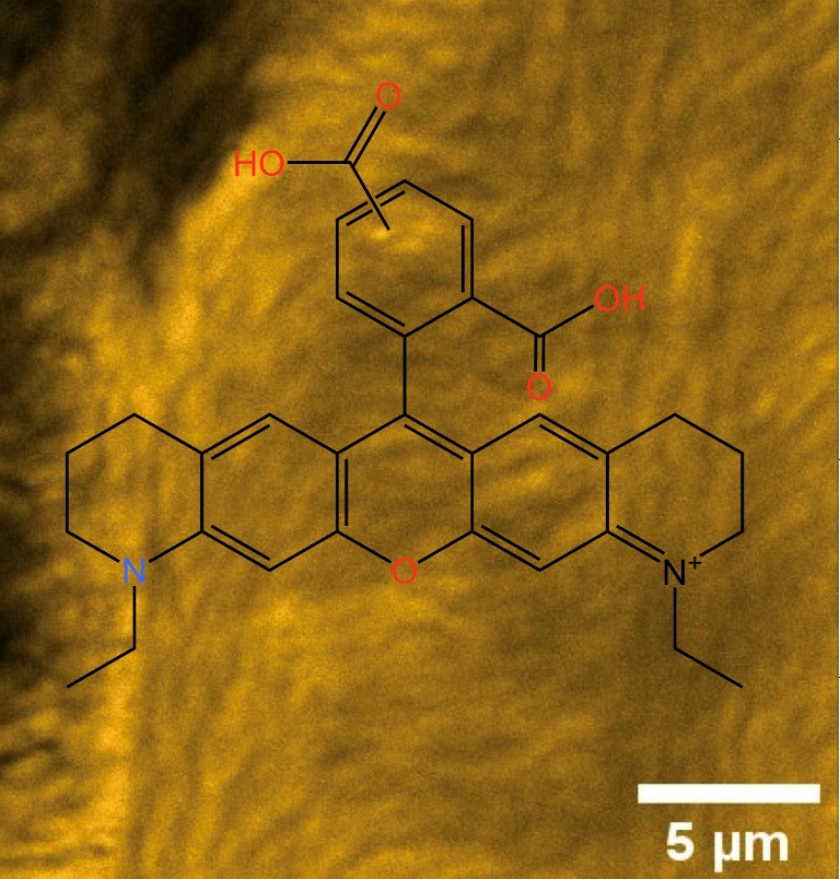
Fluorescent dyes are important tools across various domains such as biological imaging, cell tracking, and molecular probing. They play an essential role in advancing modern life sciences and materials science. In recent years, there has been a continuous surge in the research and development of novel fluorescent dyes [1]. As a type of Rhodamine dye, ATTO 565 shows notable traits including intense absorption, high fluorescence quantum yield, and exceptional thermal and photo-stability [2]. These remarkable properties have rendered it extensively applicable in the field of single-molecule detection applications and high-resolution microscopy [3]. The structure of ATTO 565 is shown in Figure 1(A). ATTO 565 is used in stimulated emission depletion (STED) microscopy. To overcome Abbe's diffraction limit, stimulated emission is employed to deplete the fluorescent state. This generates focal regions of molecular excitation significantly smaller than the diffraction limit and significantly increases the resolution [4]. ATTO 565 is a suitable fluorescent dye in STED due to its superior performance. Wildanger et al. used ATTO 565 as a fluorescent labeling dye for immunofluorescence staining of mammalian PtK2 cells. Compared to the confocal image, the STED image clearly shows the structures and spaced fibers of cells [5], as shown in Figure 1(B) and (C).
Besides its contribution to STED, ATTO 565 is also used in visually evaluating the drug delivery potential and studying the mechanism of drug delivery [6]. All these applications reveal that ATTO 565 is a promising fluorescent dye with great potential. In this review, the applications of ATTO 565 in various types of microscopy techniques are explored, revealing the significant capabilities of ATTO 565 in assisting researchers to explore the microscopic world.
2. The Properties of the ATTO 565 Dye
2.1. Chemical Properties
Rhodamine dyes, as organic compounds, are a type of fluorescent dyes commonly used in biological, chemical, and fluorescence microscopy research. The molecular structures of Rhodamine dyes are based on a xanthene core which acts as the chromophore [7]. The primary differences between Rhodamine dyes lie in the various substituents on the xanthene framework. For example, there are two dimethylamino substituents on the xanthene core of Rhodamine B and two ethylamine groups for ATTO 532, as shown in Figure 2(A) and (B).
There is a delocalized π system in the xanthene structure. When a molecule absorbs a photon, it undergoes a π → π* transition, subsequently emitting fluorescence during the de-excitation process [7]. Most rhodamine dyes have a carboxyl substituent or a similar substituent near the xanthene ring. In an alkaline environment, the carboxyl group loses a proton, leading to a nucleophilic attack on the central carbon atom to form a five-membered lactone structure. This closed-form structure interrupts the xanthene chromophore, causing rhodamine dyes not to exhibit absorption or emission peaks within the visible light range. In comparison, in acidic or neutral environments, the xanthene structure remains in its original state, which is referred to as the open form. The open form of Rhodamine demonstrates superior fluorescence performance [8]. The switch of ATTO 565 between open and closed forms is shown in Figure 2(C) [9]. This is exactly the principle of how rhodamine dye acts as a pH meter within the fluorescent sensors field [9]. The structural conformational changes between the open and closed forms allow Rhodamine dyes to be used in different experimental conditions because their fluorescent properties can be controlled by altering pH or light exposure conditions, and this makes them highly valuable in fields such as cell biology, molecular biology, and biological imaging [10].
Lampidis et al. have already demonstrated that certain Rhodamine dyes exhibit selective accumulative biotoxicity to cancer cells without harming normal cells, due to the higher plasma membrane potential of carcinoma cells. This implies that ATTO 565 also holds significant potential for in vivo experiments [11].
2.2. Optical Properties
The fundamental characteristics of ATTO 565 were assessed by ATTO-TEC GmbH [12]. The emission and absorption spectra of ATTO 565 are shown in Figure 3(A). The wavelength of the strongest absorption peak is ~564 nm, which is the origin of its name. The wavelength of the emission maximum is 590 nm. There is a clear Stokes shift for ATTO 565. This makes the use of ATTO 565 convenient for fluorescence excitation experiments as it reduces the influence on the emission spectrum by the excitation light. The molar absorptivity of ATTO 565 is 1.2 x 10⁵ M-1 cm-1. This high absorptivity coefficient indicates that ATTO 565 possesses high sensitivity, enabling it to effectively absorb light even at low concentrations. The fluorescence quantum yield of ATTO 565 is 90%, which implies that ATTO 565 efficiently converts the absorbed energy into fluorescence emission, even under low concentration conditions of the analyte, producing a strong fluorescence signal. The optical data are shown in Table 1.
To gain insights into the properties of the dye, researchers employed single-molecule fluorescence spectroscopy to acquire typical emission intensity time traces of individual ATTO 565 molecules on a glass surface in a normal environment. The fluorescence time trace of dye 565 is shown in Figure 3(B) [13]. The intensity fluctuations are obvious. Several intermittencies happened before the final photobleaching at 105 s. During these intermittencies, the molecule stops emitting fluorescence, and this change of intensity is usually named “blinking”. When the trace is magnified at 28 s, one blinking event which lasts 330 ms is shown in Figure 3(C) [13].
Some possible explanations for the blinking phenomenon have been proposed. One common explanation is the three electronic state theory shown in Figure 4. When the molecule absorbs the energy from the photon, it is excited from ground state S0 to the first excited state S1. After a very short excited state lifetime, it goes back to the S0 state with the emission of radiation. This is the reason for the “on time” of fluorescent dye molecules. However, there’s a possibility that the molecule converts from the S1 to the triplet excited state T1. It will stay in T1 with a longer excited state lifetime than in S1 since conversion back to the ground state from T1 is spin forbidden. In the end, the molecule relaxes to S0. This pathway proceeds entirely through intersystem crossing and is completely non-fluorescent, manifesting as a molecular dark state on a macroscopic scale. Also, intensity fluctuations in some cases may result from environmental variations, such as minor temperature changes, which can impact the absorption spectrum [14].
Further research, however, has revealed some evidence suggesting that the blinking phenomenon of ATTO 565 may not necessarily follow the three electronic state theory. Yeow et al. used the data of fluorescence intensity time trace to make the autocorrelation curve for ATTO 565 with an excitation wavelength of 543 nm [13]. Figure 5 is a schematic representation of the simulated autocorrelation function of fluorescent dye fluorescence, which closely resembles the actual experimental results of ATTO 565. Fitting the curve using Formula (1) allows us to obtain some key parameters. Using the formula brought forward by Krichevsky et al. to fit the curve [15], the average triplet state lifetime yielded a value of 6 μs. A more specific explanation of the autocorrelation curve is in section 3.4. In Formula (1), Neff denotes the average number of fluorescent molecules in ROI, F is the fraction of molecules that are in the triplet state, and w is a parameter about the volume of the ROI.
G(t) = { [ 1 – F + Fexp ( - t / τtri ) ] / [ ( 1 – F ) Neff ] } × [ ( 1 + t / τdiff )( 1 + t / w2 τdiff )0.5 ]-1
However, the measured dark state time of a single molecule in Figure 3(C) is 3×10⁵ μs, and it’s tens of thousands of times bigger than τtri. This indicates that the three electron states may not well explain the blinking of ATTO 565.
Another proposed theory is based on four electronic states shown in Figure 6. After being excited to S1, the molecule has two pathways to reach the dark state D. One involves intersystem crossing to T1 followed by electron tunneling to the dark state, while the other pathway directly involves electron tunneling to the dark state. Yeow et. al. conducted Monte Carlo simulations to test the validity of the dual-pathway model and found that reproducing the observed fluorescence intermittency behavior in the experiments requires the simultaneous consideration of both pathway 1 and pathway 2 [13].
As a fluorescent dye, ATTO 565 will suffer photobleaching under high-intensity lighting. Researchers put ATTO 565 molecules in different intensity lighting conditions and tested their bleaching time histogram as shown in Figure 7. In the tested range, it can be observed that the degree of photobleaching increases with the increasing light intensity [13].
To further elucidate the mechanism of photo-bleaching in ATTO 565, researchers monitored changes in fluorescence intensity over time in different media. The groups with air condition exhibit biexponential decay and the group with nitrogen condition exhibits monoexponentially decay as shown in Figure 8(A). A four-electron energy level hypothesis has been proposed to explain biexponential decay as shown in Figure 8(B). There are two different pathways of photobleaching. In the first one, the molecule will form a radical D state, and the bleaching rate is determined from the rate of molecule transfer from T1 to B1 which is the bleached state, and D to B2. In the other pathway, the molecule wouldn’t form a D state, and the bleaching rate is determined only by kb. From the macroscopic perspective, the decay rate of ATTO 565 molecular populations in air is determined by two rate constants due to the two pathways.
The bleaching mechanism in the air is related to oxygen. “The quenching mechanism is most likely due to an oxygen-dependent reaction whereby reactive singlet oxygen (1O2) formed from the reaction between T1 and triplet oxygen (3O2) can attack and eventually destroy the molecules.”(see p. 1732), as stated by Yeow et al. When there is a lack of oxygen in the environment, bleaching may occur due to reactions with the surrounding matrix in T1/D [13].
3. The Application of ATTO 565 in Microscopy
3.1. Applications of ATTO 565 in Confocal Microscopy
3.1.1. Utilizing ATTO 565 for Assessing the Effectiveness of Nanostructures
ATTO 565 can be directly employed in fluorescent imaging of nanometer-sized structures. The concept of "Lab-on-a-chip" represents a groundbreaking approach that consolidates various chemical and biological analysis functions onto a single compact chip, designed for handling extremely minute liquid volumes, down to less than a pico-liter. This chip comprises numerous microchannels, necessitating a convenient method for assessing the effectiveness of these microchannels [16]. Due to its excellent fluorescence performance, ATTO 565 stands out in fulfilling this requirement.
Wang et al. utilized ATTO 565 in conjunction with a confocal microscope to assess the performance of Proton Beam Writing (PBW), a technique for fabricating and etching micro and nanostructures [17]. Poly(methyl methacrylate) (PMMA) was selected as the material of the whole nanofluidic structure because it exhibits good reproducibility in PBW [18], and its transparency facilitates fluorescence detection. They initiated the process by employing a 2 MeV photon beam to create nanofluid channels with a width of 100 nm and a depth of 2 μm, followed by the design of inlet and outlet channels. Subsequently, a 1 nM ATTO 565 solution was introduced into the nanosystem using a syringe pump. Laser lines, generated at 543 nm with a HeNe laser, were then employed to excite ATTO 565. Fluorescence correlation spectroscopy (FCS) was utilized to determine the time it takes for the liquid to first flow out of the nanoscale pipeline and to completely flow out, aiding in guiding the practical applications of nanoscale pipelines. Additionally, confocal microscopy captured side-view images of the nanoscale pipeline. The result is presented in Figure 9, where it can be observed that the diameter of the nanoscale pipeline is approximately 100 nanometers, and its shape is perfectly straight.
3.1.2. Utilizing ATTO 565 for Assessing the Effectiveness of Biostructures
ATTO 565 is commonly utilized in biology to label and visualize biological molecules, cell structures, and biological processes for research and monitoring purposes. For example, Roizard et al. employed ATTO 565 to visualize the binding of G-protein receptors (GPCRs) to G proteins on the kidney cell membrane and determined their reaction kinetics parameters [19]. GPCRs are a class of protein receptors widely present on the cell membrane that can interact with G proteins [20]. To introduce fluorescent dyes like ATTO 565 into the membrane and measure the reactions using microscopes effectively, it is necessary to transform the cell membrane into solid-supported membranes, which involves fixing biological membranes on a solid surface. Researchers achieved this by immobilizing cells on agarose beads coated with wheat germ agglutinin (WGA) and then flipping the cell membrane inside-out onto the agarose beads through stirring, as depicted in Figure 10(A). WGA is a type of protein that can bind with glycans on the plasma membrane and subsequently fix the cell membrane, facilitating ligand binding. Within the membrane, A2AR fused with mCitrine (A2AR-Citrine) are located. A2AR represents a type of GPCR, and citrine is employed as a marker. These components are generated by a plasmid within the cell.
The A2A-AR agonist (APEC) is combined with ATTO 633 [21]. ATTO 633 is another Rhodamine dye like ATTO 565 but with different absorption and excitation wavelengths. The G protein Gαβγ is combined with tris-NTA-Pro8-ATTO 565, a fluorescent probe described in detail in Section 3.2.3. Three fluorescent dyes were employed in this experiment to clearly distinguish GPCR, ligand, and G protein. Firstly, the membrane was exposed to a 60 nM APEC-ATTO 633 solution, followed by exposure to 17 nM Gαβγ-ATTO 565, and fluorescent data recording commenced. The excitation wavelengths for ATTO 633 and ATTO 565 are 633 nm and 561 nm, respectively. Confocal microscope images are presented in Figure 10(B) and (C), confirming successful binding of the ligand and G protein to the cell membrane. Figure 10(D) illustrates the binding status of the fluorescent dyes with GPCRs. The fluorescence intensity data revealed a reverse effect of G proteins on the binding equilibrium between the ligand and GPCRs. With the addition of G protein-ATTO 565, the fluorescence intensity of ATTO 633 on the cell membrane gradually increased to its maximum, indicating peak binding of APEC and GPCRs. Subsequently, the increased fluorescence intensity of ATTO 565 suggests that as more G proteins bind to GPCRs, APEC gradually dissociates from the ligand, with a significantly higher degree of dissociation compared to when G proteins are absent. This implies that the presence of G proteins increases the dissociation constant of the ligand-receptor complex. Therefore, the dissociation constant (KD) of the ligand-GPCR complex could be calculated using the Cheng-Prusoff equation.
Ki = IC50 / ( 1 + L / KD )
Ki is the dissociation constant of the inhibitor with receptor (ATTO 565-Gαβγ-GPCR) and L is the concentration of APEC-ATTO 633. The KD is calculated as 12 ± 3 nM and this implies that G protein indeed exerts an inhibitory effect on APEC-GPCR.
The experiments described above show the dynamic bonding events between G proteins or selective ligand such as APEC and biological receptor GPCRs which can be monitored at the ~100 nm scale using fluorescent dyes at nanomolar concentration.
3.1. Application of ATTO 565 in Multilevel Imaging in 3D Structure
ATTO 565 is utilized in conjunction with microscopy for imaging nanoscale 3D structures. In tissue engineering, Poly-ε-caprolactone (PCL) materials have proven particularly beneficial in promoting the healing and recovery of tissues, such as bones, owing to their internal micron-sized bubbles that provide space for cell adhesion and growth [23]. Cicuéndez et al. effectively demonstrated the growth status and distribution of HOS cells on the hydroxyapatite (HA) using ATTO 565 [24]. HA was synthesized through the reaction between calcium nitrate tetrahydrate and triethylphosphite. To render HA porous, Pluronic F127 surfactant was added as a macro-pore former during the sol-gel synthesis process. The SEM image of HA, shown in Figure 11(A), depicts a structure replete with porous features ranging in size from 1 to 0.4 mm. Researchers seeded the HOS cells in the pores at a density of 2 × 10⁵ cells ml-1 and incubated them for 4 days. Subsequently, the cells were washed with PBS and fixed in paraformaldehyde [24].
Filamentous Actin (F-actin) is a versatile globular protein found abundantly in most eukaryotic cells, serving as a vital component of the cellular cytoskeleton [25]. Essentially, F-actin constitutes the cytoskeleton, so its localization using fluorescent dyes enables the localization of the cell itself. Fluorescence immunostaining is the method employed to label F-actin. Phalloidin serves as the mediator to mark F-actin with ATTO 565. Initially extracted from poisonous mushrooms, phalloidin has been shown to bind to amino acid residues 117, 119, and 355 of F-actin, demonstrating a strong affinity for F-actin [26]. Furthermore, through organic chemistry methods, Rhodamine dyes can be conjugated to phalloidin via a thiourea linkage. The chemical structure of Rhodamine-phalloidin is depicted in Figure 11(B). Additionally, Rhodamine-phalloidin probes are readily available for purchase. Cells on HA were incubated with ATTO 565-phalloidin and subsequently washed with PBS. The excitation wavelength was set at 563 nm. Confocal microscopy images are presented in Figure 11(C). By adjusting the depth of the focal plane, images of various depths of the sample could be captured, demonstrating the replication of cells on HA and the formation of interconnected cell groups at varying depths within the porous structure [24].
F-actin has been shown to be associated with the repair of plasma membranes [27]. Marg et al. also used ATTO 565-phalloidin to demonstrate this phenomenon. The researchers employed a confocal microscope to irradiate a 2.5 × 2.5 μm area of the plasma membrane of primary human myoblasts at maximum power (10 mW diode laser, 488 nm laser line) for 38 seconds, inducing damage to the cell membrane. Subsequently, the cells were fixed with formaldehyde-PBS solution and blocked with BSA. Following this, F-actin staining was performed using phalloidin-ATTO 565. To capture different levels of the cell, a z-scan was conducted during the experiment. The results, depicted in Figure 12, revealed F-actin accumulation at the wound site, forming a "dome" structure [28]. This evidence supports the notion that F-actin plays a crucial role in plasma membrane repair. Conversely, findings from the localization of green fluorescent protein (GFP)-dysferlin indicate that Caveolin does not accumulate at the injury site, suggesting that Caveolin is not involved in cellular repair.
3.2. Applications of ATTO 565 in STED3.2. Applications of ATTO 565 in CW STED
Ernst Abbe, the renowned German physicist, proposed the formula for the limitation of optical microscope resolution, expressed as d = λ / ( 2nsinθ ), where d represents the resolution, λ is the wavelength of light, and n × sinθ is the numerical aperture (NA). This equation delineates the limit for the resolution of optical microscopy, suggesting that optical microscopy cannot distinguish two points separated by less than half the wavelength of light. It is widely accepted that the best resolution achievable by optical microscopy is approximately 200 nm [29]. However, the advent of stimulated emission depletion (STED) microscopy, introduced by Stefan W. Hell, surpasses this limit and sets a new standard for microscope resolution.
The fundamental principle of STED involves the addition of high-power laser light to a conventional laser scanning microscope, inducing molecule to undergo stimulated emission, returning from the excited state (S1) to the ground state (S0) without fluorescence radiation [29]. By restricting the region emitting fluorescence, the resolution is significantly enhanced.
Rhodamine dyes, including ATTO 565, are widely employed in STED microscopy because of their exceptional fluorescence characteristics. They contribute to the research in the biochemistry domain which always needs high-resolution images at the organelle scale. Here a typical example is presented. The classical fluid mosaic model indicated that proteins are embedded in the lipid bilayer and can move or remain fixed on it. However, it couldn’t explain why many membrane proteins with similar structures cluster together such as receptors and syntaxins [30]. In this case, Willig et al. used STED microscopy with ATTO 565 to study the fine structure of syntaxin clusters on the cell membrane. They first used ultrasound treatment to remove the upper part of a PC12 cell and left a cell sheet. The cell sheet was then fixed in 4% paraformaldehyde in phosphate-buffered saline (PBS) to prevent crosslinking of syntaxins [31]. Then the cell sheet was incubated with HPC-1 which acted as primary antibodies to combine syntaxin 1A/B[32]. Then they chose ATTO 565-coupled goat-anti-mouse lgG as secondary antibodies to combine with HPC-1.
To avoid the excitement by STED light, usually control λSTED < λEXC. In this case, a common 532 nm laser diode was chosen as the exciting light, and a 647 nm line of a krypton laser was chosen as CW STED light. The clusters labeled with fluorescence are displayed as light spots in the microscopic images. A similar research conducted by Sieber et al. marking clusters with green fluorescent protein (GFP) also showed the high resolution of STED. The result is shown in Figure 13 and it’s clear that STED microscopy employing fluorescent dye achieves a level of resolution significantly surpassing that of conventional optical light microscopy. The points of clusters are separated much better in STED. With the same method, Sieber et al. calculated that the average of diameter of the cluster is 55 nm, with each cluster containing approximately 90 syntaxins [33].
3.2. Applications of ATTO 565 in T-Rex STED
The resolution of STED microscopy has been well defined by an equation which is:
where Δr represents the full-width-half-maximum (FWHM), indicating the resolution, Is is the intensity of STED light at which half of the molecules are quenched. NA stands for numerical aperture and λ is the wavelength. The resolution is primarily determined by ISTED, which is the maximum intensity of the STED light [35]. From equation 3 it’s clear that increasing the intensity of STED light is a method to enhance the resolution. However, Dyba and Hell conducted a photobleaching experiment of RH-414 under STED conditions and obtained a general result for fluorescent dyes, indicating that increasing STED light intensity also leads to the photo-bleaching of fluorescent dyes, as shown in Figure 14.
Δr = λ / [ 2NA ( 1 + ISTED / IS )0.5]
In this scenario, the use of ATTO 565 dye combined with T-Rex STED addresses the issue of photobleaching. The key characteristic of T-Rex is the pulsed nature of both the excitation light and STED light. In this setup, molecules in the triplet state have more time to return to the ground state during the gap between pulses, rather than immediately absorbing more photons and undergoing photobleaching. The typical lifetime of T1 is 1 μs, and the traditional STED pulse repetition rate is 80 MHz, with a gap time of 0.0125 μs. Donnert et al. reduced the pulse repetition rate to 0.25 MHz, resulting in a gap time four times longer than τT. This extended gap time provides molecules with more opportunities to relax to the ground state, effectively preventing further photobleaching [37].
Wildanger et al. used ATTO 565 with a T-Rex STED microscope to observe the tubular network of mammalian PtK2 cells [5]. Using anti-mouse IgG and sheep anti-mouse IgG, the method to connect ATTO 565 with the target tubular network is as same as the case in section 3.2. The excitation light and T-Rex STED light were both generated by a supercontinuum source, with a pulse length of 82 pm generated by a master oscillator. An interference filter was employed to selectively filter the excitation light wavelength to around 532 nm. T-Rex STED light is effective when the wavelength is set around the red tail of the dye's emission spectrum, within a range of 20 nm. In this case, the T-Rex STED light needs a prism-based wavelength selector which is more precise. The STED wavelength is selected as 650 nm. The result is shown in Figure 15. The images obtained with STED are significantly clearer than those from the confocal microscope. In the confocal microscope, the FWHM at arrow A1 is approximately 240 nm, whereas the FWHM value for T-Rex STED is 60 nm. This means that the resolution of T-Rex STED is four times that of the confocal microscope [5]. Although the T-Rex STED reduced the likelihood of photobleaching at 565 nm, the supercontinuum source in T-Rex STED spectroscopy cost about 400,000 euros. Considering such a high price, exploring alternative substitutes for the instrument can be considered.
3.2.3. Optimized Fluorophores with ATTO 565
In the cases mentioned above, the fluorescent dye ATTO 565 is conjugated to the target by immunoassay. The drawback of this method is that the combination of dye and target is irreversible and inflexible, especially when the dye is photobleached. The optimization of fluorophores is necessary. Lata et al. pioneered a noncovalent fluorescent labeling method [38]. The designed fluorescent molecule is tris-nitrilotriacetic acid (trisNTA)-oligo ethylene glycol (OEG)-fluorophores as shown in Figure 16. The fluorophores applied were Rhodamine dyes and are connected to OEG using organic chemistry. The OEG serves as the connector and imparts different properties to the molecule depending on its length [39]. On the other end, trisNTA acts as a chelator. The carboxyl groups chelate with metal ions such as Ni and Cu. Based on the properties of these metal ions, they also possess two electron orbitals that can chelate with the imidazole structure on the His-tag added to the protein [40]. This forms the binding chain from the fluorescent dye ATTO 565 to the target molecule.
There are two advantages of this noncovalent strategy. First, the reaction between NTA and the target protein is reversible. If an imidazole solution is added to the environment, the trisNTA bound to the protein can be detached [41]. Researchers stained the Sf9 cells with FEW646-trisNTA, and the fluorescent dye was washed away after adding a 150 mM imidazole solution. The result of imidazole substitution is shown in Figure 17, which reveals the reversibility of this fluorescence dye staining process. This provides a new solution for reducing photobleaching effects: by replacing with imidazole, the already photobleached dye can be washed off and then replaced with a new dye.
The other advantage of the NTA-based fluorophore comes from the adjustable-length connector. Studies have shown that transition metal ions could quench the fluorophore [38]. This phenomenon is due to the electron transfer from metal ions to the fluorophore. The process could be indicated as F* + MII → F- + MIII, where F means fluorophore and M is a transition metal such as Cu or Ni. The thermodynamic data supports the feasibility of this reaction, while the deprotonation of nitrogen stabilizes the uncommon trivalent metal ions [42]. However, studies have also shown that the length of the connector directly affects this process. Grunwald et al. designed an NTA-based ATTO 565 fluorophore that uses rigid (polyproline-II) PPII helices as the connecter as shown in Figure 18(a) [39]. At different connector lengths, the fluorophore exhibits varying emission spectra. Experimental results indicate that as the length of PP II increases, the fluorescence intensity becomes stronger, demonstrating a lower probability of quenching by transition metal ions. The result also shows that when the monomer number reaches 8, the effect of the connector in reducing fluorescence quenching reaches saturation. Thus, selecting 8 PP units as connectors would facilitate the attainment of the highest possible fluorescence brightness yield for ATTO 565.
In summary, the trisNTA-connector-ATTO 565 fluorophore can be reversibly stained onto the target, exhibiting a replaceable effect, and the length of the connector is adjustable, enhancing its fluorescence quantum yield. High-resolution imaging, such as tracking individual receptors in a native cell, can also be achieved [43].
3.3. ATTO 565 in Single Molecule Tracking (SMT)
Much information is averaged out when observing many molecules simultaneously. Instead of observing a group of molecules at the same time, an SMT technique only records the information of individual molecules [44]. With SMT, one can get more information from the molecular perspective, such as the position, diffusion coefficient, and photobleaching condition [45].
3.3.1. The Basic Principle of 2D Single-Molecule Tracking
To make the target molecule visible, a fluorescent dye is always conjugated with the target. The dye is excited and emits fluorescence, which indicates the location of the target molecule. In an SMT experiment, a traditional microscope such as a confocal microscope or widefield fluorescent microscope is sufficiently used to record the fluorescence. As mentioned before, the diffraction limit makes the resolution limit of a traditional microscope around 200 nm. This means that in the image generated by CCD, the shape of one molecule is always a blurry circle with a diameter of at least hundreds of nanometers, as shown in Figure 19(A). This is why in an SMT experiment, a very low sample density is required to minimize the overlap of two molecules.
Though there is a diffraction limit, the exact position of the molecule can be obtained this blurry signal. The center of the signal has a higher intensity of light, while the edges have a lower intensity. So, the location of the molecule is reasonably regarded as the centroid of the signal, which is also very intuitive. The signal is divided into many pixels as shown in Figure 19(B). First, light intensity is weighted along the x-axis using Function (4).
μx = [ !!!REPLACEINLINEBEFORE!!!1!!!REPLACEINLINEAFTER!!! !!!REPLACEINLINEBEFORE!!!2!!!REPLACEINLINEAFTER!!! xi Iij ] / [ !!!REPLACEINLINEBEFORE!!!3!!!REPLACEINLINEAFTER!!! !!!REPLACEINLINEBEFORE!!!4!!!REPLACEINLINEAFTER!!! Iij ]
Iij indicates the intensity of light on pixel (i, j). X and y are the coordinates of pixels along the x-axis and y-axis. Function (4) calculates μx which is the coordinate where the signal is maximum. The calculation for μy is the same. The coordinate of the molecule is then (μx, μy) [45]. The distribution of intensity also follows 2D Gaussian distribution. So, another more precise method to calculate the coordinate of the molecule is fitting the intensity data and the coordinates x and y into Function (5) which is a Gaussian distribution function:
I(x,y) = 4ln2Nexp { - 4ln2 [ ( ( x - !!!REPLACEINLINEBEFORE!!!5!!!REPLACEINLINEAFTER!!! )2 / w2 + ( y - !!!REPLACEINLINEBEFORE!!!6!!!REPLACEINLINEAFTER!!! )2 / w2 ) ] }
Where N is the photon number hit at the point (x, y), w is related to NA. After fitting the data into the function, the μx, μy can be obtained [45].
The track of a molecule can be calculated after obtaining its position. Humans can discern the track of an object due to visual persistence. However, when a computer processes the received signal, it cannot directly display the track of particles. This is because the signal of particle movements recorded comprises numerous individual frames, and the computer cannot understand the causality within it unless algorithms are utilized.
In some SMT experiments, only one molecule's signal is shown in the region of interest (ROI). In such cases, there is only one particle in each frame, and sometimes there are none due to photobleaching or deviation from the focal level [47]. Two particles in two adjacent frames can then be linked together via a straight line. The line segment extends continuously until the signal vanishes in one frame. One example is shown later in Figure 25. To make sure there’s only one particle in one frame, some strategies such as dilution should be performed.
For other SMT experiments, there may be multiple particles in one frame. An algorithm incorporating the concept of Linear Assignment Problem (LAP) given by Khuloud et al. is suitable to apply in discerning random molecular motion such as Brownian motion [48].
The main principle of this algorithm is to enumerate all possibilities of molecular events including movements, photobleaching, and so on. Then discern the one with minimal cost [49]. It assumes that there are three molecules—denoted as I, II, and III—in the ROI at frame t. It is also assumed that there may be a maximum of one new molecule in the ROI in the next frame, denoted as t + 1. Therefore, there may be a maximum of four molecules—No. 1, 2, 3, and 4—in frame t + 1. It should be stressed that events such as photobleaching may occur, and the molecule number may not reach the maximum. However, this is not a significant concern because the aim of this algorithm is to arrange all possibilities.
The next step in solving this LAP is to generate the cost matrix. The molecules I, II, and III in the first frame may undergo two molecular events: movement and disappearance. If molecule I moves and becomes molecule 1, they could be linked together, and the system potential energy lost in this process is regarded as the cost of this process. The cost is marked as l11. The cost for the potential movement of other molecules is similar and is also included in the dark gray area in Table 2. Intuitively, the value of the movement cost is set as the square of the distance between two molecules:
Iij =!!!REPLACEINLINEBEFORE!!!7!!!REPLACEINLINEAFTER!!!
It is also possible to selectively eliminate some possibilities from consideration to speed up program execution. For example, if molecules I and 3 are too far apart, there's no need to consider the possibility of lI3 in random movement. So, lI3 is replaced by X, indicating an impossible event.
If molecules disappear in frame t + 1 due to photobleaching or deviation, then the event cost is marked as d in the light gray area in the upper right corner of Table 2. If molecules are not shown in frame t but appear in frame t + 1, the cost is marked as b in the light gray area in the lower left corner. The entire cost matrix displays all costs of all possible molecule events.
The next step is to generate the assignment matrix, with one example shown in Table 3. One assignment matrix represents one possible condition of the whole system. For example, if molecule I becomes molecule 1, then a value of "1" is recorded in the table. Any other possibility for molecule I no longer exists, and "0" is marked there.
This is why an assignment matrix must adhere to the following functions:
!!!REPLACEINLINEBEFORE!!!8!!!REPLACEINLINEAFTER!!!Aij=1
!!!REPLACEINLINEBEFORE!!!9!!!REPLACEINLINEAFTER!!!Aij=1
A is the matrix element in Table 3. Due to the structure of this matrix, unavoidably, the sum of some rows is 0 after filling the assignment matrix. This is against Function (7) and (8). To make it mathematically feasible, the transpose matrix of the upper-left corner matrix is placed in the lower-right corner but without any practical significance.
Now the total cost Aarg for one assignment is calculated as Function (9):
Aarg =!!!REPLACEINLINEBEFORE!!!10!!!REPLACEINLINEAFTER!!!!!!REPLACEINLINEBEFORE!!!11!!!REPLACEINLINEAFTER!!!AijCij
Every possible arrangement for Table 3 is enumerated and the minimal Aarg is selected as the track between two frames. By applying this algorithm to all frames, motion trajectories for multiple particles are obtained.
3.3.2. The Application of ATTO 565 in 2D Single Molecule Tracking
The pathways of HIV assembly and replication in cells have attracted the attention of researchers. One essential step is the synthesis and transportation of envelope glycoprotein (Env) which is located on the outer surface of the HIV particle to interact with the host cell membrane, allowing HIV entry into the host cell. It’s generally accepted that Env is synthesized in the endoplasmic reticulum and transported to the cell membrane by vesicles, then assembled on the polypeptide Gag as shown in Figure 20 [50]. The principle of this process is still unclear, and it’s believed that the long cytoplasmic tail of gp41 (Env-CT) which is a part of Env is related to the assembling process.
Carmen et al. then use ATTO 565 to mark the wild-type Env (WT-Env) and removed CT Env (CTΔ144-Env) on the cell and used SMT to record the track of the molecules, and concluding that the Env-CT does effect on the assemble of Env [51].
The researchers infected CEM-A cells with three groups of HIV. The first group consisted of the original HIV, inducing host cells to synthesize WT-Env. The second group was genetically edited HIV, causing host cells to synthesize CTΔ144-Env. The third group was also genetically edited HIV, leading to host cells synthesizing d8-Env.
The marking of the Env is also through immunolabeling. Anti-Env antibodies b12 are conjugated with ATTO 565 and incubated with the infected cells. Then the diffusion track of marked Env is recorded by interferometric photo-activated localization microscopy (iPALM). The result is shown in Figure 20(B). The molecules with a high estimated slope of the moment scaling spectrums are classified as mobile molecules and the track is shown in light green. The rest is classified as confined molecules and shown in dark green.
The track of CTΔ144-Env-ATTO 565 and d8-Env-ATTO 565 was shorter than that of WT-Env-ATTO 565, with a smaller diffusion coefficient. Conversely, WT-Env-ATTO 565 molecules were more trapped, i.e., more likely to combine with the Gap. This leads to the conclusion that Env-CT promotes the assembling of Env on the Gap.
3.3.3. The Principle of Locating Molecules on Z-Axis
Traditional microscopes could only capture a two-dimensional image of the sample. The method of capturing multiple 2D images to depict 3D structures is still unsatisfactory. By introducing a cylindrical lens (CL) into the microscope system, the trajectory of molecules on the Z-axis can be recorded.
Different from traditional convex lenses, which have the same focal length in all directions, the focal lengths of CL on the X and Y-axis are slightly different due to the different curvature [52]. As depicted in Figure 21(A), "a" and "A" represent the focus and focal plane of the CL on the Y-axis, while "c" and "C" represent the focus and focal plane on the X-axis. Because the curvature on the Y-axis is greater than that on the X-axis, "a" and "A" are closer to the CL than "c" and "C". "B" represents the plane in the middle of "A" and "C". At plane "B", the astigmatism effect on the X-axis and Y-axis is similar. This results in, for instance, if a subject is located between focal planes "A" and "B", the imaging effect on the Y-axis is better than on the X-axis. In other words, there is more severe astigmatism on the X-axis, causing the image of the subject to be elongated along the X-axis. Conversely, if the object is in between "B" and "C", then its image is elongated along the Y-axis. Kao, H.P.; Verkman, A.S. imaged a red fluorescent latex bead in an epifluorescence microscope with and without a CL [53]. The result is shown in Figure 21(B). The bead was always located between "A" and "C". When it was closer to the "A" plane, it became more elongated along the X-axis. When it was located at the middle plane "B", the image appeared as a circle. When it was closer to "C", it became an ellipse, which was more elongated along the Y-axis. The ellipticity and orientation of the elliptical images produced at different positions were not the same. In other words, the ellipticity and the distance of objects from the Z-axis to the CL were one-to-one correlated. When the ellipticity was measured, the Z value could also be obtained. This is essentially the basic principle of tracking single molecules on the Z-axis.
To mathematically express the one-to-one relationship of ellipticity and Z, a Z-axis position calibration should be performed. Huang et al. labeled Alexa 647 onto streptavidin and fixed them on a cover glass surface [46]. Molecular density was controlled very low, ensuring that they are all separated and do not influence each other. The cover glass was put on a sample state which could be controlled by the piezo stage and moved along the Z-axis. The fluorescent dye is excited at corresponding excitation light, and the microscope images are recorded while changing the height of the sample state.
For one molecule at each height, an elliptical image was recorded as shown in Figure 22(A). In essence, this kind of fluorescent image records the fluorescent intensity at different positions. Mathematically, the intensity, which represents the number of detected photons, along with the position parameters x and y, conforms to a 2D Gaussian elliptical distribution as depicted in Function (10). Wx and Wy, which are the point spread function (PSF) of the image, could be regarded as the widths of the elliptical.
h represents the peak height of the Gaussian function, x0 and y0 denote the center position of the Gaussian function, b is the offset to adjust the position of function. All the PSF and Z values could be represented as a scatter plot as shown in Figure 22(B). A defocusing curve could also be fitted as Function (11).
G(x,y) = h exp [ - 2( x - x0 )2 / !!!REPLACEINLINEBEFORE!!!12!!!REPLACEINLINEAFTER!!! - 2( y - y0 )2 / !!!REPLACEINLINEBEFORE!!!13!!!REPLACEINLINEAFTER!!! ] + b
Wx,y(z) = w0 [ 1 + ( z - c )2 / d2 + A( z – c )3 / d3 + B( z – c )4 / d4 ]0.5
W0 is the PSF of the image when the degree of astigmatism is equal in the x and y directions, i.e., the image is circular. Usually, the height of this point is set as zero point just as point B in Figure 21(B). C, d, A, and B are parameters related to the microscope. Function (11) illustrates the relationship between wy, wx, and z. After getting this calibration curve, the height z of the target molecule could be obtained once plug-in B into the formula [53]. Actually, from a practical standpoint, it’s not necessary to fully understand the exact form of Formula (11). What is needed is reasonably precise scatter data which allows the computer to fit a curve, and that will be sufficient to obtain the Z values.
3.3.4. The Application of ATTO 565 in 3D Single-Molecule Tracking with Light Sheet Microscopy
Traditional microscopes have the light source and the eyepiece positioned on opposite sides of the object. Light travels through the object and enters the eyepiece, producing an image for the observer [54]. However, this optical setup has its limitations. Firstly, the resulting image often suffers from significant noise due to background light flooding into the eyepiece indiscriminately, resulting in a poor signal-to-noise ratio (S/N). Secondly, traditional light microscopes are constrained by Rayleigh and Abbe's criteria, meaning they cannot resolve two points less than 200 nm apart [55].
A reconfiguration of optical components gives rise to the light sheet microscope (LSM), addressing the aforementioned drawbacks. Illustrated in Figure 23(A), the illumination light is redirected away from the eyepiece, with only scattered or fluorescent light being observed. This creates a dark environment for the observer, minimizing noise. The illumination light passes through a slit, allowing only a thin sheet of light to illuminate the sample. This selective illumination reduces noise significantly, resulting in higher contrast compared to traditional microscopes. However, practical applications may impose spatial constraints on component arrangement [56]. For example, while arranging lenses vertically is common in LSMs, focusing light onto the sample can sometimes be challenging, as depicted in Figure 23(B).
Based on principles described in 3.3.2 and this section, Li et al. assembled a LSM system shown in Figure 23(C) to observe epidermal growth factor (EGF) molecules on A549 cell membranes with ATTO 565[47]. A cylindrical lens is put between the tube lens and the image sensor (CCD) to create 2 focal planes. The cell was placed on a Pellin-Broca prism to reduce space constraints for the lenses and make it easier to generate the calibration curve. The sample will be tiled at 17.5° due to the prism.
To generate the calibration curve, the researchers added a drop of diluted 40 nm fluorescent beads solution (10 pM) on an A549 cell. Some of the beads were fixed on the cell membrane after 15 to 20 minutes of incubation. The observation system was moved horizontally while recording the images.The horizontal movement resulted in a change in the Z value of the observed beads. The relationship is shown in Function (12).
dz = sin( 17.5π / 180 ) dx
The scatter of PSF to Z and the calibration curve are shown in Figure 24. The result is consistent with the principle mentioned in 3.3.2.
The detection of EGF relies on the biotin/streptavidin system, with EGF-biotin and streptavidin-ATTO 565 readily available in the market. Each streptavidin molecule possesses four biotin binding sites[57]. Leveraging this robust biotin-streptavidin interaction, up to four ATTO 565 molecules can bind to a single EGF molecule. This approach not only enhances the fluorescent intensity of the target molecule compared to other labeling methods discussed in this review but also extends the duration of observation.
A549 cells were incubated with a solution containing 1.59 μM EGF-biotin-streptavidin-ATTO 565. Subsequently, the movement of individual EGF molecules was monitored using LSM. The image of EGF and its movement scheme are depicted in Figure 25. At -0.02s, a blurry molecule appeared within the field of view, indicating it was out of the focal plane. The movement trajectory from 0 s to 8 s is visualized in three dimensions in Figure 25(B). After 1.28 s, the molecule either moved away from the region of interest (ROI) or underwent photobleaching.
3.4 ATTO 565 in Fluorescence Correlation Spectroscopy (FCS)
FCS is a technique that fully utilizes the fluctuation of equilibrium. Many observations in a chemical system start with an imbalance and end at the equilibrium state. However, FCS starts at the equilibrium. FCS records all fluctuation after the system reaches equilibrium and uses correlations to obtain information such as the viscosity, triplet state lifetimes, number of fluorophores, and so on [58].
For example, a series of periodical signals is shown in Figure 26(A), and a series of noises in (B). It’s hard to distinguish them from the intensity-time line graph. However, if transformed into the autocorrelation function form (ACF), it is straightforward to notice there is lot of information contained in the ACF of the periodical signal.
If two variables, a and b, both vary with one parameter u, they are not correlated when they satisfy the following conditions:
< a(u) × b(u) > = < a(u) > < b(u) >
< x > indicates the expectation of x. If these two variables are correlated to some extent, then Function (13) is not valid and a new variable could be defined:
G = < a(u)b(u) > / < a(u) > < b(u) >
Where G is the correlation coefficient, which measures the degree of correlation between parameters a and b. When G deviates from 1, parameters a and b are positively or negatively correlated. In an FCS experiment, the parameters a and b could be the intensity of fluorescent and u is the time. By reformulating the function (14) and fitting it with data, the desired parameters could be obtained. An example is introduced below.
Pan et al. used FCS to calculate the diffusion time of ATTO 565 in PAAc solution[59]. The researchers dissolved ATTO 565 into PAAc solvent and used 543 nm laser lines to excite the fluorescent dye. There is only one group of parameters at a certain time, Function (14) is transformed into an ACF form:
G(t) = < a(u) a(u+t) > / < a(u) > < a(u+t) >
Function (15) points out the correlation between parameter a and the parameter a after time t. In this experiment, there’s already a specific form of Function (15) which is written as:
G(t) = [ Ae-t/B / ( 1 + A ) + 1 )]( 1 + t / td )-1( 1 + t / K2td )-0.5 / N + 1
Where N is the number of fluorescent dyes in the ROI and td is the diffusion time of ATTO 565. A is the fraction of ATTO 565 which is in the triplet state, i.e., the dark state. B is the time of triplet state. After fitting the data into Function (16), the diffusion time could be obtained. The result is shown in Table 4.
4.Future prospect
The research presented in this review highlights the primary application of ATTO 565 within the field of biochemistry. ATTO 565 is predominantly employed for the imaging of biological structures across a wide range of scenarios. However, there is a noticeable scarcity of studies addressing the biocompatibility of ATTO 565. Therefore, in the future, it would be beneficial to conduct more extensive investigations into the biocompatibility of ATTO 565. This could encompass experiments to assess the toxicity of ATTO 565 on life cells, examine whether ATTO 565 has the potential to induce gene mutations or genetic toxicity and evaluate the biodegradability of ATTO 565. The findings from these experiments would contribute to better elucidating the potential impact of the fluorescent dye itself on biological structures during bio-imaging experiments.
Apart from its applications in the field of biological labeling, ATTO 565 may have the ability to undergo reactions with metal ions following structural modifications. Some rhodamine dyes could change between closed form and open form as long as there’s a nitrogen atom in proximity to the xanthene ring, as shown in Figure 27 [60]. It’s believed that if the structure of ATTO 565 is slightly modified by replacing the oxygen atom of its carboxyl group with a nitrogen atom through organic chemistry methods, ATTO 565 can also exhibit properties of altering its conformation in response to the action of metal ions and emit fluorescence. Limited research has explored this application, thus, the authors believe that ATTO 565 holds promise for the detection of environmental heavy metal ions.
To achieve this concept, the first step is to find out the appropriate organic reaction pathway to modify the ATTO 565 molecule. It should also be determined that whether metal ions of different types but with the same concentration have varying degrees of impact on the fluorescence intensity of ATTO 565. Subsequently, the fluorescence intensity response curve of ATTO 565 to different concentrations of metal ions should be determined. The fundamental principle of using ATTO 565 to detect the content of environmental metal ions involves mixing the environmental sample with an ATTO 565 solution and subsequently measuring the fluorescence intensity using a fluorescence spectrophotometer. The fluorescence intensity emitted by ATTO 565 is directly proportional to the metal ion content.
In conclusion, there is a need for further research on the biocompatibility and metal ion detection aspects of ATTO 565.
5.Conclusion
The chemical and optical characteristics of ATTO 565 unveil the outstanding fluorescent properties of this rhodamine system. ATTO 565 can be applied in confocal microscopy for the detailed observation of microstructure and chemical bonding on cell membranes. ATTO 565 is very suitable for 2D and 3D single-molecule tracking, FCS, CW STED, T-Rex STED pushing the resolution of microscopy to new heights.
The research exemplified in this review demonstrates that ATTO 565 is a highly versatile fluorescent dye. Beyond fulfilling the functions like other fluorescent dyes, ATTO 565 can serve as a flexible scaffold, allowing researchers to modify its structure or combine it with other molecules, endowing ATTO 565 with a multitude of novel properties. In summary, the excellent fluorescence performance of ATTO 565 and its multiple tunable sites make it a fluorescent dye worthy of in-depth investigation and research application.
ATTO 565 has demonstrated extensive adaptability across various microscopy techniques, yet it has predominantly been utilized in studies involving fixed cells. It is widely recognized that observing living samples provides more dynamic and informative results. However, ATTO 565's application in live samples remains limited. This constraint highlights the need for chemical modifications to enhance its bio-compatibility, thereby significantly expanding its potential applications.
Supplementary Materials
There are no supplementary materials.
Author Contributions
Conceptualization, R.M.W., writing—original draft preparation, Y.W.; writing—review and editing, Y.W.; visualization, Y.W.; writing—final review and editing, R.M.W. supervision, R.M.W.;. All authors have read and agreed to the published version of the manuscript.
Funding
This research received no external funding.
Institutional Review Board Statement
Not applicable.
Informed Consent Statement
Not applicable.
Data Availability Statement
Not applicable.
Conflicts of Interest
The authors declare no conflicts of interest.
Abbreviations and symbols
| A2AR | Adenosine A2A receptor |
| APEC | A2A-AR agonist |
| ACF | Autocorrelation function |
| CW | Continue wave |
| CCD | Charge-coupled device |
| CEM-A cells | Acute lymphoblastic leukemia, All cells |
| CT | Cut tail |
| CL | Cylindrical lens |
| Env | Envelope glycoprotein |
| FCS | fluorescence correlation spectroscopy |
| F-actin | Filamentous Actin |
| FWHM | Full-width-half-maximum |
| GPCRs | G-protein receptors |
| GFP | Green fluorescent protein |
| HOS | Hos osteoblast- like cells |
| HA | hydroxyapatite |
| His-tag | histidine residues tag |
| IC50 | Half maximal inhibitory concentration |
| KD | Dissociation constant |
| lgG | Immunoglobulin G |
| LAP | Linear Assignment Problem |
| LSM | Light sheet microscope |
| NA | Numerical aperture |
| OEG | oligo ethylene glycol |
| PtK2 | Potorous tridactylus kidney epithelial cells |
| PBW | Proton Beam Writing |
| PCL | Poly-ε-caprolactone (PCL) materials |
| PBS | Phosphate Buffered Saline |
| PP | Polyproline |
| PSF | Point spread function |
| ROI | Region of Interest |
| STED | Stimulated emission depletion microscopy |
| SEM | Scanning Electron Microscope |
| Sf9 | Spodoptera frugiperda |
| SMT | Single molecule tracking |
| S/N | Signal to noise ratio |
| T-Rex | Triplet-state relaxation |
| tris-NTA | tris(hydroxymethyl)aminomethane - nitrilotriacetic acid |
| WGA | Wheat germ agglutinin |
| WT | Wild type |
| An- | Anion |
| λabs | Absorption Wavelength |
| εmax | Molar Extinction Coefficient at Maximum Absorption Wavelength |
| λfl | Fluorescence Peak Wavelength |
| Φ | Fluorescence Quantum Yield |
| τ | Fluorescence Lifetime |
| S0 | Ground State |
| S1 | First Excited Singlet State |
| T1 | First Triplet State |
| Kisc | Intersystem Crossing Rate |
| Krad | Radiative Decay Rate |
| Kexc | Excitation Rate |
| Kic | Internal Conversion Rate constant |
| Ktun | Radiative Decay Rate Constant |
| Kt | Total Decay Rate Constant |
| Ks | Radiative Decay Rate Constant |
| Kex | Non-radiative Decay Rate Constant |
| Neff | Average Number of Targets in ROI |
| Τdiff | Difusion Time of Targets in ROI |
| D | Dark State |
| Gαβγ | G protein heterotrimer α,β and γ |
| Δr | Full-width-half-maximum |
| βrev | Reversal Efficiency |
References
- Horobin, R.W. Handbook of Fluorescent Dyes and Probes by Ram W Sabnis (Wiley, Hoboken, NJ, USA, 2015) Pp 446, £117/€158 (ISBN 978-1-118-02869-8). Color. Technol. 2016, 132, 265–266. [Google Scholar] [CrossRef]
- Cesana, P.T.; Page, C.G.; Harris, D.; Emmanuel, M.A.; Hyster, T.K.; Schlau-Cohen, G.S. Photoenzymatic Catalysis in a New Light: Gluconobacter “Ene”-Reductase Conjugates Possessing High-Energy Reactivity with Tunable Low-Energy Excitation. J. Am. Chem. Soc. 2022, 144, 17516–17521. [Google Scholar] [CrossRef] [PubMed]
- Kolmakov, K.; Belov, V.N.; Bierwagen, J.; Ringemann, C.; Müller, V.; Eggeling, C.; Hell, S.W. Red-Emitting Rhodamine Dyes for Fluorescence Microscopy and Nanoscopy. Chem. – Eur. J. 2010, 16, 158–166. [Google Scholar] [CrossRef] [PubMed]
- Luo, D.; Kuang, C.; Liu, X.; Wang, G. Experimental Investigations on Fluorescence Excitation and Depletion of ATTO 390 Dye. Opt. Laser Technol. 2013, 45, 723–725. [Google Scholar] [CrossRef]
- Wildanger, D.; Rittweger, E.; Kastrup, L.; Hell, S.W. STED Microscopy with a Supercontinuum Laser Source. Opt. Express 2008, 16, 9614–9621. [Google Scholar] [CrossRef] [PubMed]
- Gerstenberg, M.; Stürzel, C.M.; Weil, T.; Kirchhoff, F.; Lindén, M. Modular Hydrogel−Mesoporous Silica Nanoparticle Constructs for Therapy and Diagnostics. Adv. NanoBiomed Res. 2022, 2, 2100125. [Google Scholar] [CrossRef]
- Novoa-Ortega, E.; Dubnicka, M.; Euler, W.B. Structure–Property Relationships on the Optical Properties of Rhodamine Thin Films. J. Phys. Chem. C 2020, 124, 16058–16068. [Google Scholar] [CrossRef]
- Wan, Y.; Guo, Q.; Wang, X.; Xia, A. Photophysical Properties of Rhodamine Isomers: A Two-Photon Excited Fluorescent Sensor for Trivalent Chromium Cation (Cr3+). Anal. Chim. Acta 2010, 665, 215–220. [Google Scholar] [CrossRef] [PubMed]
- ATTO-TEC GmbH ATTO 565 and ATTO 590 n.d.
- Qi, Q.; Chi, W.; Li, Y.; Qiao, Q.; Chen, J.; Miao, L.; Zhang, Y.; Li, J.; Ji, W.; Xu, T.; et al. A H-Bond Strategy to Develop Acid-Resistant Photoswitchable Rhodamine Spirolactams for Super-Resolution Single-Molecule Localization Microscopy. Chem. Sci. 2019, 10, 4914–4922. [Google Scholar] [CrossRef]
- Lampidis, T.J.; Hasin, Y.; Weiss, M.J.; Chen, L.B. Selective Killing of Carcinoma Cells “in Vitro” by Lipophilic-Cationic Compounds: A Cellular Basis. Biomed. Pharmacother. Biomedecine Pharmacother. 1985, 39, 220–226. [Google Scholar]
- ATTO-TEC GmbH Product Information: ATTO 565 2021.
- Yeow, E.K.L.; Melnikov, S.M.; Bell, T.D.M.; De Schryver, F.C.; Hofkens, J. Characterizing the Fluorescence Intermittency and Photobleaching Kinetics of Dye Molecules Immobilized on a Glass Surface. J. Phys. Chem. A 2006, 110, 1726–1734. [Google Scholar] [CrossRef]
- Yip, W.-T.; Hu, D.; Yu, J.; Vanden Bout, D.A.; Barbara, P.F. Classifying the Photophysical Dynamics of Single- and Multiple-Chromophoric Molecules by Single Molecule Spectroscopy. J. Phys. Chem. A 1998, 102, 7564–7575. [Google Scholar] [CrossRef]
- Krichevsky, O.; Bonnet, G. Fluorescence Correlation Spectroscopy: The Technique and Its Applications. Rep. Prog. Phys. 2002, 65, 251. [Google Scholar] [CrossRef]
- Figeys, D.; Pinto, D. Lab-on-a-Chip: A Revolution in Biological and Medical Sciences. Anal. Chem. 2000, 72, 330. [Google Scholar] [CrossRef]
- Wang, L.P.; Shao, P.G.; van Kan, J.A.; Ansari, K.; Bettiol, A.A.; Pan, X.T.; Wohland, T.; Watt, F. Fabrication of Nanofluidic Devices Utilizing Proton Beam Writing and Thermal Bonding Techniques. Nucl. Instrum. Methods Phys. Res. Sect. B Beam Interact. Mater. At. 2007, 260, 450–454. [Google Scholar] [CrossRef]
- van Kan, J.A.; Malar, P.; Wang, Y.H. Resist Materials for Proton Beam Writing: A Review. Appl. Surf. Sci. 2014, 310, 100–111. [Google Scholar] [CrossRef]
- Roizard, S.; Danelon, C.; Hassaïne, G.; Piguet, J.; Schulze, K.; Hovius, R.; Tampé, R.; Vogel, H. Activation of G-Protein-Coupled Receptors in Cell-Derived Plasma Membranes Supported on Porous Beads. J. Am. Chem. Soc. 2011, 133, 16868–16874. [Google Scholar] [CrossRef] [PubMed]
- Giraldo, J.; Pin, J.-P. G Protein-Coupled Receptors from Structure to Function; RSC drug discovery series, 8; 1st ed.; RSC Pub.: Cambridge [England, 2011; ISBN 978-1-84973-344-1. [Google Scholar]
- Brand, F.; Klutz, A.M.; Jacobson, K.A.; Fredholm, B.B.; Schulte, G. Adenosine A2A Receptor Dynamics Studied with the Novel Fluorescent Agonist Alexa488-APEC. Eur. J. Pharmacol. 2008, 590, 36–42. [Google Scholar] [CrossRef] [PubMed]
- Hanlon, C.D.; Andrew, D.J. Outside-in Signaling--a Brief Review of GPCR Signaling with a Focus on the Drosophila GPCR Family. J. Cell Sci. 2015, 128, 3533–3542. [Google Scholar] [CrossRef]
- Salerno, A.; Oliviero, M.; Di Maio, E.; Iannace, S.; Netti, P.A. Design and Preparation of μ-Bimodal Porous Scaffold for Tissue Engineering. J. Appl. Polym. Sci. 2007, 106, 3335–3342. [Google Scholar] [CrossRef]
- Cicuéndez, M.; Izquierdo-Barba, I.; Sánchez-Salcedo, S.; Vila, M.; Vallet-Regí, M. Biological Performance of Hydroxyapatite–Biopolymer Foams: In Vitro Cell Response. Acta Biomater. 2012, 8, 802–810. [Google Scholar] [CrossRef] [PubMed]
- Egelman, E.H.; Francis, N.; DeRosier, D.J. F-Actin Is a Helix with a Random Variable Twist. Nature 1982, 298, 131–135. [Google Scholar] [CrossRef] [PubMed]
- Vandekerckhove, J.; Deboben, A.; Nassal, M.; Wieland, T. The Phalloidin Binding Site of F-Actin. EMBO J. 1985, 4, 2815–2818. [Google Scholar] [CrossRef] [PubMed]
- Abreu-Blanco, M.T.; Verboon, J.M.; Parkhurst, S.M. Cell Wound Repair in Drosophila Occurs through Three Distinct Phases of Membrane and Cytoskeletal Remodeling. J. Cell Biol. 2011, 193, 455–464. [Google Scholar] [CrossRef] [PubMed]
- Marg, A.; Schoewel, V.; Timmel, T.; Schulze, A.; Shah, C.; Daumke, O.; Spuler, S. Sarcolemmal Repair Is a Slow Process and Includes EHD2: Traffic. Traffic 2012, 13, 1286–1294. [Google Scholar] [CrossRef] [PubMed]
- Otomo, K.; Hibi, T.; Kozawa, Y.; Nemoto, T. STED Microscopy—Super-Resolution Bio-Imaging Utilizing a Stimulated Emission Depletion. Microscopy 2015, 64, 227–236. [Google Scholar] [CrossRef] [PubMed]
- Lerman, J.C.; Robblee, J.; Fairman, R.; Hughson, F.M. Structural Analysis of the Neuronal SNARE Protein Syntaxin-1A, Biochemistry 2000, 39, 8470–8479. [Google Scholar] [CrossRef] [PubMed]
- Willig, K.I.; Harke, B.; Medda, R.; Hell, S.W. STED Microscopy with Continuous Wave Beams. Nat. Methods 2007, 4, 915–919. [Google Scholar] [CrossRef] [PubMed]
- Barnstable, C.J.; Hofstein, R.; Akagawa, K. A Marker of Early Amacrine Cell Development in Rat Retina. Dev. Brain Res. 1985, 20, 286–290. [Google Scholar] [CrossRef]
- Sieber, J.J.; Willig, K.I.; Kutzner, C.; Gerding-Reimers, C.; Harke, B.; Donnert, G.; Rammner, B.; Eggeling, C.; Hell, S.W.; Grubmüller, H.; et al. Anatomy and Dynamics of a Supramolecular Membrane Protein Cluster. Science 2007, 317, 1072–1076. [Google Scholar] [CrossRef]
- Sieber, J.J.; Willig, K.I.; Heintzmann, R.; Hell, S.W.; Lang, T. The SNARE Motif Is Essential for the Formation of Syntaxin Clusters in the Plasma Membrane. Biophys. J. 2006, 90, 2843–2851. [Google Scholar] [CrossRef]
- Harke, B.; Keller, J.; Ullal, C.K.; Westphal, V.; Schönle, A.; Hell, S.W. Resolution Scaling in STED Microscopy. Opt. Express 2008, 16, 4154–4162. [Google Scholar] [CrossRef] [PubMed]
- Dyba, M.; Stefan, H. Photostability of a Fluorescent Marker under Pulsed Excited-State Depletion through Stimulated Emission. Appl. Opt. 2003, 42, 5123. [Google Scholar] [CrossRef]
- Donnert, G.; Keller, J.; Medda, R.; Andrei, M.A.; Rizzoli, S.O.; Lührmann, R.; Jahn, R.; Eggeling, C.; Hell, S.W. Macromolecular-Scale Resolution in Biological Fluorescence Microscopy. Proc. Natl. Acad. Sci. U. S. A. 2006, 103, 11440–11445. [Google Scholar] [CrossRef] [PubMed]
- Lata, S.; Gavutis, M.; Tampé, R.; Piehler, J. Specific and Stable Fluorescence Labeling of Histidine-Tagged Proteins for Dissecting Multi-Protein Complex Formation. J. Am. Chem. Soc. 2006, 128, 2365–2372. [Google Scholar] [CrossRef] [PubMed]
- Grunwald, C.; Schulze, K.; Giannone, G.; Cognet, L.; Lounis, B.; Choquet, D.; Tampé, R. Quantum-Yield-Optimized Fluorophores for Site-Specific Labeling and Super-Resolution Imaging. J. Am. Chem. Soc. 2011, 133, 8090–8093. [Google Scholar] [CrossRef]
- Matsuura, K.; Shiomi, Y.; Mizuta, T.; Inaba, H. Horseradish Peroxidase-Decorated Artificial Viral Capsid Constructed from β-Annulus Peptide via Interaction between His-Tag and Ni-NTA. Processes 2020, 8, 1455. [Google Scholar] [CrossRef]
- Jorde, L.; Li, Z.; Pöppelwerth, A.; Piehler, J.; You, C.; Meyer, C. Biofunctionalization of Carbon Nanotubes for Reversible Site-Specific Protein Immobilization. J. Appl. Phys. 2021, 129, 094302. [Google Scholar] [CrossRef]
- Fabbrizzi, L.; Licchelli, M.; Pallavicini, P.; Sacchi, D.; Taglietti, A. Sensing of Transition Metals through Fluorescence Quenching or Enhancement. A Review. The Analyst 1996, 121, 1763. [Google Scholar] [CrossRef]
- Giannone, G.; Hosy, E.; Levet, F.; Constals, A.; Schulze, K.; Sobolevsky, A.I.; Rosconi, M.P.; Gouaux, E.; Tampé, R.; Choquet, D.; et al. Dynamic Superresolution Imaging of Endogenous Proteins on Living Cells at Ultra-High Density. Biophys. J. 2010, 99, 1303–1310. [Google Scholar] [CrossRef]
- Weiss, S. Fluorescence Spectroscopy of Single Biomolecules. Science 1999, 283, 1676–1676. [Google Scholar] [CrossRef] [PubMed]
- Peteanu, L. Single Particle Tracking and Single Molecule Energy Transfer. J. Am. Chem. Soc. 2010, 132, 8526–8526. [Google Scholar] [CrossRef]
- Von Diezmann, L.; Shechtman, Y.; Moerner, W.E. Three-Dimensional Localization of Single Molecules for Super-Resolution Imaging and Single-Particle Tracking. Chem. Rev. 2017, 117, 7244–7275. [Google Scholar] [CrossRef] [PubMed]
- Li, Y.; Hu, Y.; Cang, H. Light Sheet Microscopy for Tracking Single Molecules on the Apical Surface of Living Cells. J. Phys. Chem. B 2013, 117, 15503–15511. [Google Scholar] [CrossRef]
- Jaqaman, K.; Loerke, D.; Mettlen, M.; Kuwata, H.; Grinstein, S.; Schmid, S.L.; Danuser, G. Robust Single-Particle Tracking in Live-Cell Time-Lapse Sequences. Nat. Methods 2008, 5, 695–702. [Google Scholar] [CrossRef]
- Guthe, S.; Thuerck, D. Algorithm 1015: A Fast Scalable Solver for the Dense Linear (Sum) Assignment Problem. ACM Trans. Math. Softw. 2021, 47, 1–27. [Google Scholar] [CrossRef]
- Freed, E.O. HIV-1 Assembly, Release and Maturation. Nat. Rev. Microbiol. 2015, 13, 484–496. [Google Scholar] [CrossRef]
- Buttler, C.A.; Pezeshkian, N.; Fernandez, M.V.; Aaron, J.; Norman, S.; Freed, E.O.; Van Engelenburg, S.B. Single Molecule Fate of HIV-1 Envelope Reveals Late-Stage Viral Lattice Incorporation. Nat. Commun. 2018, 9, 1861. [Google Scholar] [CrossRef] [PubMed]
- Holtzer, L.; Meckel, T.; Schmidt, T. Nanometric Three-Dimensional Tracking of Individual Quantum Dots in Cells. Appl. Phys. Lett. 2007, 90, 053902. [Google Scholar] [CrossRef]
- Kao, H.P.; Verkman, A.S. Tracking of Single Fluorescent Particles in Three Dimensions: Use of Cylindrical Optics to Encode Particle Position. Biophys. J. 1994, 67, 1291–1300. [Google Scholar] [CrossRef]
- Nechyporuk-Zloy, V. Principles of Light Microscopy: From Basic to Advanced; 1st ed. 2022.; Springer International Publishing: Cham, 2022; ISBN 978-3-031-04477-9. [Google Scholar]
- Abbe, E. Beiträge zur Theorie des Mikroskops und der mikroskopischen Wahrnehmung. Arch. Für Mikrosk. Anat. 1873, 9, 413–468. [Google Scholar] [CrossRef]
- Gebhardt, J.C.M.; Suter, D.M.; Roy, R.; Zhao, Z.W.; Chapman, A.R.; Basu, S.; Maniatis, T.; Xie, X.S. Single-Molecule Imaging of Transcription Factor Binding to DNA in Live Mammalian Cells. Nat. Methods 2013, 10, 421–426. [Google Scholar] [CrossRef] [PubMed]
- Green, N.M. Avidin. In Advances in Protein Chemistry; Anfinsen, C.B., Edsall, J.T., Richards, F.M., Eds.; Academic Press, 1975; Vol. 29, pp. 85–133.
- Wohland, T.; Maiti, S.; Macháň, R. An Introduction to Fluorescence Correlation Spectroscopy; IOP Publishing, 2020; ISBN 978-0-7503-2080-1.
- Pan, X.; Aw, C.; Du, Y.; Yu, H.; Wohland, T. Characterization of Poly(Acrylic Acid) Diffusion Dynamics on the Grafted Surface of Poly(Ethylene Terephthalate) Films by Fluorescence Correlation Spectroscopy: Biophysical Reviews & Letters. Biophys. Rev. Lett. 2006, 1, 433–441. [Google Scholar] [CrossRef]
- Kim, H.N.; Lee, M.H.; Kim, H.J.; Kim, J.S.; Yoon, J. A New Trend in Rhodamine-Based Chemosensors: Application of Spirolactam Ring-Opening to Sensing Ions. Chem. Soc. Rev. 2008, 37, 1465. [Google Scholar] [CrossRef] [PubMed]
Figure 1.
(A) The structure of ATTO 565. (B) The confocal image of PtK2 cells. The FWHM at B shown in figure D. (C) The STED image of PtK2 cells. The FWHM at C shown in figure D. (D) The line graphs show the FWHM at the arrow location. Upper image for B1 and C1; lower image for B2 and C2. Reprinted/Adapted with permission from Wildanger, D.; Rittweger, E.; Kastrup, L.; Hell, S.W. STED Microscopy with a Supercontinuum Laser Source. Opt. Express 2008, 16, 9614–9621, doi:10.1364/OE.16.009614 © Optical Society of America [5].
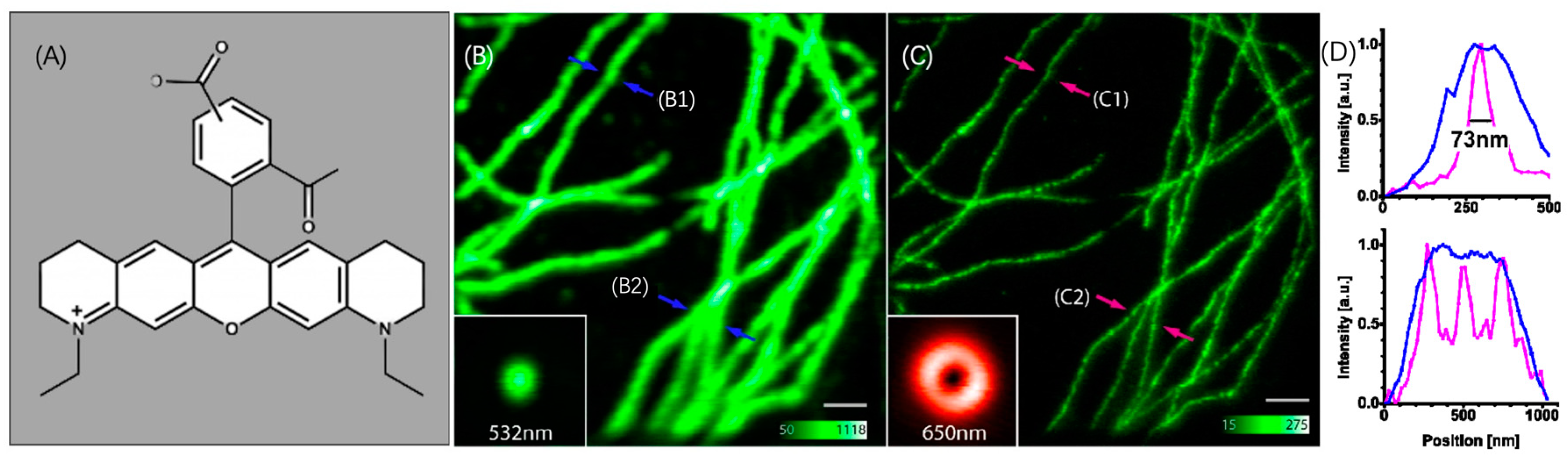
Figure 2.
(A)The structure of Rhodamine B. An- indicates anion. (B) The structure of ATTO 532. (C) The structural switching of ATTO 565 in different conditions[9].
Figure 2.
(A)The structure of Rhodamine B. An- indicates anion. (B) The structure of ATTO 532. (C) The structural switching of ATTO 565 in different conditions[9].
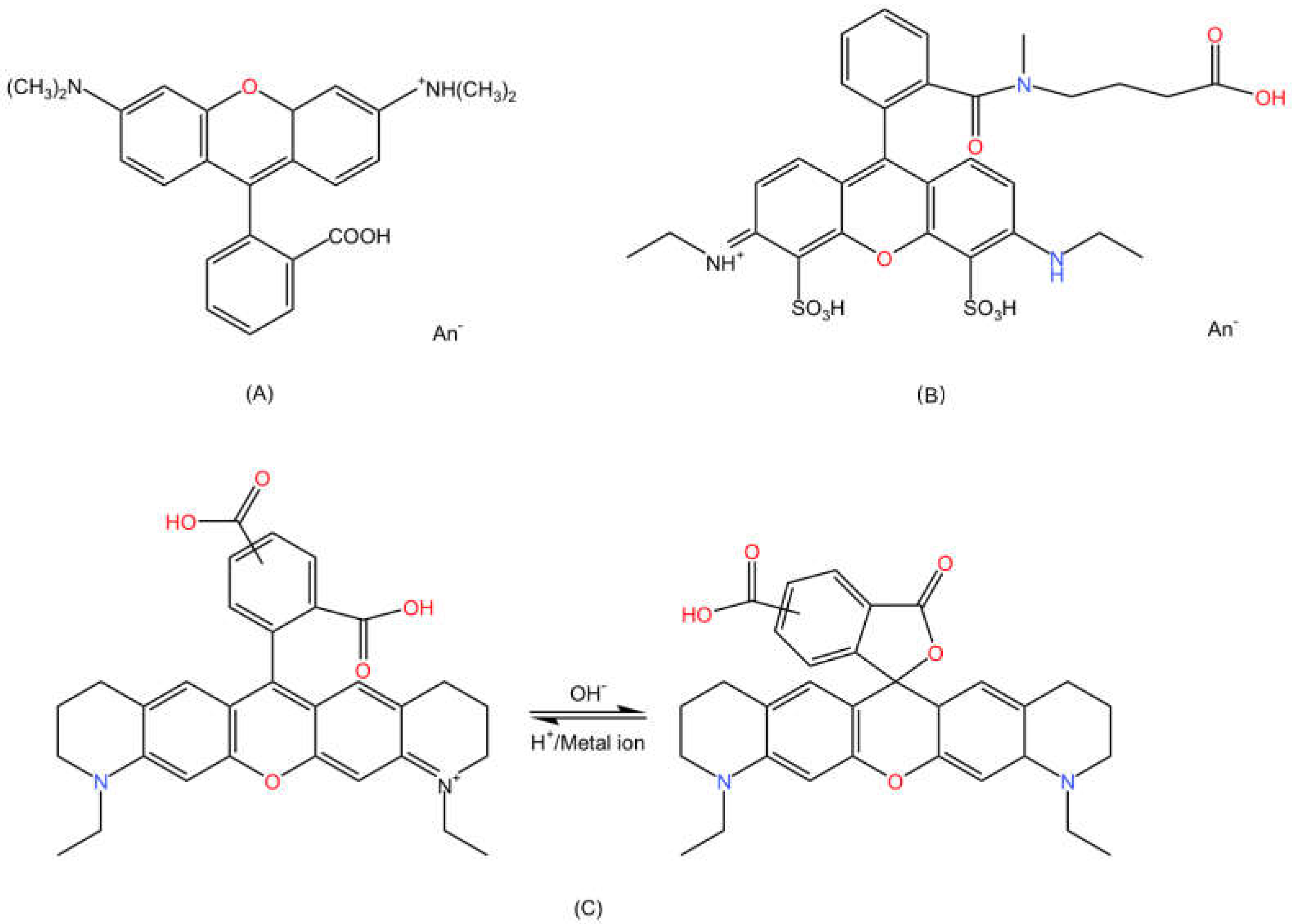
Figure 3.
(A) The absorption and fluorescence spectrum of ATTO 565 [12]. (B) Fluorescence time trace of a single molecule of dye ATTO 565. Several dark states could be found before the molecule was photobleached. (C) Specific fluorescence intensity trace of (B) from 28.4 to 29.4 s which shows intermittency. Reprinted (adapted) with permission from Yeow, E.K.L.; Melnikov, S.M.; Bell, T.D.M.; De Schryver, F.C.; Hofkens, J. Characterizing the Fluorescence Intermittency and Photobleaching Kinetics of Dye Molecules Immobilized on a Glass Surface. J. Phys. Chem. A 2006, 110, 1726–1734, doi:10.1021/jp055496r. Copyright 2006 American Chemical Society [13].
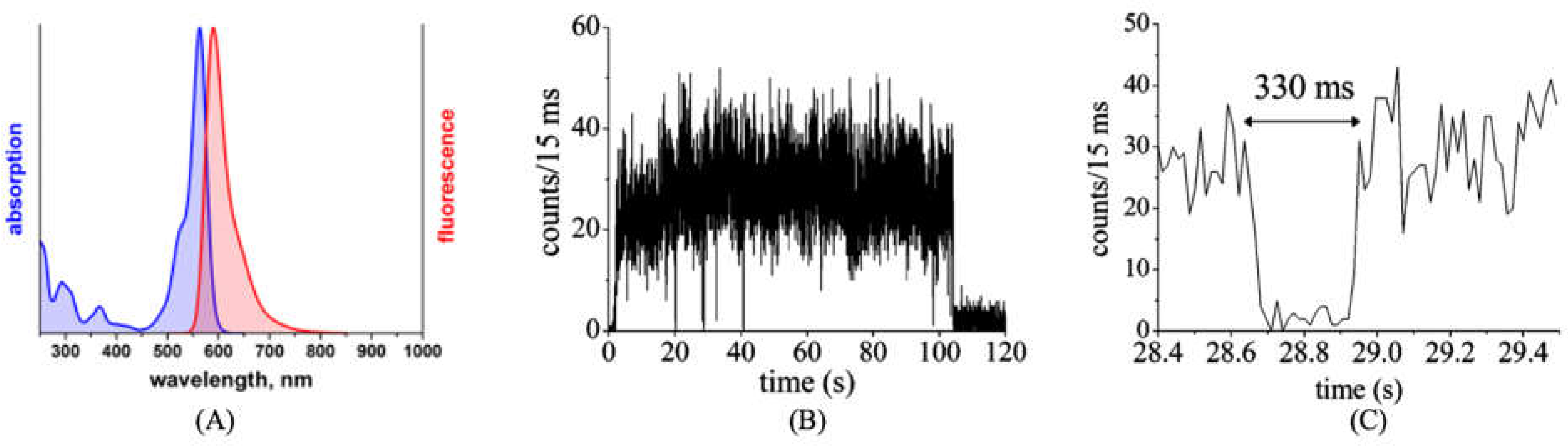
Figure 4.
Three electronic states are proposed as one of the explanations for blinking. S0 is the ground state. S1 is the first excited state. Molecule could go through radiative relaxation and go back to S0 from S1 with the emission of fluorescence. Refer to the end of the review for meanings of other symbols. The molecule could also go through the intersystem crossing and go to the first triplet excited state T1 state then relax to S0 without any fluorescence which implies the dark state. Reprinted (adapted) with permission from Yip, W.-T.; Hu, D.; Yu, J.; Vanden Bout, D.A.; Barbara, P.F. Classifying the Photophysical Dynamics of Single- and Multiple-Chromophoric Molecules by Single Molecule Spectroscopy. J. Phys. Chem. A 1998, 102, 7564–7575, doi:10.1021/jp981808x. Copyright 1998 American Chemical Society. [14].
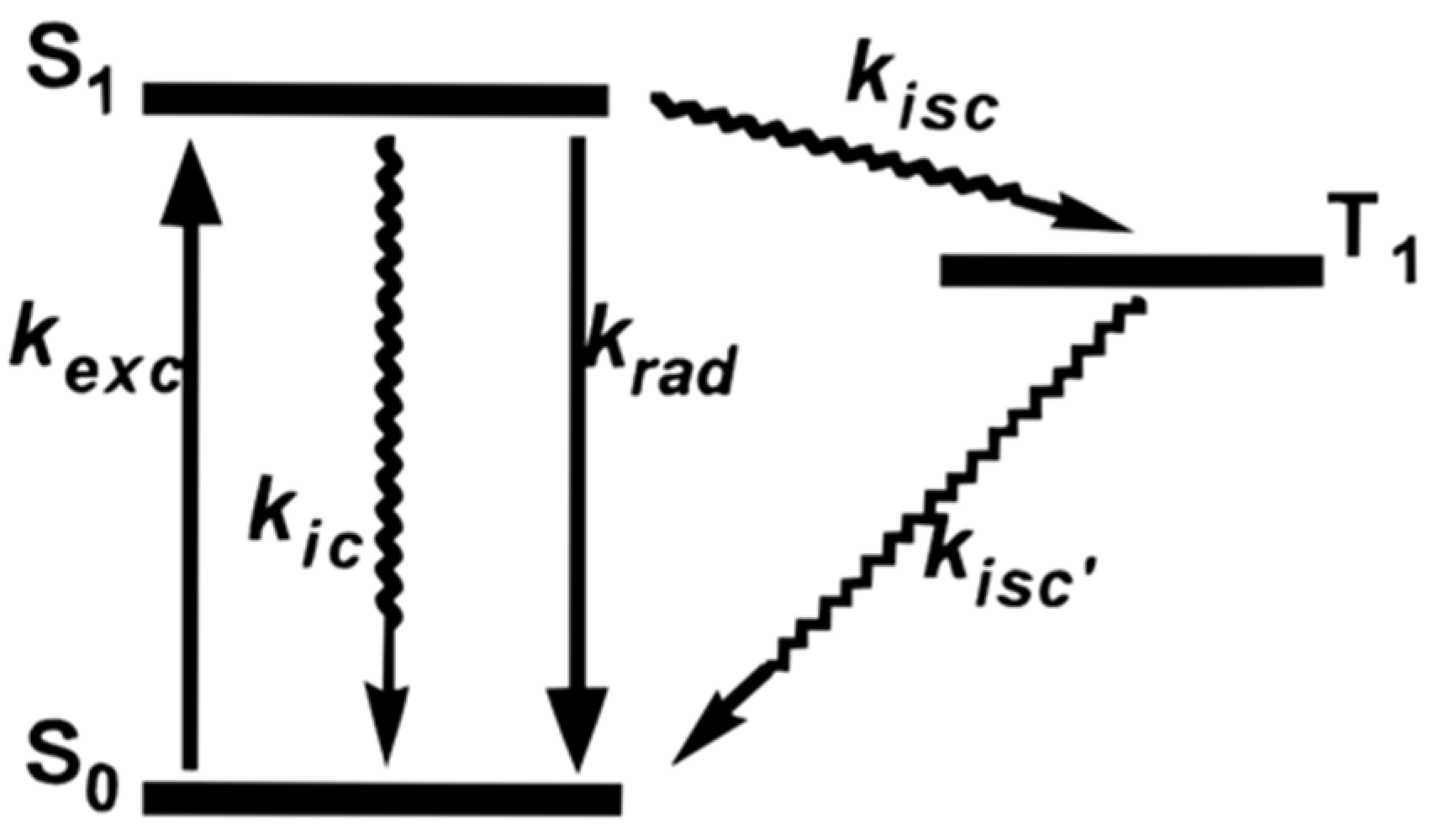
Figure 5.
Simulation diagram of the autocorrelation function of the fluorescence signal of fluorescent molecules.
Figure 5.
Simulation diagram of the autocorrelation function of the fluorescence signal of fluorescent molecules.
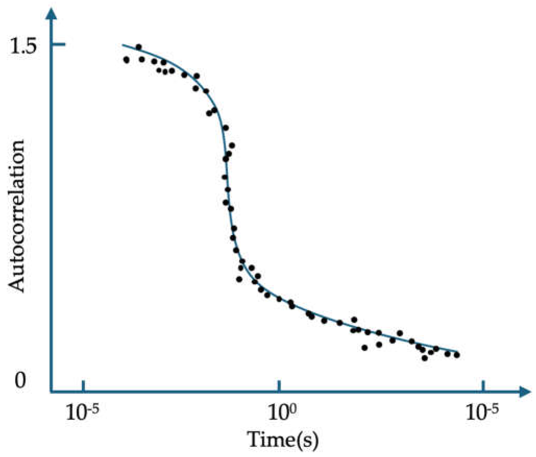
Figure 6.
Four electronic states explain the blinking phenomenon. Refer to the end of the document for meanings of other symbols. Reprinted (adapted) with permission from Yeow, E.K.L.; Melnikov, S.M.; Bell, T.D.M.; De Schryver, F.C.; Hofkens, J. Characterizing the Fluorescence Intermittency and Photobleaching Kinetics of Dye Molecules Immobilized on a Glass Surface. J. Phys. Chem. A 2006, 110, 1726–1734, doi:10.1021/jp055496r. Copyright 2006 American Chemical Society[13].
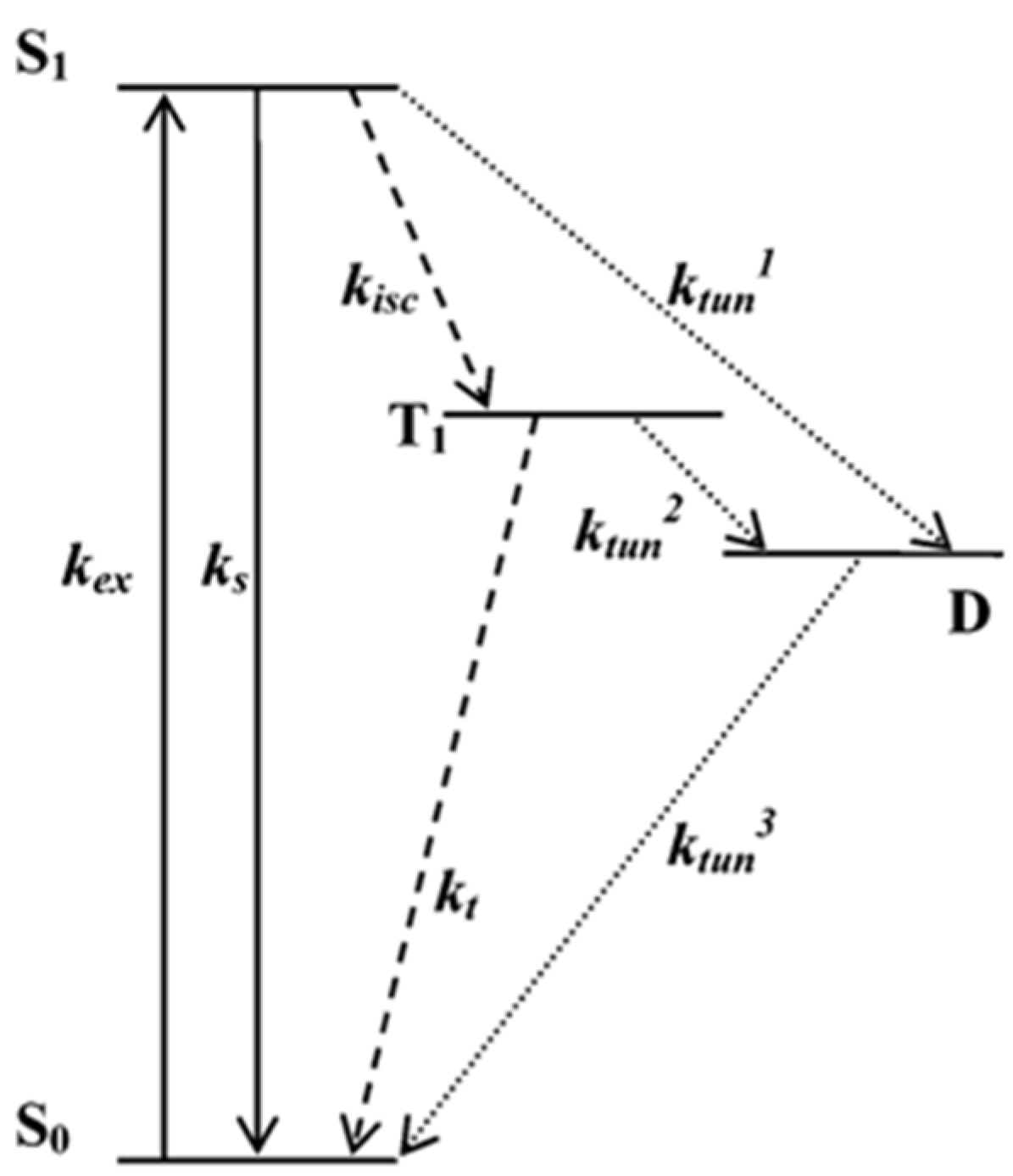
Figure 7.
ATTO 565 molecules were put into the lighting of different intensities. (A) 1136 W/cm2, (B) 568 W/cm2, (A) 284 W/cm2, the average bleaching times are 18.2 s (A), 21.8 s (B), and 63.0 s (C). Reprinted (adapted) with permission from Yeow, E.K.L.; Melnikov, S.M.; Bell, T.D.M.; De Schryver, F.C.; Hofkens, J. Characterizing the Fluorescence Intermittency and Photobleaching Kinetics of Dye Molecules Immobilized on a Glass Surface. J. Phys. Chem. A 2006, 110, 1726–1734, doi:10.1021/jp055496r. Copyright 2006 American Chemical Society [13].
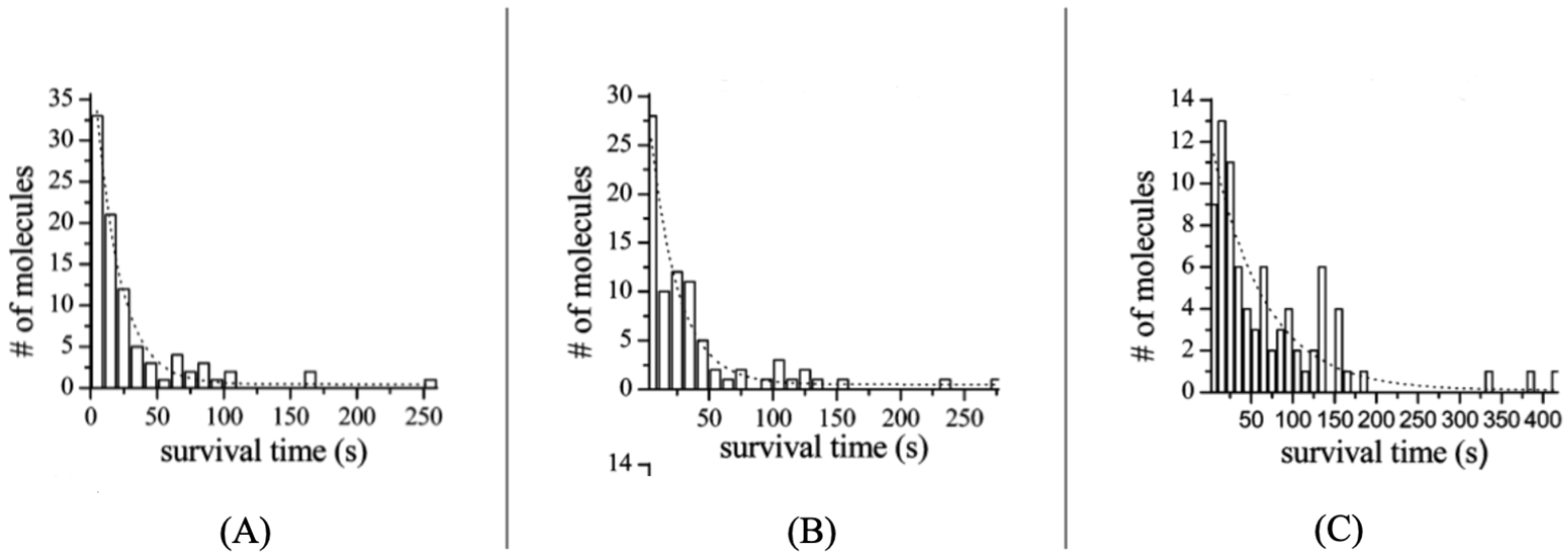
Figure 8.
(A) Temporal intensity profile of ATTO 565 photobleaching. A and B exhibit a trend of monoexponentially decay and C is biexponential decay. k1 = 5.1 × 10⁻⁴ s-1 and k2 = 2.9 × 10⁻³ s-1 for A. k3 = 2.2 × 10⁻³ s-1 and k4 = 1.2 × 10⁻² s-1 for B. k5 = 8.5 × 10⁻⁴ s-1 for C. (B) Energy-level diagram used to explain photobleaching. D is the radical state and B is the bleached state. Refer to the end of the document for meanings of other symbols. Reprinted (adapted) with permission from Yeow, E.K.L.; Melnikov, S.M.; Bell, T.D.M.; De Schryver, F.C.; Hofkens, J. Characterizing the Fluorescence Intermittency and Photobleaching Kinetics of Dye Molecules Immobilized on a Glass Surface. J. Phys. Chem. A 2006, 110, 1726–1734, doi:10.1021/jp055496r. Copyright 2006 American Chemical Society[13].
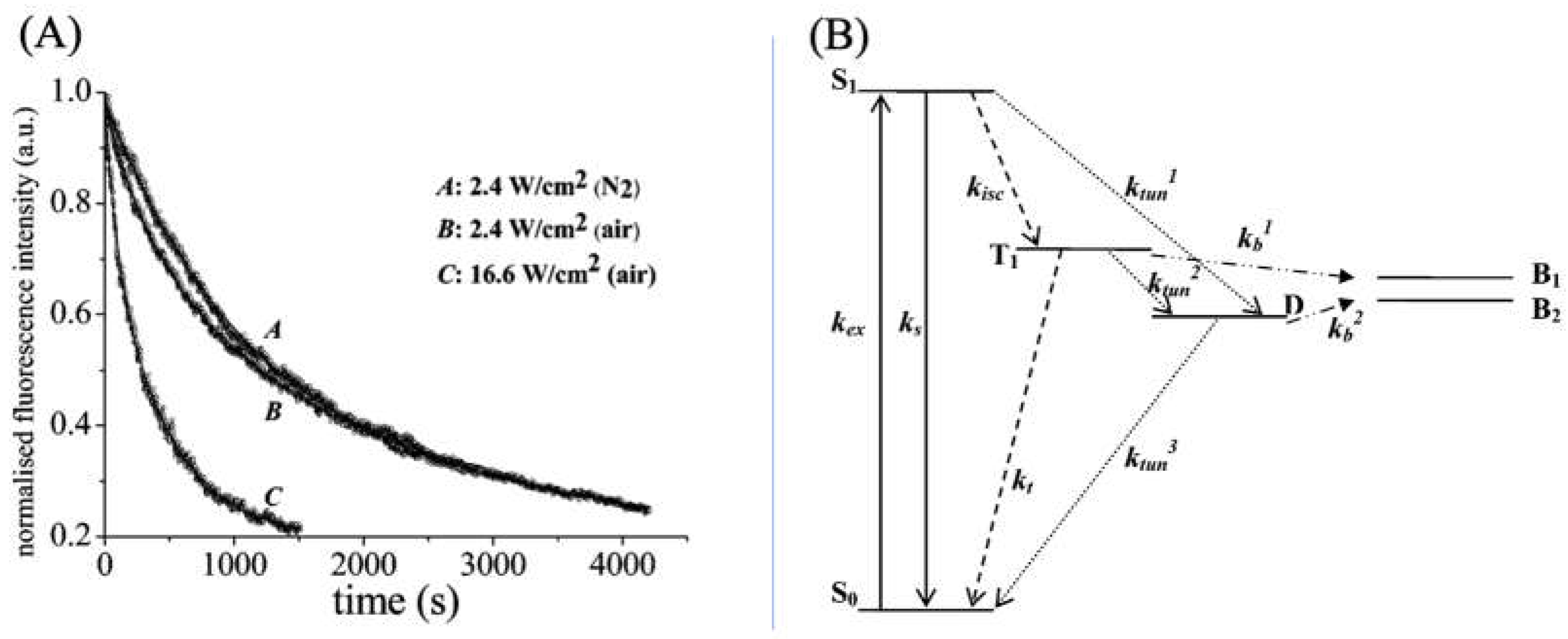
Figure 9.
(A) The SEM image of the nanochannel. (B) The confocal microscope image of the nanochannel. The fluorescence of ATTO 565 in red demonstrates the connectivity of microchannels. The diameter of the pipeline is 100 nanometers. Reprinted (adapted) with permission from Wang, L.P.; Shao, P.G.; van Kan, J.A.; Ansari, K.; Bettiol, A.A.; Pan, X.T.; Wohland, T.; Watt, F. Fabrication of Nanofluidic Devices Utilizing Proton Beam Writing and Thermal Bonding Techniques. Nucl. Instrum. Methods Phys. Res. Sect. B Beam Interact. Mater. At. 2007, 260, 450–454, doi:10.1016/j.nimb.2007.02.062. Copyright 2007 Elsevier B.V.[17].
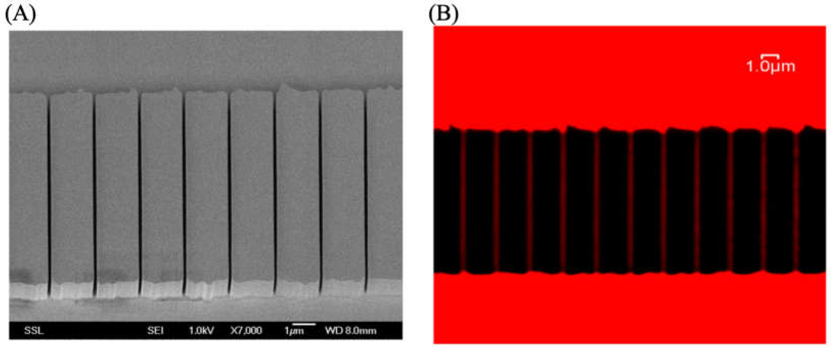
Figure 10.
(A) Cover the cell membrane inside-out on agarose beads using stir and wash. WGA on the beads immobilizes the cell membrane. (B) Confocal microscope image of Gαβγ-ATTO 565 on the beads. (C) Confocal microscope image of APEC-ATTO 633 on the beads. Scale bars of (B) and (C) are 20 μm (D) Shows the time-responsive fluorescence curve.Black circle curve illustrates the binding level of APEC to GPCR over time. The hollow circle curve illustrates the dynamic binding of APEC and GPCR in the presence of buffer. The black triangle curve shows the binding of Gαβγ and GPCR indicated by ATTO565 fluorescence. Reprinted (adapted) with permission from Roizard, S.; Danelon, C.; Hassaïne, G.; Piguet, J.; Schulze, K.; Hovius, R.; Tampé, R.; Vogel, H. Activation of G-Protein-Coupled Receptors in Cell-Derived Plasma Membranes Supported on Porous Beads. J. Am. Chem. Soc. 2011, 133, 16868–16874, doi:10.1021/ja205302g. Copyright 2011 American Chemical Society. [19].
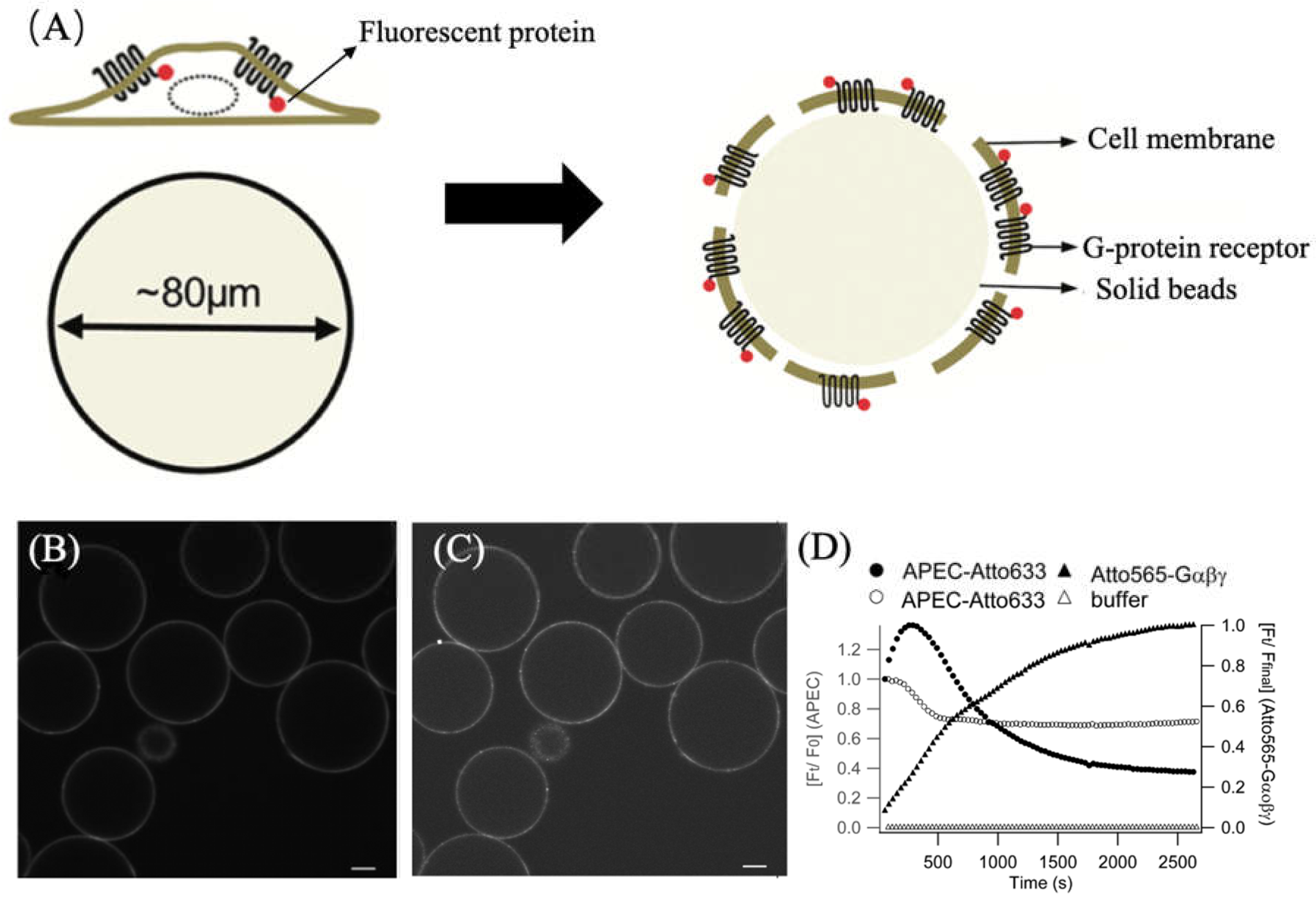
Figure 11.
(A) The SEM image of HA pores. The diameters of pores are ranged from 1 μm to 400 μm. The subfigure shows the tiniest pores with about 1 μm diameter. (B) The chemical structure of Rhodamine-phalloidin. These two molecules are conjugated by a thiourea. (C) These three images demonstrate the capability of ATTO565 to localize HOS cells at different depths in space from 10 μm to 32 μm. Reprinted (adapted) with permission from Cicuéndez, M.; Izquierdo-Barba, I.; Sánchez-Salcedo, S.; Vila, M.; Vallet-Regí, M. Biological Performance of Hydroxyapatite–Biopolymer Foams: In Vitro Cell Response. Acta Biomater. 2012, 8, 802–810, doi:10.1016/j.actbio.2011.09.019. Copyright 2011 Acta Materialia Inc [24].

Figure 12.
The confocal microscope images of F-actin. The red emission light comes from ATTO 565-phalloidin-F-actin and green emission light comes from GFP-dysferlin-caveolin. The number marked in the lower left corner is the Z value, which represents the depth of the focal plane. Used with permission of Marg, A.; Schoewel, V.; Timmel, T.; Schulze, A.; Shah, C.; Daumke, O.; Spuler, S. Traffic 2012, 13, 1286–1294; permission conveyed through Copyright Clearance Center, Inc [28].
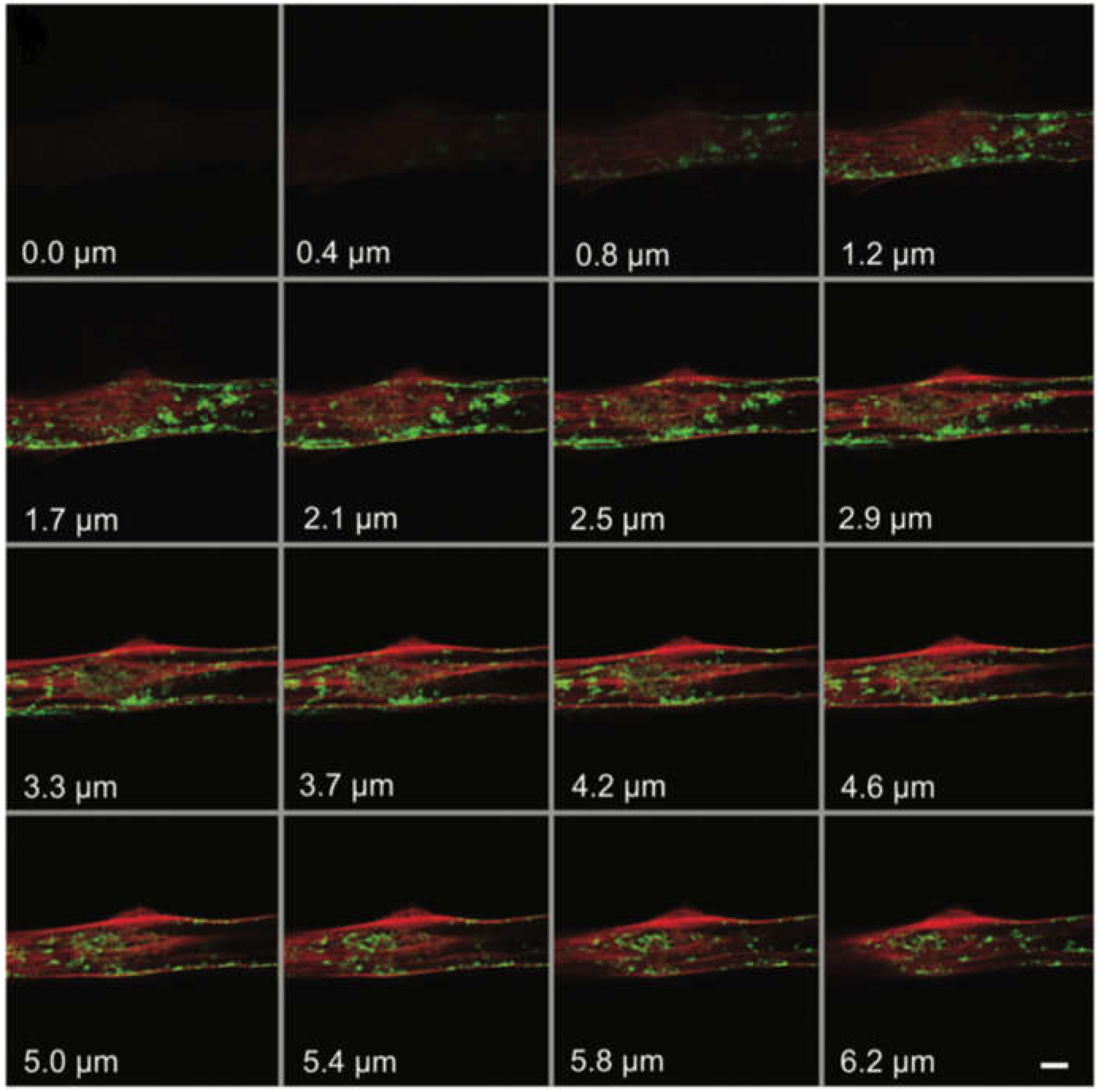
Figure 13.
The confocal and STED microscope image of syntaxin-GFP. Low, medium and high indicate the fluorescent protein expression level. (A, B) The confocal images. Membrane sheets showing highly variable syntaxin levels were distinguishable by their staining intensities and were occasionally found within the same field of view.(C, D) In STED mode, photos taken at the same location show significantly improved resolution. Reprinted from Biophysical Journal, Vol 90, Jochen J. Sieber, Katrin I. Willig,y Rainer Heintzmann,z Stefan W. Hell,y and Thorsten Lang, The SNARE Motif Is Essential for the Formation of Syntaxin Clusters in the Plasma Membrane, 2843-2851, Copyright (2006), with permission from Elsevier [34].
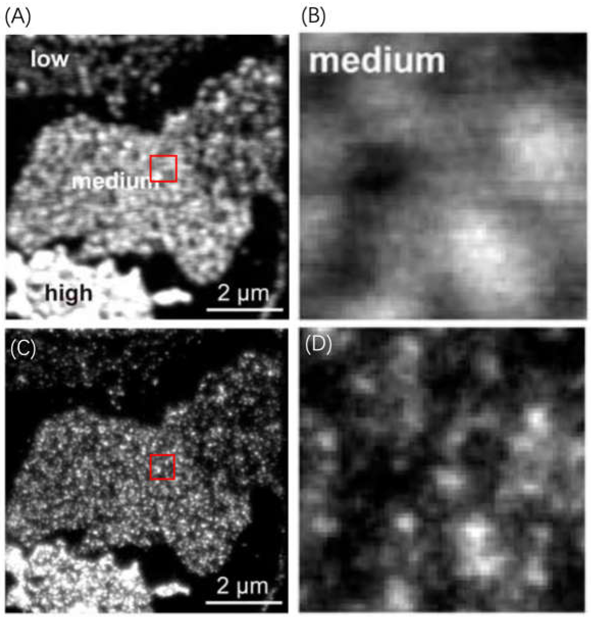
Figure 14.
Variation of bleaching efficiency β with STED light intensity at different pulse durations. In the same time intervals, the extent of dye bleaching increases with the increasing intensity of STED red light. Reprinted with permission from Dyba, M.; Stefan, H. Photostability of a Fluorescent Marker under Pulsed Excited-State Depletion through Stimulated Emission. Appl. Opt. 2003, 42, 5123, doi:10.1364/AO.42.005123 © Optical Society of America[36].
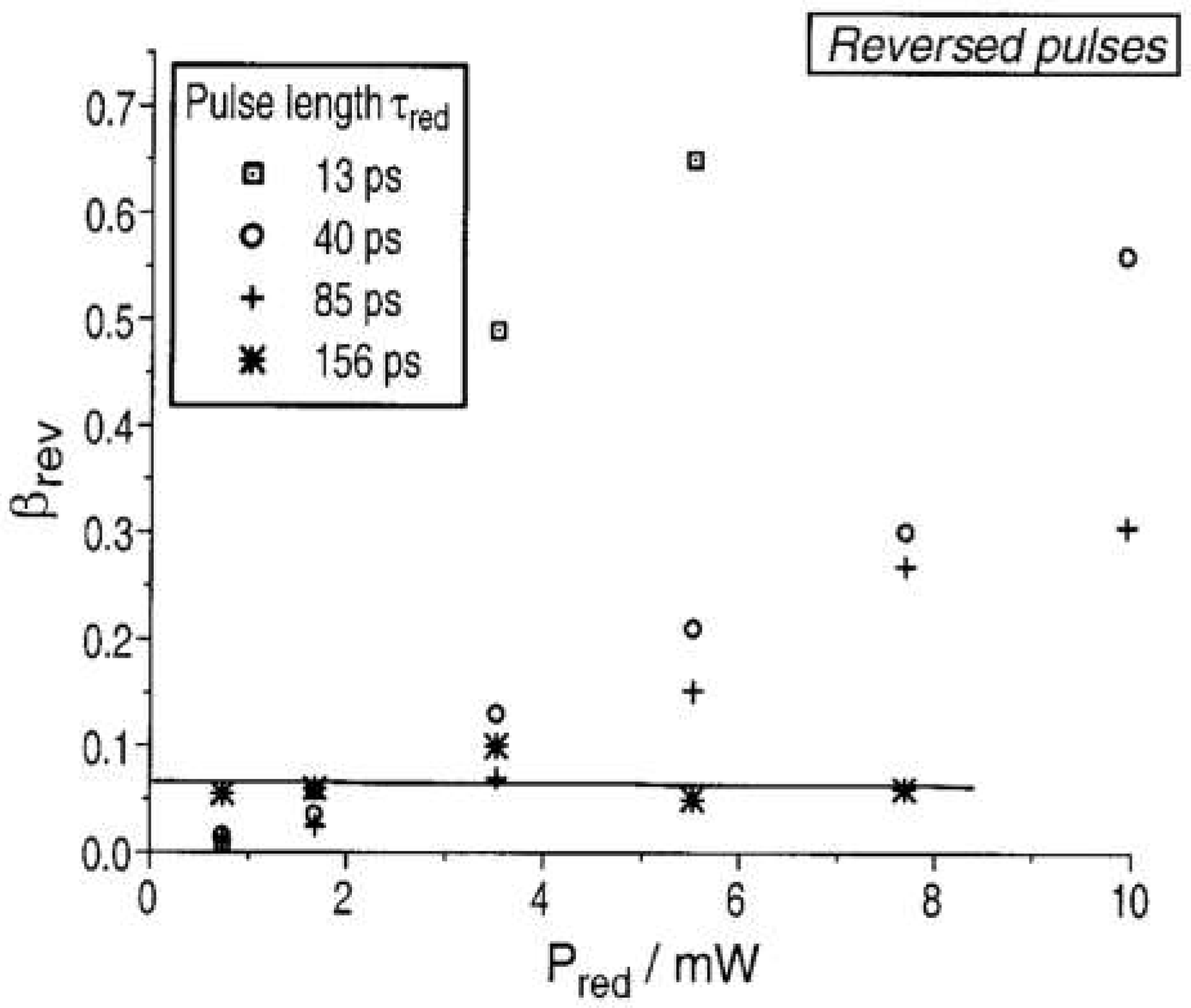
Figure 15.
(A) The image of the tubular fibers was obtained with a confocal microscope. (B) The image of the same tubular fibers was scanned with a STED microscope. (C) The line graphs show the FWHM at the arrow location. Upper image for A1 and lower image for A2. Scale bar: 1 μm. Reprinted/Adapted with permission from Wildanger, D.; Rittweger, E.; Kastrup, L.; Hell, S.W. STED Microscopy with a Supercontinuum Laser Source. Opt. Express 2008, 16, 9614–9621, doi:10.1364/OE.16.009614 © Optical Society of America [5].
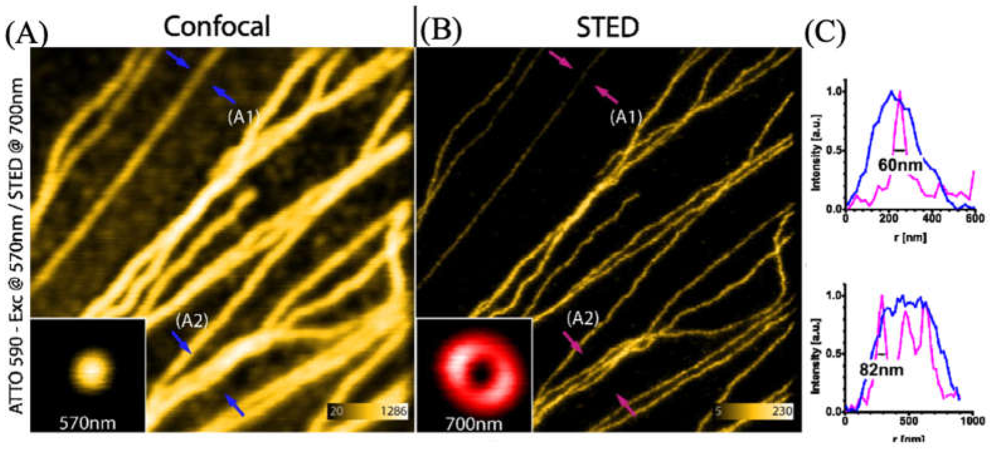
Figure 16.
The structure of trisNTA-OEG-fluorophores. Reprinted (adapted) with permission from Lata, S.; Gavutis, M.; Tampé, R.; Piehler, J. Specific and Stable Fluorescence Labeling of Histidine-Tagged Proteins for Dissecting Multi-Protein Complex Formation. J. Am. Chem. Soc. 2006, 128, 2365–2372, doi:10.1021/ja0563105. Copyright 2006 American Chemical Society [38]. The fluorophore could be any kind of rhodamine dye.
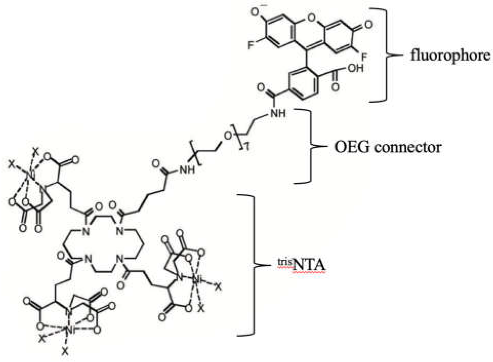
Figure 17.
(A) Image of Sf9 cells stained by FEW646tris-NTA. (B) The fluorescent dye is washed away after incubation in 100 mM imidazole, indicating the reversible stain. On the left side are the confocal fluorescent images, and on the right side are the transmission images of Sf9 cells. Reprinted (adapted) with permission from Lata, S.; Gavutis, M.; Tampé, R.; Piehler, J. Specific and Stable Fluorescence Labeling of Histidine-Tagged Proteins for Dissecting Multi-Protein Complex Formation. J. Am. Chem. Soc. 2006, 128, 2365–2372, doi:10.1021/ja0563105. Copyright 2006 American Chemical Society [38].
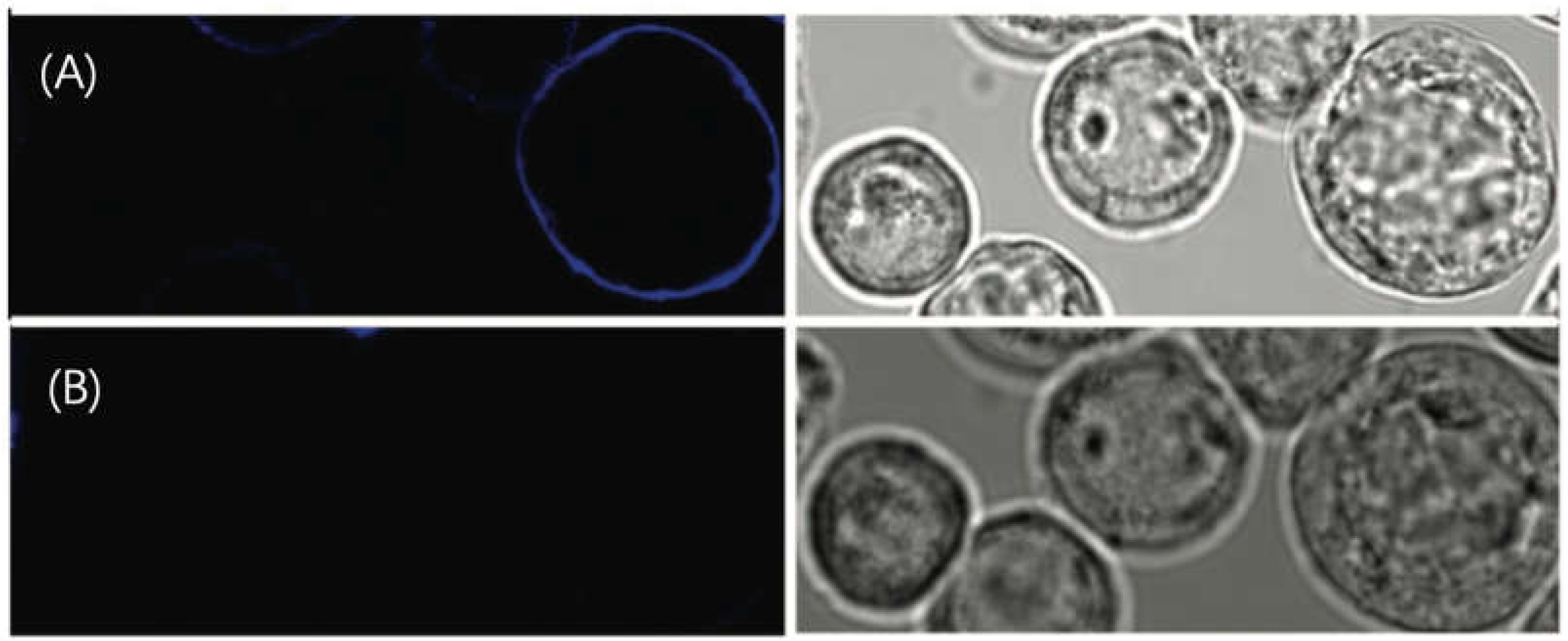
Figure 18.
(a) The structure of trisNTA-PPII-ATTO 565. X indicates the monomer number of PPII. (b) The fluorescence spectrum shows the fluorescence intensity is positively correlated with the connector length. (c) The fluorescence spectrum indicates that when the monomer number reaches 8, the fluorescence intensity is essentially equivalent to that of the free fluorophore. Reprinted (adapted) with permission from Grunwald, C.; Schulze, K.; Giannone, G.; Cognet, L.; Lounis, B.; Choquet, D.; Tampé, R. Quantum-Yield-Optimized Fluorophores for Site-Specific Labeling and Super-Resolution Imaging. J. Am. Chem. Soc. 2011, 133, 8090–8093, doi:10.1021/ja200967z. Copyright 2011 American Chemical Society. [39].
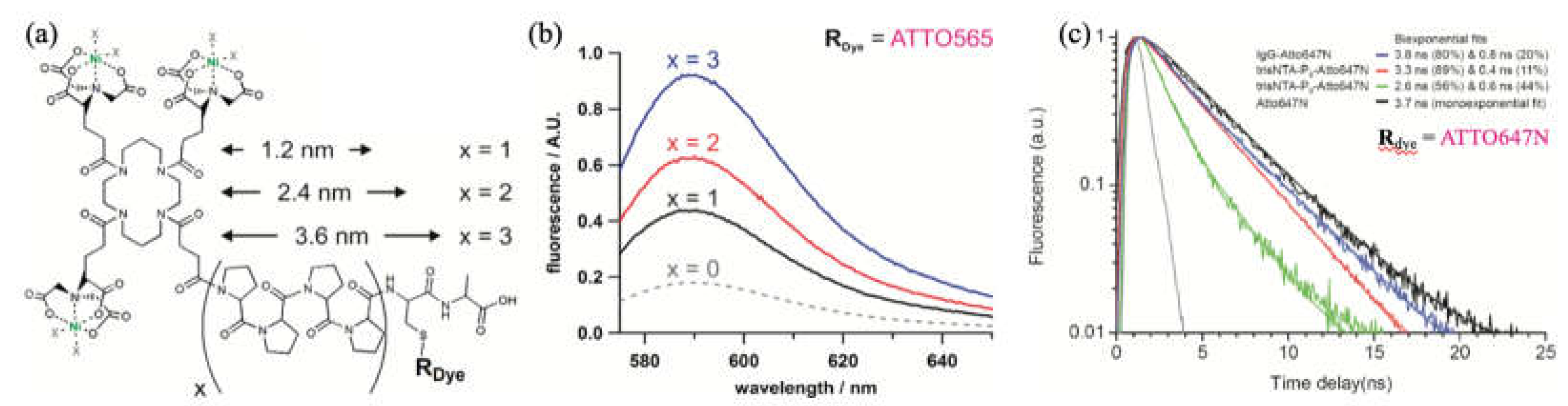
Figure 19.
(A) A scheme of an individual fluorescent signal emitted by a single molecule. The intensity in the middle is the highest, which indicates the location of the molecule. (B) A scheme shows the distribution of intensity in one signal. Reprinted (adapted) with permission from Von Diezmann, L.; Shechtman, Y.; Moerner, W.E. Three-Dimensional Localization of Single Molecules for Super-Resolution Imaging and Single-Particle Tracking. Chem. Rev. 2017, 117, 7244–7275, doi:10.1021/acs.chemrev.6b00629. Copyright 2017 American Chemical Society[46].
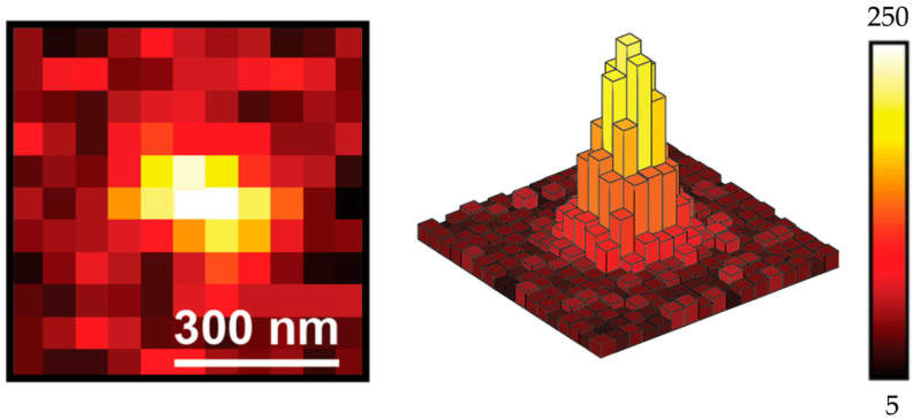
Figure 20.
(A) The scheme of transportation and assembling of Env in the target cell. The green object is Env and it’s finally confined at the Gap. (B, C) The result of the SMT. The displacement of WT-Env is smaller than others, indicating that the assembling of CTΔ144-Env-ATTO 565 and d8-Env-ATTO 565 on the Gap is obstructed. Reprinted (adapted) with permission from Buttler, C.A.; Pezeshkian, N.; Fernandez, M.V.; Aaron, J.; Norman, S.; Freed, E.O.; Van Engelenburg, S.B. Single Molecule Fate of HIV-1 Envelope Reveals Late-Stage Viral Lattice Incorporation. Nat. Commun. 2018, 9, 1861, doi:10.1038/s41467-018-04220-w. Copyright 2018, Carmen A. Buttler [51].
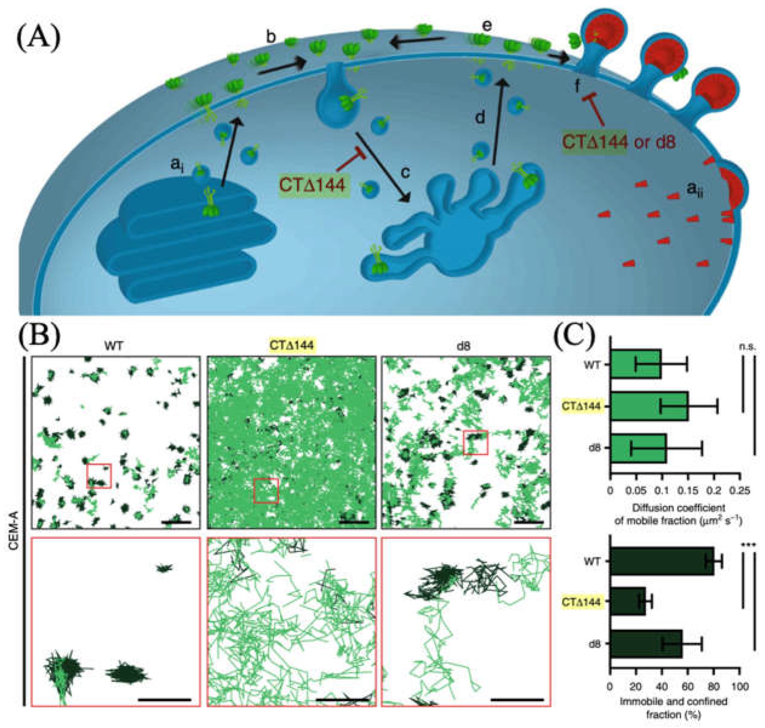
Figure 21.
(A) CL has focus a for the Y-axis and focus b for the X-axis. On the other side, it has focus planes A, B, and C. (B) The image of the red fluorescent latex bead with and without a CL. Reprinted (adapted) with permission from Kao, H.P.; Verkman, A.S. Tracking of Single Fluorescent Particles in Three Dimensions: Use of Cylindrical Optics to Encode Particle Position. Biophys. J. 1994, 67, 1291–1300, doi:10.1016/S0006-3495(94)80601-0. Copyright 1994 The Biophysical Society [53].
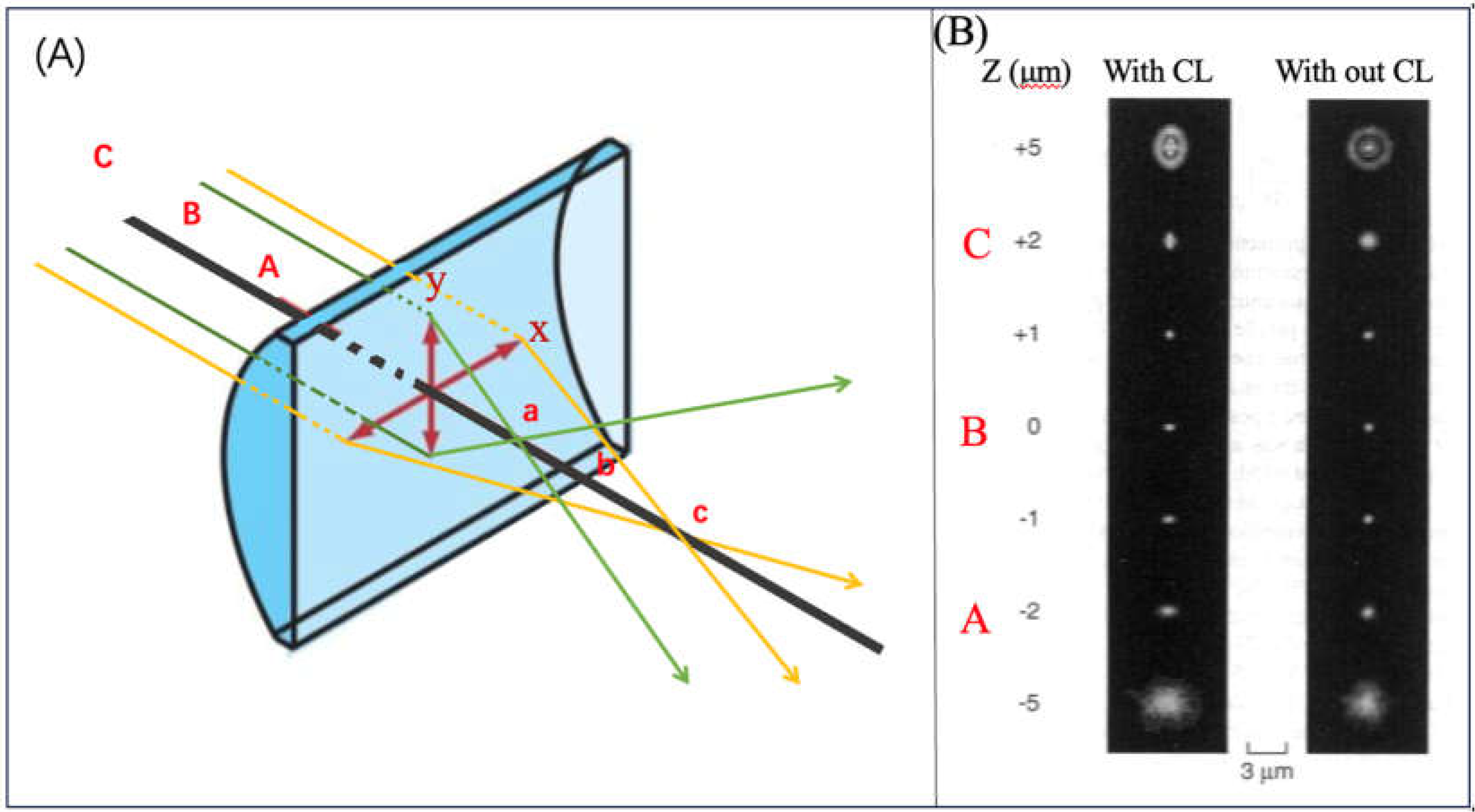
Figure 22.
(A) Fluorescent schematic diagram of a single molecular at a certain height. The shape follows a 2D Gaussian elliptical distribution. The scale in this context measures the photon density. (B) The scatter plot and calibration curve of PSF and Z values.
Figure 22.
(A) Fluorescent schematic diagram of a single molecular at a certain height. The shape follows a 2D Gaussian elliptical distribution. The scale in this context measures the photon density. (B) The scatter plot and calibration curve of PSF and Z values.
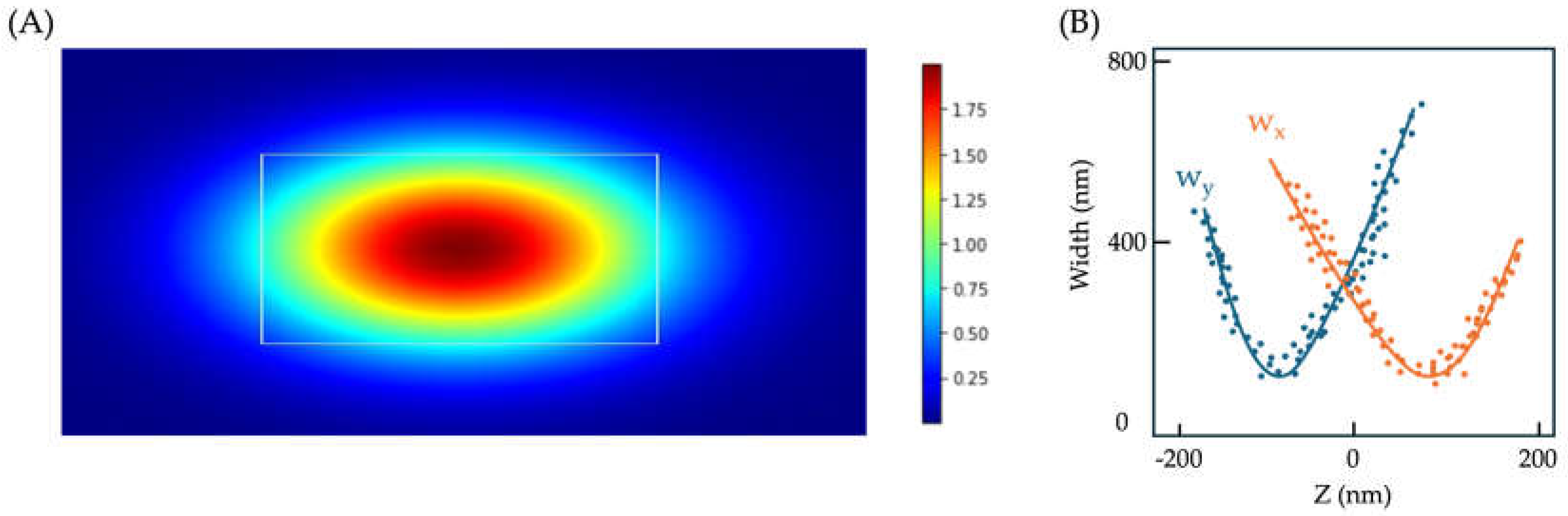
Figure 23.
A) The scheme shows the biggest difference between the LSM and traditional micro-scope. The light passes through the sample and doesn't directly go into the eyepiece. (B) Diagram of space constraint. (C) The LSM system used by Li et al. Reprinted (adapted) with permission from Li, Y.; Hu, Y.; Cang, H. Light Sheet Microscopy for Tracking Single Molecules on the Apical Surface of Living Cells. J. Phys. Chem. B 2013, 117, 15503–15511, doi:10.1021/jp405380g. Copyright 2013 American Chemical Society [47].
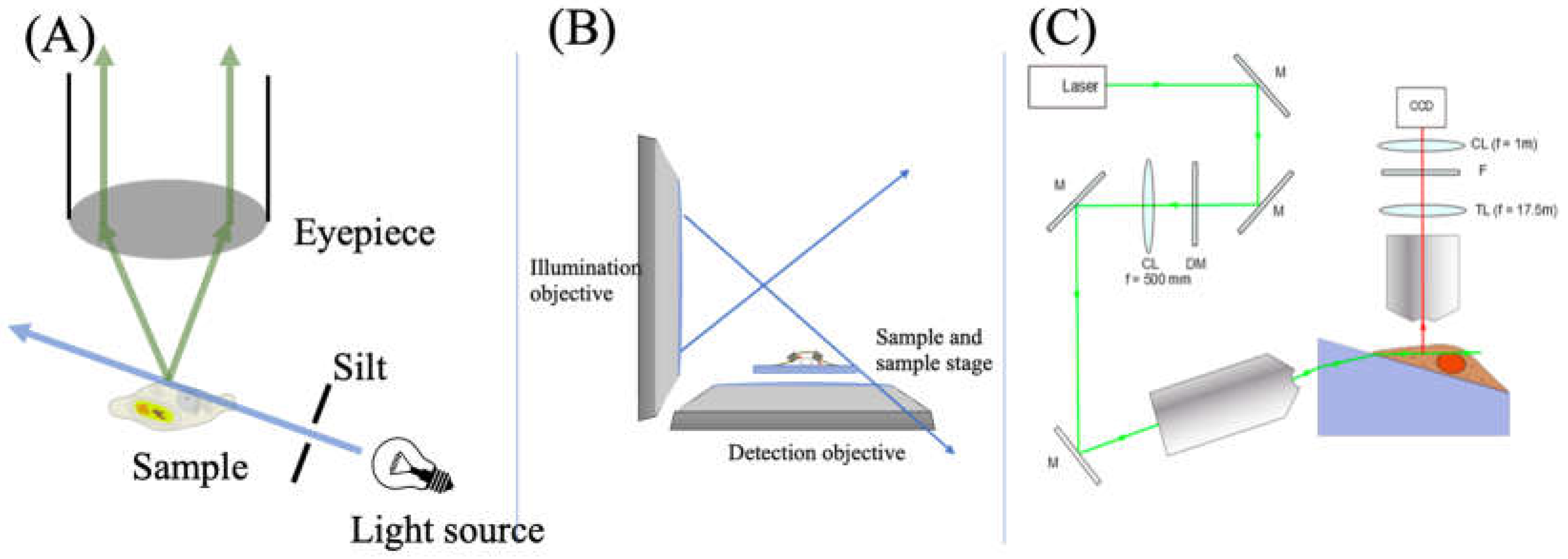
Figure 24.
The calibration curve was measured by fluorescent beads and LSM. The image exhibits varying degrees of ellipticity at different distances from the focal plane. Reprinted (adapted) with permission from Li, Y.; Hu, Y.; Cang, H. Light Sheet Microscopy for Tracking Single Molecules on the Apical Surface of Living Cells. J. Phys. Chem. B 2013, 117, 15503–15511, doi:10.1021/jp405380g. Copyright 2013 American Chemical Society [47].
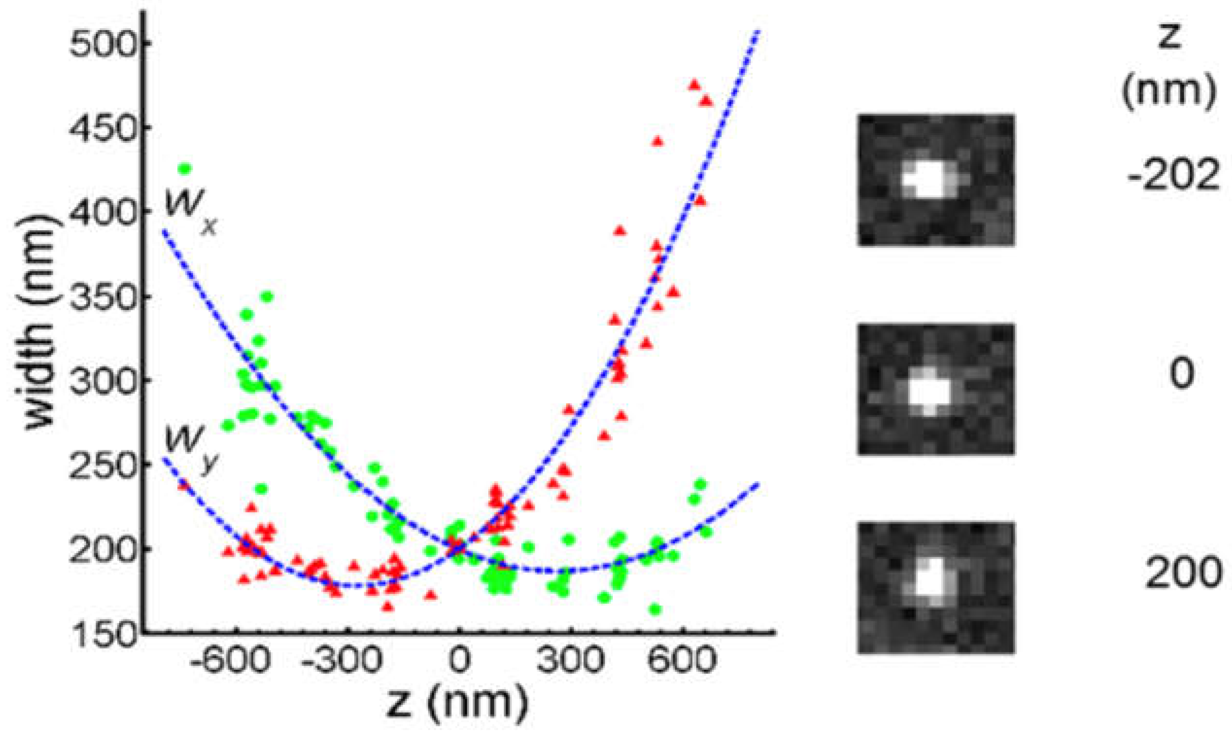
Figure 25.
A) The 2D image was shot by the LSM. The molecule went into the ROI at -0.02 s and out or photobleached at 1.28 s. (B) The 3D visualized trajectory of the molecule from 0 s to 8 s. After 8 s, the molecule is too deviaed to simulate the trail. Reprinted (adapted) with permission from Li, Y.; Hu, Y.; Cang, H. Light Sheet Microscopy for Tracking Single Molecules on the Apical Surface of Living Cells. J. Phys. Chem. B 2013, 117, 15503–15511, doi:10.1021/jp405380g. Copyright 2013 American Chemical Society [47].
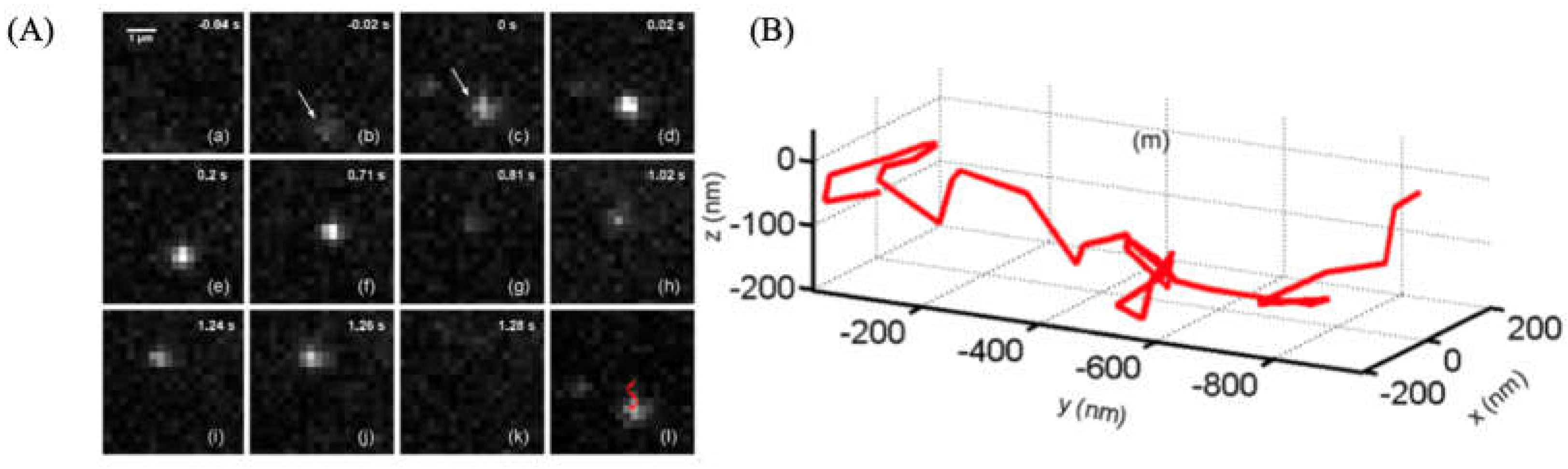
Figure 26.
(A, C) The intensity-time line graph of the periodical signal and the noise. (B, D) The ACF of the signal and the noise.
Figure 26.
(A, C) The intensity-time line graph of the periodical signal and the noise. (B, D) The ACF of the signal and the noise.
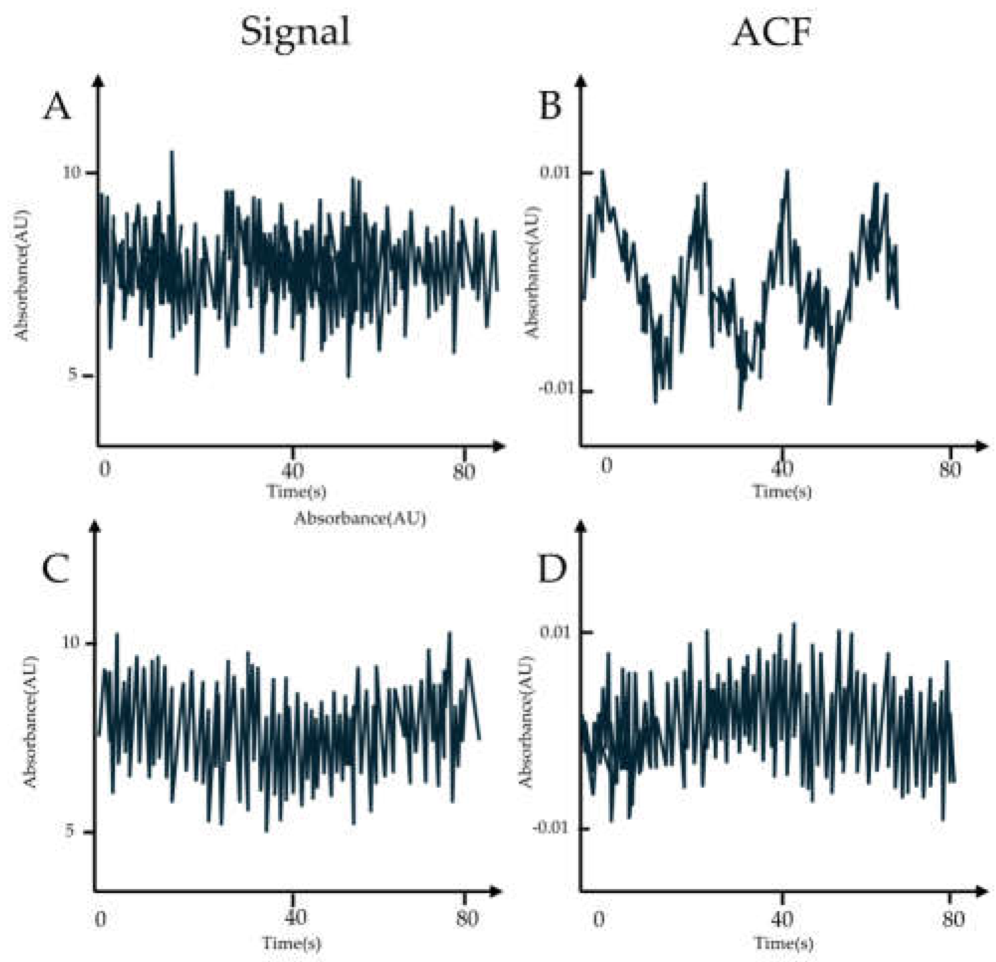
Figure 27.
The chemical reaction equation for the hypothetical alteration of ATTO 565's structure to make it responsive to metal ions. Reprinted (adapted) with permission from Kim, H.N.; Lee, M.H.; Kim, H.J.; Kim, J.S.; Yoon, J. A New Trend in Rhodamine-Based Chemosensors: Application of Spirolactam Ring-Opening to Sensing Ions. Chem. Soc. Rev. 2008, 37, 1465, doi:10.1039/b802497a. Permission conveyed through Copyright Clearance Center, Inc.
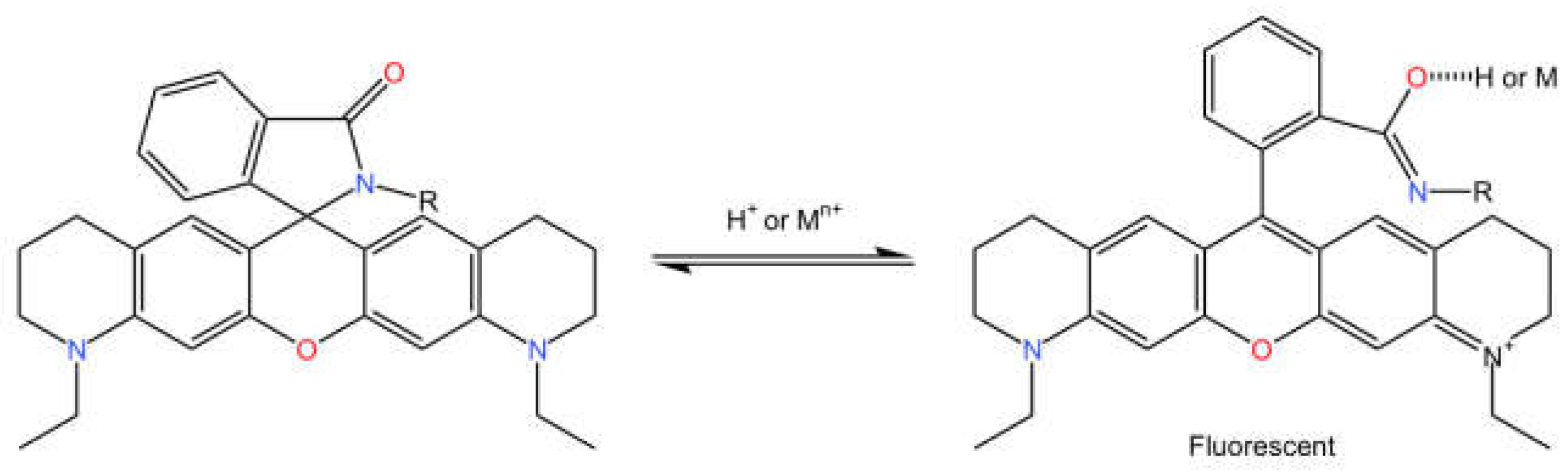

Table 1.
The optical data of ATTO 565 [12].
Table 1.
The optical data of ATTO 565 [12].
| λabs (nm) | 564 |
| εmax (M-1cm-1) | 1.2 × 10⁵ |
| λfl (nm) | 590 |
| Φfl (%) | 90 |
| τfl (ns) | 4.0 |
Table 2.
The cost matrix.
| Cost matrix | Frame t+1 | ||||||||
| Linking | No Linking | ||||||||
| 1 | 2 | 3 | 4 | I | II | III | |||
| Frame t | Linking | I | lI1 | lI2 | X | X | d | X | X |
| II | LII1 | LII2 | LII3 | LII4 | X | d | X | ||
| III | X | LIII2 | LIII3 | LIII4 | X | X | d | ||
| No linking | 1 | b | X | X | X | ||||
| 2 | X | b | X | X | |||||
| 3 | X | X | b | X | |||||
| 4 | X | X | X | b | |||||
Table 3.
An example of the assignment matrix.
| Assignment matrix | Frame t+1 | ||||||||
| Linking | No Linking | ||||||||
| 1 | 2 | 3 | 4 | I | II | III | |||
| Frame t | Linking | I | 1 | 0 | 0 | 0 | 0 | 0 | 0 |
| II | 0 | 0 | 0 | 0 | 0 | 1 | 0 | ||
| III | 0 | 0 | 0 | 1 | 0 | 0 | 0 | ||
| No linking | 1 | 0 | 0 | 0 | 0 | 1 | 0 | 0 | |
| 2 | 0 | 1 | 0 | 0 | 0 | 0 | 0 | ||
| 3 | 0 | 0 | 1 | 0 | 0 | 0 | 0 | ||
| 4 | 0 | 0 | 0 | 0 | 0 | 0 | 1 | ||
Table 4.
The diffusion time of ATTO 565 in different concentration of AAc [59].
Table 4.
The diffusion time of ATTO 565 in different concentration of AAc [59].
| AAc concentration (%) | Diffusion time (s) |
| 0.25 | 4.51E-05 |
| 2.5 | 5.27E-05 |
| 5 | 5.76E-05 |
| 8 | 6.53E-05 |
| 9 | 7.12E-05 |
| 10 | 7.34E-05 |
Disclaimer/Publisher’s Note: The statements, opinions and data contained in all publications are solely those of the individual author(s) and contributor(s) and not of MDPI and/or the editor(s). MDPI and/or the editor(s) disclaim responsibility for any injury to people or property resulting from any ideas, methods, instructions or products referred to in the content. |
© 2024 by the authors. Licensee MDPI, Basel, Switzerland. This article is an open access article distributed under the terms and conditions of the Creative Commons Attribution (CC BY) license (https://creativecommons.org/licenses/by/4.0/).
Copyright: This open access article is published under a Creative Commons CC BY 4.0 license, which permit the free download, distribution, and reuse, provided that the author and preprint are cited in any reuse.


