
Submitted:
24 June 2024
Posted:
25 June 2024
You are already at the latest version
Abstract
The algorithm described in this paper inherits the concepts of layered fusion, insertion, and set from four convex hull-based heuristic algorithms. It summarizes relevant definitions and theorems, proposes valuable research hypotheses, combines grouping and insertion, and innovatively introduces the practice of "grouped insertion."
Keywords:
TSP
; Convex Hull
; Improved Algorithm
1. Introduction
Perhaps you had pondered its essence before ever hearing about the Traveling Salesman Problem, much like contemplating questions in childhood only to discover them written in philosophy textbooks later.
In this era of the fourth technological revolution, characterized by an information explosion, humanity utilizes computers, smartphones, tablets, forums, document repositories, video platforms, search engines, artificial intelligence, and data dashboards. In this digital age, the characters on the screen consistently affirm that the Traveling Salesman Problem holds great theoretical and practical significance. However, as people initially gazed up at the sky, they began to yearn for answers to intriguing questions like, “Why is the sky blue?” The vast river of literature rarely mentions that the Traveling Salesman Problem is also an intriguing question.
While “The Origin of the Blue Sky” has already responded to “Why is the sky blue?” the answer to the Traveling Salesman Problem remains shrouded in mist. Carrying the simplest of hopes, new algorithms for the Traveling Salesman Problem continue to grow like branches and emerge like leaves, reaching towards higher and bluer realms. In this sparsely populated branch of the tree, it is hoped that this text may sprout a new bud.
Our paper is organized as follows. First, we delve into the research background, including the history and current status of the Traveling Salesman Problem, as well as the development and current status of four convex hull-based heuristic algorithms. Second, we describe the algorithm itself, including definitions, theorems, hypotheses, concepts, and steps. Third, we conduct data testing.
2. Research StatuS
2.1. Traveling Salesman Problem Overview
In 1759, Leonhard Euler introduced the Knight’s Tour Problem, which involved visiting all 64 squares of a chessboard exactly once and returning to the starting point.
In 1859, the mathematician W.R. Hamilton proposed a game called “Around the World,” where famous cities like London, Paris, and Moscow were labeled on the 20 vertices of a regular dodecahedron. The objective was for the player to start from any city, visit all cities exactly once, and then return to the starting point.
In 1949, Robinson used the term “Traveling Salesman Problem” in a paper, making it the earliest known use of this term in the existing literature.
In 1954, George Bernard Dantzig and others made a historic breakthrough in the Traveling Salesman Problem using linear programming, solving it for 48 cities in the United States.
Today, the Traveling Salesman Problem is described as follows: A salesman needs to travel to multiple cities to sell products. Starting from one city, the salesman must visit all cities and return to the starting city. The challenge is to choose the route that minimizes the total distance traveled.
2.2. Heuristic Algorithms Based on Convex Hull
The following are descriptions of four heuristic algorithms based on the convex hull or related to the convex hull. For better narrative and understanding, the names used are directly from the referenced literature, while the concepts and technical terms are paraphrased.
Convex Hull Contraction Method: The primary idea is to construct a convex hull as the initial circuit and gradually insert the remaining points into the circuit one by one until no points remain. The insertion principle at each step is to minimize the length of the route after insertion [1]. This algorithm includes the professional term “increment,” defined in the text as S(i, j, k) = |ik| + |jk| - |ij|, where i and j are adjacent points on the visited route, and k is a point not on the visited route. This can be understood as the length of the route after the point is inserted minus the length before insertion. This algorithm combines the ideas of the convex hull and the minimum insertion method, making it a foundational approach among the four.
Convex Hull Working Set TSP Algorithm: The main idea is to treat all points as a set, calculate the convex hull, and determine the membership of each point by computing the degree of belonging to the remaining points. The working set is divided into new sets based on the edges of the convex hull. This process continues, dividing new working sets until each set contains only two points [2]. The term “membership” is included in this algorithm, defined as f(i, j, k) = 1 / (|ik| + |jk| - |ij|), where i and j are two vertices of the convex hull, and k belongs to the set of points within the maximum internal convex hull. This algorithm combines the ideas of the convex hull, minimum insertion method, and the divide-and-conquer approach. It differs from the Convex Hull Contraction Method in terms of the objects being inserted and involves more frequent use of the convex hull, making it a more complex algorithm.
TSP Construction Algorithm Based on a Hierarchical Model: The main idea involves two phases. In the first phase, a pseudo-convex hull operator is used to construct a hierarchical model. In the second phase, the obtained hierarchical model is fused from the innermost layer to the outermost layer following fusion rules. The fusion rule starts from the innermost layer, randomly selects points from the relatively outer layer, and inserts them one by one into the circuit until there are no remaining points in the outer layer, forming a new innermost layer. The insertion principle is to minimize the length of the route after insertion. This process continues until all layers have been fused [3]. This algorithm combines the concepts of pseudo-convex hull, minimum insertion method, and layer-wise fusion. Compared to the Convex Hull Contraction Method, it is similar in its use of the minimum insertion method but replaces the convex hull with a pseudo-convex hull and introduces layer-wise fusion.
Apple Carving Method: The primary idea is to divide the process of solving the Traveling Salesman Problem into two phases. In the first phase, a greedy compact triangulation of all points is created. In the second phase, a convex hull is constructed as the initial circuit, and absolute triangle inequality is repeatedly removed until all points are on the boundary of the partial triangulation [4]. The term “absolute triangle inequality” is mentioned without a formal definition but can be understood as a type of “increment.” This algorithm combines the ideas of the convex hull and triangle triangulation. It replaces the insertion of points with triangle removal. Like the other three algorithms, it has its unique characteristics.
3. Algorithm Description
3.1. Definition
Definition 1: Increment, usually refers to the change in length from the original route to the current route. In the following context, it refers to the change in length of the new route created by inserting a point into the original route. Increment = Length of route after inserting one or more points - Length of the original route. If only one point is inserted, the increment = |AC| + |BC| - |AB|, where A and B are adjacent points on the current route, and point C is the inserted point not on the current route.
In Figure 1, let the original route be AB, the increment = |AC| + |BC| - |AB|.
Definition 2: Convex Hull, can be imagined as a rubber band that wraps around all the points, in simpler terms, for a given set of points on a two-dimensional plane, the convex hull is the convex polygon formed by connecting the outermost points, and it contains all the points in the set. For the sake of clarity, it is here defined that a single point or two points connected also count as a convex polygon or convex hull.
In Figure 2, the convex polygon ABCDEF is the convex hull of all the points in the diagram.
Definition 3: Convex Hull Layer, simply put, it is a group of nested convex polygons. Given a set of points on a two-dimensional plane, convex polygons are repeatedly constructed by finding the convex hull of points not on the convex polygon until all points are on the constructed convex polygon. Then, the convex hull layer is obtained. According to the order of the construction process, convex polygons are named as the nth layer convex hull (n=1, 2...).
In Figure 3, convex polygon ABCDEF is the first-layer convex hull, convex polygon GHIJK is the second-layer convex hull, and convex polygon L is the third-layer convex hull, together forming a convex hull layer.
Definition 4: Single-layer Convex Hull Layer, is a type of convex hull layer. If the convex hull layer contains only one convex polygon, it is called a single-layer convex hull layer.
In Figure 4, convex polygon ABCDEF is a single-layer convex hull layer.
Definition 5: Two-layer Convex Hull Layer, is a type of convex hull layer. If the convex hull layer contains two convex polygons, it is called a two-layer convex hull layer.
In Figure 5, convex polygon ABCDEF and convex polygon GHIJK together form a two-layer convex hull layer.
Definition 6: Multi-layer Convex Hull Layer, is a type of convex hull layer. If the convex hull layer contains three or more convex polygons, it is called a multi-layer convex hull layer.
In Figure 6, convex polygon ABCDEF, convex polygon GHIJK, and convex polygon L together form a multi-layer convex hull layer.
Definition 7: Inner Circuit and Outer Circuit, they are relative concepts. If there are two circuits, L1 and L2, where any point taken from all the points covered by circuit L1 is on the nth layer convex hull of the convex hull layer, and any point taken from all the points covered by circuit L2 is on the mth layer convex hull of the convex hull layer, where n is less than m, then L1 is the outer circuit, and L2 is the inner circuit.
In Figure 7, circuit AGHBCIDJEKF is the outer circuit relative to circuit L, and circuit L is the inner circuit relative to circuit AGHBCIDJEKF. In Figure 7, circuit ABCDEF is the outer circuit relative to circuit GHIJK, and circuit GHIJK is the inner circuit relative to circuit ABCDEF.
Definition 8: Group, which means a group, team, combination, set, etc., can be simply understood as a set of several points. Assuming an inner circuit and an outer circuit, all points in the inner circuit are inserted into the outer circuit to form a new circuit. Depending on the position of each point inserted into the outer circuit, the points in the inner circuit are divided into different groups.
In Figure 8, the inner circuit is represented by the polygon GHIJK, and the outer circuit is represented by convex polygon ABCDEF, forming a new circuit AGHBCIDJEKF. The points in the inner circuit are divided into four groups: {G, H}, {I}, {J}, {K}.
3.2. Theorem
Three theorems are presented below, which have been proven to hold in all cases and are quite easy to understand.
Theorem 1: The shortest circuit should not intersect itself [1]. As shown in Figure 9, the circuit ABDC is evidently not the shortest circuit.
Theorem 2: The shortest circuit should either lie on the convex hull formed by all the points of visit or within it [1]. As shown in Figure 10, the circuit ABCD is evidently the shortest circuit.
Theorem 3: Taking any number of points within a convex polygon and connecting them in their order inside the polygon results in a new convex polygon. As shown in Figure 11, taking points A, B, and C in the convex polygon ABCD and connecting them in their original order forms a new convex polygon ABC.
3.3. Assumption
The following introduces three assumptions, which are suitable for most cases and are often intuitively considered correct by people.
Assumption 1: Assume an inner loop and an outer loop, insert all points from the inner loop into the outer loop to form a new loop, and divide the points in the inner loop into different groups. If this new loop is the shortest loop, the following conditions must be met: all points contained in each group should be contiguous in their relative order within the inner loop. As shown in Figure 12, the inner loop is the convex polygon GHIJK, and the outer loop is the convex polygon ABCDEF. A new loop ABHICDJEFKG is formed, and the points in the inner loop are divided into two groups: {G, H} and {I, J, K}. {G, H} and {I, J, K} satisfy the continuity condition.
As shown in Figure 13, here is a counterexample. The inner loop is the convex polygon GHIJK, and the outer loop is the convex polygon ABCDEF. A new loop ABICDHJEFKG is formed, and the points in the inner loop are divided into two groups: {G, H, J} and {I, K}. Among them, {I, K} satisfies the continuity condition, while {G, H, J} does not.
Assumption 2: Assume an inner loop and an outer loop, insert all points from the inner loop into the outer loop to form a new loop, and divide the points in the inner loop into different groups. If this new loop is the shortest loop, the following condition must be met: the relative order of all points within each group in the new loop should be consistent with their relative order within the inner loop. As shown in Figure 14, the inner loop is the convex polygon GHIJK, and the outer loop is the convex polygon ABCDEF. A new loop AGKJLHBCDEF is formed, and the points in the inner loop are divided into one group: {G, H, I, J, K}. The relative order of points within the group is GHIJK (GKJLH), which is also the relative order within the inner loop.
Assumption 3: Assume an inner loop and an outer loop, insert all points from the inner loop into the outer loop to form a new loop, and divide the points in the inner loop into different groups. Let the increment be the length of the new loop minus the length of the outer loop. Then, all groups must satisfy the following: the minimum increment for groups with more than one point can be obtained by decomposing groups that satisfy the minimum increment for each group; the minimum increment for groups with more than one point can be obtained by merging groups that satisfy the minimum increment for groups with two or three points. As shown in Figure 15, if {G, H, I, K}, {j} is the minimum increment group, if {G, H, I, J, K} is the group that satisfies the minimum increment for groups with more than one point in Figure 15, and if {G, H}, {I, J, K} is the group that satisfies the minimum increment for groups with two or three points in Figure 13. Then, {G, H, I, K}, {j} can be decomposed from {G, H, I, J, K}, and {G, H, I, J, K} can be merged from {G, H}, {I, J, K}.
3.4. Approach
3.4.1. Scenario One
In this simplest scenario, let’s consider a case where the point set exactly forms a single convex hull layer, and we want to find the approximate shortest circuit for these points. According to Theorem 2, the shortest circuit is the convex hull itself. For example, if we have a point set {A, B, C, D, E, F} forming a single convex hull layer, the shortest circuit for this set is ABCDEF.
3.4.2. Scenario Two
Now, let’s consider a slightly more complex scenario where the point set can exactly form two layers of convex hulls, and we want to find an approximate shortest tour for these points.
As shown in Figure 17, the inner layer consists of the convex polygon GHIJK, and the outer layer consists of the convex polygon ABCDEF.
According to Theorem 2, the problem is equivalent to determining how the points in the second layer of the convex hull should be grouped and inserted into the first layer of the convex hull. In other words, we need to calculate the grouping method for the points in the second layer and the insertion method for each group.
Before we delve into calculating the insertion methods for each group, let’s introduce a conclusion related to groups. This conclusion states that the difference in length between inserting all groups to form a new tour and the differences in length when each group is inserted separately is a linear superposition. Furthermore, it concludes that if the new tour formed by inserting all groups is the shortest tour, it must satisfy that for any grouping method, the differences in length between each group inserted separately and the outer layer tour are minimized.
As illustrated in Figure 18, for the inner layer tour EF, we divide the points into 2 groups: {E} and {F}. We insert them into the outer layer tour. Let a be the length difference between inserting {E} separately and the outer layer tour, b be the length difference between inserting {F} separately and the outer layer tour, and c be the length difference when inserting {E} and {F} together as a new tour and the outer layer tour. Clearly, c = a + b.
Given any group, based on Assumption 2 and the conclusion mentioned above, we can determine the insertion method for that group. Let’s now explore how to calculate the insertion method for each group.
We construct a unique convex polygon tour using the points of that group. We iterate through the convex polygon tour and the outer layer tour, calculating |AC| + |BD| - |CD| - |AB| or |BC| + |AD| - |CD| - |AB|, where A and B are adjacent points on the convex polygon tour, and C and D are adjacent points on the outer layer tour. The number of calculations is equal to the number of points in the outer layer tour multiplied by the number of points in the convex polygon tour, multiplied by 2. We obtain the minimum value of this equation and the corresponding four points. The minimum value, added to the length of the convex polygon, is called the group length. Once we’ve determined the group length and the corresponding four points, we connect the edges with positive signs in the equation, remove the edges with negative signs, and thus insert this group into the outer layer tour.
As depicted in Figure 19, with the inner layer tour as the convex polygon GHIJKL and the outer layer tour as the convex polygon ABCDEF, if {G, H, I, J, K, L} forms a group, we construct a convex polygon GHIJKL using the points in this group. We iterate through calculations like |AG| + |BH| - |GH| - |AB|, |BG| + |AH| - |GH| - |AB|, etc. The total number of calculations is 6 * 6 * 2 = 72 times. The minimum value corresponds to the group length for |AG| + |BH| - |GH| - |AB|. We connect the AG edge, connect the BH edge, remove the AB edge, and remove the GH edge to determine the insertion method for this group.
Now that we’ve discussed the definition of groups, their representation, related assumptions, group length calculation, and insertion operations, let’s introduce another representation for groups. This representation is more convenient for writing, as per Assumption 1. We use letters to represent the inner layer tour, and we use multiple “/” symbols between two letters to indicate that they are divided into different groups.
As shown in Figure 20, for the inner layer tour EF, one representation of a group is {E}, {F}, and another representation is /E/F.
Next, we will discuss how to calculate the grouping method for points to satisfy the minimum increment for groups with two or three points.
We initially group adjacent points on the inner layer tour in pairs (if there’s an odd number, the last group will contain 3 points), creating the initial grouping method.
As illustrated in Figure 21, for the inner layer tour, the points are divided into three groups: /GH/IJ/KL.
For groups that have not been tested yet, we iterate until all groups have been tested. If a group contains 2 points, we split it into two points and add each point to different adjacent groups, forming a new grouping method. We then test whether the increment for the new grouping is smaller than the increment for the original grouping. If it is, we use the new grouping; otherwise, we stick with the original grouping.
As shown in Figure 22, we test /GH/, and we test whether the increment for /GH/IJK/KL is smaller than the increment for /GH/IJ/KL. Assuming it’s smaller, we obtain /GH/IJK/KL as the new grouping method.
If a group contains 3 points, we move the last point to the next group, creating a new grouping method. We then test whether the increment for the new grouping is smaller than the increment for the original grouping. If it is, we use the new grouping; otherwise, we stick with the original grouping.
As shown in Figure 23, we test /HIJ/, and we test whether the increment for /GH/IJK/KL is smaller than the increment for /GH/IJ/KL. Assuming it’s not smaller, /GH/IJK/KL remains unchanged.
As shown in Figure 24, we test /KLG/, and we test whether the increment for /GH/IJK/KL is smaller than the increment for /GH/IJKL. Assuming it’s not smaller, /GH/IJK/KL remains unchanged.
The last group can contain 4 or 5 points. If a group contains 4 points, we split it into two groups, each containing 2 points, forming a new grouping method. We then test whether the increment for the new grouping is smaller than the increment for the original grouping. If it is, we use the new grouping; otherwise, we stick with the original grouping. If a group contains 5 points, we split it into two groups, one with 2 points and the other with 3 points, forming a new grouping method. We then test whether the increment for the new grouping is smaller than the increment for the original grouping. If it is, we use the new grouping; otherwise, we stick with the original grouping.
After iterating through all groups, we obtain the grouping method that satisfies the minimum increment for groups with two or three points.
As shown in Figure 25, the grouping method that satisfies the minimum increment for groups with two or three points is /G/HIJ/KL.
Next, let’s discuss how to calculate the grouping method that satisfies that every group contains more than one point and results in the minimum increment.
We iterate through all groups, merging each group with the next group to form a new grouping method. We then test whether the increment for the new grouping is smaller than the increment for the original grouping. If it is, we use the new grouping; otherwise, we stick with the original grouping. After iterating through all groups, we obtain the grouping method that satisfies that every group contains more than one point and results in the minimum increment.
As shown in Figure 26, we test /HIJ/, and we test whether the increment for /GH/IJK/KL is smaller than the increment for /GHIJKL/. Assuming it’s smaller, we obtain /GHIJKL/. This grouping method satisfies that every group contains more than one point and results in the minimum increment.
Finally, let’s discuss how to calculate the grouping method that results in the overall minimum increment.
We iterate through all points, separating each point into its own group, thus forming a new grouping method. We then test whether the increment for the new grouping is smaller than the increment for the original grouping. If it is, we use the new grouping; otherwise, we stick with the original grouping. After iterating through all points, we obtain the grouping method that results in the overall minimum increment.
As shown in Figure 27, we test point H, and we test whether the increment for /GHIJKL/ is smaller than the increment for /G/H/IJKL/. Assuming it’s not smaller, /G/H/IJKL/ remains unchanged. We test points I, J, K, L, and G, and /G/H/IJKL/ remains unchanged. The grouping method that results in the overall minimum increment is /GHIJKL/.
With the above explanations, we have now addressed the problem of calculating the grouping method for points in the second layer of the convex hull and the insertion method for each group, providing a solution to the initial problem.
3.4.3. Scenario Three
Now let’s consider the final scenario, where the point set can form multiple layers of convex hulls, and we want to find the approximate shortest circuit for these point sets.
As shown in Figure 28, the first layer circuit is the convex polygon ABCDEF, the second layer circuit is the convex polygon GHIJK, and the third layer circuit is the convex polygon LMNO.
This situation is very similar to the second scenario, and it’s tempting to use the solution approach from the second scenario multiple times to solve this problem. However, considering the differences between the two scenarios, we will add some additional steps when solving this case.
Before we discuss how to calculate and solve this last scenario, let’s first describe a solution approach that involves using the second scenario’s method multiple times. We can consider this as a starting point for solving the problem.
Start with the first layer convex hull as the initial outer circuit.
Repeatedly take convex hulls that are not part of the outer circuit as inner circuits, group them, and insert them into the outer circuit, merging them to form a new outer circuit. This process goes from the outermost layer to the innermost layer.
As shown in Figure 29, the convex polygon ABCDEF is the initial outer circuit, and the convex polygon GHIJK is the inner circuit. After merging, we get the circuit AGHBICDJEFK.
As shown in Figure 30, the convex polygon AGHBICDJEFK serves as the outer loop, while the convex polygon LMNO serves as the inner loop. These are fused together to form the loop AGLMHBICDJNOEFK.
However, this approach overlooks the fact that when merging for the second time or more, the order of the outer circuit may change, potentially allowing the points to form a shorter circuit than the one obtained.
As shown in Figure 31, it’s clear that the circuit ABHMICDJNOEFKLGA is shorter than the circuit AGLMHBICDJNOEFK.
Now, let’s discuss how to calculate and solve this final scenario, taking into account the change in the order of the outer circuit that can occur during multiple mergers.
For the second merger and beyond, start with the previously obtained initial circuit. As shown in Figure 32, the convex polygon AGHBICDJEFK is the outer circuit, and the convex polygon LMNO is the inner circuit, resulting in the circuit AGLMHBICDJNOEFK.
For each segment formed by selecting any two points A and B from the outer circuit (you can limit the number of points in the segment), calculate the corresponding points C and D on the inner circuit that minimize either |AC| + |BD| - |CD| - |AB| or |BC| + |AD| - |CD| - |AB|. Here, C and D are adjacent points on the inner circuit. Connect the edges with positive signs in the formula, and remove the edges with negative signs, effectively inserting this segment into the inner circuit. This forms a pseudo-inner circuit and a pseudo-outer circuit. Merge the pseudo-inner circuit and pseudo-outer circuit to obtain a new circuit. Record the information of points A, B, C, D, and the length of the new circuit.
As shown in Figure 33, take the segment G and insert it into the inner circuit LM, resulting in the pseudo-inner circuit LGMNO and the pseudo-outer circuit AHBICDJEFK.
As shown in Figure 34, merge the pseudo-inner circuit and pseudo-outer circuit to form the circuit AHBMICDJNOEFKLG. Record the length of this new circuit and the corresponding inserted segment G.
Repeat this process for other segments from the outer circuit. For each segment, calculate and record the corresponding points on the inner circuit and the resulting new circuit length.
As shown in Figure 35, take the segment GH, insert it into the inner circuit LM, resulting in the pseudo-inner circuit LGHMNO and the pseudo-outer circuit ABICDJEFK. Merge them to form the circuit ABHMICDJNOEFKLG. Record the length of this new circuit and the corresponding inserted segment GH.
As shown in Figure 36, take the segment GHB, insert it into the inner circuit LM, resulting in the pseudo-inner circuit LGHMBNO and the pseudo-outer circuit AICDJEFK. Merge them to form the circuit ABHMICDJNOEFKLG. Record the length of this new circuit and the corresponding inserted segment GHB.
Now, among all the information obtained, select the information where the newly generated circuit has a shorter length than the initial circuit. Among circuits with the same length, select the one with the fewest points in the inserted segment. Insert the corresponding segment(s) from the selected information into the inner circuit, forming a pseudo-inner circuit and a pseudo-outer circuit. Merge them to obtain an approximate solution.
As shown in Figure 37, the segment GH is selected from all the information, forming the pseudo-inner circuit LGHMNO and the pseudo-outer circuit ABICDJEFK. Merging them results in the circuit ABHMICDJNOEFKLG.
This is how we calculate and solve the problem when the point set can form multiple layers of convex hulls, considering that the order of the outer circuit may change during multiple mergers. This completes the description of the algorithm presented in this paper.
3.5. Formula
Here are the core formulas related to the algorithms, which are a mathematical abstraction of some algorithmic concepts. The specific formulas are as follows.
Let the expression for group be as follows:
Here, the subscript n is any positive integer, and represents n points within group .
Let the expression for circuit L_1 be as follows:
Here, the subscript m is any positive integer, and represents m points on circuit .
Then, the formula for calculating the increment relative to circuit when inserting group is as follows:
Here, the subscript j is any positive integer less than or equal to n, and the subscript k is any positive integer less than or equal to m. represents the distance value between points and . represents the minimum value among all possible values within the parentheses.
Let the expression for circuit be as follows:
Here, the subscript l is any positive integer greater than or equal to n, and represents l points on circuit .
Assuming that circuit is divided into multiple groups , the expressions for multiple groupsare as follows:
Here, the subscript n is any positive integer, and the subscript l is any positive integer greater than or equal to n. represents n points within group .
Then, when circuit is inserted into circuit, the increment and the increment for groupsinserted into circuit , are calculated as follows:
Let the expression for the new circuit formed by inserting circuit into circuit be as follows:
Here, represents the insertion of circuit into circuit.
The formula for calculating the length of is as follows:
The recursive relationship for layered fusion is as follows:
Here, the subscript x represents the layer of the convex hull, represents the x-th circuit, represents the x-th layer convex polygon circuit, and represents partial adjustment of .
3.6. Steps
3.6.1. Solution Steps
The following outlines the algorithm steps, summarizing the algorithm’s approach. The specific steps are as follows:
Input: n points.
Output: A circuit containing these n points.
Step 1: Compute the convex hull for all points as the initial outer circuit.
Step 2: Repeat steps 2.1 to 2.3 until all points are within the outer circuit.
Step 2.1: Compute the convex hull for all points not in the outer circuit as the inner circuit.
Step 2.2: Merge the inner circuit and the outer circuit to generate a new circuit.
Step 2.3: Set the generated circuit as the new outer circuit.
Step 3: Output the outer circuit.
3.6.2. Inner and Outer Circuit Merging Steps
The content of “merging the inner circuit and the outer circuit to generate a new circuit” corresponds to the method for calculating and solving the third case in the algorithm’s approach. When summarized, the specific steps are as follows:
Input: Inner circuit, outer circuit. Output: A circuit containing all the points from either the inner or outer circuit.
Step 1: Insert the inner circuit into the outer circuit in groups to generate a new circuit, named the original circuit.
Step 2: Generate all possible information, where each piece of information contains an insertion segment and a potential circuit. Repeat steps 2.1 to 2.4 until all possible insertion segments have been explored.
Step 2.1: Select two points in the outer circuit, and define the line segment between them as the insertion segment.
Step 2.2: Insert the insertion segment into the inner circuit, creating a pseudo inner circuit and a pseudo outer circuit.
Step 2.3: Insert the pseudo inner circuit into the pseudo outer circuit in groups to generate a new circuit, named the potential circuit.
Step 2.4: Record the insertion segment and the potential circuit.
Step 3: Select the information from all possibilities where the potential circuit’s length is smaller than that of the original circuit. If multiple pieces of information in the required data have the same potential circuit length, keep the one with the fewest points in the insertion segment.
Step 4: Take the insertion segment from the required information and insert it into the inner circuit, creating a pseudo inner circuit and a pseudo outer circuit.
Step 5: Insert the pseudo inner circuit into the pseudo outer circuit in groups to generate and output the new circuit.
3.6.3. Group Insertion Steps
For the content related to “inserting the inner circuit into the outer circuit in groups to generate a new circuit” and “inserting the pseudo inner circuit into the pseudo outer circuit,” this corresponds to the method for calculating and solving the second case in the algorithm’s approach. When summarized, the specific steps are as follows:
Input: Inner circuit, outer circuit. Output: A circuit containing all the points from either the inner or outer circuit.
Step 1: Determine the grouping method that minimizes the increment for groups with two or three points.
Step 1.1: Initially, consider adjacent points on the inner circuit as pairs (if there is an odd number, the last group will contain three points) to obtain the initial grouping.
Step 1.2: Repeat steps 1.2.1 to 1.2.4 until all groups have been explored.
Step 1.2.1: If a group contains exactly two points, attempt to split this group into two points and add them to the adjacent groups.
Step 1.2.2: If a group contains exactly three points, try moving the last point to the end to form a new combination.
Step 1.2.3: If a group contains exactly four points, attempt to split this group into two groups, each containing two points.
Step 1.2.4: If a group contains exactly five points, try splitting this group into two groups, one with two points and the other with three points.
Step 1.2.5: Test whether the increment of the new grouping is smaller than that of the original grouping. If it is smaller, use the new grouping; otherwise, keep the original grouping.
Step 2: Determine the grouping method that minimizes the increment for groups with more than one point. Repeat step 2.1 until all groups have been explored.
Step 2.1: Merge the current group with the next group to create a new grouping. Test whether the increment of the new grouping is smaller than that of the original grouping. If it is smaller, change the original grouping to the new grouping.
Step 3: Determine the grouping method that minimizes the increment for each point. Repeat step 3.1 until all points have been explored.
Step 3.1: Separate the current point from its original group to create a new grouping. Test whether the increment of the new grouping is smaller than that of the original grouping. If it is smaller, change the original grouping to the new grouping.
Step 4: Insert each group into the outer circuit to create a new circuit. Output the new circuit.
To keep the description concise, steps such as “finding the convex hull,” “inserting each group into the outer circuit,” and “inserting line segments into the inner circuit” have been omitted here.
4. Algorithm Evaluation
4.1. Hardware and Software Environment
The hardware used for testing is a Honor MagicBook15 laptop with an 11th Gen Intel(R) Core(TM) i5-1135G7 @ 2.40GHz CPU.
The operating system used for testing is Windows 10 Home (Chinese version), and the programming software is IntelliJ IDEA Community Edition 2022.3.
4.2. Evaluation Data
Three types of data were used for testing, including data from the internationally recognized TSPLIB test dataset, randomly generated data, and data from other experimental results found in relevant literature.
4.3. Evaluation Metrics
4.3.1. Accuracy
Accuracy is used to describe the quality of the approximate solution provided by the algorithm compared to the optimal solution of the problem. Relative error is used here to measure the accuracy of the algorithm, where lower relative error indicates higher accuracy.
Relative Error = (Length calculated by the algorithm - Standard Length) / Standard Length.
For standardization purposes, in cases where the TSPLIB test dataset does not provide the optimal path data, the standard length used is obtained from relevant literature. The standard length for the remaining columns is the length of the optimal path provided by the TSPLIB test dataset.
4.3.2. Time Efficiency
Time efficiency is used to describe the execution time of the algorithm. Post-execution statistics, polynomial fitting functions, and estimated time complexity are used for measurement. Lower-order fitting functions and time complexity indicate higher time efficiency.
Average runtime for n points = Sum of three runtimes / 3, where n = 10, 20, 30...1000.
4.4. Evaluation Results
4.4.1. Accuracy Evaluation Results
Fourteen instances from the widely-used TSPLIB test dataset were selected for accuracy testing, and the error test results are presented in Figure 38.
The table consists of four columns: “Name,” “Length,” “Approximate Length,” and “Gap.” “Name” represents the dataset’s name, “Length” is the given optimal length, “Approximate Length” is the length calculated using the algorithm described in this paper, “Gap” represents the relative error of the algorithm, and “Other Gap” is the relative error of a TSP construction algorithm based on a hierarchical model.
The first point to note is that, for the sake of standardization, the optimal lengths for u574, u724, and rat783 are based on the lengths provided in the literature, while the optimal lengths for the remaining columns are based on the lengths of the optimal paths provided by the TSPLIB test dataset.The second point to clarify is that, due to discrepancies in some of the optimal path data provided by the TSPLIB test dataset, the relative errors may appear smaller than they would be in actuality.
It can be observed that the relative error of the approximate solutions in the table ranges from 0.01 to 0.05. As the number of points increases, the relative error also increases, but it does not exceed 0.05. In contrast, another TSP construction algorithm based on a hierarchical model has a relative error ranging from 0.01 to 0.15. Compared to this algorithm, the relative error is almost one-third, indicating significantly higher accuracy.
4.4.2. Time Efficiency Evaluation Results
Multiple sets of data with varying numbers of points were randomly generated, and the average runtime for each set was recorded to obtain time efficiency test results and a fitting function, as shown in Figure 39.
The table includes two columns: “Size” representing the number of input points and “Average Time” representing the average runtime.
Figure 40 displays an x-axis, a y-axis, data points, a fitting function, and the coefficient of determination (R-squared). The x-axis represents the number of input points, the y-axis represents the runtime, the data points represent the number of points and their corresponding runtime, the fitting function is represented as y = 0.3045x^2 - 162.97x + 15338, and the coefficient of determination is 0.9652.
It can be observed that the average runtime increases with the number of points, and the fitting function has a high coefficient of determination. This suggests that the algorithm’s time complexity is approximately O(n^2), which is consistent with the time complexity of most algorithms. The algorithm’s runtime efficiency falls within an acceptable range. For everyday use, it is recommended not to exceed 1000 points in calculations.
4.4.3. Summary of Evaluation Results
This algorithm demonstrates good accuracy, time efficiency, and rationality. Compared to greedy algorithms, insertion methods, double minimum spanning tree methods in the traveling salesman problem construction algorithms, as well as 2-opt and 3-opt methods in traveling salesman problem optimization algorithms, and four heuristic algorithms based on convex hulls, the algorithm described in this paper offers higher accuracy, albeit with slightly higher time complexity.
6. Statements and Declarations
The authors declare that no funds, grants, or other support were received during the preparation of this manuscript.
The authors have no relevant financial or non-financial interests to disclose.
All authors contributed to the study conception and design. Material preparation, data collection and analysis were performed by Mengna Zheng. The first draft of the manuscript was written by Mengna Zheng and all authors commented on previous versions of the manuscript. All authors read and approved the final manuscript.
The datasets generated during and/or analysed during the current study are available in the TSP data repository, http://comopt.ifi.uni-heidelberg.de/software/TSPLIB95/tsp/.
References
- Dan Kai. Solving the Traveling Salesman Problem Using Dynamic Programming Based on Optimal Insertion Subsets. Nanchang University: 2020.
- Cheng, Y.; Wang, X.; Liu, S.; Liu, Z.; Zhang, J. A Seagull Algorithm for Solving the TSP Problem. Mod. Electron. Technol. 2022, 45, 112–116. [Google Scholar]
- Zhang Pei, You Xiaoming, Liu Sheng. Ant Colony Algorithm Integrating Dynamic Hierarchical Clustering and Neighborhood Interval Recombination [J/OL]. Computer Applications Research: 1-10[2023-03-08].
- Huang, X.; Lü, B.; Zhang, Y. Solving the Traveling Salesman Problem (TSP) Using an Improved Hungarian Method. Ind. Control. Comput. 2022, 35, 112–114. [Google Scholar]
- Marko, D.; Milton, S. Apple Carving Algorithm to Approximate the Traveling Salesman Problem from Compact Triangulation of Planar Point Sets. Int. J. Adv. Comput. Sci. Appl. (IJACSA) 2020, 11. [Google Scholar]
- Pacheco-Valencia, V.H.; Vakhania, N.; Hernández-Mira, F.Á.; Hernández-Aguilar, J.A. A Multi-Phase Method for Euclidean Traveling Salesman Problems. Axioms 2022, 11, 439. [Google Scholar] [CrossRef]
Figure 1.
Example of Increment.
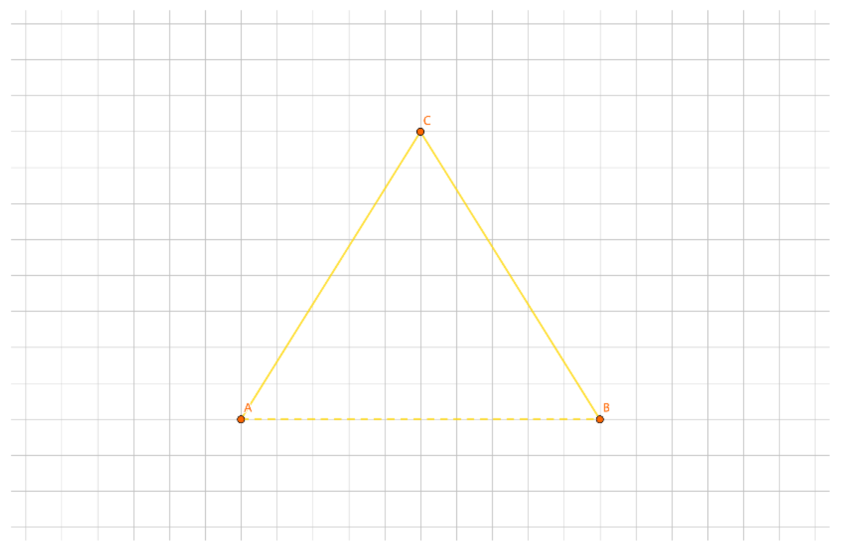
Figure 2.
Example of Convex Hull.
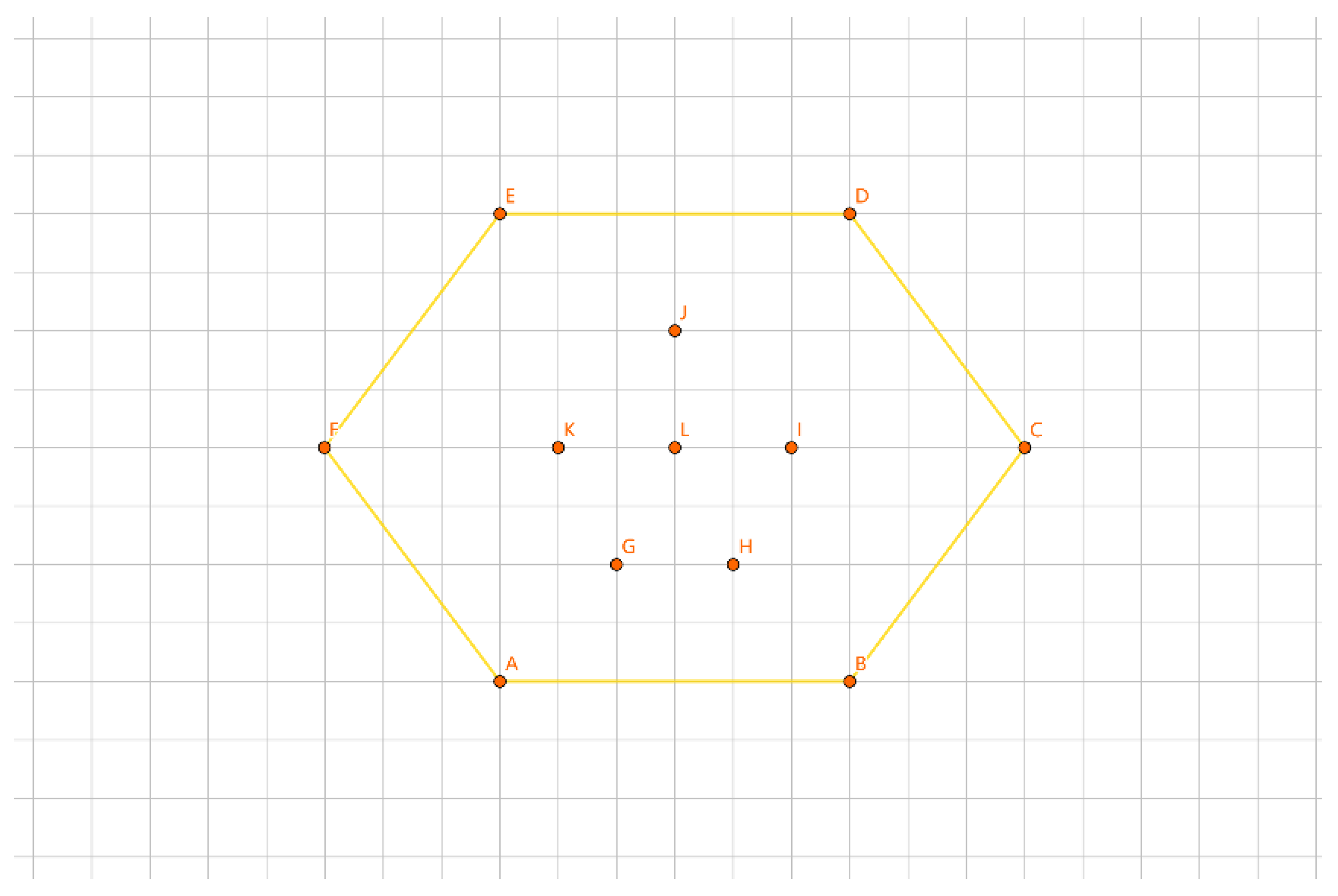
Figure 3.
Example of Convex Hull Layer.
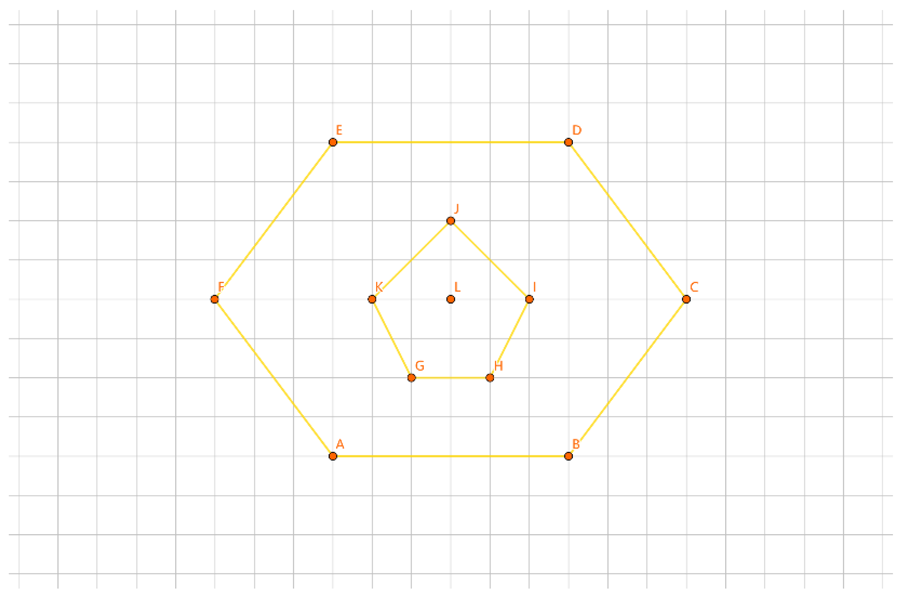
Figure 4.
Example of Single-Layer Convex Hull.
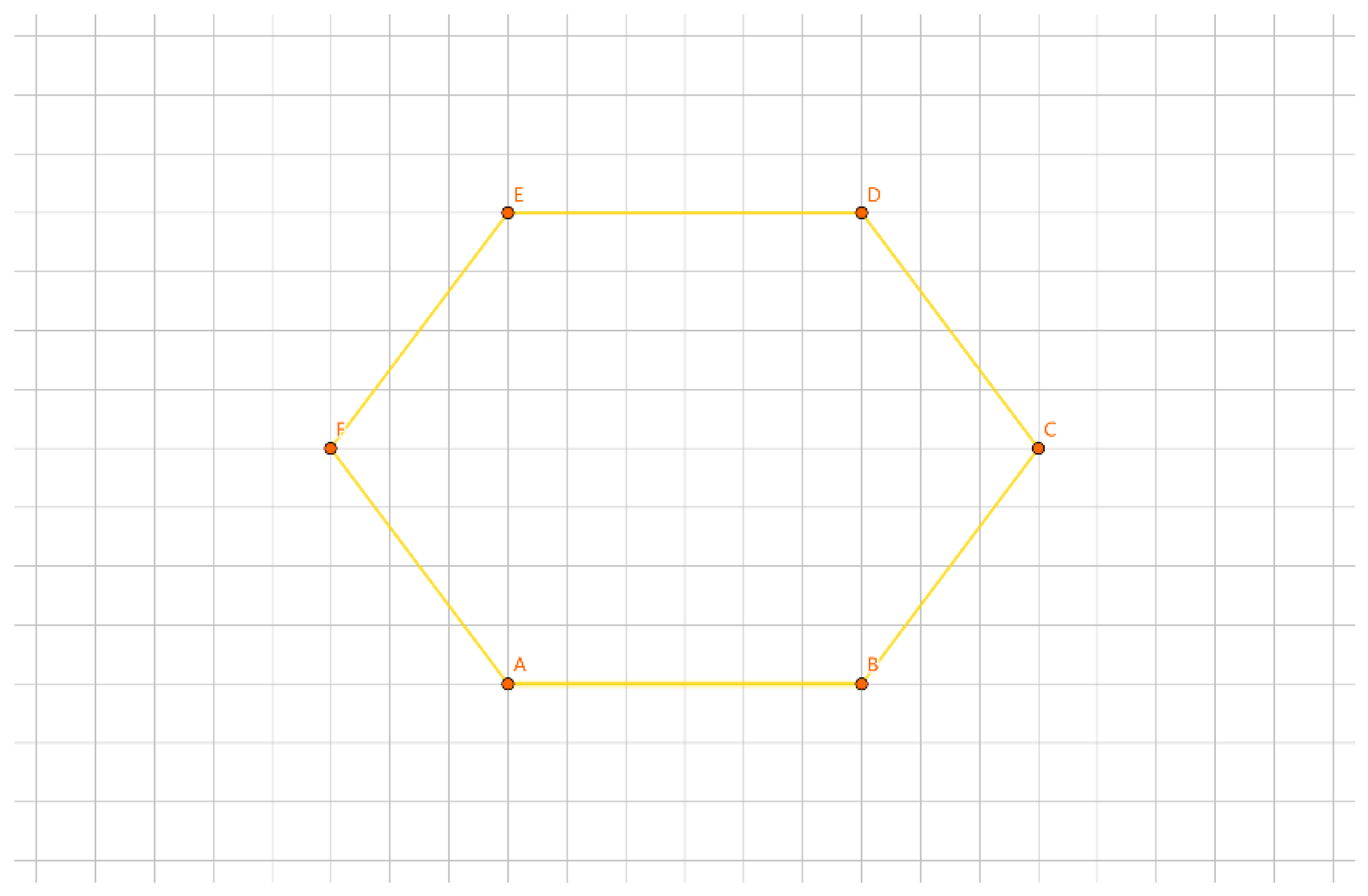
Figure 5.
Example of Two-Layer Convex Hull.
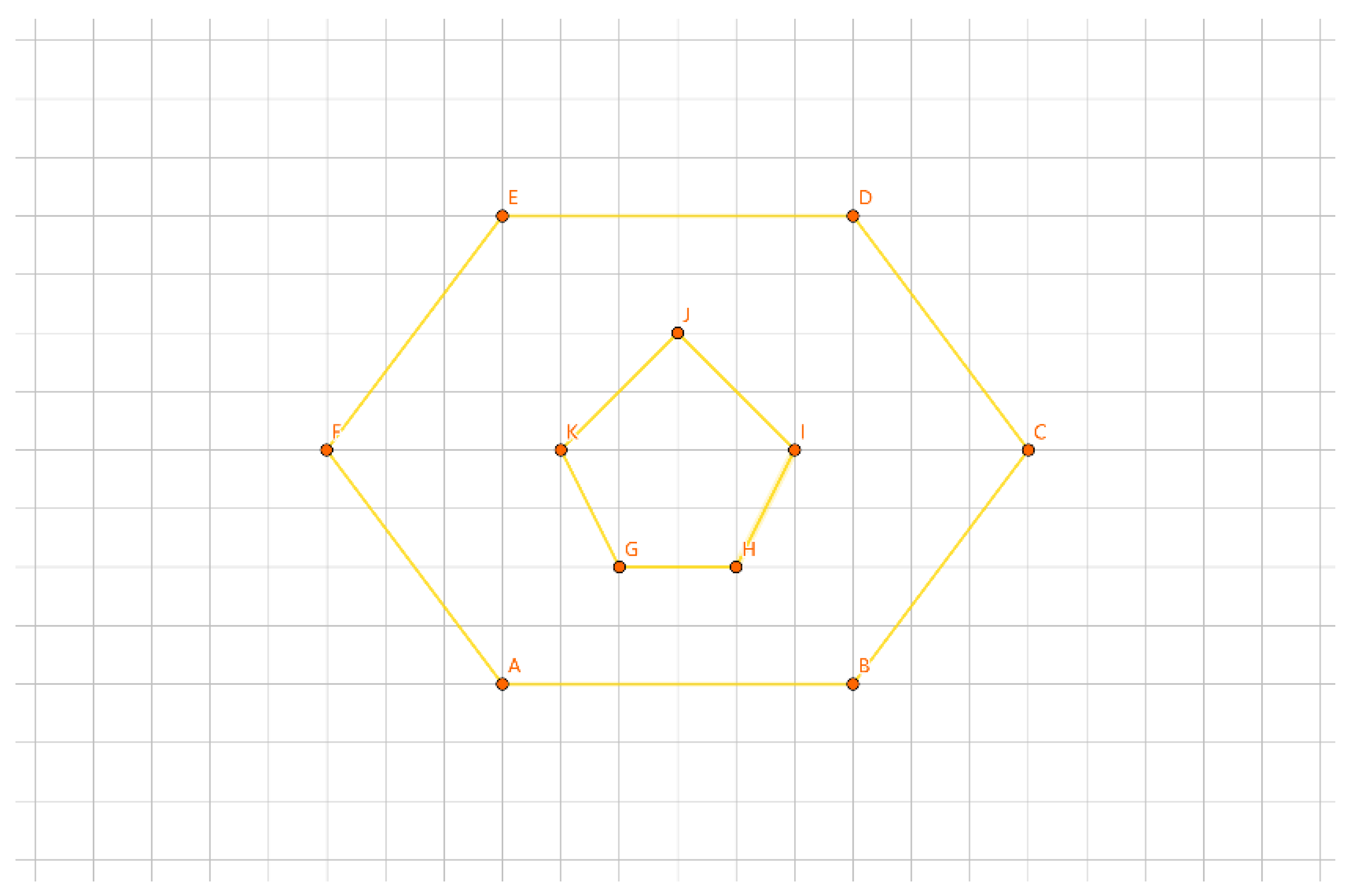
Figure 6.
Example of Multi-Layer Convex Hull.
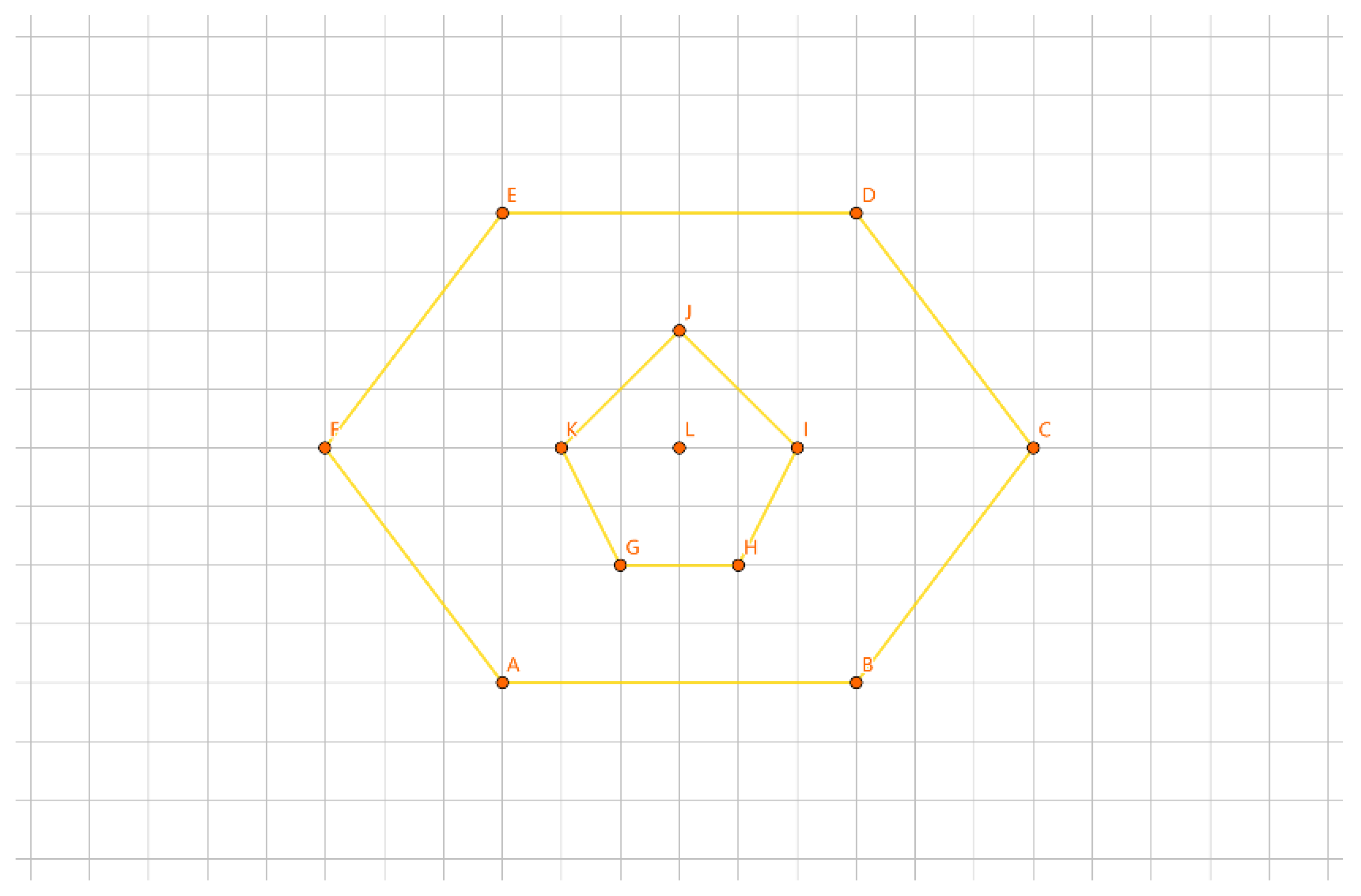
Figure 7.
Example of Inner and Outer Loops.
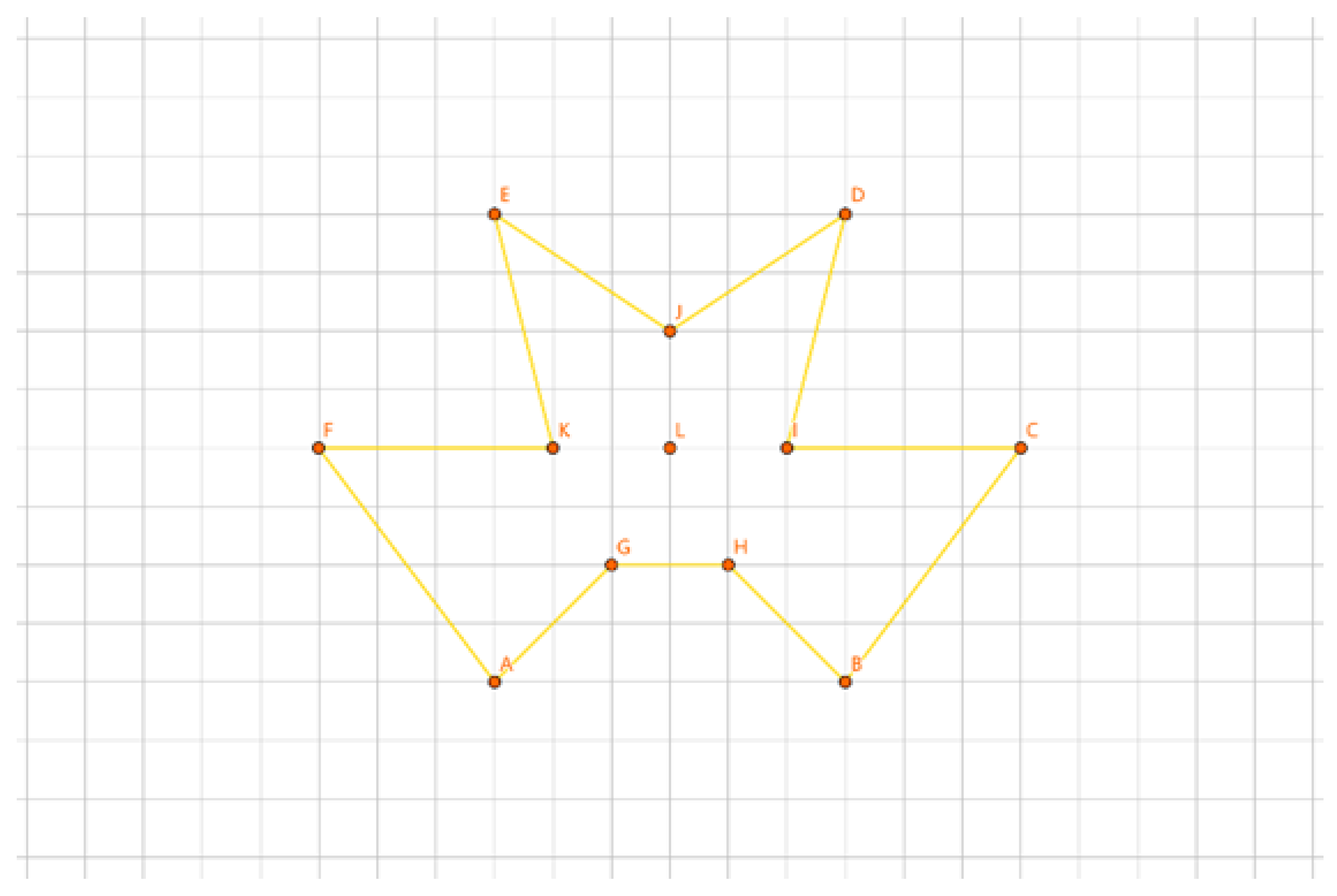
Figure 8.
Example of Groups.
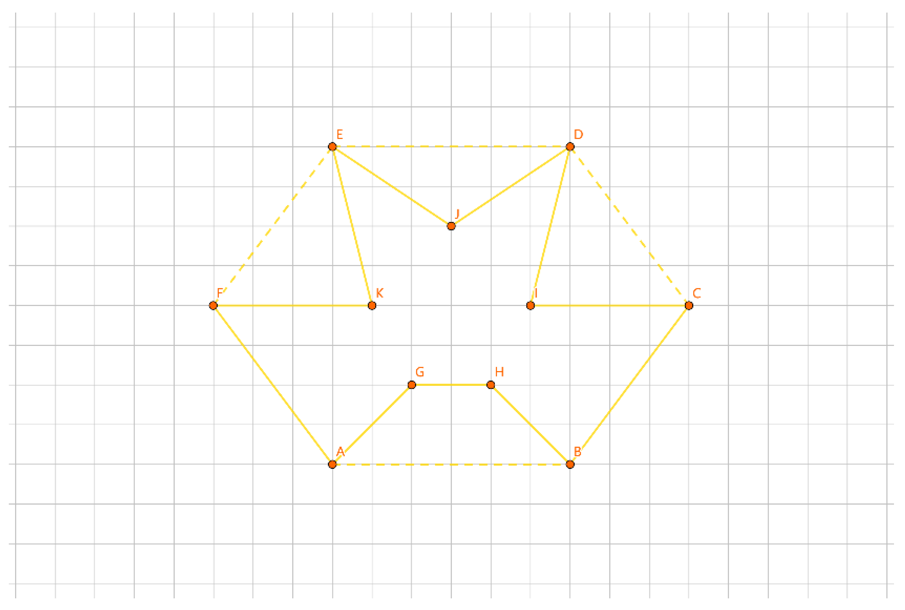
Figure 9.
Example illustrating Theorem 1.
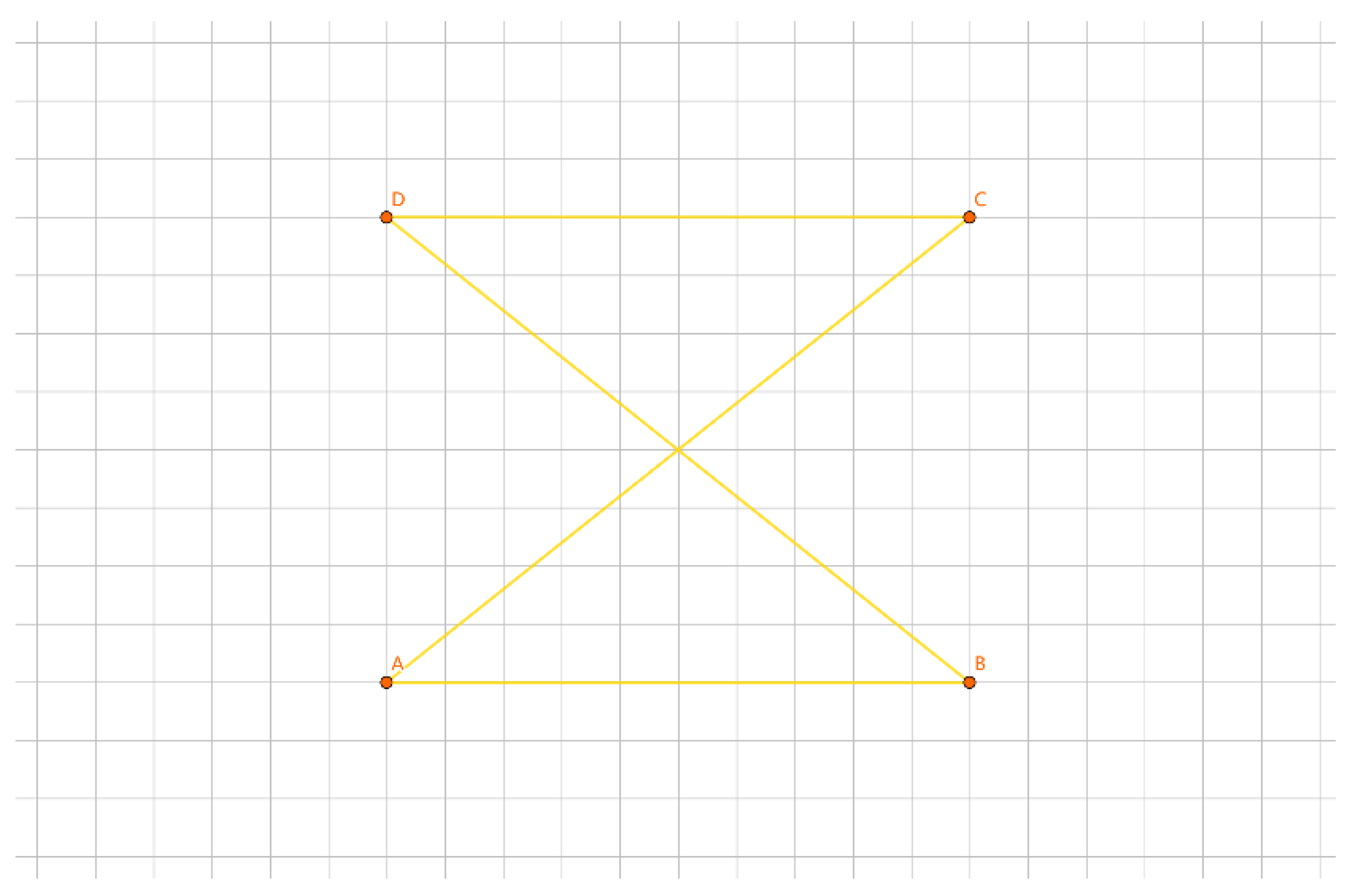
Figure 10.
Example illustrating Theorem 2.
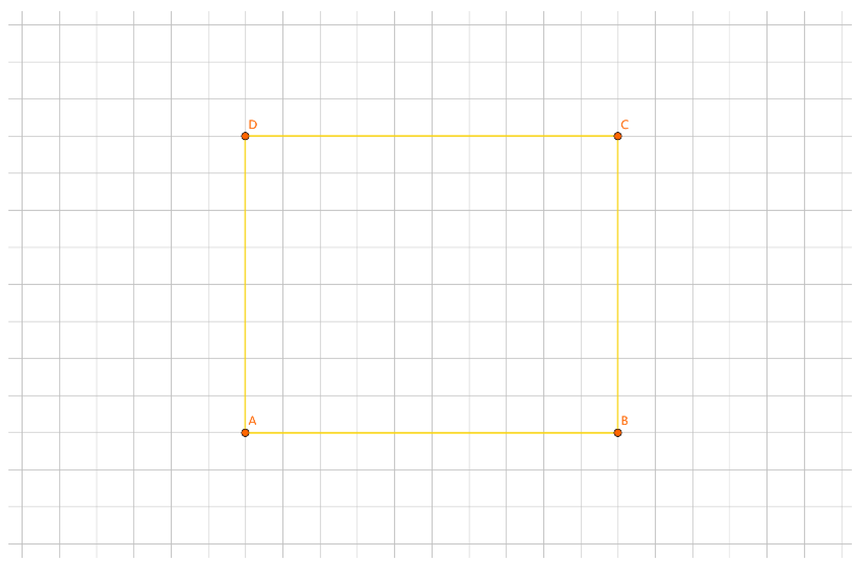
Figure 11.
Example illustrating Theorem 3.
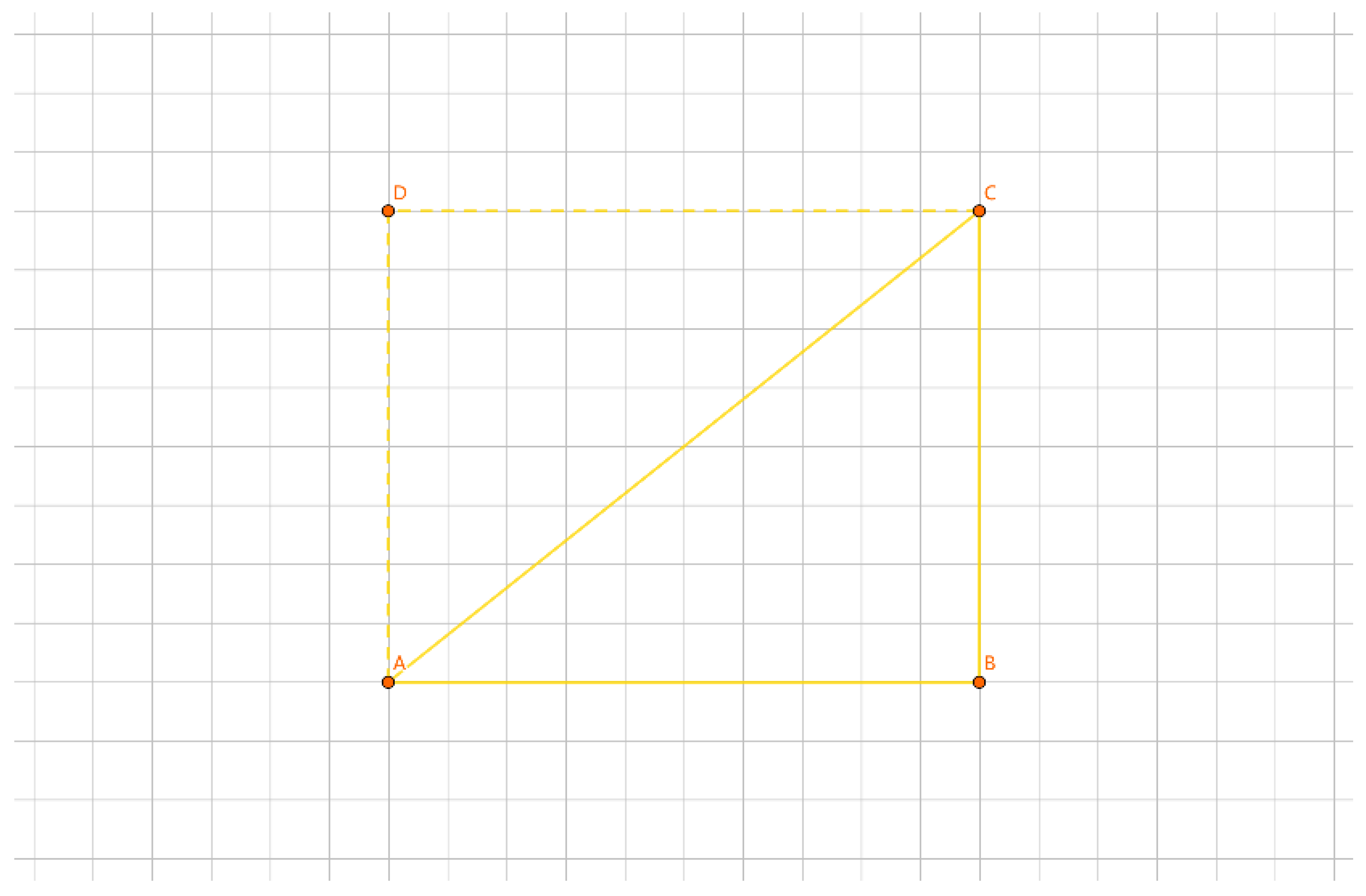
Figure 12.
illustrates Assumption 1.
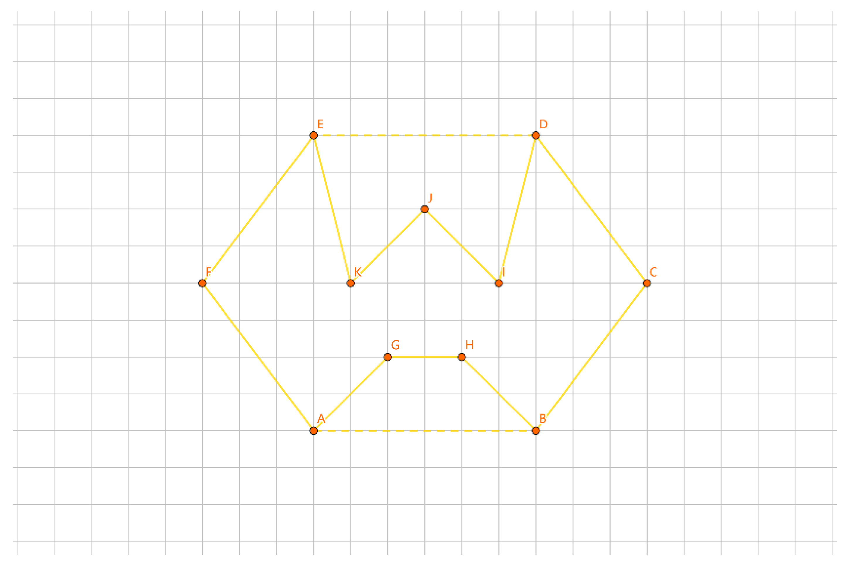
Figure 13.
illustrates a counterexample of Assumption 1.
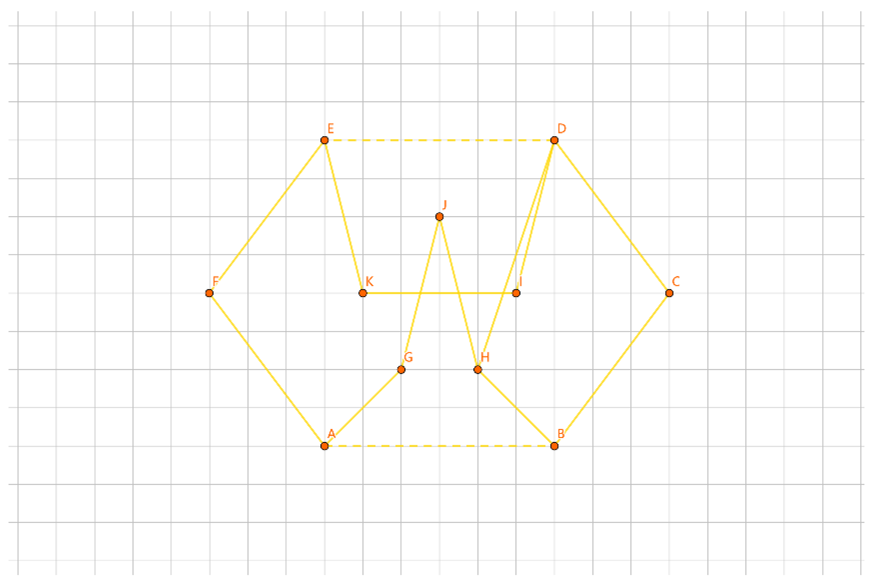
Figure 14.
illustrates Assumption 2.
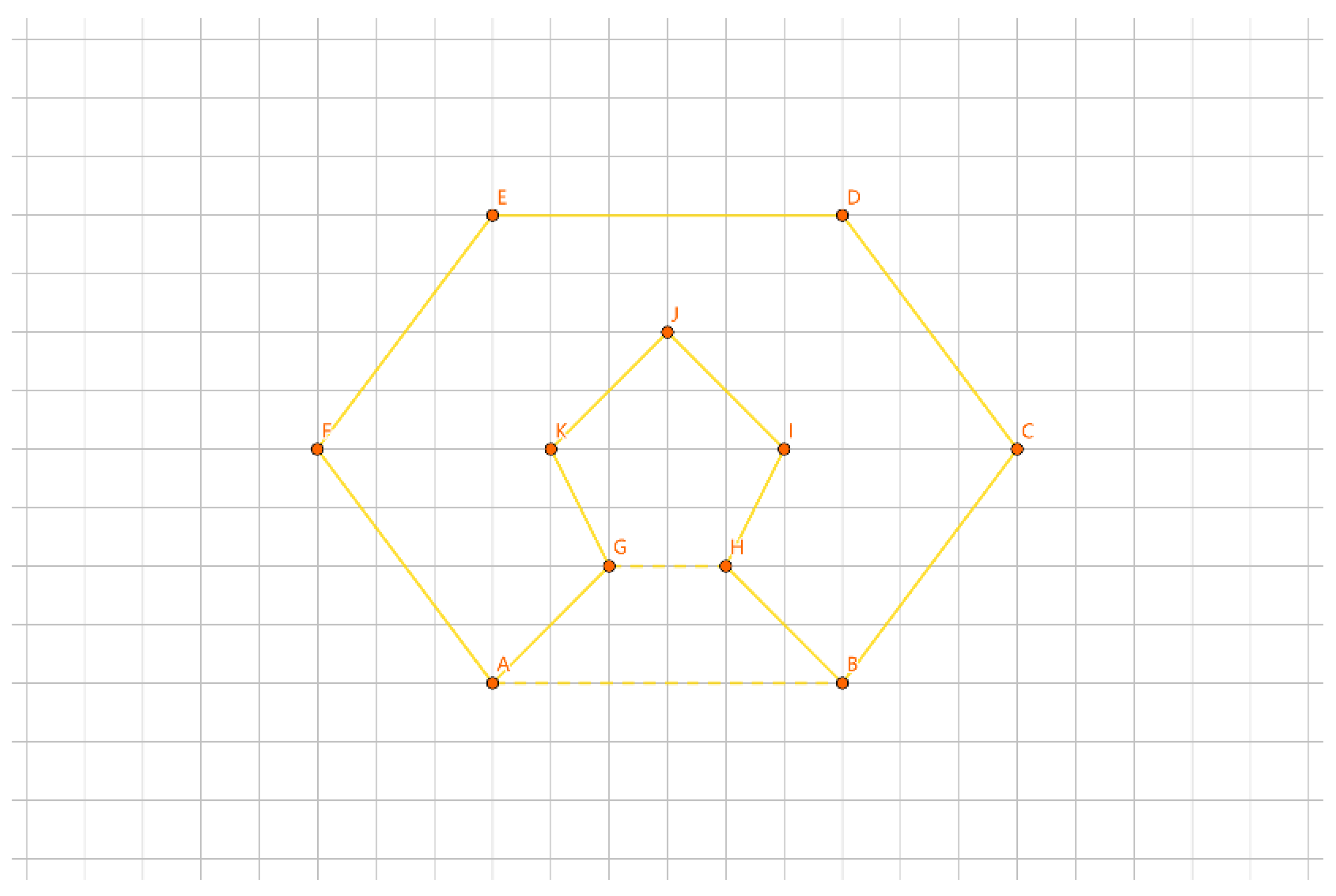
Figure 15.
illustrates Assumption 3.
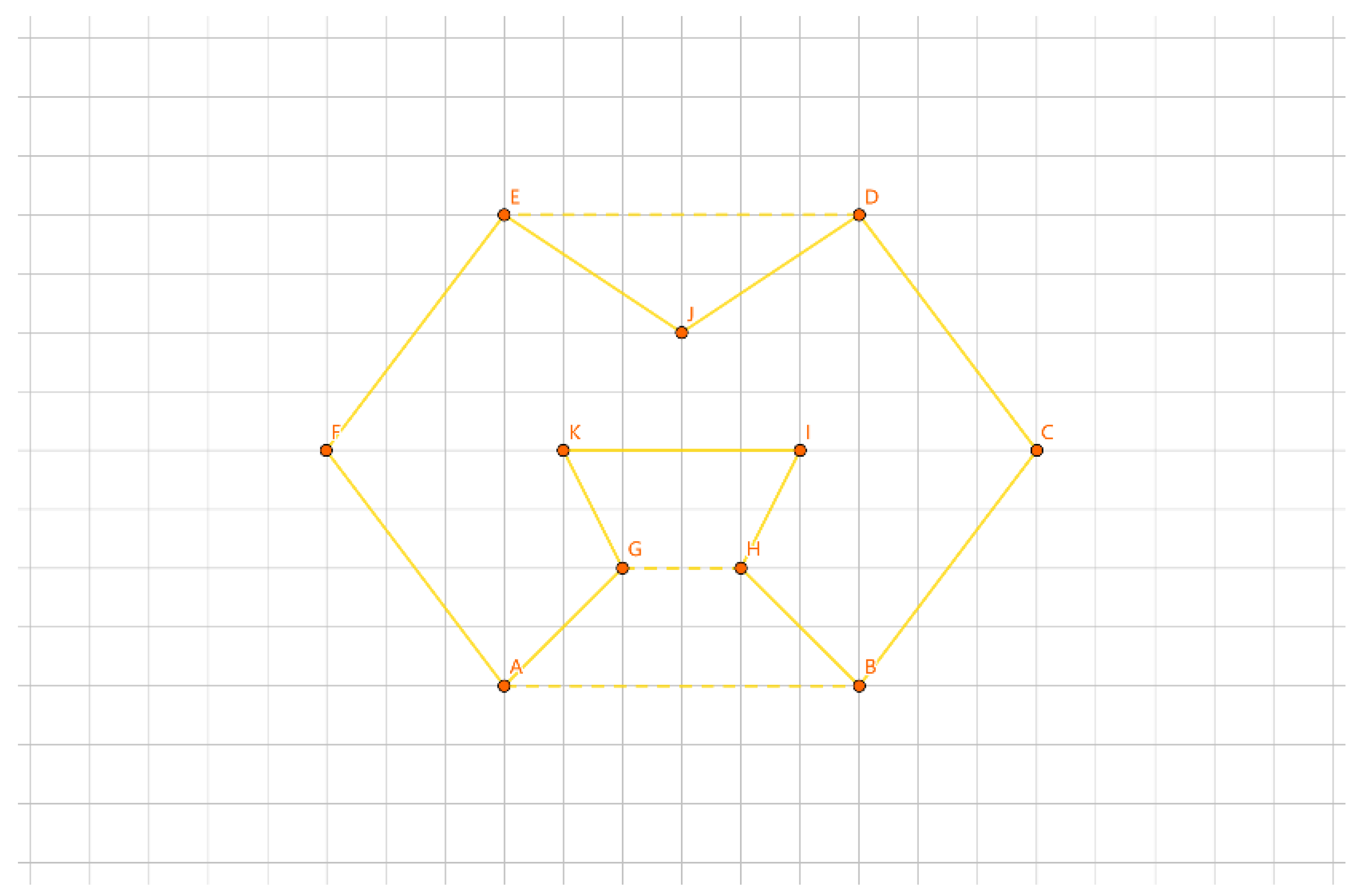
Figure 16.
Single Convex Hull Layer.
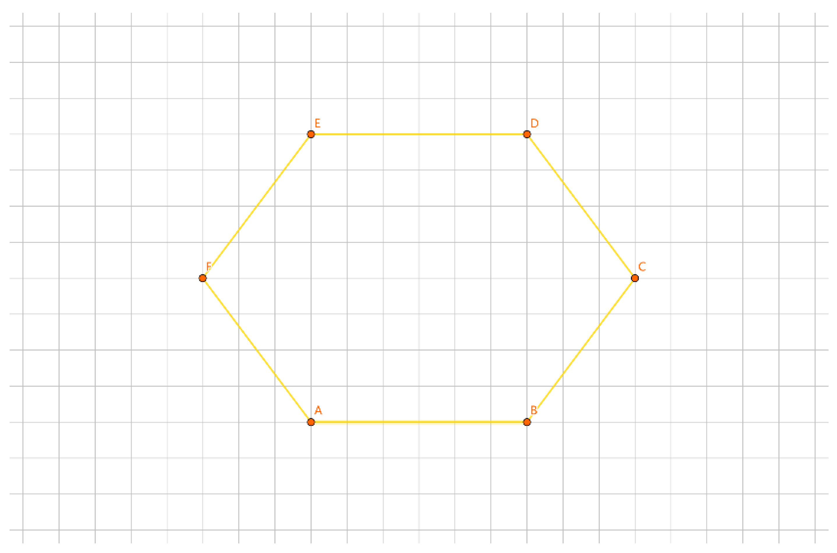
Figure 17.
Two Convex Hull Layers.
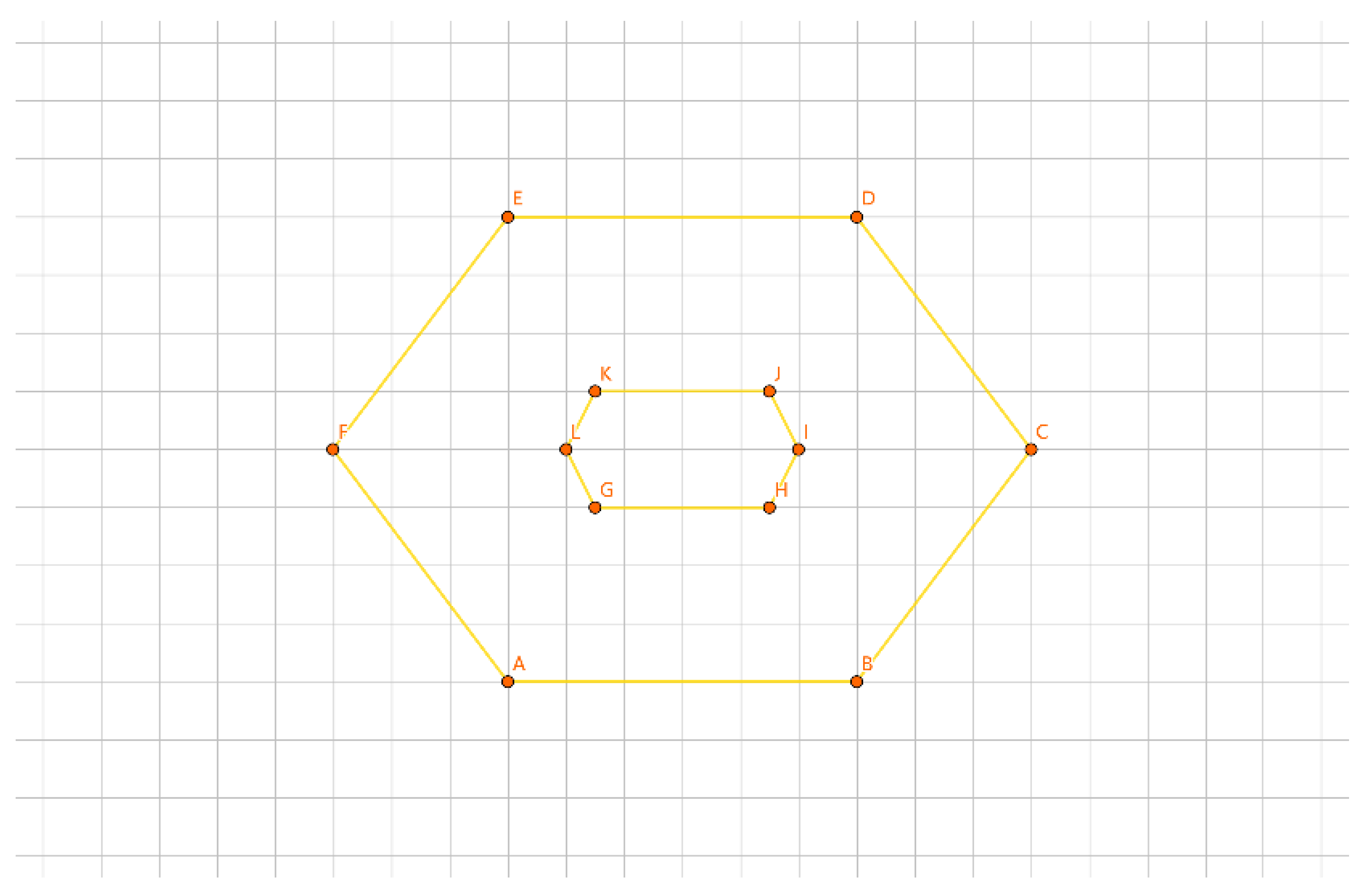
Figure 18.
Example Related to the Conclusion.
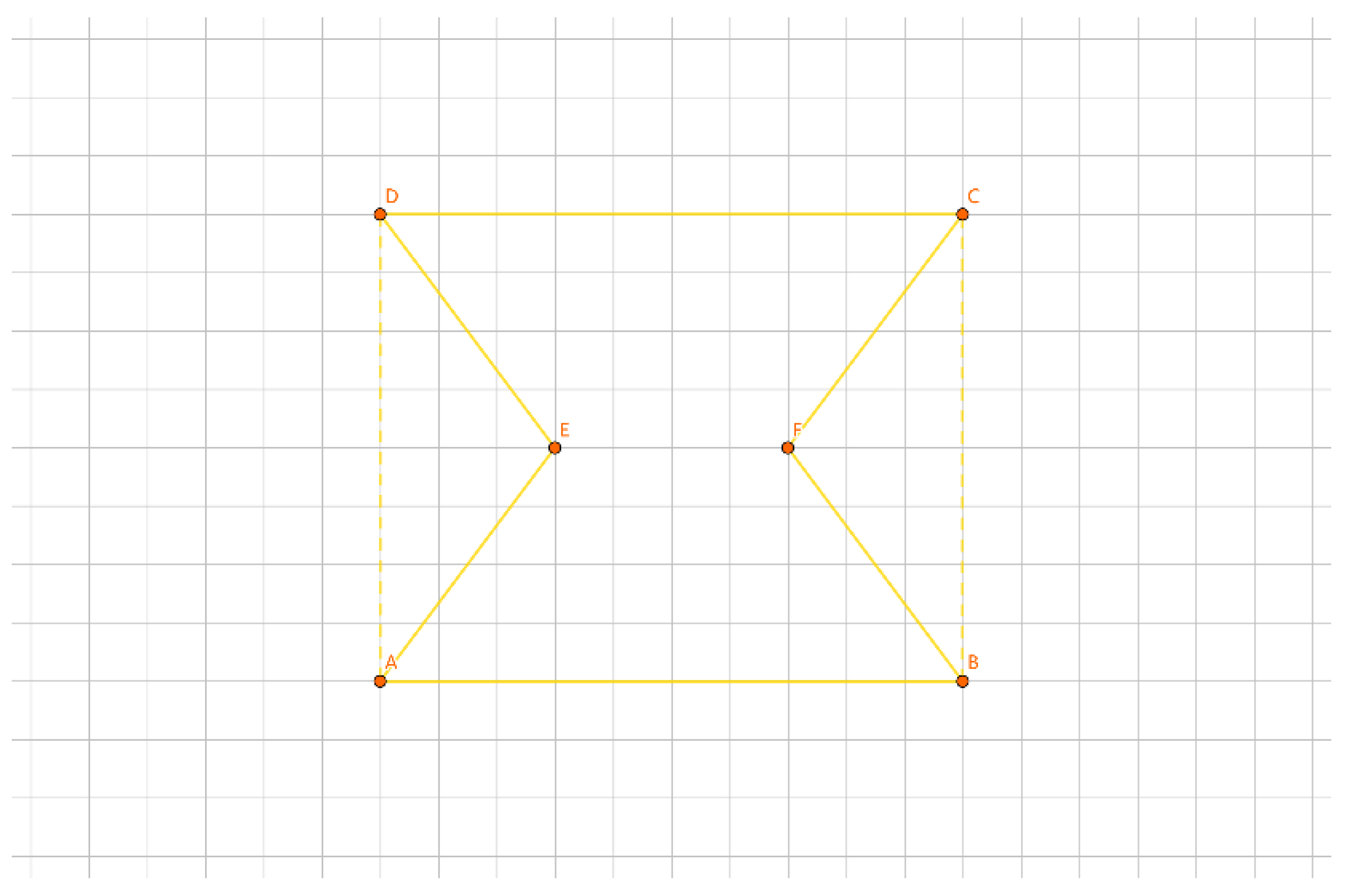
Figure 19.
Insertion Method for Groups.
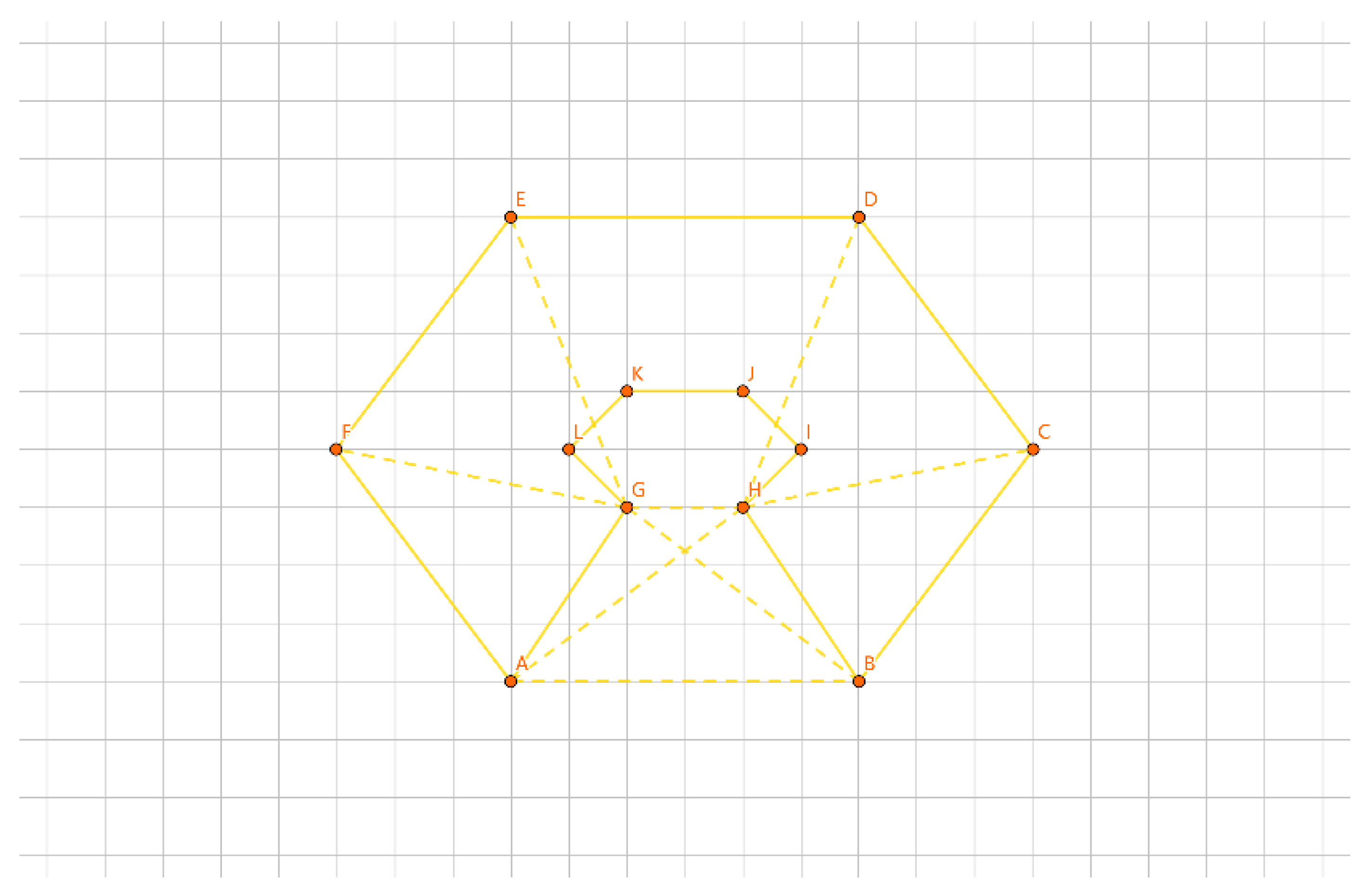
Figure 20.
Concise Representation.
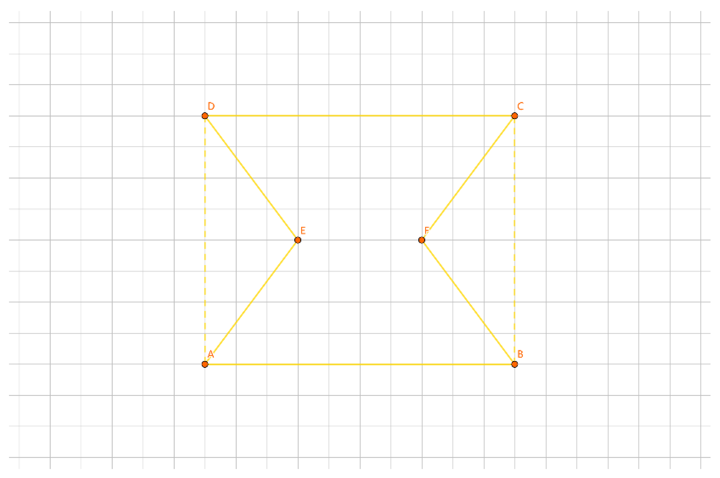
Figure 21.
Pairwise Grouping.
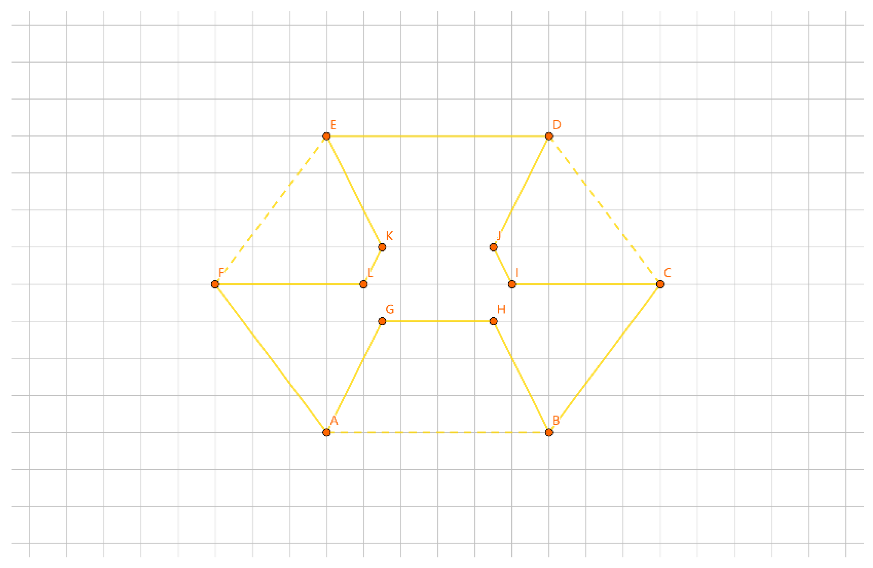
Figure 22.
First Test.
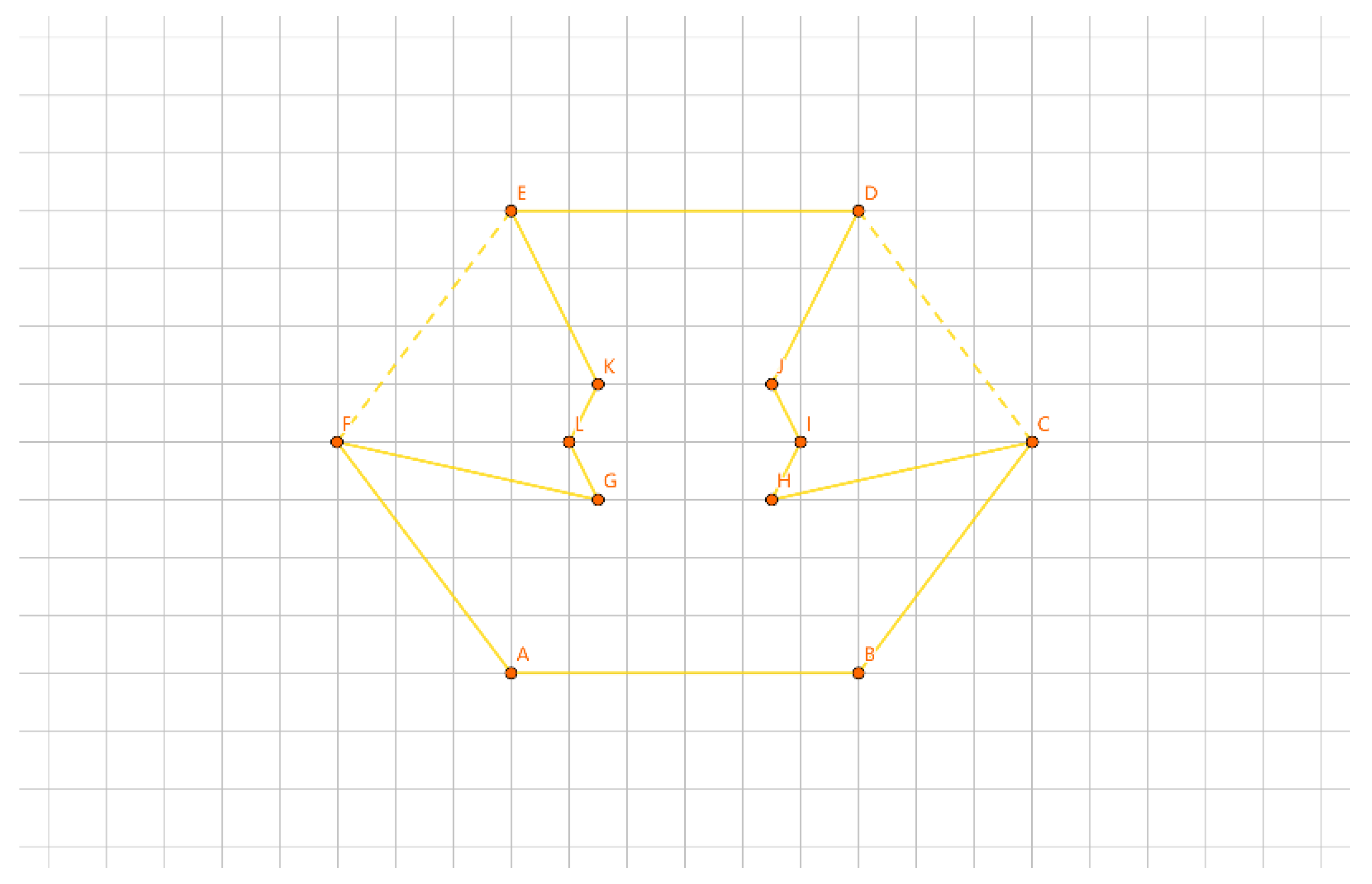
Figure 23.
Second Test.
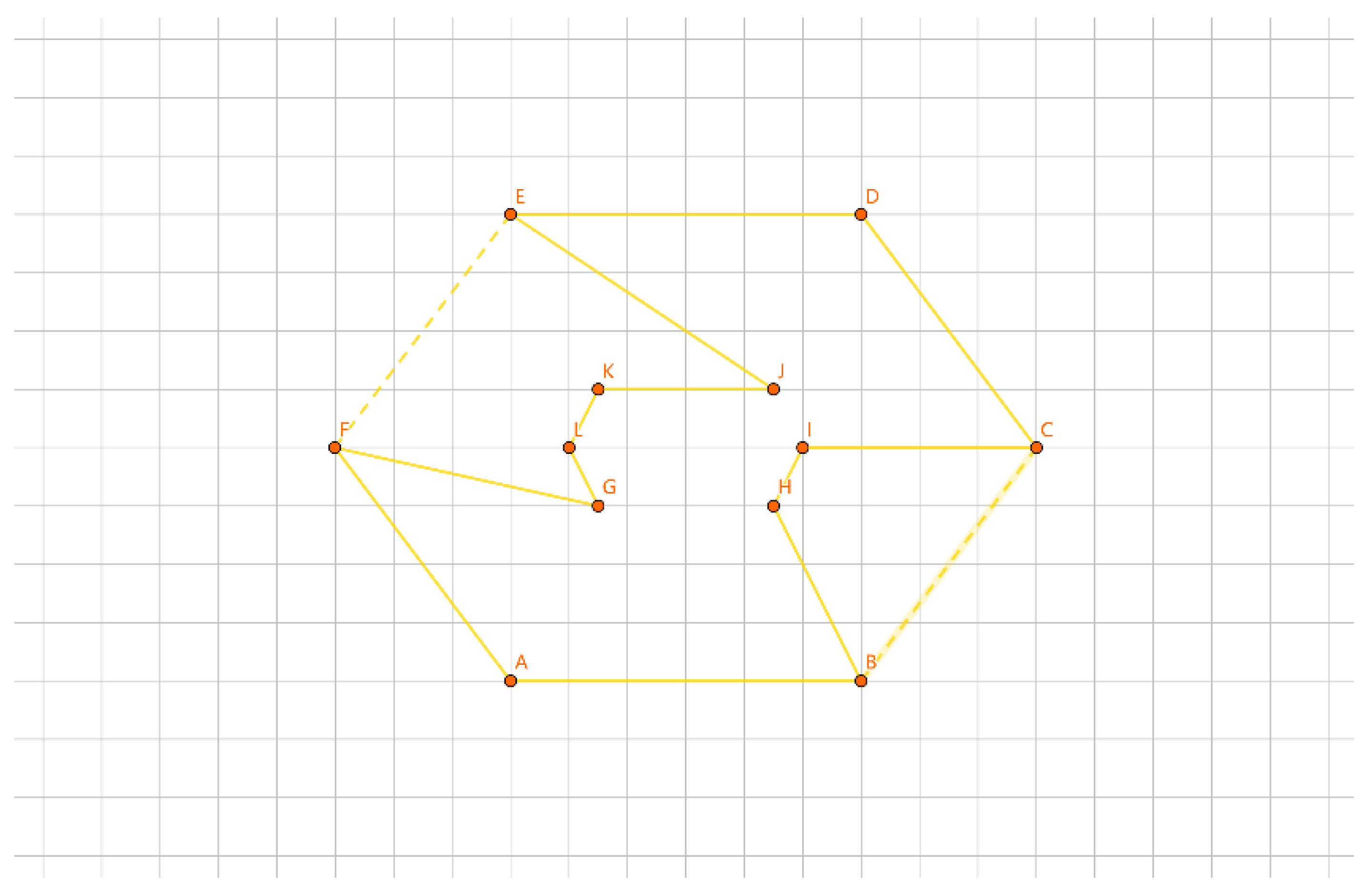
Figure 24.
Third Test.
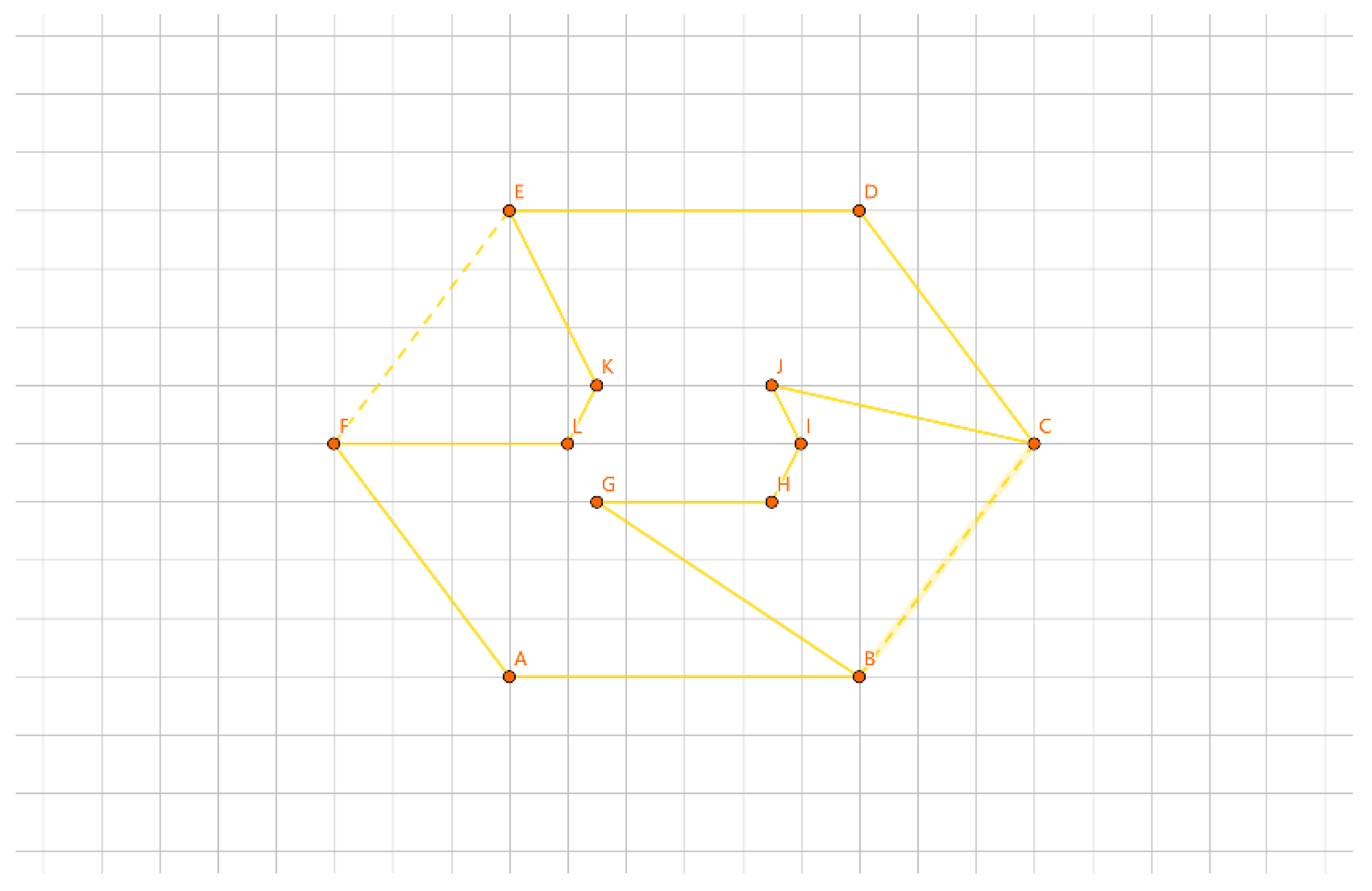
Figure 25.
Minimum Increment for Groups with Two or Three Points.
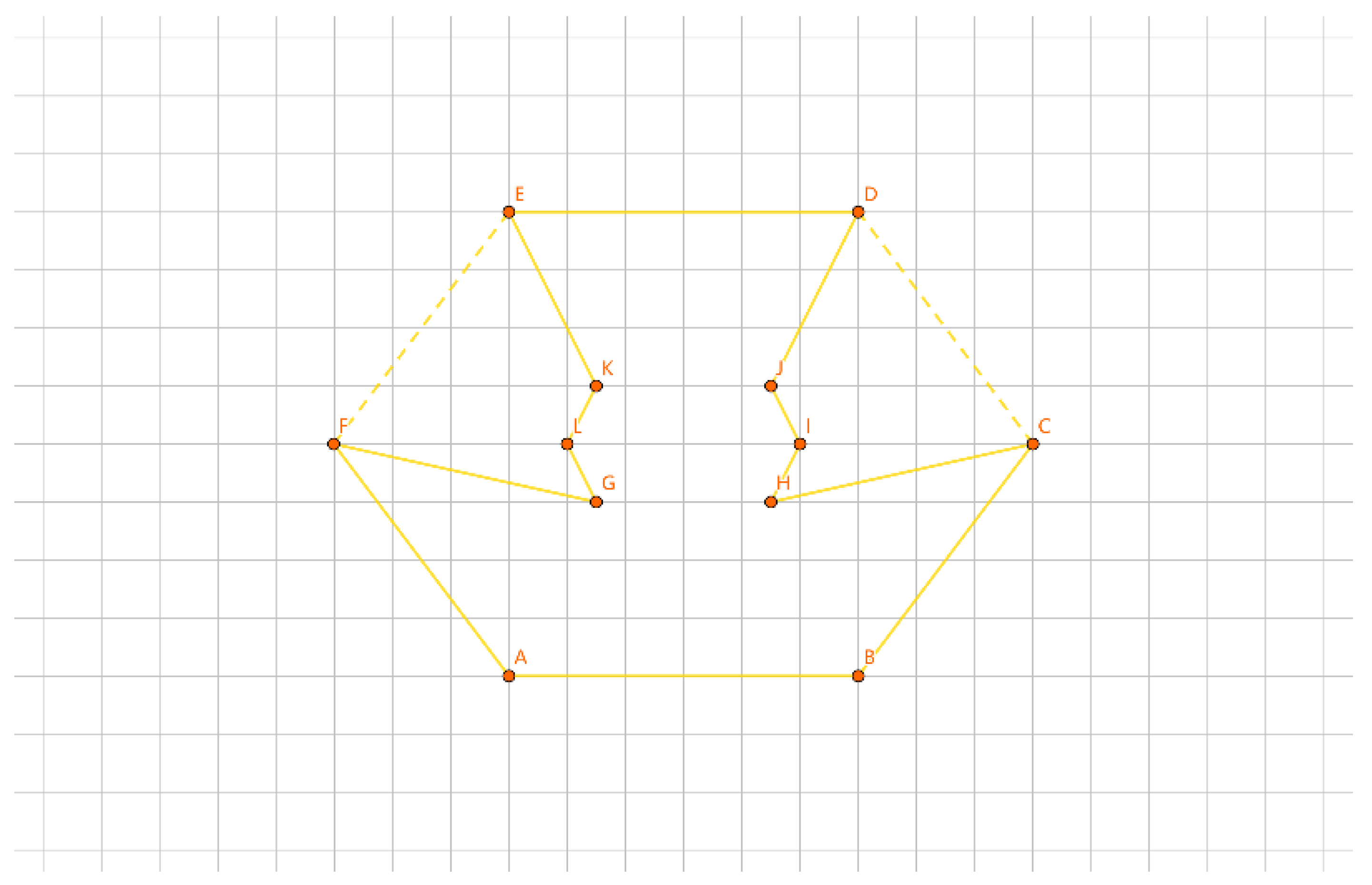
Figure 26.
Minimum Increment for Groups with More Than One Point.
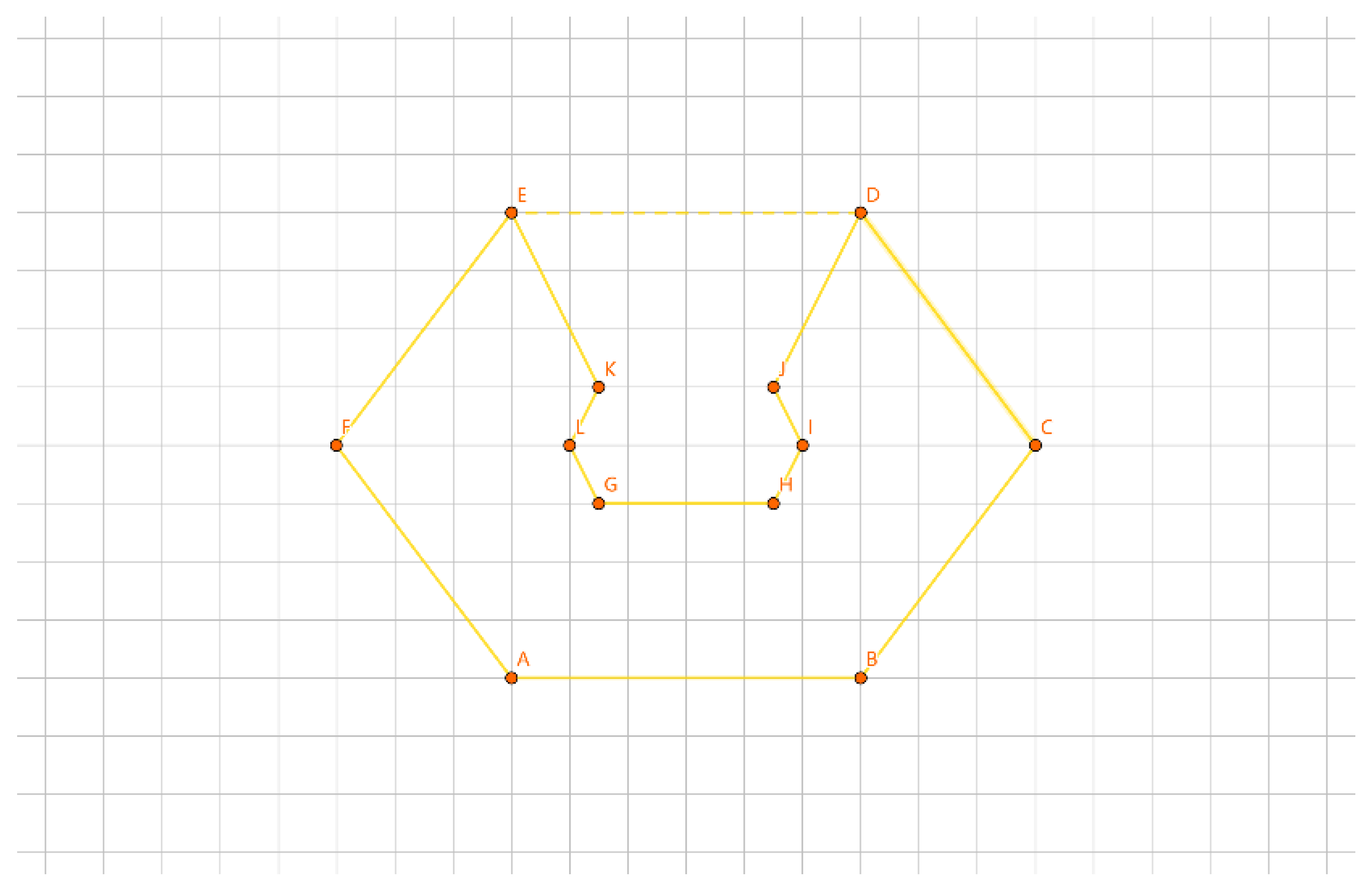
Figure 27.
Overall Minimum Increment.
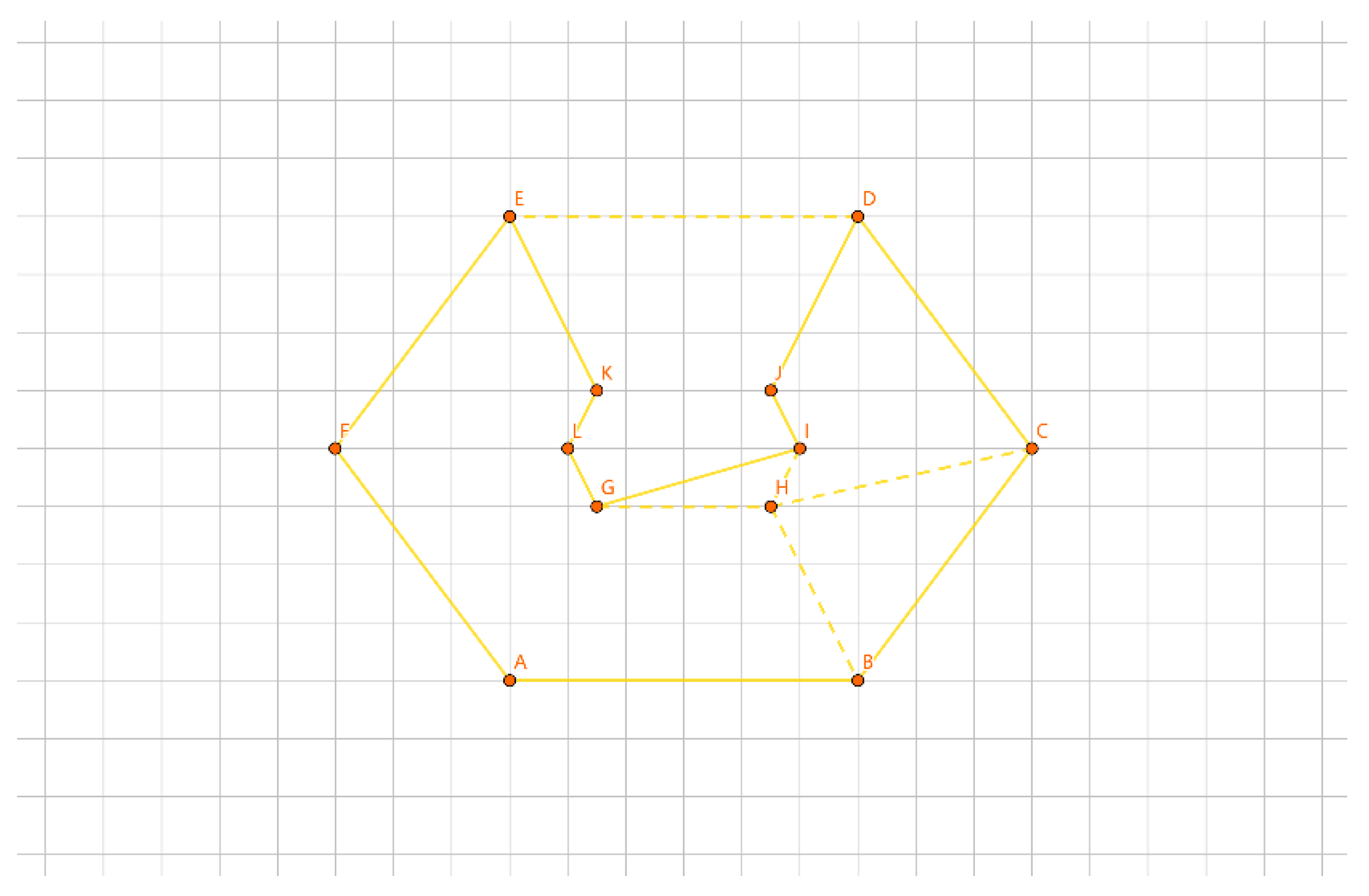
Figure 28.
Multiple Layers of Convex Hulls.
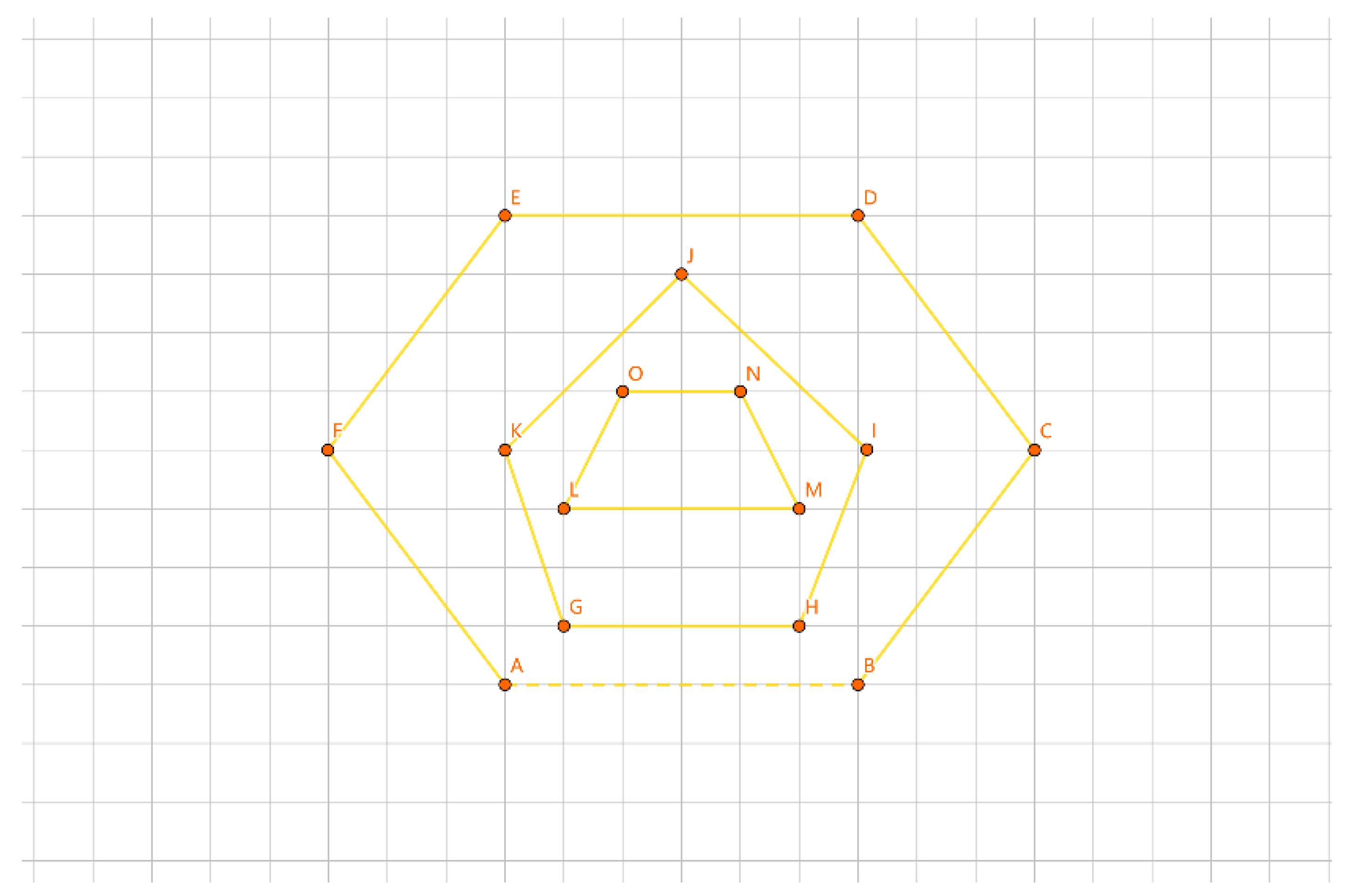
Figure 29.
First Merge.
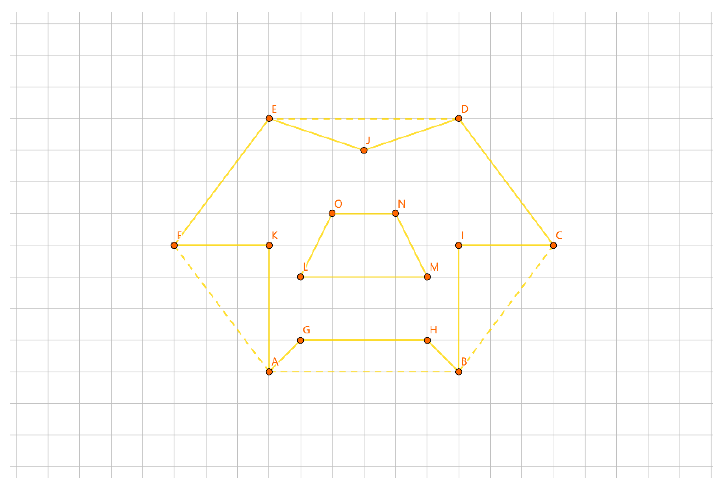
Figure 30.
Second Fusion.
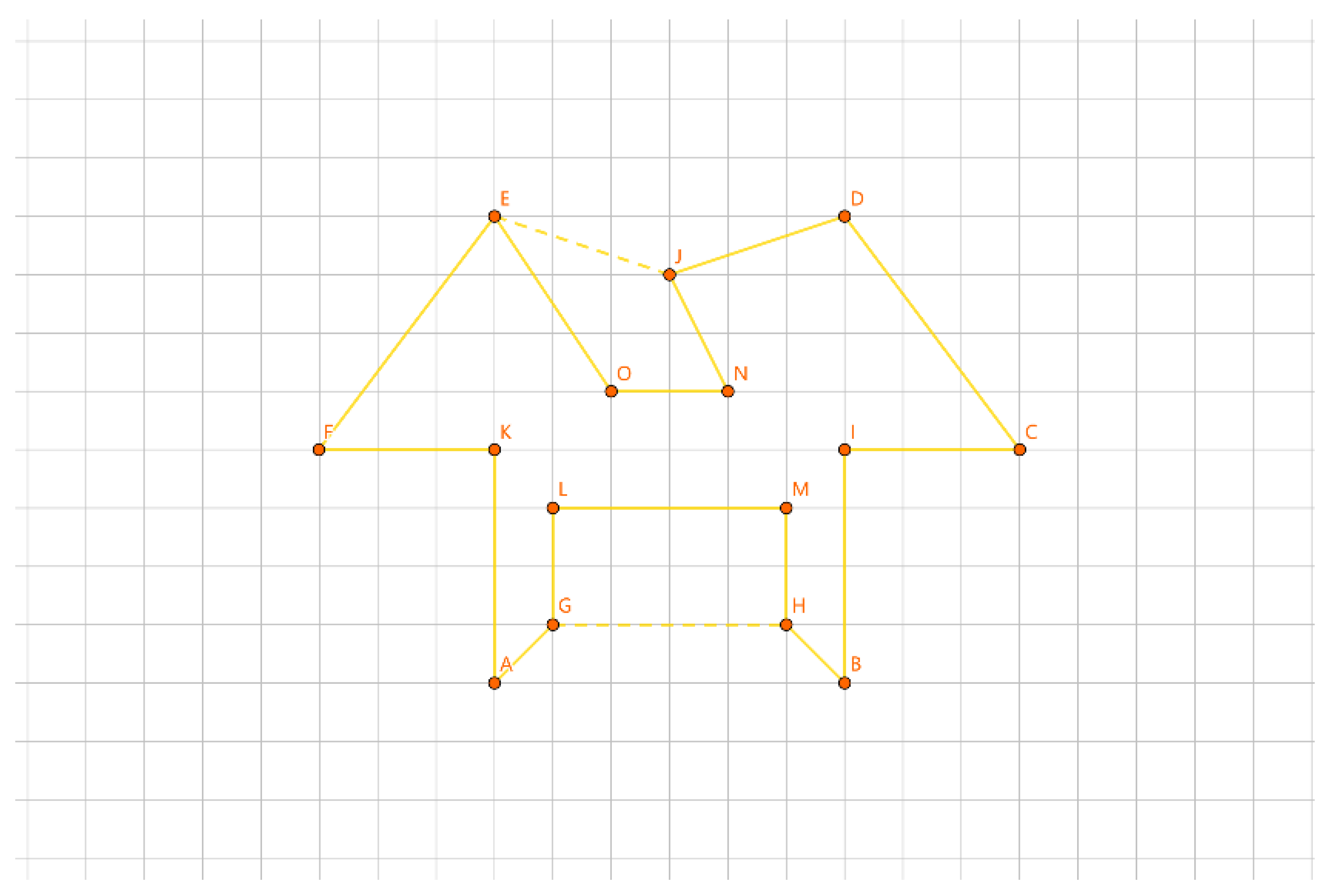
Figure 31.
Shorter Circuit.
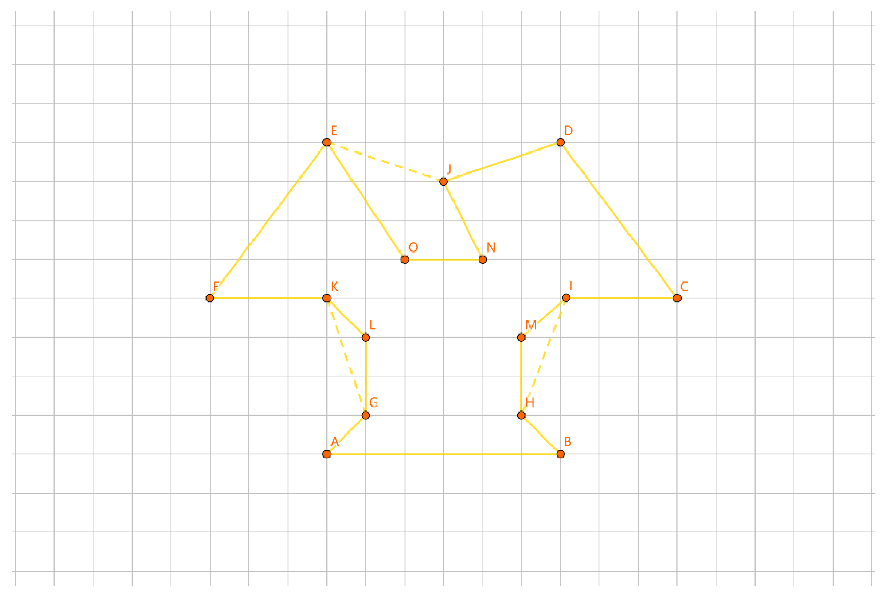
Figure 32.
Initial Circuit.
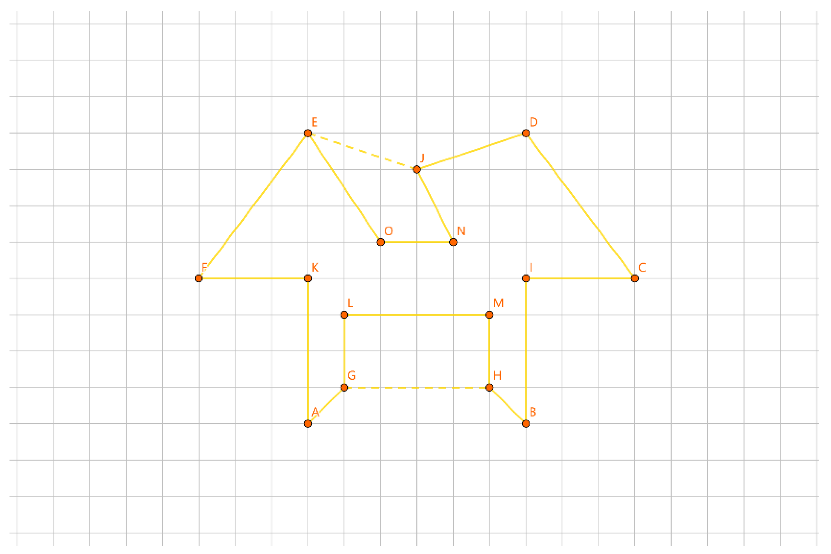
Figure 33.
Taking Segment G.
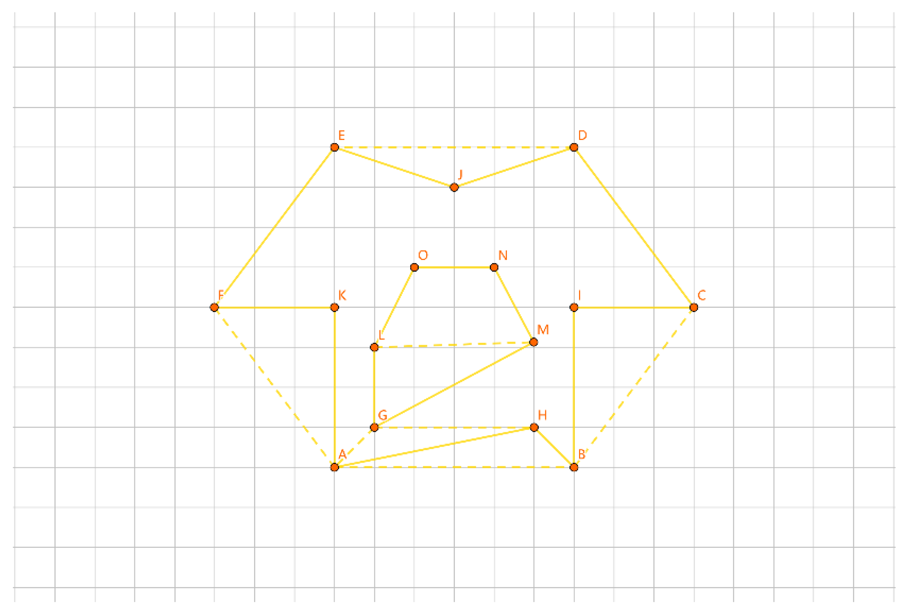
Figure 34.
Merging Segment G.
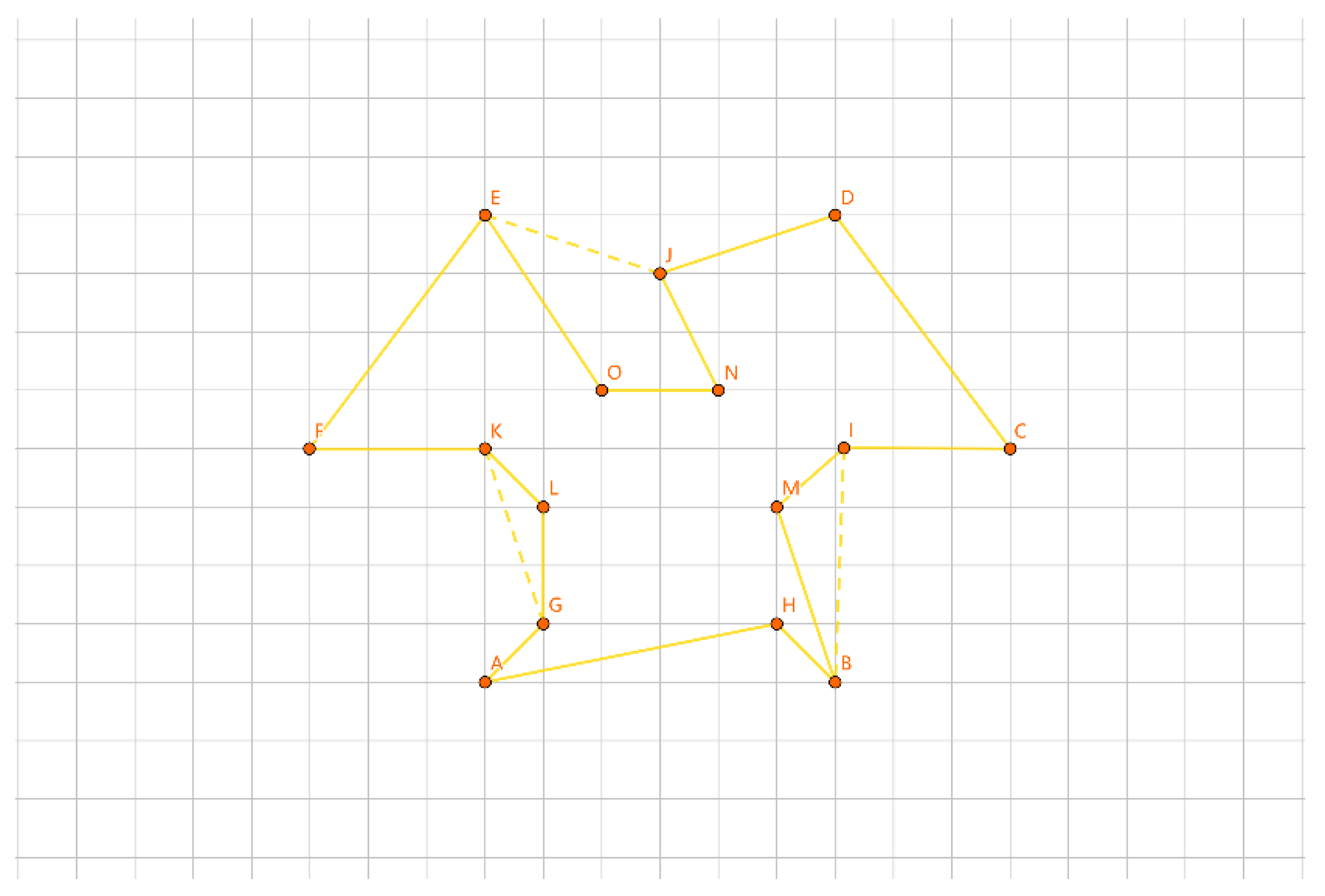
Figure 35.
Taking Segment GH.
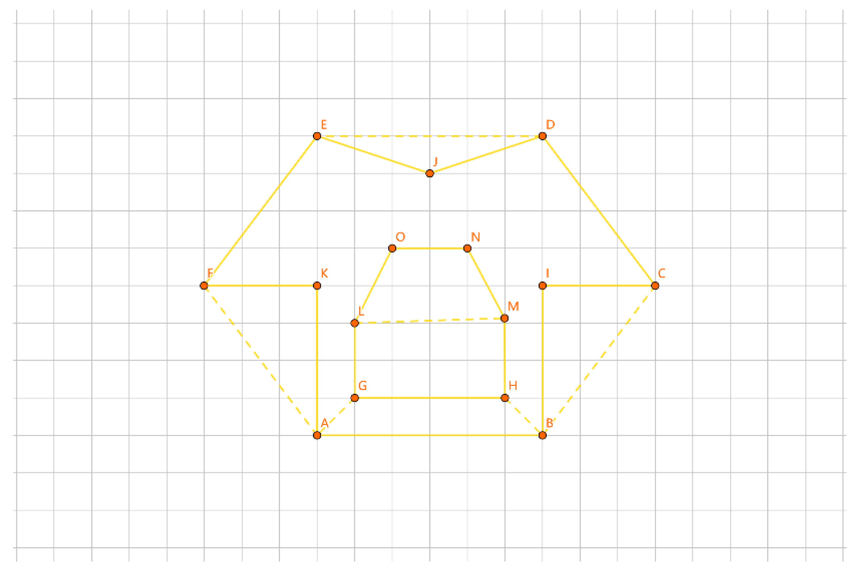
Figure 36.
Taking Segment GHB.
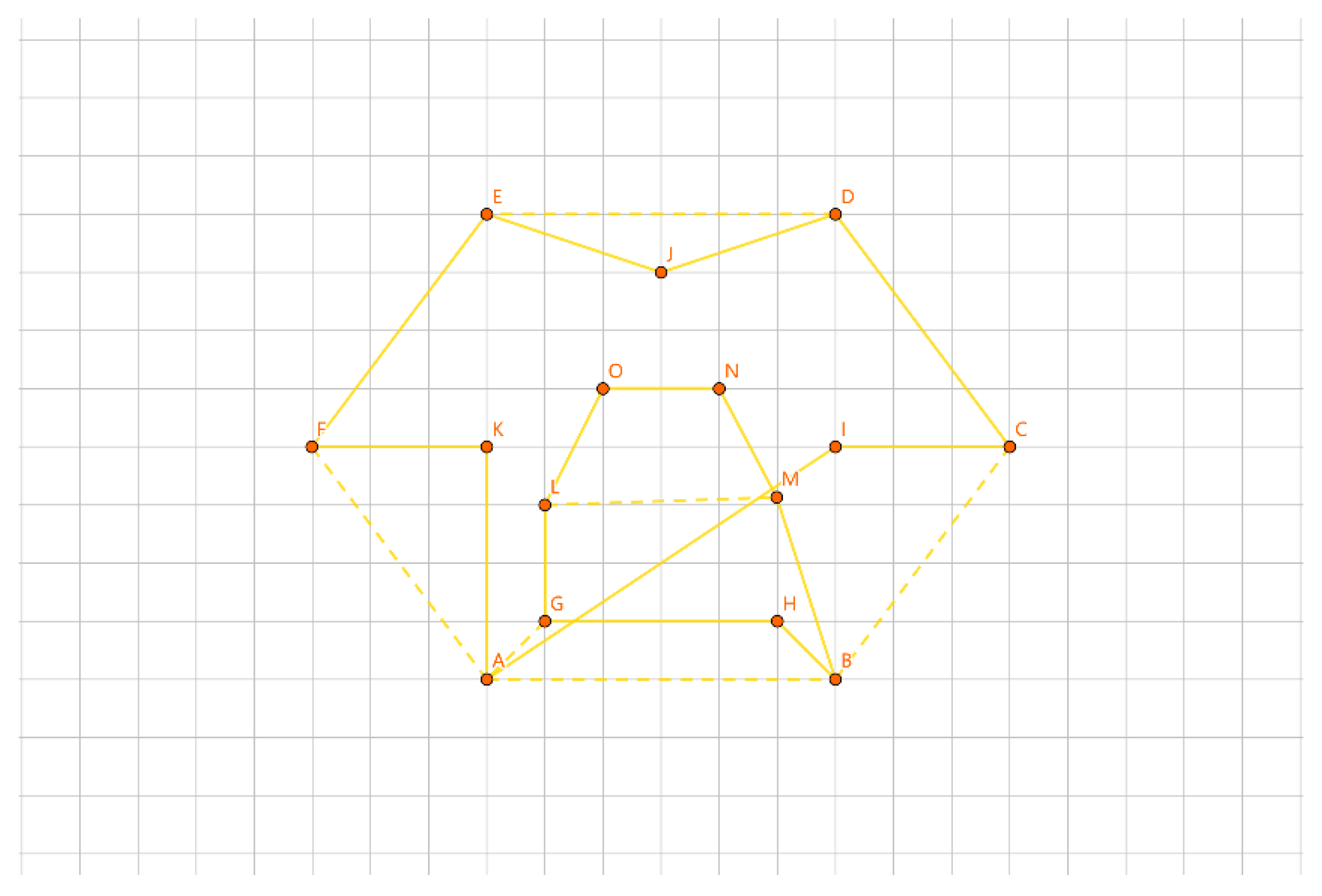
Figure 37.
Merged Result.

Figure 38.
Accuracy Evaluation Results.
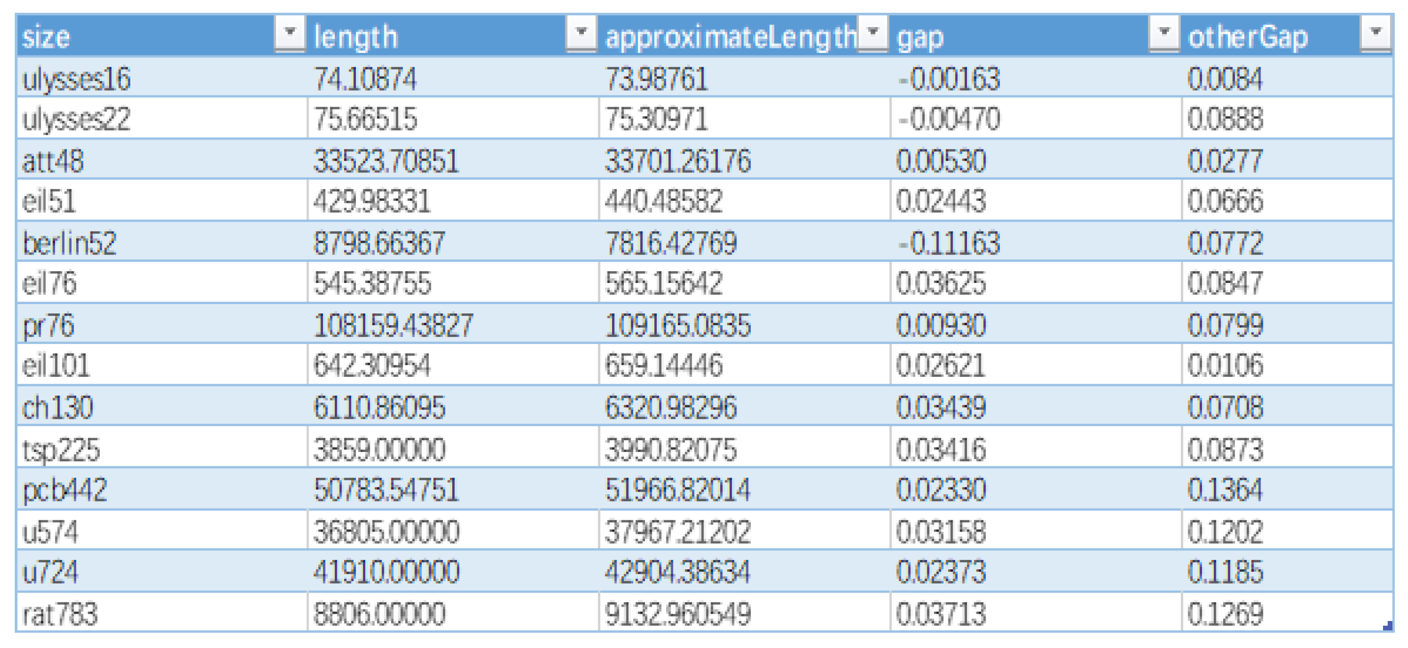
Figure 39.
Time Efficiency Evaluation Results.
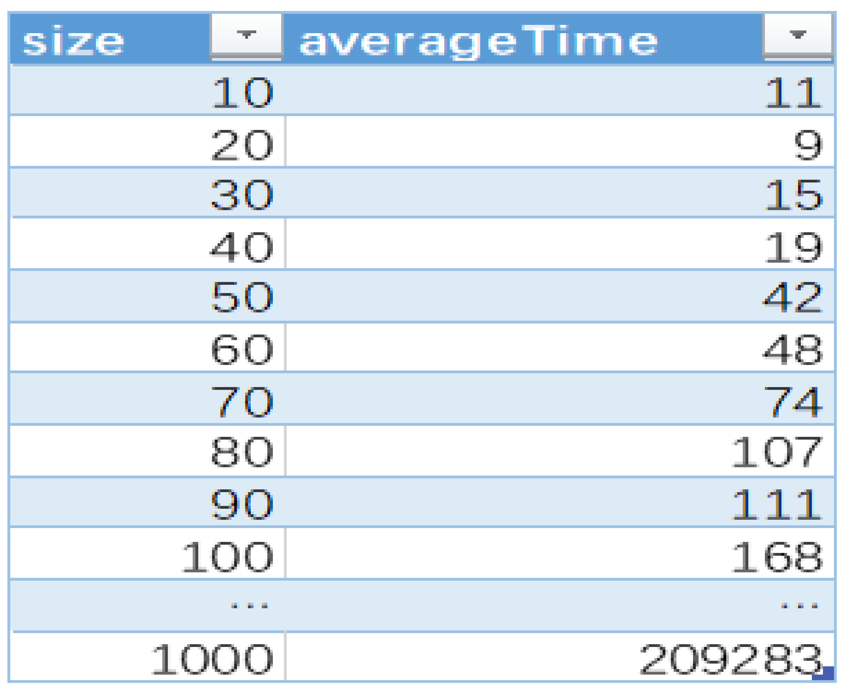
Figure 40.
Time Efficiency Evaluation Results.

Disclaimer/Publisher’s Note: The statements, opinions and data contained in all publications are solely those of the individual author(s) and contributor(s) and not of MDPI and/or the editor(s). MDPI and/or the editor(s) disclaim responsibility for any injury to people or property resulting from any ideas, methods, instructions or products referred to in the content. |
© 2024 by the author. Licensee MDPI, Basel, Switzerland. This article is an open access article distributed under the terms and conditions of the Creative Commons Attribution (CC BY) license (https://creativecommons.org/licenses/by/4.0/).
Copyright: This open access article is published under a Creative Commons CC BY 4.0 license, which permit the free download, distribution, and reuse, provided that the author and preprint are cited in any reuse.


