
Submitted:
30 May 2025
Posted:
04 June 2025
You are already at the latest version
Abstract
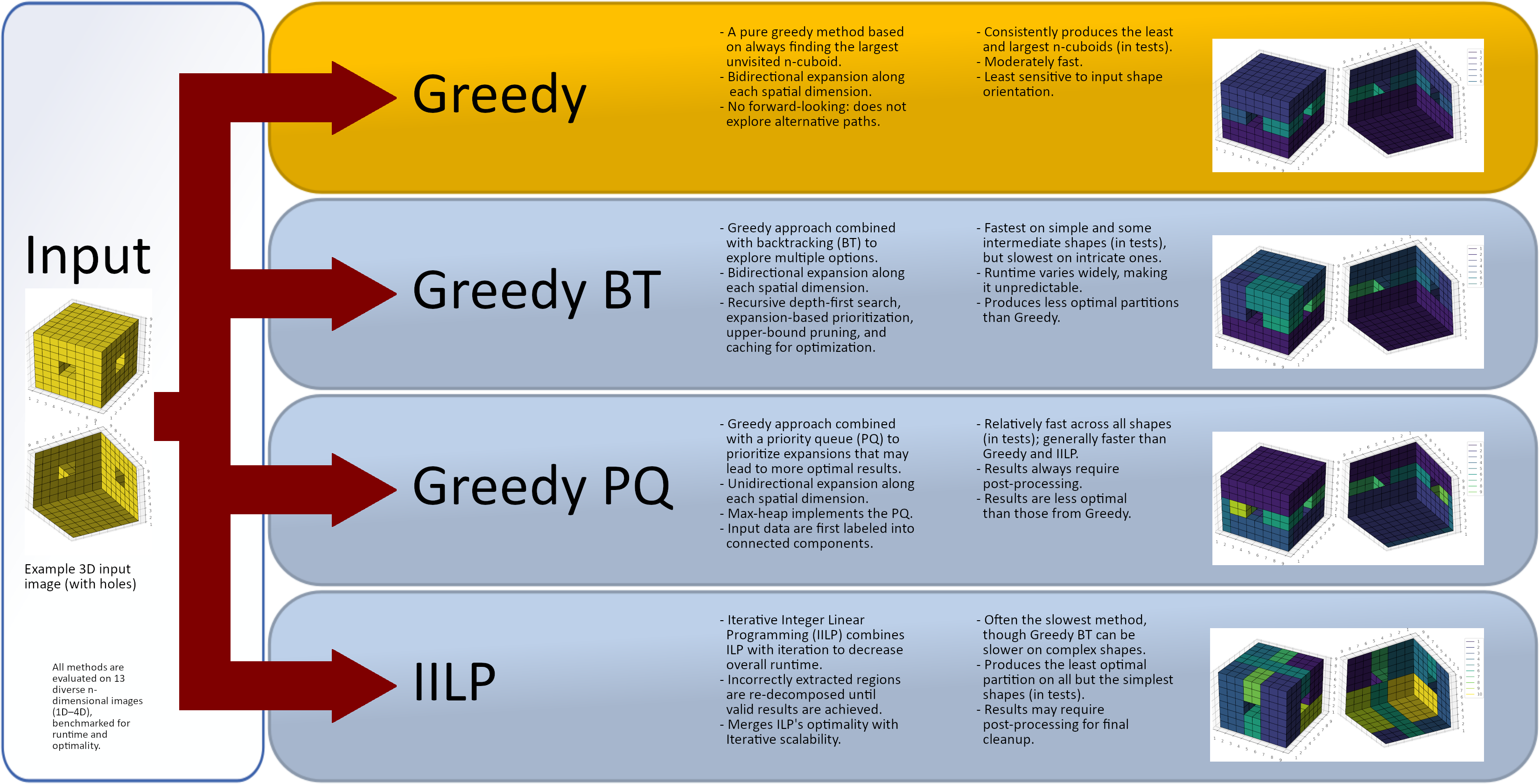
Partitioning rectangular and rectilinear shapes in n-dimensional binary images into the smallest set of axis-aligned n-cuboids is a fundamental problem in image analysis, pattern recognition, and computational geometry, with applications in object detection, shape simplification, and data compression. This paper introduces and evaluates four deterministic decomposition methods: pure greedy selection, greedy with backtracking, greedy with a priority queue, and an iterative integer linear programming (IILP) approach. These methods are benchmarked against three established baseline techniques across 13 diverse 1D–4D images (up to 8×8×8×8 elements) featuring holes, concavities, and varying orientations. Surprisingly, the simplest approach – a purely greedy heuristic selecting the largest unvisited region at each step – consistently achieved optimal or near-optimal decompositions, even for complex images, and maintained optimality under rotation without post-processing. By contrast, the more sophisticated methods (backtracking, prioritization, IILP) exhibited trade-offs between speed and quality, with IILP adding overhead without superior results. Runtime testing showed IILP was on average ~37× slower than the fastest greedy method (ranging from ~3× to 100× slower). These findings highlight that a well-designed greedy strategy can outperform more complex algorithms for practical binary shape decomposition, offering a compelling balance between computational efficiency and solution quality in pattern recognition and image analysis.
Keywords:
bitmap segmentation
; computational geometry
; greedy algorithms
; high-dimensional data
; image processing
; integer linear programming
; pattern recognition
; rectangular decomposition
1. Introduction
The polygon partition problem has been extensively studied, focusing on dividing rectangular and rectilinear shapes in n-dimensional bitmaps into simple, non-overlapping n-cuboids [1,2,3,4,5,6,7,8,9,10,11,12,13,14,15,16,17,18,19,20,21,22,23]. The problem has applications in robotics [1,14], DNA microsequencing [1], Very-Large-Scale Integration (VLSI) [1,18], audio propagation modeling [2,3], bitmap compression [1,4,5,6,16], data compression [5,6,16], object recognition [6,14], image processing [6,22], manufacturing [6], feature extraction [6], geographic information systems (GIS) [7], autonomous route-planning [8], data visualization [9], database management [10,22], load balancing [10,11], motion detection and tracking [14], floorplan optimization [20,21], and parallel computing [22]. Additional applications may include metrology, dimensionality reduction, component analysis, game and architectural design, simulations, and data analytics [23].
This work presents four novel methods for decomposing rectangular and rectilinear shapes into simple, non-overlapping n-cuboids.
While building on the foundational problem addressed in [23], the study differs substantially in scope, approach, and implementation. The methods in [23] are based on sequential region-growing heuristics or, in some cases, randomized selection strategies. In contrast, our proposed algorithms are deterministic, modular, and formally analyzed in terms of runtime complexity and computational overhead. Notably, the pure greedy method introduced here uses a volumetric-first decomposition strategy that consistently performs well across a wide range of synthetic and structured input shapes. Although neither our methods nor those in [23] are fully invariant to rotation, our results demonstrate that even this simple strategy can achieve near-optimal decompositions in practice. These distinctions are critical for pattern recognition workflows where predictability, generality, and computational scalability are essential.
(Note: In the following list, the phrase “except [23]” indicates that the corresponding feature is already present in the methods from [23]; therefore, the new techniques do not improve over [23] in that regard.)
These methods improve upon previous techniques (as described in [1,2,3,4,5,6,7,8,9,10,11,12,13,14,15,16,17,18,19,20,21,22,23]) in the following ways:
- Generalizability to any number of dimensions (n ∈ ℕ), except [23],
- Ability to handle shapes with holes and concavities, except [23] and some others,
- Deterministic partitioning not based on randomness, unlike some methods in [23], and
- Equal or superior partitioning quality compared to methods in [23], often at the cost of increased processing time.
Additionally, one proposed method achieves near-constant runtime and exhibits reduced sensitivity to shape orientation compared to multiple existing techniques. These improvements establish a new benchmark for high-dimensional rectangular and rectilinear decomposition, making the proposed methods well-suited for complex computational geometry and pattern recognition problems.
In the context of this work, the polygon partition problem is defined as follows:
An n-dimensional bitmap A with shape shape = (s1, s2, …, sn) can be represented as a function (Equation 1)
where:
- A(x) = 1 if the voxel/pixel/cell x belongs to the foreground (i.e., “filled”), and
- A(x) = 0 if x is background (i.e., “empty”).
The objective is to partition the foreground {x | A(x) = 1} into a set of non-overlapping, axis-aligned n-dimensional cuboids (also referred to as rectangles, cuboids, hyper-cuboids, or n-cuboids), ideally using as few and as large n-cuboids as possible.
Let I be the set of all valid coordinates in A:
Equation 2 represents the index space of the n-dimensional bitmap, where si is the size of the bitmap along dimension i and i is an index ranging over the dimensions (i = 1, …, n).
Define the foreground set U0 as follows (Equation 3):
In this work, an n-cuboid is an axis-aligned hyperrectangle in ℤn (the n-dimensional integer lattice) that satisfies the following properties:
- Number of vertices: 2n
- Number of edges: 2n × n / 2
- Number of faces: 2(n-2) × (n! / (2! × (n-2)!))
where ! denotes the factorial function.
This axis-aligned bounding box (n-cuboid) B ⊆ ℤn is uniquely defined by its two opposite corners:
- The minimum corner m = (m1, …, mn), and
- The maximum corner M = (M1, …, Mn), where i is an index ranging over the dimensions (i = 1, …, n), and each coordinate satisfies mi ≤ Mi.
The n-cuboid is then defined as (Equation 4):
The volume (or size) of B is (Equation 5)
A valid decomposition is a set of disjoint axis-aligned n-cuboids satisfying:
- Complete Coverage (Equation 6):
- Disjointness (Equation 7):
where Bi and Bj are two distinct n-cuboids in the decomposition; i, j ∈ {1, 2, …, k} are indices referring to specific n-cuboids; and ∅ represents the empty set, meaning two n-cuboids share common elements.
When finding an optimized partition, n-cuboid neighborhoods can be processed using hypercubic mesh processing techniques from [24], as demonstrated in [23].
The problem of decomposing an n-dimensional bitmap into the minimum number of axis-aligned n-cuboids is known to be NP-hard (see, for example, [25,26]). Informally, a decision problem is NP-hard if every problem in NP can be polynomial-time-reduced to it, implying that it is at least as hard as the hardest problems in NP. Consequently, unless P = NP, no known polynomial-time algorithm can optimally solve all instances of this problem.
Greedy algorithms are heuristic methods that incrementally build a solution, always making the locally optimal choice with the hope of reaching a global optimum. At the same time, they are often fast and straightforward to implement, but they do not generally guarantee optimal solutions [27]. One proposed method improves upon a greedy strategy by incorporating backtracking (BT), a systematic search technique exploring partial solutions and abandoning paths that cannot lead to valid or improved solutions [27,28]. This approach, implemented using depth-first search (DFS), ensures that alternative decompositions are considered, potentially leading to better results. DFS is a traversal algorithm that explores a structure as far as possible before backtracking. It is commonly used for recursive problem-solving and is particularly useful in partitioning algorithms that iteratively refine or expand regions before adjusting previous decisions [27,28].
Another method, based on a greedy strategy like the two discussed before, leverages priority queues (PQ) to prioritize larger or more promising subregions during decomposition. A priority queue is an abstract data structure where elements are dequeued based on priority rather than insertion order [27,28]. This structure is commonly implemented with heaps and is useful in optimization problems where elements must be processed in an order that maximizes efficiency or quality of results [27,28]. The proposed algorithm efficiently selects the next partitioning step using a PQ-based approach, leading to more structured and adaptive decompositions than traditional greedy methods.
A different approach combines integer linear programming (ILP) with an iterative refinement process. ILP is a mathematical optimization framework where some or all decision variables are constrained to be integers, making it suitable for solving combinatorial and discrete problems optimally, albeit at a higher computational cost [28,29]. Unlike purely ILP-based methods, this iterative approach applies ILP locally to subproblems, refining the partition step by step. This balances computational feasibility with the ability to produce highly optimized decompositions.
Despite their advantages, the proposed methods have certain limitations. Firstly, they are specifically designed for bitmap data, requiring preprocessing (e.g., staircase triangulation or tools such as those in [30,31,32]) for non-bitmap formats like meshes and vector data. Secondly, they focus on axis-aligned n-cuboids, limiting their applicability to arbitrarily rotated shapes. Thirdly, the greedy approaches are heuristic-based and do not guarantee an optimal solution. Fourthly, while ILP theoretically guarantees optimality, the iterative modifications introduced for efficiency negate this guarantee, and the method remains computationally expensive, making it potentially impractical for large datasets. Fifthly, the methods do not distinguish between nested or overlapping regions. Consequently, each shape in multi-shape images must be processed separately. This can be achieved as a preprocessing step using connected-component labeling (CCL) [33], which assigns unique labels to connected foreground regions, enabling independent processing of each shape. A widely used implementation is available in scikit-image [34]. By contrast, a NumPy-based alternative is provided in the Supplementary Materials for educational use or cases where external dependencies should be avoided. Yet, it is not optimized for large-scale processing. Finally, scalability remains challenging: although the methods generalize to arbitrary n-dimensional space, their efficiency decreases as n increases, and high memory usage may restrict applicability to large images.
Functional, lightweight, ready-to-use implementations of the four methods are provided in the Supplementary Materials, written in [35].
2. Materials and Methods
2.1. The Existing Methods and Dataset
The three methods in [23] were chosen as benchmark references because, to the authors’ knowledge, they were the only ones able to handle convex, concave, and holed n-dimensional shapes and were easy to implement.
The Special method identifies and segments non-zero regions in an image by locating the first unvisited foreground element and creating slices extending along each dimension until encountering a background or visited element [23]. It adjusts these slices to exclude such components, defining the n-cuboid corners. This process repeats until all foreground elements are visited [23].
The General I method starts at a target (seed) point, iterating forward and backward in each dimension to find the n-cuboid boundaries, updating the coordinates upon encountering a background pixel [23]. It marks foreground regions, adjusts the n-cuboid by refining the area of interest, and splits it into smaller regions if the shape remains unchanged [23].
The General II method generates permutations of slice dimensions to partition the array, calculates the maximum length of non-zero elements along each axis, and iterates through these permutations to find the best-fitting n-cuboid for the target label [23]. It refines the target block by marking the starting point (target element) and identifying the optimal n-cuboid enclosing it using the best-fitting permutation [23].
While the Special method decomposes the entire array into regions, General I and II are designed to find only one n-cuboid encompassing a starting (or target) point [23]. The whole image can be processed by repeatedly applying these two methods and randomly choosing an unvisited foreground element [23].
The three methods from [23]—Special, General I, and General II—represent prior state-of-the-art approaches to n-dimensional bitmap decomposition. Special performs a single region-growing pass over the entire image and is deterministic, making it efficient and reproducible. However, it may produce suboptimal decompositions for images with irregular structures or intricate internal boundaries. Conversely, General I and II always select one n-cuboid at a time using randomized seed-point selection. While these methods are more flexible, they can yield non-deterministic outputs, lacking formal runtime guarantees. In contrast, the algorithms introduced in this work aim to balance runtime efficiency and decomposition quality, particularly on complex shapes, while remaining fully deterministic and formally analyzed.
2.2. Proposed Methods
2.2.1. Pure Greedy
The pure greedy approach iteratively selects the unvisited foreground region with the largest volume, forming a valid n-cuboid. Once selected, this n-cuboid is marked as visited and added to the decomposition. The process repeats until the entire foreground is covered.
Mathematically, the pure greedy method can be expressed as an iterative covering of the set of “foreground” points by successively extracting the single largest axis-aligned box contained in the unvisited set. Each iteration labels and removes that box until no unvisited points remain. This procedure is greedy because it always picks the largest immediate box, rather than trying multiple smaller boxes that might, later, lead to fewer total boxes overall. Nonetheless, this approach yields a very compact decomposition.
The result will be a set {B1, B2, …, Bk} (k ∈ ℕ) of boxes (axis-aligned, solid n-cuboids), each assigned a unique label.
The procedure of the pure greedy decomposition algorithm is as follows:
-
Initialization
- Let k = 0, the iteration counter.
- Define the set of unvisited foreground points (Equation 8):
- Iterative Partitioning
While U ≠ ∅, perform the following steps:
Step 2.1: Finding the Largest Expandable Box
For each point p ∈ U, compute the maximal axis-aligned n-cuboid Bp centered at p that remains inside U. Formally,
In Equation 9,
- p ∈ B (m, M) ⊆ U, and
- m, M are expanded along each dimension until further expansion would exit U.
Procedure:
- Initialize m = M = p.
-
For each dimension i:
- °
- Expand Mi in the positive direction as long as all new points remain in U.
- °
- Expand mi in the negative direction as long as all new points remain in U.
Step 2.2: Selecting the Largest Box
Among all computed boxes Bp for p ∈ U, choose the one with the maximal volume:
In Equation 10, |Bp| denotes the volume (number of elements) of Bp.
Step 2.3: Marking the Selected Box
- Remove all points in B* from U (mark them as visited).
- Assign them the new label k + 1.
Step 2.4: Increment Counter
- Update the iteration counter (Equation 11):
- 3.
- Output
Once no unvisited foreground points remain, the final decomposition consists of k labeled n-cuboids (Equation 12):
where k ∈ ℕ.
Each n-cuboid Bj is assigned a unique label j (j ∈ ℕ) in the final labeled image.
The method has “built-in” optimization because it inherently selects the maximal possible axis-aligned n-cuboid around each unvisited point at every step. This local optimization eliminates the need for a separate post-processing step to merge adjacent regions. As a result, each labeling decision is final upon assignment, leading to no changes in label count before and after optimization and no additional reductions in the results table.
At each iteration t, the algorithm selects an n-cuboid such that:
In Equation 13,
- -
- Ut is the set of unvisited foreground points at iteration t,
- -
- is the volume of n-cuboid B,
- -
- (m, M) are the opposite corners defining B.
Since the algorithm greedily expands each selected n-cuboid along every dimension until further expansion would violate disjointness or exit Ut, guaranteeing that no larger n-cuboid could have been placed at that iteration. Thus, every n-cuboid selected is locally maximal, meaning it cannot be expanded further when selected.
However, this does not mean that the final decomposition is minimal.
Suppose the pure greedy algorithm picks a smaller n-cuboid B1 out of multiple options. After selecting B1, it must choose another n-cuboid, then another, until the entire region is covered. The total number of n-cuboids required in the worst case is s1, i.e., (Equation 14),
Since s1 can be larger than the number of optimal n-cuboids |optimal|, the greedy method may produce many more n-cuboids than necessary.
A globally optimal decomposition minimizes k, meaning
In Equation 15, represents any possible valid decomposition (any other way of covering U0 with disjoint n-cuboids).
In contrast, the pure greedy method may find a decomposition with a suboptimal k (Equation 16):
because it only optimizes locally, not globally.
In conclusion, the pure greedy method guarantees maximality but not minimality, proving that it is locally but not (always) globally optimal.
The pure greedy method was implemented in [35], utilizing [36] for numerical and matrix operations. The worst-case computational complexity is estimated as O(V2⋅D), where V is the number of foreground elements in the input array, and D is its dimensionality. This complexity arises from the brute-force search for the largest unvisited n-cuboid in each iteration.
The method evaluates up to O(V) possible starting points at each step. For each candidate, it attempts to expand the n-cuboid as far as possible along all D dimensions, which can take up to O(V) steps in the worst case. This results in an overall O(V2) factor. The additional O(D) factor accounts for the dimensional expansion process. However, D is usually small in practical applications, so the dominant growth term remains O(V2).
The figure titles have three tiers: “Main procedure” identifies the method's top-level function, “Procedure” refers to a named subfunction invoked by the main function or another subfunction, and “Subprocess” denotes an internal code segment within a subfunction that is not a separate function in the Python code.
Figure 1 illustrates the main function of the Python implementation of the pure greedy method. Figure 2 presents the subfunction responsible for identifying the largest unvisited n-cuboid, while Figure 3 details the logic used to expand the n-cuboid. The step numbers shown in each figure correspond directly to the algorithm description provided earlier. In Figure 1, the legend includes a number in parentheses for each step, indicating how many blocks are associated with that step; for example, Step 1 (Initialization) consists of three blocks. In Figure 2, a “Subroutine Level” color tag denotes the depth of code nesting (indentation) for each process block. Level 0 corresponds to top-level statements within a function, with increasing levels representing deeper code nesting. Figure 4 provides a top-level overview of the pure greedy method. Each node is labeled with an F identifier corresponding to the figure number of the detailed flowchart for that function (for example, F1 refers to Figure 1).
2.2.2. Greedy with Backtracking
The greedy method with backtracking (Greedy BT) combines depth-first search with a greedy expansion strategy. It aims to find larger n-cuboids than a purely greedy method by exploring multiple extensions before committing to a choice. Theoretically, this approach yields more globally optimal results by balancing local expansion with selective backtracking.
To begin the decomposition, the set of valid endpoints from m is defined as (Equation 17)
Our goal is to choose, for each starting point m with B(m) = 1 that has not yet been “covered” by a previously chosen n-cuboid, an endpoint (Equation 18)
that maximizes the volume (Equation 19)
For each dimension i, the maximum extension ei is defined as (Equation 20)
This gives an upper bound for each coordinate of any valid endpoint ; that is, for all M ∈ (m) we have Mi ≤ ei.
The algorithm uses a depth-first search (DFS) to explore candidates M for endpoints. When at a current candidate M = (M1, …, Mn), any extension must satisfy Mi ≤ ei ∀ i. The key observation is that if we define an upper bound on the volume that any extension of the current candidate can achieve by (Equation 21)
then for every descendant ∈ (m) that is an extension of M (i.e. with ), it holds that (Equation 22)
If at any point we have a candidate M with (where is the best endpoint found so far), then no further extension of M can improve upon , and the DFS branch can be safely pruned.
The complete decomposition of the bitmap is achieved by scanning all points x in the domain of A (e.g., via ). For each x such that A(x) = 1 and which has not yet been “visited” (i.e., included in any previously chosen n-cuboid). The above DFS procedure is invoked starting from m = x. Once an n-cuboid is chosen, all points in that n-cuboid are marked as visited. In this way, the algorithm partitions the set (Equation 23)
into disjoint n-cuboids.
A proof that the method correctly finds, for each starting point m, a maximal n-cuboid (concerning volume) and that the entire set {x: A(x)=1} is partitioned by these n-cuboids is as follows:
- 1.
- Termination
- Bounded DFS Tree
For a given starting point m, each coordinate Mi is bounded by ei. Therefore, the number of possible endpoints is at most (Equation 24)
which is finite. Hence, the DFS is over a finite tree and must terminate.
- 2.
- Soundness of the Pruning Rule
- Monotonicity of the Volume Function
Let M be any candidate endpoint and be any extension of M (i.e., ). Then, by definition (Equation 25),
- Pruning Validity
Suppose that at some candidate M we have (Equation 26)
where is the best endpoint found so far. Then, for every extension of M (Equation 27),
Consequently, no descendant of M can yield a volume more extensive than the current best, and it is safe to prune the branch at M.
- 3.
- Optimality of the DFS
- Completeness
The DFS algorithm explores all possible candidates (m) except those pruned by the safe rule above. By the pruning argument, no pruned branch could contain an endpoint with a higher volume than .
- Inductive Argument
Assume by induction that, for all nodes up to depth k, the algorithm has correctly maintained the invariant that any unfinished candidate (or descendant) cannot exceed the current best volume if its upper bound is not higher than . Then at depth k + 1, if a candidate were to yield a higher volume than , its branch would not have been pruned. Hence, when the DFS completes, we must have (Equation 28)
- 4.
- Global Partitioning
- Disjointness
For each x in the domain of A such that A(x) = 1, the algorithm checks whether x is already “visited”. When an n-cuboid is selected, all are marked as visited. Thus, no point is assigned to more than one n-cuboid.
- Coverage
The outer loop (iterating over all x) ensures that every x with A(x) = 1 not covered by a previously selected n-cuboid becomes the starting point for a new DFS. Therefore, every such x is eventually included in one of the n-cuboids.
In summary,
- -
- The DFS terminates because the search space is finite.
- -
- The pruning rule is valid because the volume function is monotonic, and any descendant's computed upper bound V(m) is overestimated.
- -
- The method is complete in finding the maximal-volume n-cuboid starting at each m, and the global partition is both disjoint and covers all required indices.
However, dense images, where most or all foreground elements are ones (or non-zero), can cause performance issues due to several factors. Firstly, in a dense matrix, nearly every contiguous block of ones is a valid candidate for an n-cuboid. The DFS procedure must consider many possible endpoints because every dimension can be extended nearly to its maximum. This creates an exponentially vast search space of potential n-cuboids, or a combinatorial explosion of candidates. Secondly, the algorithm prunes branches by computing an upper bound for the volume of any extension of a candidate endpoint M, as described in Equation 21. In a dense image, the maximum extensions ei are very high because there are few (if any) zeros to stop the extension. Thus, the upper bound remains significant, and the pruning condition rarely triggers, forcing the DFS to explore many branches, leading to ineffective pruning.
The greedy method with backtracking, like the pure greedy approach, was implemented in [35], utilizing [36] for numerical and matrix operations. The worst-case computational complexity is estimated as , which expresses the exponential growth in terms of the sizes of each dimension, when each dimension i has a different size Di, and the image is n-dimensional. This complexity reflects that in the worst-case scenario (e.g., a dense matrix), the DFS could potentially explore every candidate n-cuboid defined by valid endpoints in each dimension.
The implementation consists of three core parts:
- Validation, which checks if a candidate n-cuboid is within bounds and free.
- Search that employs a DFS with heuristics and caching to find a near-optimal n-cuboid from a given start.
- Marking and Partitioning ensure that once an n-cuboid is found, it is not reused, while the primary function labels the regions accordingly.
The modular design assigns each function a clear purpose, making the code easy to follow and maintain. Using a cache prevents redundant calculations, which is especially beneficial in recursive DFS. The search applies a heuristic by sorting the dimensions by available extension. The upper-bound pruning, where the current volume is multiplied by the maximum possible extension in each direction, avoids unnecessary recursion. Isolating the marking of visited regions and partitioning logic into separate functions improves the testability and reusability of the code in different contexts. Still, limitations introduced by expensive slicing operations, high overhead from recursion and caching, and iteration over all indices remain.
Figure 5 shows the main function of the Python implementation of the Greedy BT method. Figure 6 depicts the partition function (partition_nd_bitmap_bt), which includes validation, search, and parts of the marking, partitioning, and labeling (MPL) stages for the n-cuboids. Figure 7 details the mark_cuboid function responsible for marking regions corresponding to n-cuboids as visited. Figure 8 describes the find_max_cuboid_bt_heuristic function, which uses heuristics and backtracking to identify the largest available n-cuboid. Figure 9 illustrates the theoretical_volume function used to compute the maximal theoretical size of a given n-cuboid. Figure 10 shows the volume function for calculating the actual size of an n-cuboid. Figure 11 documents the dfs function used to explore candidate n-cuboid extensions. Figure 12 represents the is_valid_expansion function, determining whether an n-cuboid expansion is valid. In Figure 5, Figure 6, Figure 7, Figure 8, Figure 9, Figure 10, Figure 11 and Figure 12, parts 1–3 correspond directly to the three core components of the method described earlier: Validation, Search, and MPL. Each part is color-coded, and blocks involving multiple parts are shown with a gradient fill. For example, in Figure 5, the block corresponding to partition_nd_bitmap_bt is shaded with a three-color gradient, indicating that it contributes to all three core parts of the method. The number in parentheses in the legend indicates how many blocks are associated with each part. Figure 13 presents a top-level function call graph of the Greedy BT method. Each function is labeled by its figure number (F*), and the functions are tiered based on their call depth from the main procedure. For example, reaching the volume function (F10) from the main function decompose_image_bt (F5) requires four levels of calls. The arrows indicate execution flow, which proceeds in a depth-first, clockwise traversal. Additionally, superimposed numbers indicate the order in which function calls and returns are executed; for example, the function in F6 is invoked at step 1, which subsequently calls F8 at step 2, and control eventually returns to F5 at step 15.
2.2.3. Greedy with a Priority Queue
The greedy method with a priority queue (Greedy PQ) combines a greedy expansion strategy with a heap-based data structure, aiming to identify larger n-cuboids than a purely greedy approach. Unlike the standard greedy method, which immediately commits to a local expansion, Greedy PQ evaluates multiple expansion options in advance, prioritizing those that lead to potentially more optimal decompositions. This theoretically enables more globally favorable results while maintaining greedy efficiency. However, empirical results vary across images.
In contrast to the two previously discussed greedy methods, Greedy PQ prioritizes local expansions based on a priority queue rather than following a fixed order. However, this technique does not inherently enforce unique labeling for all disconnected foreground regions nor explicitly consider adjacency relationships between elements. As a result, it may incorrectly merge diagonally connected foreground elements, leading to errors in decomposition. A connected-component labeling (CCL) preprocessing step using 2n-connectivity is applied to the input image to ensure correct partition (compare with the approaches of Hoshen–Kopelman [37] and Hawick et al. [24]). In this step, two elements belong to the same component if they share an (n-1)-dimensional face (e.g., 4-connected in 2D, 6-connected in 3D, 8-connected in 4D), ensuring that each region is processed separately. This ensures purely face-connected regions (not diagonally connected ones) are grouped, avoiding over-merging.
While the priority queue approach remains fundamentally greedy and does not guarantee a globally optimal solution, it effectively balances accuracy, scalability, and computational efficiency. This trade-off makes Greedy PQ highly practical for real-world applications where decomposition quality and speed are critical.
The heap-like structure used in the priority queue is a max-heap, a complete binary tree where the value of each node is greater than or equal to the values of its children, ensuring that the maximum element is always at the root [27,28]. In contrast, a min-heap is a complete binary tree where the value of each node is less than or equal to the values of its children, which ensures that the minimum element is always at the root [27,28]. In Python’s heapq library, the data structure is a min-heap. It can be used as a max-heap by negating the values pushed and popped.
The code runs a CCL to identify each connected foreground component and processes them independently. For each object C ⊆ I (where I is the index set of all valid coordinates), the goal is to decompose C into a set of axis-aligned n-cuboids {BC1, BC2, …}.
The Greedy PQ approach consists of two main parts: a priority queue of candidate seeds and finding the largest n-cuboid from a seed.
1. Priority Queue of Candidate Seeds
1.1. Initial Seeding
- -
- Scan all coordinates x in the component C.
- -
- For each unvisited x, compute the “largest” n-cuboid that can be formed starting at x (ignoring visits for the moment), and record its volume.
- -
- Push (-volume, x) into a max-heap.
1.2. Pop from the Heap
- -
- Repeatedly pop the entry (-volume, x) corresponding to the “candidate seed” among unvisited points.
- -
- If x has already been visited, skip it. Otherwise:
1. Recompute the largest n-cuboid from x using the current visited state.
2. If the resulting n-cuboid has positive volume and is still unvisited, mark it as a new labeled region.
2. Largest n-Cuboid from a Seed
The function find_max_cuboid_priority(matrix, visited, start) finds the largest n-cuboid:
2.1. Initialize: end ← start.
2.2. Check Expansions: In each iteration, the function checks if it can expand end by +1 in any dimension (checked in reverse order, but conceptually each dimension is tried).
- -
- A dimension d is feasible if endd + 1 < sd and that “new slice” is still foreground (A = 1) and not visited.
- -
- Among all feasible expansions in a single iteration, the code picks the one yielding the largest new volume.
2.3. Repeat until no expansions are possible.
2.4. Return the final end and the volume (Equation 29)
The algorithm always picks the dimension yielding the most significant immediate volume increase in each step, so the resulting box is “locally maximal” from that seed.
The mathematical formulation of the Greedy PQ method is as follows:
- -
- Let C ⊆ I be a connected component in the n-dimensional grid. We maintain a Boolean array W to mark visited points.
- -
- To get priority n-cuboid from a seed point, define a function MaxCuboidPriority(A, W, start) → (end, volume):
1. Initialize: end ← start.
2. While expansions are possible:
2.1. Let be the set of feasible one-step expansions of end along any dimension d, i.e., , provided (Equation 30):
2.2. If = ∅, stop.
2.3. Otherwise, pick that maximizes .
2.4. Set end ← .
3. Compute volume with Equation 29.
4. Return end and volume.
Here, denotes the axis-aligned box (Equation 31):
- -
- In priority-based partitioning, we maintain a max-heap . For each unvisited x ∈ C:
1. Compute (end, vol) = MaxCuboidPriority(M, W, x).
2. Push (-vol, x) onto .
- -
- Then, while is not empty:
- Pop (-vol, x) from .
- If W(x) = true, skip (already visited).
- Recompute MaxCuboidPriority(M, W, x) to get a possibly updated end and volume.
- If the new volume is zero, skip.
- If BC(x, end) is unvisited, mark it visited and assign a new label (Equation 32):
This process continues until is empty, and at that point, disjoint n-cuboids have covered all of C.
Key differences from other greedy methods include the priority queue and recalculation. Instead of scanning left-to-right or picking the single largest unvisited n-cuboid from among all points (like the pure greedy method might do), the technique stores a heap of “candidate expansions” for every point and always picks the most voluminous candidate first. This is a big difference from a purely sequential approach, and – in theory – it often leads to fewer, larger n-cuboids. However, it remains a greedy approach and therefore is not guaranteed to be globally optimal in all scenarios. Recalculation means that each time a seed is popped from the priority queue, the algorithm recomputes the largest valid n-cuboid starting from that point based on the current visited state to account for newly visited points. While this recalculation can improve accuracy, it adds overhead that scales with the number of seeds processed.
In practice, the number of recalculations can be substantial, especially in densely populated regions where many overlapping candidate n-cuboids compete for expansion. As a result, the time complexity tends to grow faster than linearly with input size, depending on object geometry and dimensionality. Despite its greedy nature, including a heap and dynamic recalculation introduces overhead that is not present in more straightforward methods. Still, the gain in accuracy and reduction in n-cuboid count often justifies the trade-off in theory. The algorithm scales well in low to moderate dimensions, but as n increases, the number of potential expansions and the volume of candidate n-cuboids proliferate, potentially impacting performance.
The method has a limitation arising from its inability to perform the greedy search bidirectionally along each axis. This is because bidirectional expansion is generally incompatible with a priority-queue-based greedy approach, particularly in geometric decomposition problems. A priority queue enforces a strict global ordering of expansion candidates based on a scalar score, such as volume, and always selects the highest-priority option. In contrast, bidirectional growth explores in two or more opposing directions simultaneously, introducing ambiguity: different directions may yield competing partial expansions that cannot be thoroughly evaluated or compared until both sides are grown. For example, in a 1D case, expanding left and right from an inner seed may yield segments of different lengths, and the total size of the combined interval is unknown until both directions are explored in full. A priority queue, however, requires a definitive score (such as volume) to rank candidates and cannot handle such incomplete, speculative expansions without breaking its greedy, one-step-at-a-time logic. As a result, combining bidirectional expansion with heap-based selection requires significant structural changes to the algorithm or forfeits the simplicity and performance of a priority-queue-driven strategy.
In summary, the Greedy PQ method is an iterative, priority-driven approach with three steps:
- Identify seeds for each point in a connected component, approximate the largest local n-cuboid, and push it into a max-heap.
- Pop the most voluminous candidate, recompute that n-cuboid given the current visited state, and if still valid, mark it as a labeled n-cuboid.
- Repeat until the heap is empty.
Mathematically, it is a multi-step greedy process that frequently attempts to place the largest n-cuboid first among all unvisited seeds, recalculating expansions on demand.
The greedy method with a priority queue, like the pure greedy and backtracking-based variants, was implemented in [35], using [36] for numerical and matrix operations. Connected-component labeling (CCL) was performed via the labeling function in [34], although a NumPy-only implementation is also provided in the Supplementary Materials. The algorithm's computational complexity is O(N log N), where N is the number of nonzero elements in the input bitmap. Despite its higher computational overhead than the pure greedy method, the approach remains efficient even as the image dimensionality n increases. Memory usage scales linearly with the size of the input and the auxiliary visited array, making it suitable for large-scale, high-dimensional data. However, in higher dimensions, the number of feasible expansion directions and the potential size of candidate n-cuboids increase, which can impact runtime performance despite the memory efficiency of the method.
Figure 14 shows the main function of the Greedy PQ method. Figure 15 depicts the partition_with_priority function, which handles the partitioning process and manages the priority queue to select n-cuboids. Figure 16 illustrates the mark_cuboid function (not to be confused with the function of the same name from Greedy BT). Figure 17 describes the find_max_cuboid_priority function, identifying the largest expandable n-cuboid from a given starting point. Figure 18 presents the is_expandable function, which determines valid directions for n-cuboid expansion. In Figure 14, Figure 15, Figure 16 and Figure 17, Steps 1–3 correspond to the three core stages of the method described earlier as Identify–Approximate–Push, Pop–Recompute–Mark, and Repeat. In Figure 14, Figure 15 and Figure 16, each step is color-coded, and blocks spanning multiple steps are shown with a gradient fill. For example, the loop blocks in Figure 14 that iterate through all labeled components use a three-color gradient, indicating these blocks belong to all three core steps. In Figure 14, Figure 15 and Figure 16, the number in parentheses within the legend denotes how many blocks are associated with each step. In Figure 17 and Figure 18, color shading reflects code nesting, with darker shades representing deeper indentation levels. In contrast, in Figure 15, nesting depth is indicated by small, color-coded squares with numbers in the top-right corners of each block. Figure 19 presents a top-level function call graph for the Greedy PQ method. Each node is labeled by its figure number (F*), and the nodes are tiered based on their call depth from the main procedure. For example, reaching the is_expandable function (F18) from the main function decompose_image_pq (F14) requires three call levels. Arrows indicate execution flow in a clockwise, depth-first traversal. Superimposed numbers along the arrows indicate the sequence of function calls and returns; for example, the function in F15 is invoked at step 1, which subsequently calls F16 at step 2, and control eventually returns to F14 at step 8. It should be noted that when discussing Figure 19, step refers to a function call or return; this differs from a procedure step defined above and used with Figure 14, Figure 15, Figure 16, Figure 17 and Figure 18.
2.2.4. Iterative ILP
The iterative integer linear programming approach (IILP) combines global optimization with incremental decomposition. Instead of solving a single large ILP, which is often computationally infeasible, IILP divides the problem into smaller subproblems. At each iteration, a subset of candidate n-cuboids is selected and passed to an ILP solver, which chooses a minimal cover of the current foreground. The process repeats until the entire region is decomposed. A postprocessing step validates all labeled regions, re-decomposing any that are not perfect n-cuboids. This hybrid approach balances the optimality of integer programming with practical scalability.
Due to the extensive size and potential computational inefficiency of solving the entire shape with a single ILP, this method decomposes the problem into smaller subproblems. ILP is applied to process portions of the image iteratively, followed by a correctness check to identify and address any problematic areas.
High-Level Algorithm Overview
1. The method is initialized with three steps:
- o Let working_copy ← A.
- o Let labeled be an array (same shape as A) of zeros, indicating no labels assigned yet.
- o Let ℓ = 1 be a label counter.
2. The main decomposition loop is run after initialization:
- o While working_copy still has foreground points (any value 1):
1. Generate candidate n-cuboids from working_copy.
2. Solve ILP subproblem on to pick a minimal subset of n-cuboids covering all 1s in working_copy.
3. Label and remove: For each chosen n-cuboid c ∈ , assign label ℓ, set these voxels to 0 in working_copy, and increment ℓ.
3. After the main decomposition loop, a validation and refinement step follows:
- o After no foreground remains in working_copy, check whether each label in labeled indeed corresponds to a single axis-aligned n-cuboid.
- o If any labeled region is not a perfect n-cuboid, isolate that region, re-run the decomposition, and then re-merge the results.
- o Keep iterating until all labeled regions pass validation (i.e., each label is a proper n-cuboid).
4. Finally, the output of the method is returned:
- o
- Return the final labeled array in which each non-zero label identifies a valid n-cuboid.
The core steps consist of candidate n-cuboid generation, solving the ILP subproblem, and iterating the image to cover the entire region:
1. Generating candidate n-cuboids takes place in the function generate_candidate_cuboids(bitmap)
1.1. For each start ∈ I with bitmap(start) = 1:
- -
- For each permutation π of the dimensions {1, …, n}:
1. Let end ← start.
2. Sequentially attempt expansions in the dimension order π.
- o
- For dimension d = πi, while endd + 1 < sd and the slice remains 1 (foreground), set endd ← endd + 1.
3. The result (start, end) is a candidate n-cuboid.
- -
- Collect all such candidates.
1.2. Check maximality
- -
- A candidate (𝔰, 𝔢) is “maximal” if it cannot be further expanded by 1 unit in any dimension (forward or backward) without encountering a 0 or going out of bounds.
- -
- Retain only those that are maximal.
Denote the final set of candidates by ⊆ (I × I). is the set of all (start, end) pairs that form a valid, axis-aligned n-cuboid of 1s that cannot be expanded further.
2. Solving the ILP subproblem takes place in the function solve_ilp_subproblem(bitmap, candidates)
We want to cover all 1s in bitmap exactly once with the fewest n-cuboids from .
2.1. Setup variables
- -
- For each candidate c ∈ , define a binary variable xc.
- -
- xc = 1 means we select n-cuboid c in the decomposition.
2.2. Define constraints
- -
- Let P = {x ∈ I | bitmap(X) = 1} be the set of all points that need coverage.
- -
- For each point x ∈ P, let (x) = {c ∈ | x ∈ c}.
- -
- We require exactly one n-cuboid to cover x (Equation 33):
2.3. Objective (Equation 34):
i.e., choose the fewest n-cuboids that cover all 1s exactly once.
2.4. Solve using an ILP solver. The solver returns {c | xc = 1}.
2.5. Result
- -
- The set ⊆ of chosen n-cuboids is an exact cover of all 1s in bitmap.
3. Iterating the image to cover the entire region takes place in the function iterative_decomposition(image)
3.1. Initialize
- -
- working_copy ← A, labeled ← 0-array, ℓ = 1.
3.2. Repeat
- -
- While working_copy still has 1s:
1. Generate .
2. If = ∅, break.
3. Solve the ILP to get a minimal cover ⊆ .
4. For each n-cuboid c = (𝔰, 𝔢) ∈ :
- o Mark labeled(x) = ℓ for x ∈ B(𝔰, 𝔢).
- o Set working_copy(x) = 0 in that region.
- o Increment ℓ.
3.3. Validate
- -
- Check that each label in labeled indeed forms a single axis-aligned n-cuboid. If not, let bad be the set of problematic labels.
- -
- For each label b ∈ bad:
1. Isolate that label’s region in a new working_copy.
2. Re-run the candidate generation + ILP cover (generate_candidate_cuboids and solve_ilp_subproblem).
3. Merge the newly labeled sub-decomposition back into labeled.
- -
- Repeat until no invalid labels remain.
3.4. Remap labels to a contiguous set {1, …, L}.
3.5. Return labeled.
Candidate generation has potentially significant complexity, since it attempts expansions in all permutations of dimensions for each point. In ILP, each subproblem is a classic set cover or exact cover problem, which is NP-hard, but practical solvers can handle moderate sizes. If a labeled region fails to form a valid n-cuboid (e.g., due to disconnection or irregular shape), the method isolates and re-decomposes it, effectively performing a refinement pass.
Mathematically and logically, the correctness can be proven as follows:
- -
- Each ILP subproblem ensures coverage of the “working copy” in two steps:
- °
- Firstly, the constraints for each x guarantee that every x is covered by precisely one n-cuboid in the chosen subset.
- °
- Secondly, the algorithm progresses towards the desired outcome by removing these elements from the working copy.
- -
- Termination:
- °
- Each pass covers at least one 1. The number of 1s is finite, so they all get removed or re-labeled.
- °
- The validation step only triggers a sub-decomposition for “bad” labels; that sub-decomposition again covers a strictly smaller subset of points each time.
- °
- Hence, after finitely many re-labelings, no invalid labels remain.
- -
- Disjointness:
- °
- The ILP enforces that each 1 is covered precisely once in that subproblem.
- °
- Across subproblems, once a set of points is labeled and removed, subsequent subproblems cannot reuse them.
Hence, the final labeling is a valid decomposition.
The Iterative ILP can be summarized into five steps:
- Define a subproblem so that at each step, generate a set of candidate n-cuboids that completely covers the current subset of 1s.
- Solve a minimal exact cover ILP to pick the smallest subset of n-cuboids.
- Remove those covered 1s from the image and label them.
- Validate whether each labeled region is a single, valid n-cuboid; if it is invalid, re-decompose that region.
- Continue until all foreground points are covered and each label is valid.
While still potentially expensive, the iterative approach is typically more tractable than a single ILP. It systematically ensures holes and concavities are preserved and each label becomes a proper n-cuboid.
The IILP method was implemented in [35], using [36] for numerical and matrix operations. ILP subproblems were solved using [38]. The total time complexity is approximately O(T ⋅ (k ⋅ n! ⋅ n ⋅ D + ILP(C, k’))), where T is the number of decomposition iterations, k is the number of foreground elements, and C is the number of n-cuboid candidates. Space complexity is O(N + C ⋅ n), with N the image size. In practice, performance depends heavily on the structure of the foreground and the effectiveness of n-cuboid pruning.
The implementation introduces several practical constraints not fully addressed in the theoretical model. Candidate generation explores all permutations of dimension orderings for each foreground element, introducing redundancy and increased computation, especially in high dimensions. While exact duplicates are filtered, semantically overlapping or nested n-cuboids are not explicitly removed. The validation step checks that each labeled region’s bounding box contains only its label and no background, effectively detecting internal voids or mislabelings. However, it does not explicitly verify geometric n-cuboid regularity (though this is partially ensured by the labeling uniformity and axis-aligned bounding box criteria). Additionally, when invalid labels are detected, the refinement process requires full reprocessing of those regions, which may add considerable overhead in large or fragmented images. Lastly, the ILP solver is invoked without early-stopping heuristics, which may limit scalability when subproblem complexity spikes unexpectedly.
Figure 20 shows the main function decompose_iilp of the Python implementation. Its structure is simple: it invokes the subfunction iterative_decomposition and returns its result. Figure 21 illustrates the iterative_decomposition function, which partitions the image into n-cuboids using the iterative ILP approach. Figure 22 presents the evaluate_result function, which extends the validation procedure from [23] by returning the labels of incorrectly extracted shapes for further reprocessing. Figure 23 depicts the generate_candidate_cuboids function responsible for generating candidate n-cuboids for the ILP solver. Figure 24 describes the solve_ilp_subproblem function, which applies the ILP technique to determine an optimal cover of the current image region. In Figure 21, Figure 22, Figure 23 and Figure 24, Steps 1–5 correspond to the five parts of the IILP strategy described earlier: (1) Subproblem definition, (2) Solving minimal exact cover for 1s, (3) Removal and labeling of covered 1s, (4) Region validation and re-decomposition, and (5) Continuation (until completion). In Figure 21, these steps are color-coded, and blocks involving multiple parts are shown with gradient fills. The number in parentheses in the legend indicates how many blocks belong to each step. In Figure 22, Figure 23 and Figure 24, color indicates nesting levels of code structure. Gradient shading in these figures signals that a block corresponds to multiple levels of nesting or indentation in the source code. Figure 25 provides a top-level function call graph of the IILP method. Each node is labeled with an F* identifier referring to the corresponding figure. Functions are arranged in tiers based on the call depth from the main procedure. For example, reaching evaluate_result (F22) from decompose_iilp (F20) requires two levels of calls. Execution proceeds in a clockwise, depth-first order. Superimposed numbers indicate the sequence of function calls and returns and are placed directly on the arrows representing those transitions; for instance, F21 is invoked at step 1, which calls F22 at step 2, and control returns to F20 at step 8. It should be noted that when discussing Figure 25, “steps” refers to the execution order in the top-level call graph. This differs from the five decomposition steps defined earlier and used in Figure 21, Figure 22, Figure 23 and Figure 24.
2.3. Testing
The methods were tested by running the dataset five times, recording the following metrics:
- -
- Runtime in seconds
- -
- Label count (before and after optimization)
- -
- Mean region size (before and after optimization)
- -
- Label reduction count
The average of each metric was computed for further analysis.
The Greedy PQ method used the label function in [34] for connected-component labeling.
Each decomposition result underwent optimization and label reduction, as described in [23].
- -
- Optimization: Combine adjacent n-cuboids into a single, larger n-cuboid if the result remains a valid partition.
- -
- Label reduction: Reassigned shape labels sequentially to eliminate gaps (e.g., if the original labels were 2, 4, and 5, the corresponding post-reduction values became 1, 2, and 3).
To validate partition correctness, the algorithm
- iterated through all labels,
- computed the axis-aligned bounding box for each labeled region, and
- verified that all elements within the bounding box were foreground pixels with the same label.
This validation procedure is documented and used in [23].
In addition to the validation method described above, an internal visualization-based inspection was performed using a custom tool implemented with [35,36,39], and [40]. This step verified that the resulting n-cuboids fully covered the target regions without overlap or omission.
All tests were conducted on a Dell Latitude 7350 laptop running Windows 11 Enterprise.
2.4. The Use of Generative AI
Generative AI was used to generate and debug code and assist in mathematical formulation, data analysis, interpretation, and text editing, including grammar, spelling, punctuation, and formatting.
3. Results
Table 2 highlights the four methods (pure Greedy, Greedy BT, Greedy PQ, and IILP). The label counts, region sizes, and reductions were calculated according to the procedure described in [23]. Next to each value, we place an icon to indicate the best result in time, label count, or mean region size, and the worst result in reductions. No icon is shown if all four methods perform equally in each category.
For example, in the first image, the clock beside the time of the pure greedy method indicates it was the fastest among the new techniques. No icons appear beside any label or mean region sizes because all methods operated equally in those categories. Meanwhile, the minus-sign icon beside Greedy PQ’s reduction count shows that it required a label reduction step, unlike the other techniques in this case.
Detailed runtime statistics, including standard deviations and minimum–maximum ranges for each image–method combination, are provided in Table S1 in the Supplementary Materials.
4. Discussion
All four new methods produce the optimal solution on trivial or simple images (Box 9x9x9, Holed, Cross3D, Cross2D, Squares, Cubes, Hypershape, Lines) and the intermediately complex image (Randomly Generated), differing only in runtime. However, pure greedy is the only one that consistently yields optimal results for more intricate shapes (Steps, the three Holed with Planes images).
Somewhat unexpectedly, the IILP method produced more final partitions than the purely greedy approach on more intricate images. While ILP is theoretically expected to match or outperform greedy methods, the iterative setup negates this advantage. The results suggest that iteration may cause the solver to become trapped in suboptimal solutions, especially under time constraints or with limited iteration budgets, thus sacrificing global optimality.
There are several runtime surprises: for example, Greedy BT took 98 seconds on the simple Box 9x9x9 image, while the pure greedy method (and Special and General I from the old techniques) completed the task in milliseconds. This discrepancy likely reflects the overhead of Greedy BT’s heuristics: bidirectional expansion, recursive DFS, prioritization by largest available expansion, upper-bound pruning, and caching. Yet, Greedy BT is not always the slowest – it performs well on some 2D and 3D shapes and the 4D Hypershape. The key factor appears to be how effectively the shape allows the search space to collapse through pruning. The method performs well if the object has large open regions or an easily partitionable structure. Otherwise, the branching factor may explode. This explains why Greedy BT is sometimes the fastest of the four new methods (all images in the dataset except Lines, Holed with Planes, Box 9x9x9) and sometimes impractical (all three Holed with Planes images, Box 9x9x9). Notably, while the method was the fastest on Steps, it yielded more n-cuboids than the other greedy approaches and IILP. The method’s sensitivity to shape geometry suggests its performance is highly nonlinear and difficult to predict. Greedy PQ was the fastest on all three Holed with Planes images, but nothing else.
IILP shows moderate performance in some cases but is often slower than average. (Meanwhile, out of the old methods, General II can also jump to multi-second times for shapes like Hypershape). It seems to be the slowest of the four new methods, except on dense images, where Greedy BT can be significantly slower. These spikes in runtimes reinforce that shape geometry drastically affects the branching factor for Greedy BT and the integer program’s complexity for IILP.
These trends are quantitatively reflected in the runtime variability reported in Table S1, where several methods exhibit significantly higher standard deviations on specific shapes, reinforcing their sensitivity to geometric complexity and branching behavior. Notably, the pure greedy method showed the least variability in average runtime and standard deviations across the three Holed with Planes images, suggesting a degree of orientation robustness. In contrast, IILP, while not always the slowest overall, tended to have consistently high runtimes across images, yet demonstrated the least overall variability in the ratio between standard deviation and mean runtime.
Despite using a priority queue for more informed selection, Greedy PQ required label reduction for every test image – an undesirable trait, as it adds post-processing time and integration complexity. Surprisingly, even IILP required a label reduction step for Holed with Planes XY.
In some cases, greedy and Greedy PQ tie for the fewest partitions if label reduction is considered (Holed with Planes YZ/XZ, Steps). In others, Greedy BT is as good as these two approaches or yields the same result but faster (Holed, Cross3D/2D, Randomly Generated, Squares, Cubes, Hypershape, Lines). On Holed with Planes XY, the pure greedy method was the winner. Conversely, Greedy BT returned equal or worse results in significantly higher runtime than the other methods for Box 9x9x9 and all Holed with Planes variants. In Steps, Greedy BT lags in partition count, yet is the fastest in runtime. These patterns suggest that each method’s heuristics exploit different structural cues in data. No single method dominates clearly across all metrics – runtime, region size, or region count.
Although [23] reports runtimes for shapes on multiple orientations, it does not explicitly examine the sensitivity of its methods to input rotation. This study shows that none of the tested algorithms, including ours, are strictly rotation-invariant. The pure greedy method was the only approach consistently producing optimal results for all Holed with Planes images, which depict the same object in different orientations. This suggests a degree of orientation independence. However, further testing with two asymmetric 2D images, one created by rotating the other by 180°, revealed that even this method is not fully invariant to orientation. While it still produced optimal partitions, the results differed (Figure 26). Other methods showed similar orientation sensitivity.
Beyond their theoretical appeal, the proposed bitmap decomposition methods are relevant to practical systems in electronics, embedded vision, and computational geometry. Their ability to generate compact, disjoint, axis-aligned n-cuboid representations of binary data in any dimension makes them suitable for hardware-constrained applications such as FPGA-based image segmentation, on-chip spatial pattern-matching, and data partitioning for multicore hardware acceleration. In VLSI design automation, fast decomposition of occupancy maps or logical regions can significantly reduce design complexity and improve simulation throughput. Similarly, in autonomous systems or robotics, efficiently parsing multidimensional sensor data into interpretable subregions allows for simplified control logic and real-time object tracking. These areas benefit from fast, predictable, and deterministic shape decomposition techniques that minimize the number of geometric primitives used, directly supporting storage and transmission efficiency.
A notable application is FPGA-based image segmentation, where hardware logic constraints require minimal and regularized data representations. Decomposing binary feature masks into a few axis-aligned regions enables compact lookup-table mapping, reducing logic depth and memory usage. Our methods—particularly the pure greedy algorithm—achieve high compression ratios without post-optimization, making them attractive for real-time edge processing.
A second application domain is multidimensional data preprocessing in computer vision and sensor fusion. Systems operating on 3D, 4D, or higher-dimensional arrays, such as those used in volumetric imaging, autonomous navigation, or medical diagnostics, require efficient region labeling before classification or feature extraction. The ability to produce compact region decompositions across high-dimensional spaces directly contributes to more efficient region-based CNN architectures or patch-wise statistical analysis. Our methods suit this setting well due to their generalizability and consistent performance across dimensions.
From a systems design perspective, bitmap decomposition also plays a key role in signal encoding, particularly in formats where binary masks represent activation patterns, attention regions, or sparse signals. By reducing such masks into a few axis-aligned primitives, our methods can serve as a lossless compression step, enabling bandwidth savings in communication-constrained systems such as sensor networks or wireless embedded devices.
On-chip memory optimization is a persistent bottleneck in digital vision systems, especially those implemented in ASIC or SoC designs. The proposed algorithms reduce storage fragmentation by representing complex shapes as minimized sets of regular geometric blocks, which are easier to align in embedded DRAM or SRAM tiles. This simplification reduces memory access overhead and aligns with burst-friendly memory access patterns.
Finally, in circuit design automation and CAD tools, shape decomposition underpins layout partitioning for parallel synthesis, simulation, or routing. Efficiently dividing logic regions, thermal maps, or timing graphs into decomposable regions allows tools to assign these blocks to compute clusters, evaluate spatial constraints, or optimize for thermal isolation—all of which benefit from the deterministic and compact decomposition schemes proposed in this study.
The outcomes of the tests in this work can be summarized as follows:
- -
- The pure greedy approach emerges as the most robust method, producing (near-) optimal partitions even on complex shapes, never being the slowest, and requiring no post-processing.
- -
- Greedy BT is fast on some shapes, thanks to optimizations (especially, aggressive pruning). Yet, it suffers from high variance and long runtimes in dense or irregular shapes and does not guarantee better partitions than the other three methods.
- -
- Greedy PQ and IILP each required label reduction in some cases, suggesting susceptibility to suboptimal paths or solver limitations. Greedy methods often outperformed the IILP in terms of speed and result optimality.
These results highlight a practical lesson: theoretically more powerful methods (e.g., with backtracking, prioritization, or ILP) do not always outperform a carefully designed, simple heuristic – in this case, a greedy method – tailored to the problem structure.
Supplementary Materials
The following supporting information can be downloaded at the website of this paper posted on Preprints.org; Table S1: Runtime statistics (in seconds) for each tested image and method over five independent runs. Python files: ccl.py; ccl_simple.py; decompose.py; greedy.py; greedy_with_bt.py; greedy_with_pq.py; greedy_with_pq_with_skimage.py; iilp.py; optimize.py; readme.txt. The code in optimize.py was originally developed by the author and served as the basis for the pseudocode published in [23]. It is included here to support reproducibility of the methods described in this article.
Funding
This research received no external funding.
Data Availability Statement
Test data were obtained from V. Pitkäkangas and are available at https://www.sciencedirect.com/science/article/pii/S2405844024119871 with the permission of the data provider. The original contributions presented in this study, including the Python implementations of the four methods, are included in the Supplementary Materials. Further inquiries can be directed to the corresponding author.
Acknowledgments
During the preparation of this manuscript, the author(s) used GPT-4o, GPT o3-mini, DeepSeek-V3, and DeepSeek-R1 for the purposes of code generation and debugging, assisting in mathematical formulation, data analysis and interpretation, and text formatting. The authors have also used Grammarly for text editing, including grammar, spelling, punctuation, and formatting. All AI-generated content that appeared non-original has been checked, and appropriate references have been added to ensure proper attribution. The authors have reviewed and edited the output and take full responsibility for the content of this publication.
Conflicts of Interest
The authors declare no conflicts of interest.
Abbreviations
The following abbreviations are used in this manuscript:
| *D | *-dimensional (e.g., 3D = 3-dimensional) |
| BT | Backtracking |
| CCL | Connected-Component Labeling |
| DNA | Deoxyribonucleic acid |
| DFS | Depth First Search |
| GIS | Geographic Information System |
| IILP | Iterative Integer Linear Programming |
| ILP | Integer Linear Programming |
| MPL | Mark, Partition, Label |
| PQ | Priority Queue |
| VLSI | Very-Large-Scale Integration |
References
- Eppstein, D. Graph-theoretic solutions to computational geometry problems. In Graph-Theoretic Concepts in Computer Science; Paul, C., Habib, M., Eds.; Springer: Berlin, Germany, 2010; WG 2009, Lecture Notes in Computer Science, vol 5911, pp. 1–16. [Google Scholar]
- Mehra, R.; Raghuvanshi, N.; Savioja, L.; Lin, M.C.; Manocha, D. An efficient GPU-based time domain solver for the acoustic wave equation. Appl. Acoust. 2012, 73, 83–94. [Google Scholar] [CrossRef]
- Chango, J.F.; Navarro, C.A.; González-Montenegro, M.A. GPU-accelerated Rectangular Decomposition for Sound Propagation Modeling in 2D. In Proceedings of the 38th International Conference of the Chilean Computer Science Society (SCCC), Concepcion, Chile, 4–9 November 2019. [Google Scholar]
- Mohamed, S.A.; Fahmy, M.M. Binary image compression using efficient partitioning into rectangular regions. IEEE Trans. Commun. 1995, 43, 1888–1893. [Google Scholar] [CrossRef]
- Suk, T.; Höschl IV, C.; Flusser, J. Rectangular Decomposition of Binary Images. In Advanced Concepts for Intelligent Vision Systems; Blanc-Talon, J., Philips, W., Popescu, D., Scheunders, P., Zemčík, P., Eds.; Springer: Heidelberg, Germany, 2012; Lect. Notes Comput. Sci., vol 7517, pp. 213–224. [Google Scholar]
- Höschl IV, C.; Flusser, J. Close-to-optimal algorithm for rectangular decomposition of 3D shapes. Kybernetika 2019, 55, 755–781. [Google Scholar] [CrossRef]
- Niu, L.; Song, Y. An automatic solution of accessible information extraction from CityGMLLoD4 files. In Proceedings of the 21st International Conference on Geoinformatics, Kaifeng, China, 20–22 June 2013. [Google Scholar]
- Akshya, J.; Pridarsini, P.L.K. Graph-based path planning for intelligent UAVs in area coverage applications. J. Intell. Fuzzy Syst. 2020, 39, 8191–8203. [Google Scholar] [CrossRef]
- Xu, J.; Shen, H.-W. VMap: An interactive rectangular space-filling visualization for map-like vertex-centric graph exploration. arXiv 2023, arXiv:2306.00120. Available online: https://arxiv.org/abs/2306.00120 (accessed on 19 May 2025).
- Muthukrishnan, S.; Poosala, V.; Suel, T. On rectangular partitions in two dimensions: algorithms, complexity and applications. In Database Theory – ICDT’99; Beeri, C., Buneman, P., Eds.; Springer: Berlin, Germany, 1999; Lect. Notes Comput. Sci., vol 1540, pp. 236–256. [Google Scholar]
- Yaşar, A.; Balin, M.F.; An, X.; Sancak, K.; Çatalyürek, Ü.V. On symmetric rectilinear partitioning. ACM J, Exp. Algorithmics 2022, 27, 1–26. [Google Scholar] [CrossRef]
- Kim, H.; Lee, J.; Ahn, H.-K. Rectangular partitions of a rectilinear polygon. Comput. Geom. 2023, 110. [Google Scholar] [CrossRef]
- Ciaramella, G.; Vanzan, T. Substructured two-grid and multi-grid domain decomposition methods. Numer Algor 2022, 91, 413–448. [Google Scholar] [CrossRef]
- Spiliotis, I.M.; Mertzios, B.G. Real-time computation of two-dimensional moments on binary images using image block representation. IEEE Trans Image Process 1998, 7, 1609–1615. [Google Scholar] [CrossRef]
- Lipski Jr., W.; Lodi, E.; Luccio, F.; Mugnai, C.; Pagli, L. On two-dimensional data organization II. Fundam. Inform. 1979, 2, 245–260. [Google Scholar] [CrossRef]
- Kawaguchi, E.; Endo, T. On a Method of Binary-Picture Representation and Its Application to Data Compression. IEEE Trans Pattern Anal Mach Intell 1980, PAMI-2, 27–35. [Google Scholar] [CrossRef]
- Ohtsuki, T. Minimum dissection of rectilinear regions. In Proceedings of the 1982 IEEE International Symposium on Circuits and Systems, Rome, Italy, 10–12 May 1982. [Google Scholar]
- Liou, W.T.; Tan, J.J.; Lee, R.C. Minimum partitioning simple rectilinear polygons in O(n log log n) - time. In Proceedings of the Fifth Annual Symposium on Computational Geometry (SCG’89), Saarbruchen, West Germany, 5–7 June 1989. [Google Scholar]
- Piva, B.; de Souza, C.C. Minimum stabbing rectangular partitions of rectilinear polygons. Comput Oper Res 2017, 80, 184–197. [Google Scholar] [CrossRef]
- Shi, W. An optimal algorithm for area minimization of slicing floorplans. Proceedings of IEEE International Conference on Computer Aided Design (ICCAD), San Jose, USA, 5–9 November 1995. [Google Scholar]
- Stockmeyer, L. Optimal orientations of cells in slicing floorplan design. Inf & Control 1983, 57, 91–101. [Google Scholar]
- Berman, P.; DasGupra, B.; Muthukrishnan, S.; Ramaswami, S. Efficient Approximation Algorithms for Tiling and Packing Problems with Rectangles. J Algorithms 2001, 41, 443–470. [Google Scholar] [CrossRef]
- Pitkäkangas, V. Rectangular partition for n-dimensional images with arbitrarily shaped rectilinear objects. Heliyon 2024, 10. [Google Scholar] [CrossRef]
- Hawick, K.A.; Leist, A.; Playne, D.P. Parallel graph component labelling with GPUs and CUDA. Parallel Comput. 2010, 36, 655–678. [Google Scholar] [CrossRef]
- Fowler, R.J.; Paterson, M.S.; Tanimoto, S.L. Optimal packaging and covering in the plane are NP-complete. Information Processing Letters 1981, 12, 133–137. [Google Scholar] [CrossRef]
- Garey, M.R.; Johnson, D.S. Computers and Intractability: A Guide to the Theory of NP-Completeness; W.H. Freeman & Co.: New York, USA, 1979. [Google Scholar]
- Cormen, T.H.; Leiserson, C.E.; Rivest, R.L.; Stein, C. Introduction to Algorithms, 3rd ed.; MIT Press: Cambridge, USA, 2009. [Google Scholar]
- Sedgewick, R.; Wayne, K. Algorithms, 4th ed.; Addison-Wesley: Upper Saddle River, USA, 2011. [Google Scholar]
- Wolsey, L.A. Integer Programming; John Wiley & Sons: New York, USA, 1998. [Google Scholar]
- Flusser, J.; Suk, T.; Zitová, B. 2D and 3D Image Analysis by Moments; John Wiley & Sons: Chichester, UK, 2016. [Google Scholar]
- Zhou, Q.-Y.; Park, J.; Koltun, V. Open3D: a modern library for 3D data processing. arXiv 2018, arXiv:1801.09847. Available online: https://arxiv.org/abs/1801.09847 (accessed on 19 May 2025).
- Trimesh, version 4.6.9; Software for loading and using triangular meshes; Dawson-Haggerty, M.: Pittsburgh, USA, 2025.
- Gonzalez, R.C.; Woods, R.E. Digital Image Processing, 4th ed.; Pearson: New York, USA, 2018. [Google Scholar]
- van der Walt, S.; Schönberger, J.L.; Nunez-Iglesias, J.; Boulogne, F.; Warner, J.D.; Yager, N.; Gouillart, E.; Yu, T. The scikit-image contributors. scikit-image: image processing in Python. PeerJ 2014, 2, e453. [Google Scholar] [CrossRef]
- van Rossum, G.; Drake, F.L. Python 3 Reference Manual; Createspace: Scotts Valley, USA, 2009. [Google Scholar]
- Harris, C.R.; Millman, J.K.; van der Walt, S.J.; Gomers, R.; Virtanen, P.; Cournapeau, D.; Wieser, E.; Taylor, J.; Berg, S.; Smith, N.J.; Kern, R.; Picus, M.; Hoyer, S.; van Kerkwijk, M.H.; Brett, M.; Haldane, A.; del Río, J.F.; Wiebe, M.; Peterson, P.; Gérard-Marchant, P.; Sheppard, K.; Reddy, T.; Weckesser, W.; Abbasi, H.; Gohlke, C.; Oliphant, T.E. Array programming with NumPy. Nature 2020, 585, 357–362. [Google Scholar] [CrossRef]
- Hoshen, J.; Kopelman, R. Percolation and cluster distribution. I. Cluster multiple labeling technique and critical concentration algorithm. Phys Rev B 1976, 14, 3438–3445. [Google Scholar] [CrossRef]
- Mitchell, S.; O’Sullivan, M.; Dunning, I. PuLP: a linear programming toolkit for Python. Department of Engineering Science, the University of Auckland, 5 September 2011. Available online: https://optimization-online.org/2011/09/3178/ (accessed on 19 May 2025).
- Hunter, J.D. Matplotlib: a 2D graphics environment. Comput. Sci. Eng. 2007, 9, 90–95. [Google Scholar] [CrossRef]
- Lundh, F.; Clark, J.A. Pillow (PIL Fork) Release 11.3.0.dev0, 8 May 2025. Available online: https://app.readthedocs.org/projects/pillow/downloads/pdf/latest/ (accessed on 19 May 2025).
Figure 1.
The main function, optimal_decompose, of the Python implementation of the pure greedy method.
Figure 1.
The main function, optimal_decompose, of the Python implementation of the pure greedy method.
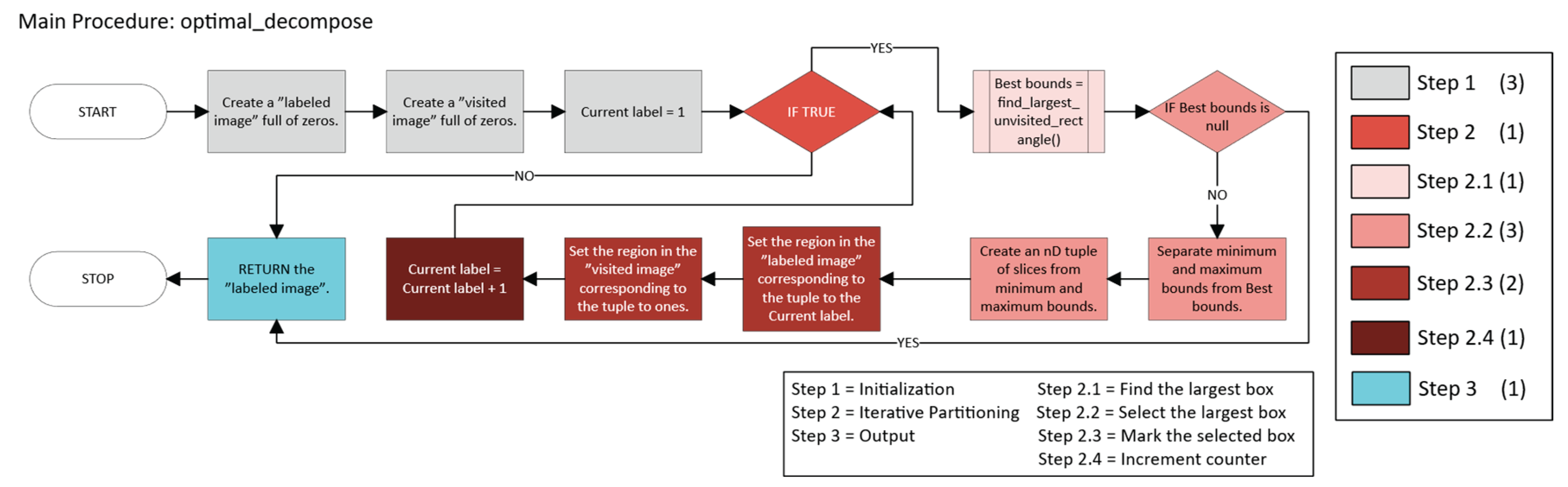
Figure 2.
The find_largest_unvisited_rectangle function of the Python implementation of the pure greedy method.
Figure 2.
The find_largest_unvisited_rectangle function of the Python implementation of the pure greedy method.
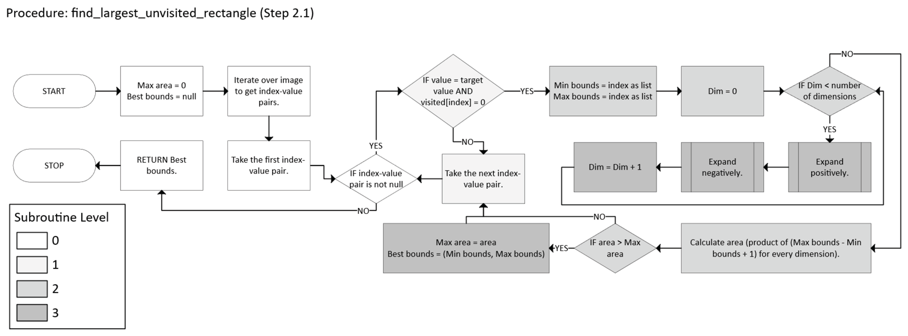
Figure 3.
Expansion subprocesses of the Python implementation of the pure greedy method.
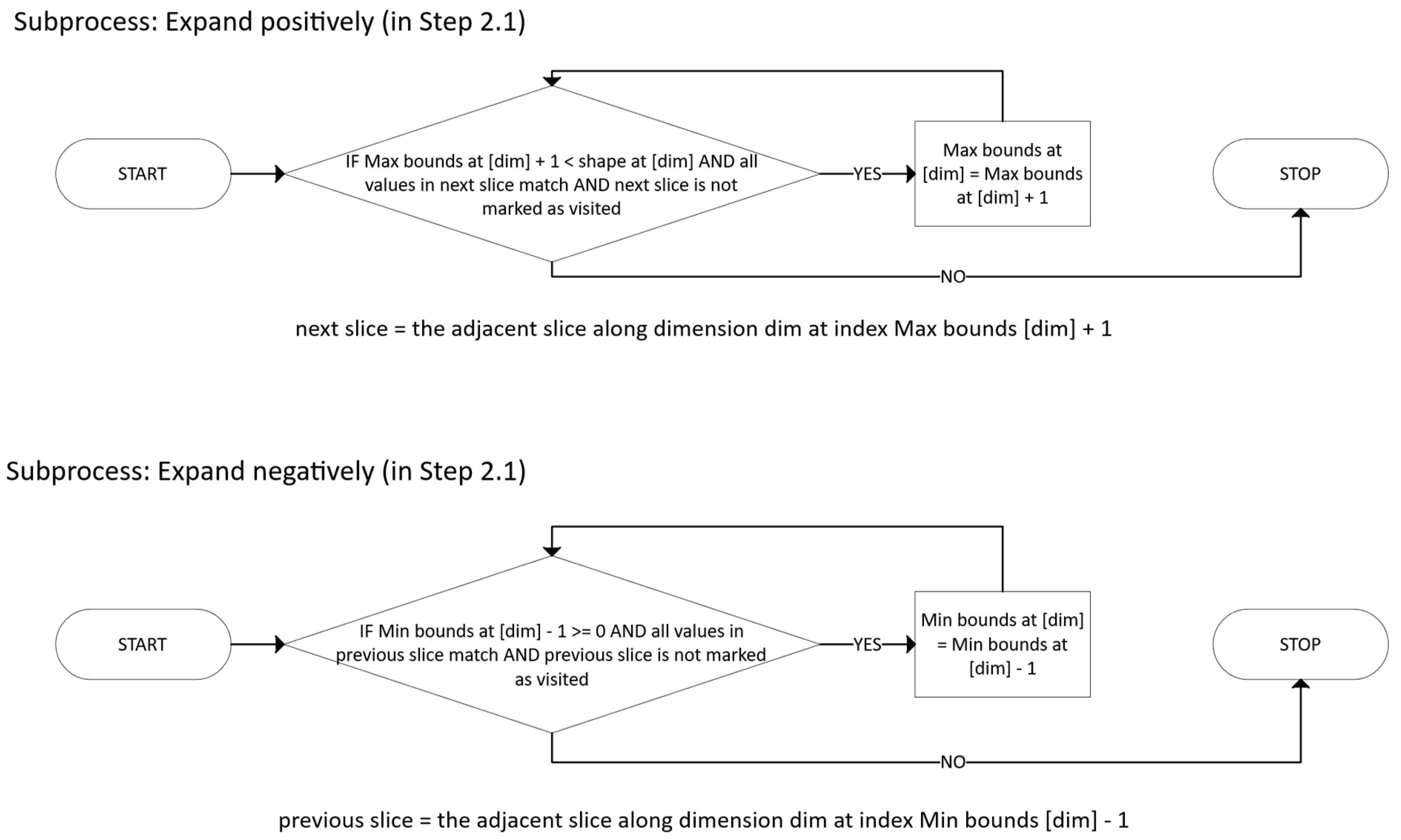
Figure 4.
Top-level chart of the pure greedy method.
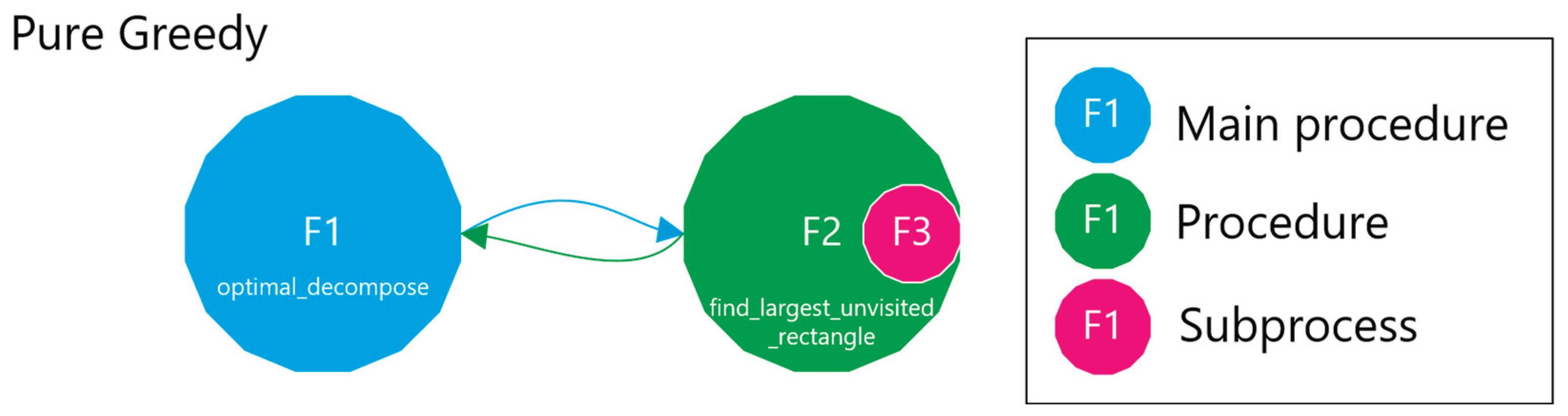
Figure 5.
The main function of the Python implementation of the Greedy BT method.
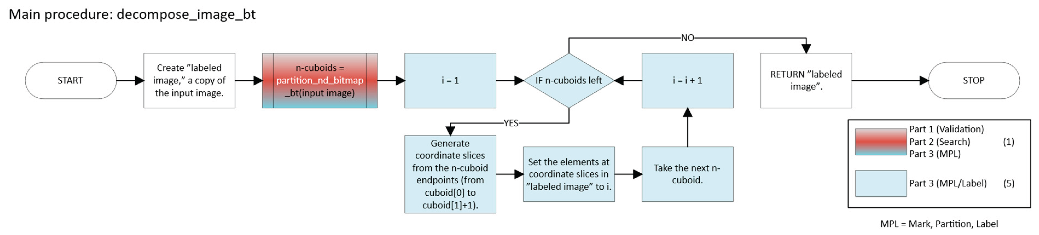
Figure 6.
The partition_nd_bitmap_bt function of the Python implementation of the Greedy BT method.
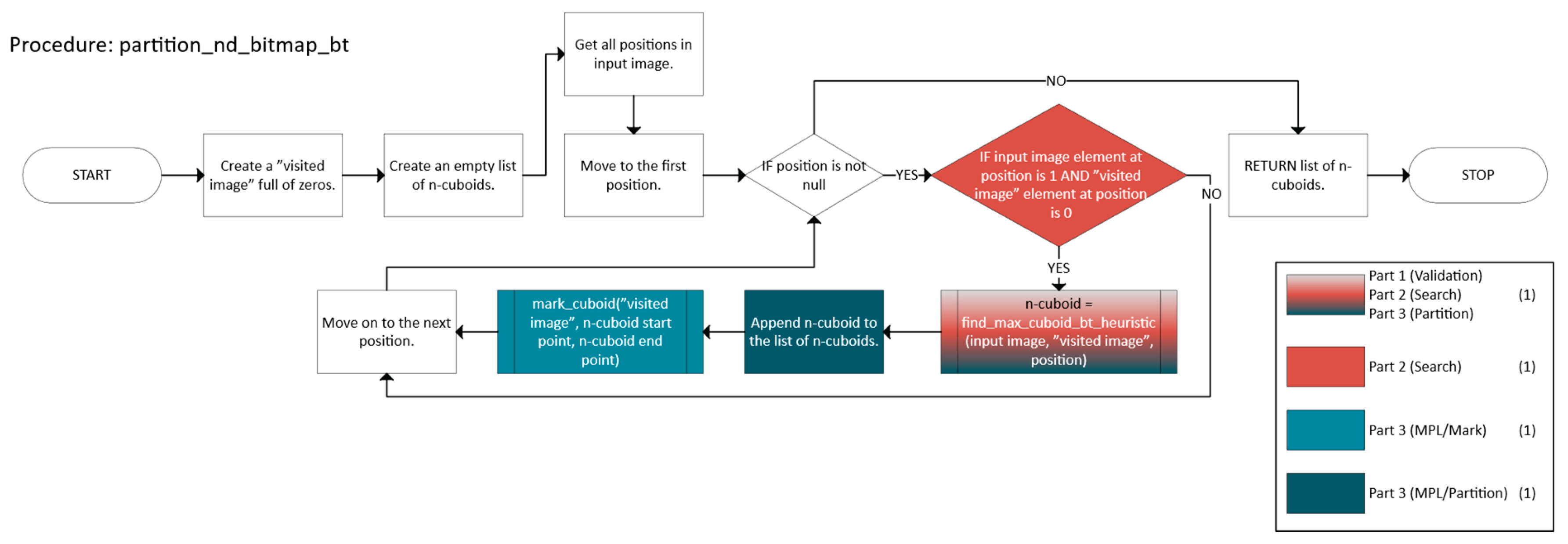
Figure 7.
The mark_cuboid function of the Python implementation of the Greedy BT method.
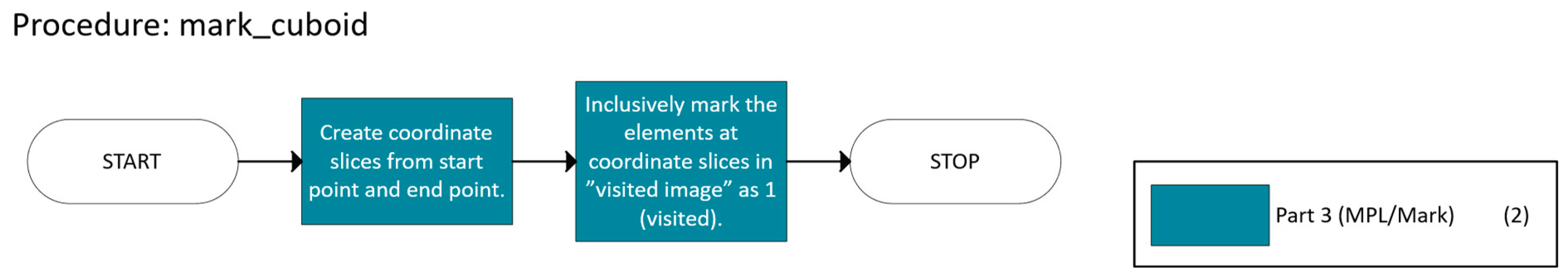
Figure 8.
The find_max_cuboid_bt_heuristic function of the Python implementation of the Greedy BT method.
Figure 8.
The find_max_cuboid_bt_heuristic function of the Python implementation of the Greedy BT method.
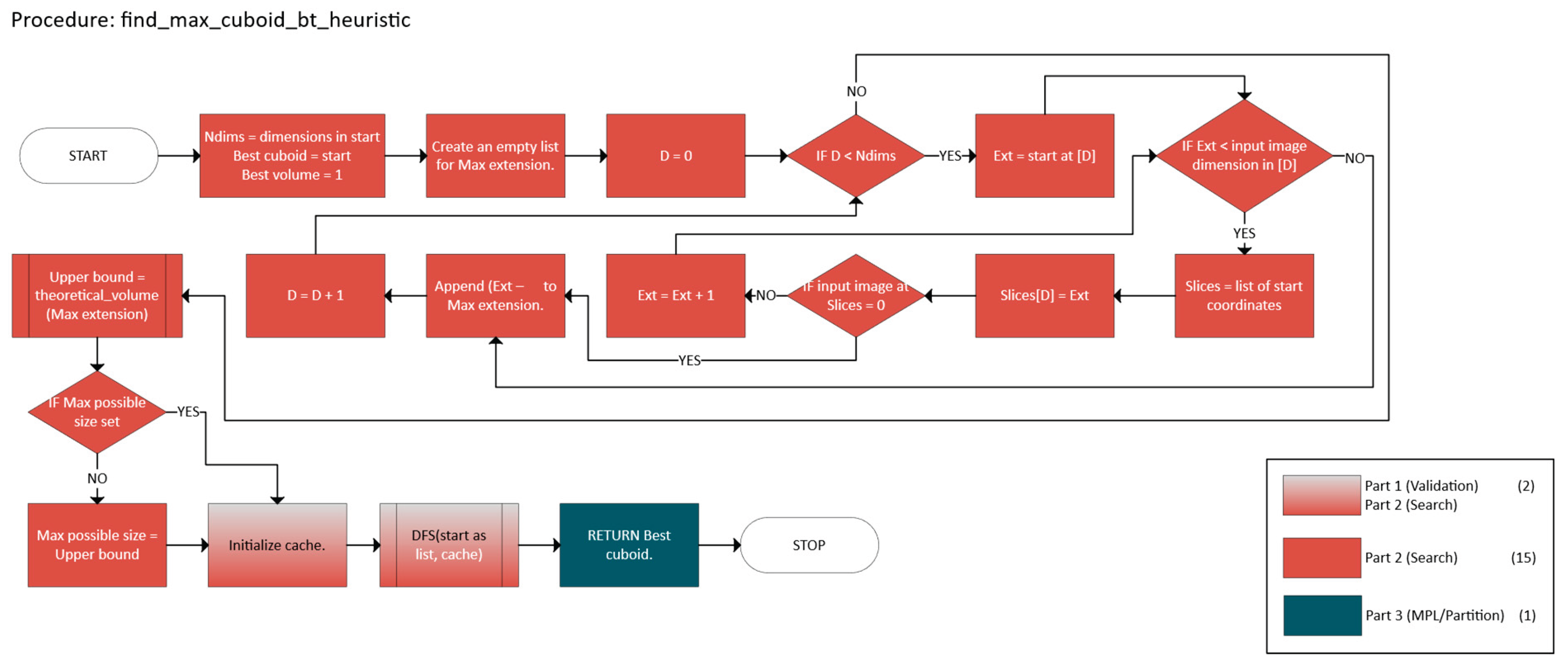
Figure 9.
The theoretical_volume function of the Python implementation of the Greedy BT method.
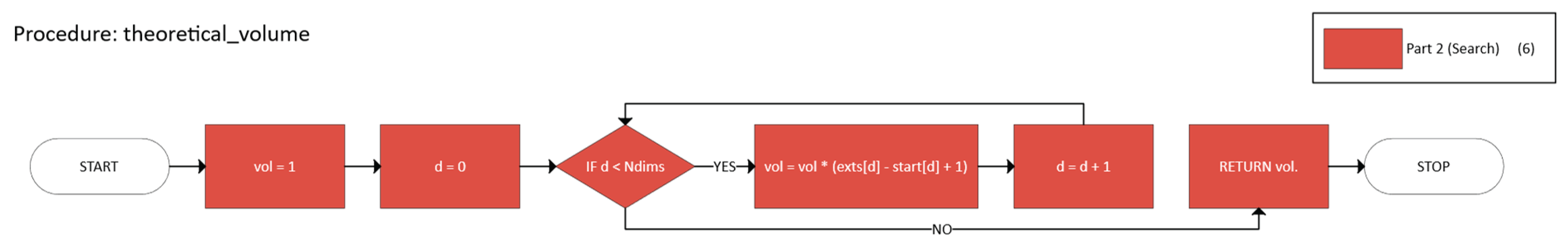
Figure 10.
The volume function of the Python implementation of the Greedy BT method.
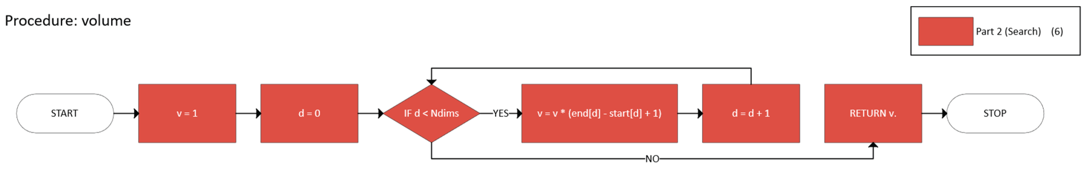
Figure 11.
The DFS (depth-first search) function of the Python implementation of the Greedy BT method.
Figure 11.
The DFS (depth-first search) function of the Python implementation of the Greedy BT method.
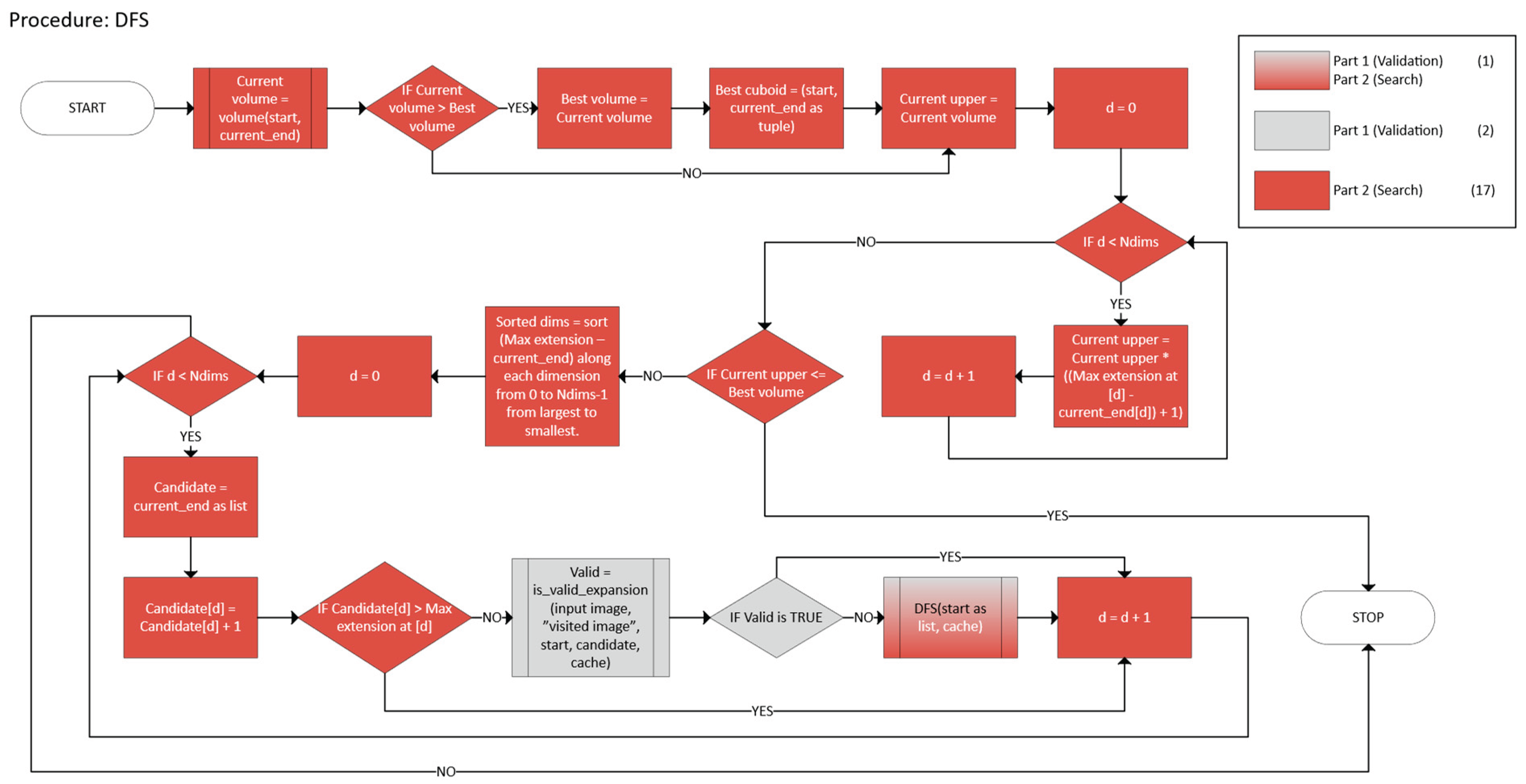
Figure 12.
The is_valid_expansion function of the Python implementation of the Greedy BT method.
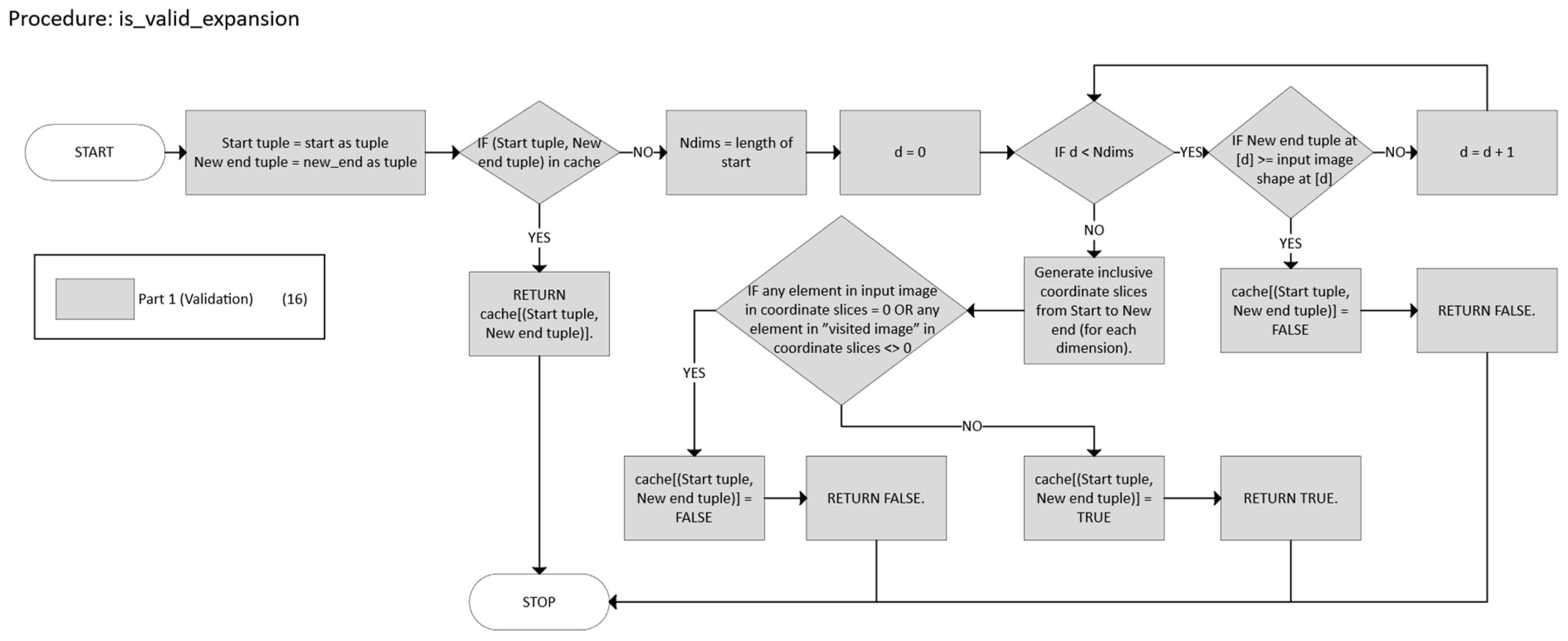
Figure 13.
Top-level chart of the Greedy BT method.
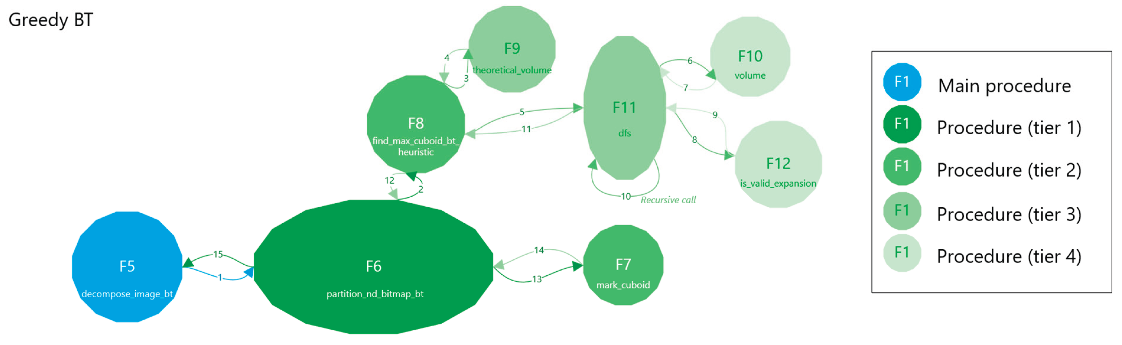
Figure 14.
The main function of the Python implementation of the Greedy PQ method.
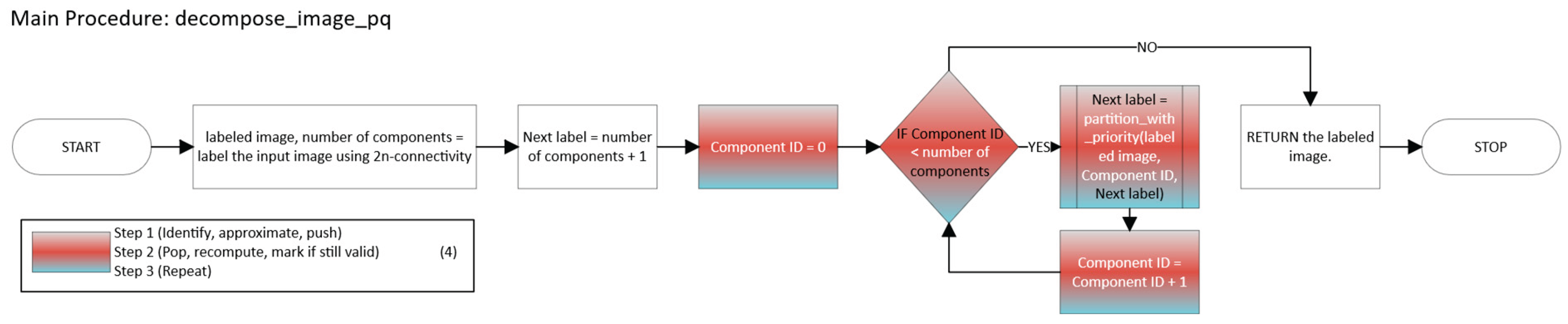
Figure 15.
The partition_with_priority function of the Python implementation of the Greedy PQ method.
Figure 15.
The partition_with_priority function of the Python implementation of the Greedy PQ method.
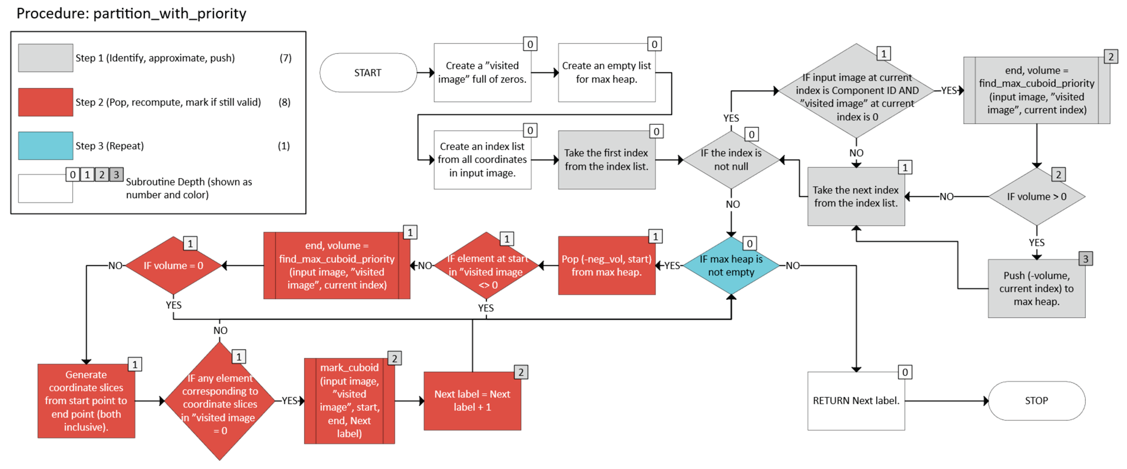
Figure 16.
The mark_cuboid function of the Python implementation of the Greedy PQ method.
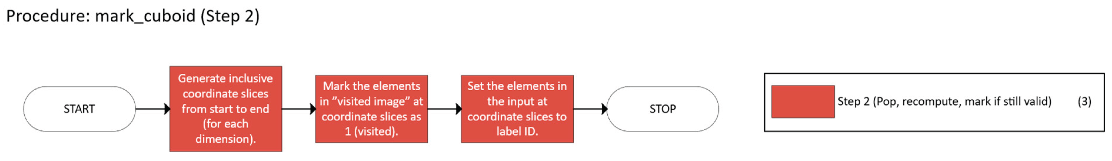
Figure 17.
The find_max_cuboid_priority function of the Python implementation of the Greedy PQ method.
Figure 17.
The find_max_cuboid_priority function of the Python implementation of the Greedy PQ method.
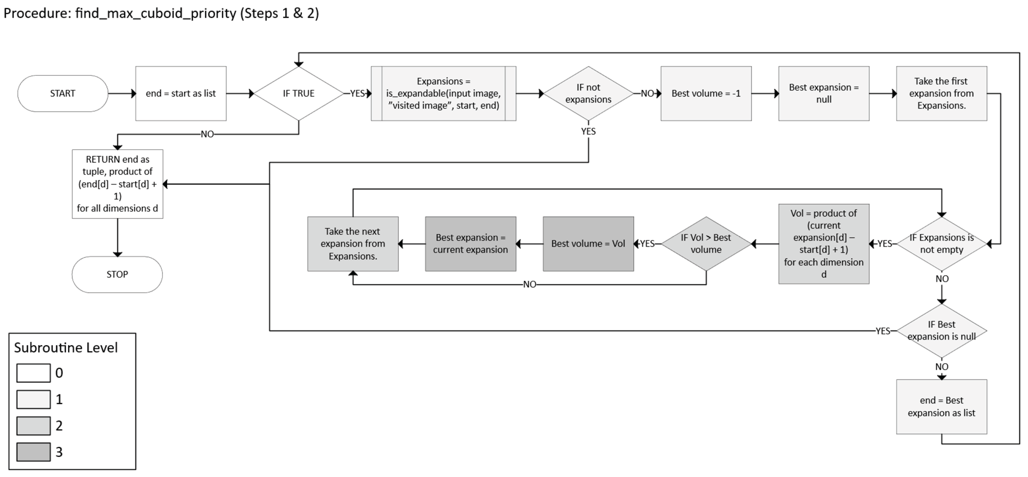
Figure 18.
The is_expandable function of the Python implementation of the Greedy PQ method.
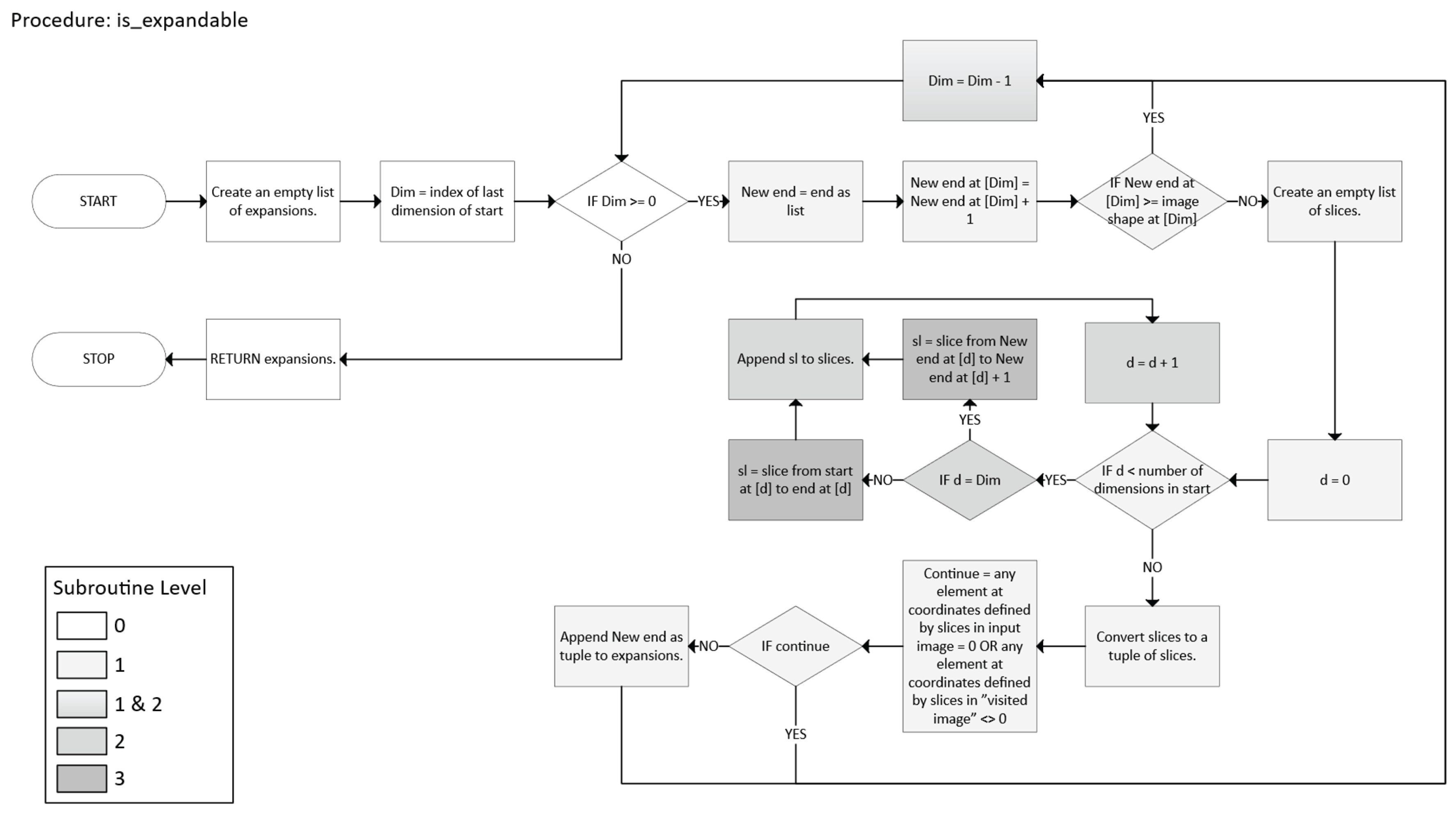
Figure 19.
Top-level chart of the Greedy PQ method.
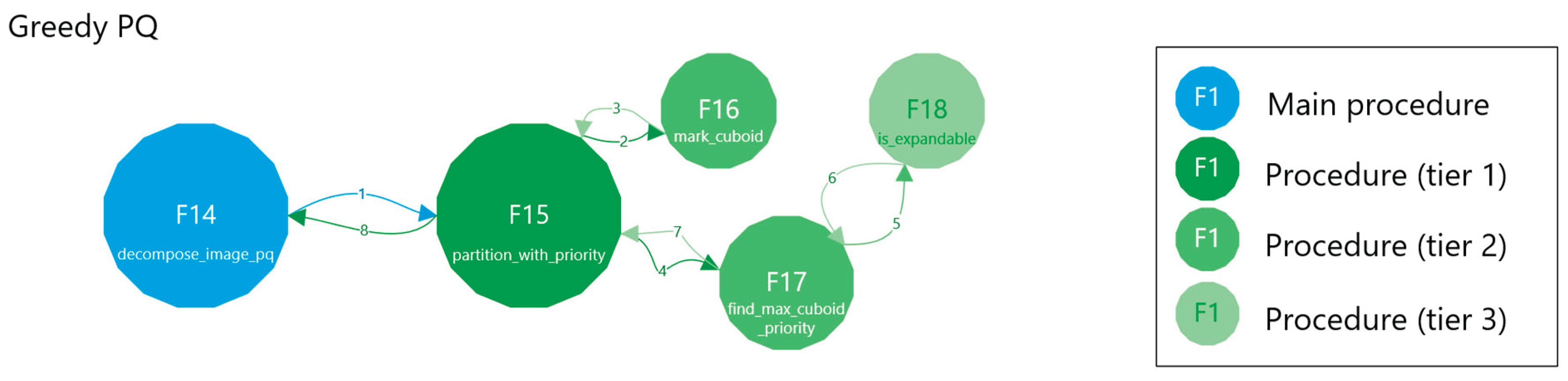
Figure 20.
The main function of the Python implementation of the IILP method.

Figure 21.
The iterative_decomposition function of the Python implementation of the IILP method.
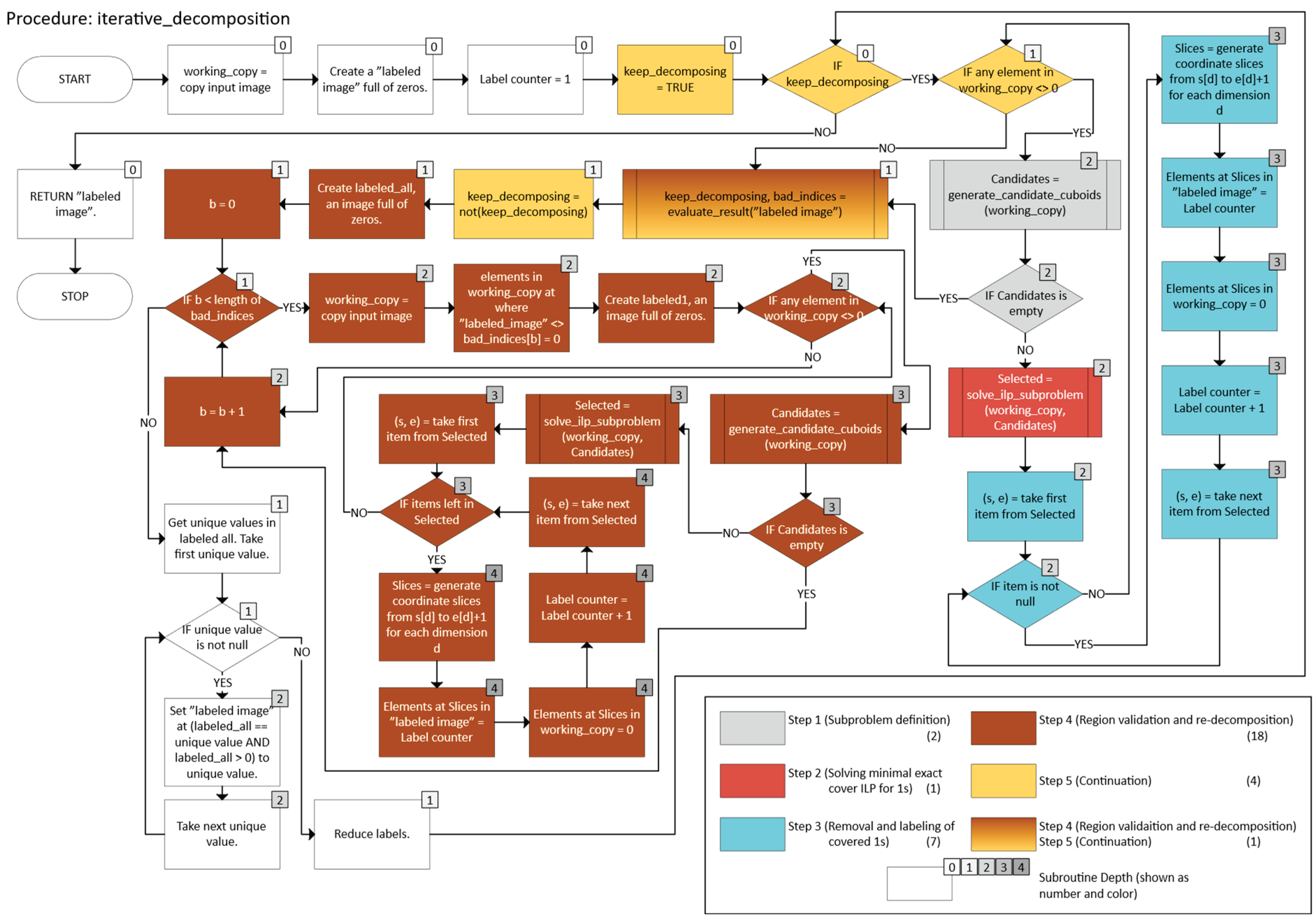
Figure 22.
The evaluate_result function of the Python implementation of the IILP method.
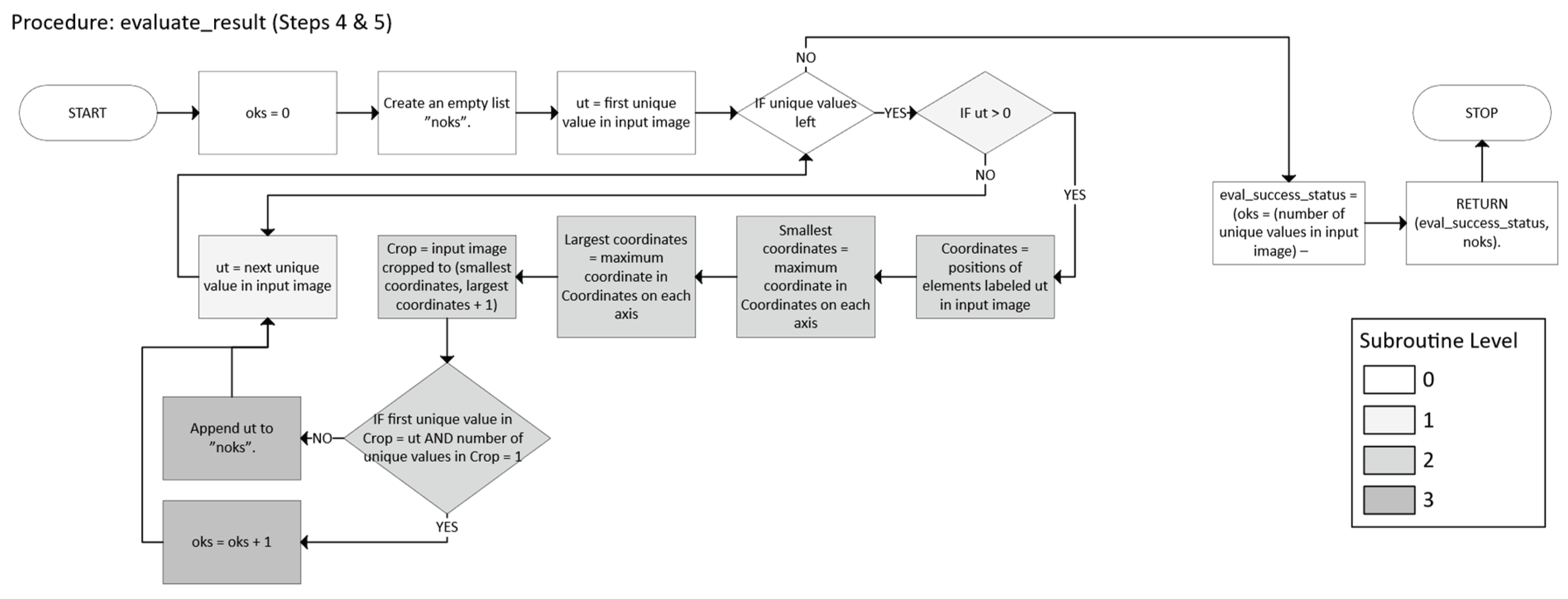
Figure 23.
The function generate_candidate_cuboids of the Python implementation of the IILP method.
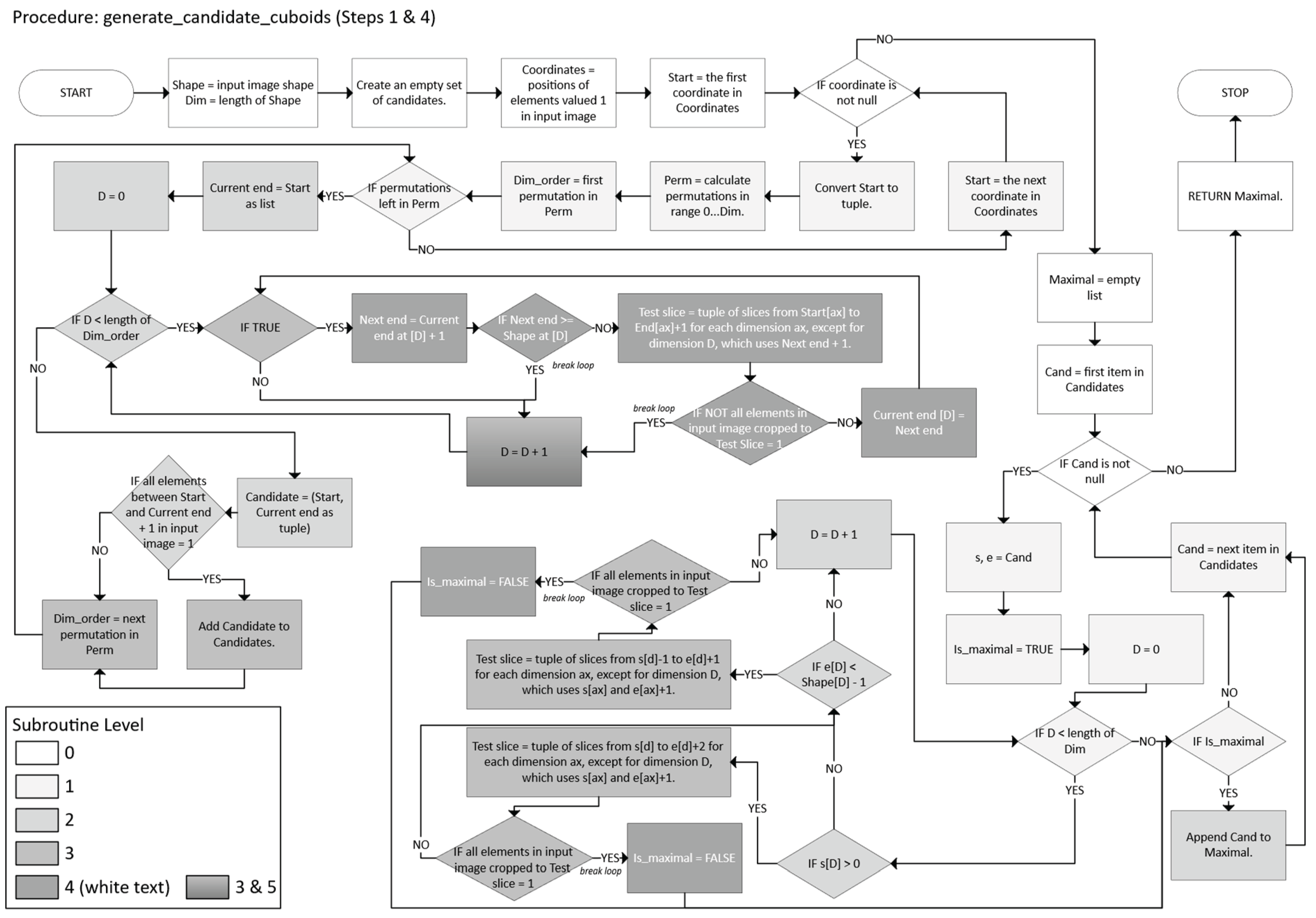
Figure 24.
The solve_ilp_subproblem function of the Python implementation of the IILP method.
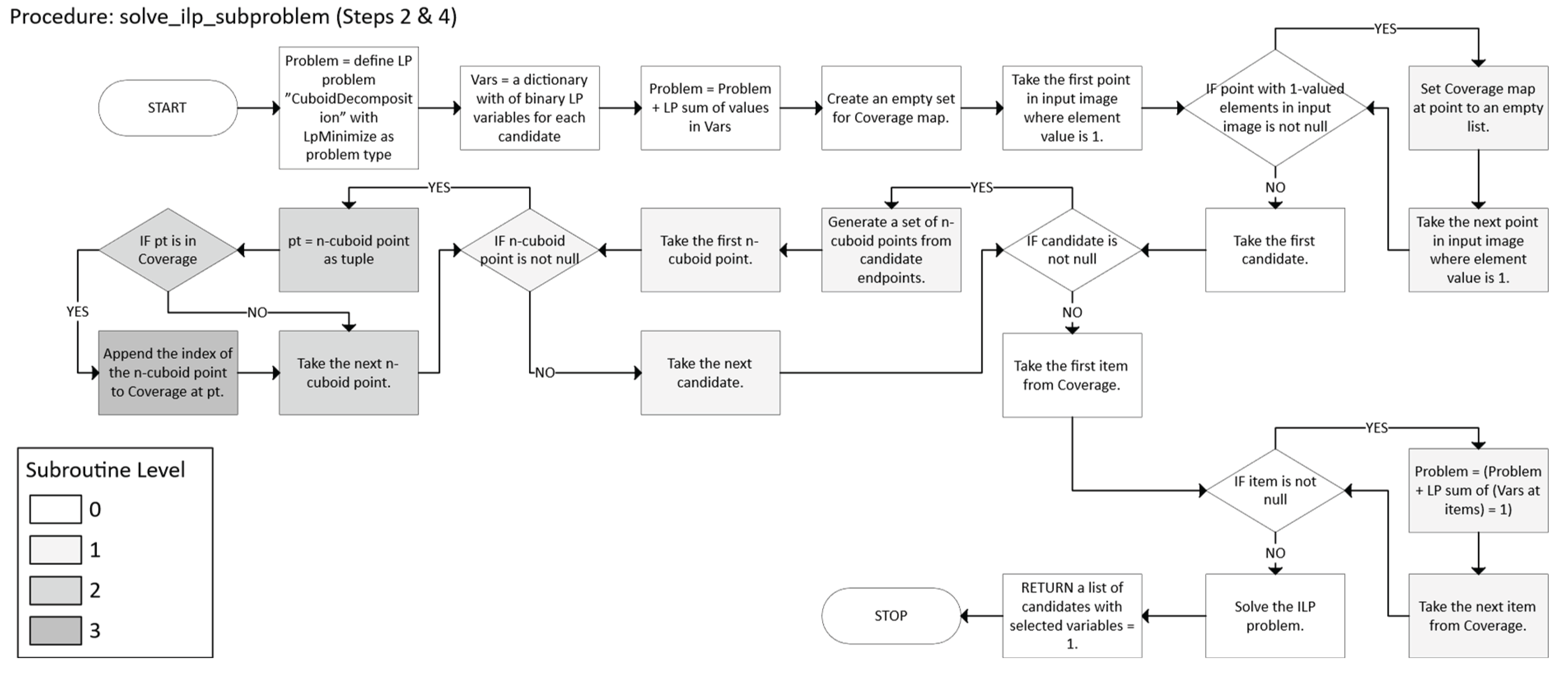
Figure 25.
Top-level chart of the IILP method.
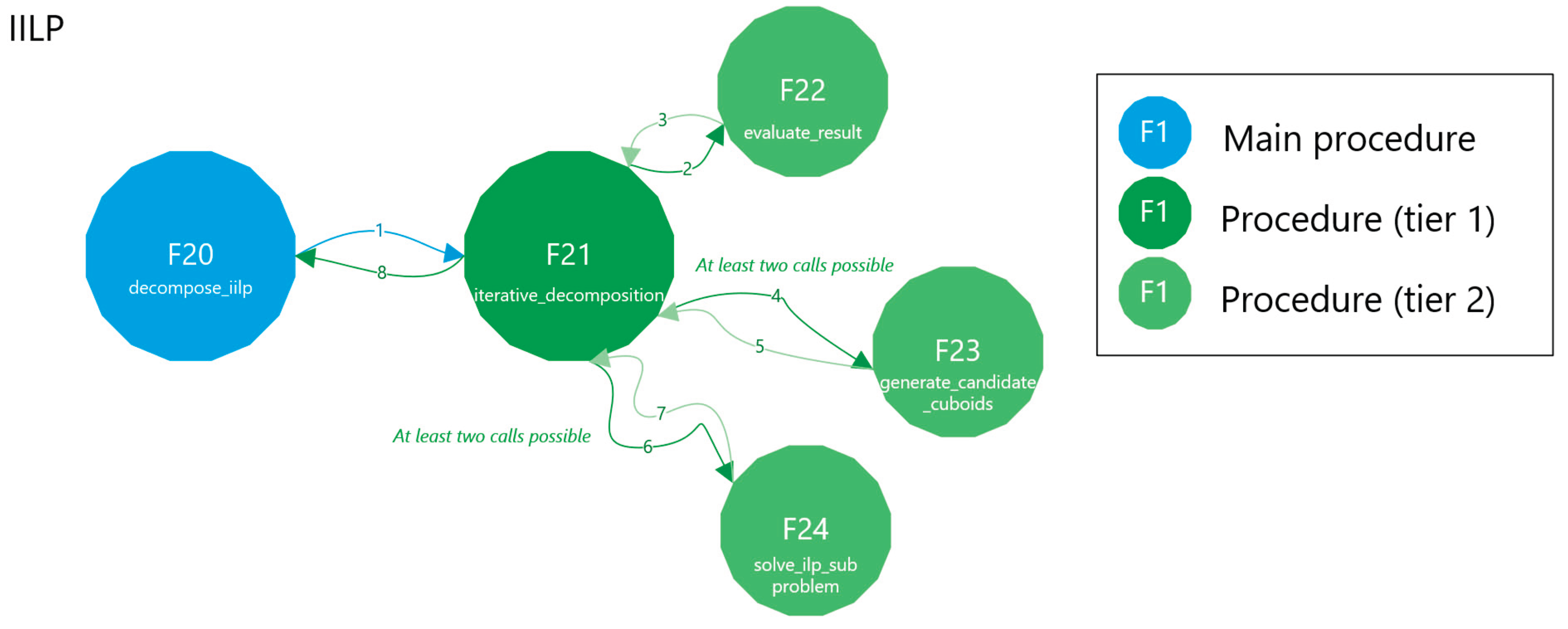
Figure 26.
Two 2D images showing the orientation-sensitivity of the pure greedy method.
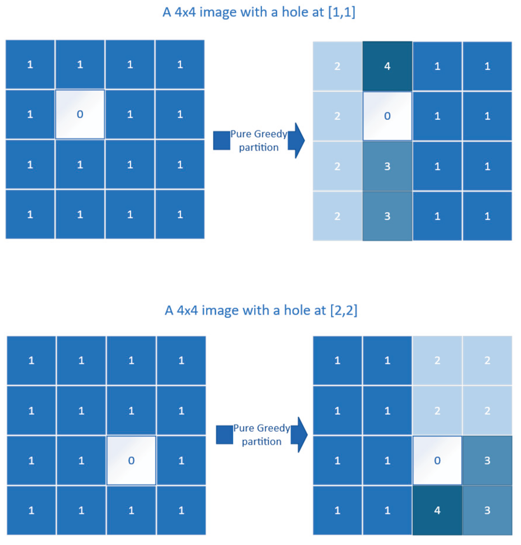

Table 1.
Table 1. The dataset.
| Image | Dimensions | Foreground elements | Description |
|---|---|---|---|
| 9x9x9 | 9×9×9 (3D) | 47.051% | A solid 7×7×7 cube centered in a 9×9×9 image. |
| Holed | 10×10×10 (3D) | 43.2% | A centrally positioned 8×8×8 cube with a 2×2 tunnel passing through its center along all three axes. |
| Holed with Planes YZ | 10×10×10 (3D) | 45.6% | A centrally positioned 8×8×8 cube with a 2×2 tunnel passing through its center only along the Y and Z. |
| Holed with Planes XZ | 10×10×10 (3D) | 45.6% | This is the same as above but with a 2×2 tunnel along the X and Z axes. |
| Holed with Planes XY | 10×10×10 (3D) | 45.6% | This is the same as above but with a 2×2 tunnel along the X and Y axes. |
| Cross3D | 9×9×9 (3D) | 18.519% | A 3×3×3 center with 2-unit-long extrusions in all six directions, forming a 3D cross. The shape is centered in the image. |
| Cross2D | 9×9 (2D) | 40.741% | A 2D version of Cross3D, with a 3×3 center and 2-unit extrusions in four directions. |
| Randomly Generated | 4×4×4 (3D) | 34.375% | A 3D image filled with randomly positioned foreground elements. |
| Steps | 7×7×7 (3D) | 16.035% | A 5×5×5 shape centered in the image, growing from 1×1 to 5×5 in successive slices, forming steps. |
| Squares | 8×8 (2D) | 28.125% | Two 3×3 squares that share one vertex at the center of the image. |
| Cubes | 8×8×8 (3D) | 10.547% | Two 3×3×3 cubes that share one vertex at the center of the image. |
| Hypershape | 8×8×8×8 (4D) | 3.516% | A 4D cross-like shape with a 2×2×2×2 center and 2-unit extrusions along all eight axes. The shape is centered in the image. |
| Lines | 10 (1D) | 50% | A 2-unit and a 3-unit line segment, one starting at the 2nd element from the left, the other at the 2nd element from the right. |
Table 2.
Test results.
| Method | Time | Labels before opt. |
Labels After opt. |
Mean region size before opt. |
Mean region size after opt. |
Reductions | |||||||
| Image 1Box 9x9x9 | Special | 0.0012 | 1.0 | 1.0 | 343.0 | 343.0 | 0.0 | ||||||
| General I | 0.0014 | 1.0 | 1.0 | 343.0 | 343.0 | 0.0 | |||||||
| General II | 0.1547 | 1.0 | 1.0 | 343.0 | 343.0 | 0.0 | |||||||
| Greedy | 0.0755 | 🕐 | 1.0 | 1.0 | 343.0 | 343.0 | 0.0 | ||||||
| Greedy BT | 98.2759 | 1.0 | 1.0 | 343.0 | 343.0 | 0.0 | |||||||
| Greedy PQ | 0.1088 | 1.0 | 1.0 | 343.0 | 343.0 | 1.0 | ➖ | ||||||
| IILP | 0.2157 | 1.0 | 1.0 | 343.0 | 343.0 | 0.0 | |||||||
| Image 2Holed | Special | 0.0131 | 21.0 | 12.0 | 20.6 | 36.0 | 8.0 | ||||||
| General I | 0.0288 | 17.8 | 12.0 | 26.7 | 36.0 | 2.8 | |||||||
| General II | 1.8133 | 15.0 | 15.0 | 28.8 | 28.8 | 0.0 | |||||||
| Greedy | 0.2872 | 12.0 | 12.0 | 36.0 | 36.0 | 0.0 | |||||||
| Greedy BT | 0.0878 | 🕐 | 12.0 | 12.0 | 36.0 | 36.0 | 0.0 | ||||||
| Greedy PQ | 0.1100 | 12.0 | 12.0 | 36.0 | 36.0 | 1.0 | ➖ | ||||||
| IILP | 0.3023 | 12.0 | 12.0 | 36.0 | 36.0 | 0.0 | |||||||
| Image 3Holed with Planes YZ | Special | 0.0104 | 18.0 | 9.0 | 25.3 | 50.7 | 7.0 | ||||||
| General I | 0.0068 | 9.6 | 7.8 | 51.1 | 59.5 | 1.4 | |||||||
| General II | 1.0432 | 10.0 | 9.0 | 45.6 | 50.7 | 1.0 | |||||||
| Greedy | 0.1370 | 6.0 | 🔟 | 6.0 | 1️⃣ | 76.0 | 🔸 | 76.0 | 🔶 | 0.0 | |||
| Greedy BT | 3.1528 | 8.0 | 8.0 | 57.0 | 57.0 | 0.0 | |||||||
| Greedy PQ | 0.0996 | 🕐 | 6.0 | 🔟 | 6.0 | 1️⃣ | 76.0 | 🔸 | 76.0 | 🔶 | 1.0 | ➖ | |
| IILP | 0.4814 | 9.0 | 9.0 | 50.7 | 50.7 | 0.0 | |||||||
| Image 4Holed with Planes XZ | Special | 0.0085 | 18.0 | 8.0 | 25.3 | 57.0 | 7.0 | ||||||
| General I | 0.0050 | 9.2 | 7.2 | 52.4 | 65.9 | 1.6 | |||||||
| General II | 0.8557 | 6.0 | 6.0 | 76.0 | 76.0 | 0.0 | |||||||
| Greedy | 0.1595 | 6.0 | 🔟 | 6.0 | 1️⃣ | 76.0 | 🔸 | 76.0 | 🔶 | 0.0 | |||
| Greedy BT | 3.2481 | 8.0 | 8.0 | 57.0 | 57.0 | 0.0 | |||||||
| Greedy PQ | 0.1185 | 🕐 | 6.0 | 🔟 | 6.0 | 1️⃣ | 76.0 | 🔸 | 76.0 | 🔶 | 1.0 | ➖ | |
| IILP | 0.5899 | 10.0 | 10.0 | 45.6 | 45.6 | 0.0 | |||||||
| Image 5Holed with Planes XY | Special | 0.0043 | 11.0 | 7.0 | 41.5 | 65.1 | 3.0 | ||||||
| General I | 0.0134 | 13.8 | 8.6 | 33.3 | 53.9 | 3.4 | |||||||
| General II | 0.8349 | 6.0 | 6.0 | 76.0 | 76.0 | 0.0 | |||||||
| Greedy | 0.1694 | 6.0 | 🔟 | 6.0 | 1️⃣ | 76.0 | 🔸 | 76.0 | 🔶 | 0.0 | |||
| Greedy BT | 3.4828 | 7.0 | 7.0 | 65.1 | 65.1 | 0.0 | |||||||
| Greedy PQ | 0.1293 | 🕐 | 9.0 | 9.0 | 50.7 | 50.7 | 1.0 | ➖ | |||||
| IILP | 0.7395 | 11.0 | 10.0 | 41.5 | 45.6 | 1.0 | ➖ | ||||||
| Image 6Cross3D | Special | 0.0024 | 5.0 | 5.0 | 27.0 | 27.0 | 0.0 | ||||||
| General I | 0.0030 | 5.0 | 5.0 | 27.0 | 27.0 | 0.0 | |||||||
| General II | 0.3257 | 5.0 | 5.0 | 27.0 | 27.0 | 0.0 | |||||||
| Greedy | 0.0383 | 5.0 | 5.0 | 27.0 | 27.0 | 0.0 | |||||||
| Greedy BT | 0.0122 | 🕐 | 5.0 | 5.0 | 27.0 | 27.0 | 0.0 | ||||||
| Greedy PQ | 0.0233 | 5.0 | 5.0 | 27.0 | 27.0 | 1.0 | ➖ | ||||||
| IILP | 0.2105 | 5.0 | 5.0 | 27.0 | 27.0 | 0.0 | |||||||
| Image 7Cross2D | Special | 0.0010 | 3.0 | 3.0 | 11.0 | 11.0 | 0.0 | ||||||
| General I | 0.0014 | 3.0 | 3.0 | 11.0 | 11.0 | 0.0 | |||||||
| General II | 0.0085 | 3.0 | 3.0 | 11.0 | 11.0 | 0.0 | |||||||
| Greedy | 0.0076 | 3.0 | 3.0 | 11.0 | 11.0 | 0.0 | |||||||
| Greedy BT | 0.0018 | 🕐 | 3.0 | 3.0 | 11.0 | 11.0 | 0.0 | ||||||
| Greedy PQ | 0.0061 | 3.0 | 3.0 | 11.0 | 11.0 | 1.0 | ➖ | ||||||
| IILP | 0.0877 | 3.0 | 3.0 | 11.0 | 11.0 | 0.0 | |||||||
| Image 8Randomly Generated | Special | 0.0147 | 22.0 | 7.0 | 1.0 | 3.1 | 4.0 | ||||||
| General I | 0.0064 | 10.2 | 6.6 | 2.2 | 3.4 | 1.4 | |||||||
| General II | 0.0171 | 10.0 | 9.0 | 2.2 | 2.4 | 1.0 | |||||||
| Greedy | 0.0051 | 6.0 | 6.0 | 3.7 | 3.7 | 0.0 | |||||||
| Greedy BT | 0.0016 | 🕐 | 6.0 | 6.0 | 3.7 | 3.7 | 0.0 | ||||||
| Greedy PQ | 0.0028 | 6.0 | 6.0 | 3.7 | 3.7 | 1.0 | ➖ | ||||||
| IILP | 0.0858 | 6.0 | 6.0 | 3.7 | 3.7 | 0.0 | |||||||
| Image 9Steps | Special | 0.0040 | 9.0 | 9.0 | 6.1 | 6.1 | 0.0 | ||||||
| General I | 0.0059 | 9.4 | 8.6 | 6.0 | 6.4 | 0.4 | |||||||
| General II | 0.1110 | 9.0 | 6.0 | 6.1 | 9.2 | 1.0 | |||||||
| Greedy | 0.0176 | 6.0 | 🔟 | 6.0 | 1️⃣ | 9.2 | 🔸 | 9.2 | 🔶 | 0.0 | |||
| Greedy BT | 0.0045 | 🕐 | 9.0 | 9.0 | 6.1 | 6.1 | 0.0 | ||||||
| Greedy PQ | 0.0110 | 6.0 | 🔟 | 6.0 | 1️⃣ | 9.2 | 🔸 | 9.2 | 🔶 | 1.0 | ➖ | ||
| IILP | 0.2779 | 8.0 | 8.0 | 6.9 | 6.9 | 0.0 | |||||||
| Image 10Squares | Special | 0.0008 | 2.0 | 2.0 | 9.0 | 9.0 | 0.0 | ||||||
| General I | 0.0010 | 2.0 | 2.0 | 9.0 | 9.0 | 0.0 | |||||||
| General II | 0.0045 | 2.0 | 2.0 | 9.0 | 9.0 | 0.0 | |||||||
| Greedy | 0.0041 | 2.0 | 2.0 | 9.0 | 9.0 | 0.0 | |||||||
| Greedy BT | 0.0006 | 🕐 | 2.0 | 2.0 | 9.0 | 9.0 | 0.0 | ||||||
| Greedy PQ | 0.0026 | 2.0 | 2.0 | 9.0 | 9.0 | 2.0 | ➖ | ||||||
| IILP | 0.0448 | 2.0 | 2.0 | 9.0 | 9.0 | 0.0 | |||||||
| Image 11Cubes | Special | 0.0008 | 2.0 | 2.0 | 27.0 | 27.0 | 0.0 | ||||||
| General I | 0.0010 | 2.0 | 2.0 | 27.0 | 27.0 | 0.0 | |||||||
| General II | 0.0710 | 2.0 | 2.0 | 27.0 | 27.0 | 0.0 | |||||||
| Greedy | 0.0105 | 2.0 | 2.0 | 27.0 | 27.0 | 0.0 | |||||||
| Greedy BT | 0.0026 | 🕐 | 2.0 | 2.0 | 27.0 | 27.0 | 0.0 | ||||||
| Greedy PQ | 0.0082 | 2.0 | 2.0 | 27.0 | 27.0 | 2.0 | ➖ | ||||||
| IILP | 0.0595 | 2.0 | 2.0 | 27.0 | 27.0 | 0.0 | |||||||
| Image 12Hypershape | Special | 0.0055 | 7.0 | 7.0 | 20.6 | 20.6 | 0.0 | ||||||
| General I | 0.0056 | 7.0 | 7.0 | 20.6 | 20.6 | 0.0 | |||||||
| General II | 5.2097 | 7.0 | 7.0 | 20.6 | 20.6 | 0.0 | |||||||
| Greedy | 0.0639 | 7.0 | 7.0 | 20.6 | 20.6 | 0.0 | |||||||
| Greedy BT | 0.0068 | 🕐 | 7.0 | 7.0 | 20.6 | 20.6 | 0.0 | ||||||
| Greedy PQ | 0.0307 | 7.0 | 7.0 | 20.6 | 20.6 | 1.0 | ➖ | ||||||
| IILP | 0.4979 | 7.0 | 7.0 | 20.6 | 20.6 | 0.0 | |||||||
| Image 13Lines | Special | 0.0008 | 2.0 | 2.0 | 2.5 | 2.5 | 0.0 | ||||||
| General I | 0.0002 | 2.0 | 2.0 | 2.5 | 2.5 | 0.0 | |||||||
| General II | 0.0006 | 2.0 | 2.0 | 2.5 | 2.5 | 0.0 | |||||||
| Greedy | 0.0004 | 🕐 | 2.0 | 2.0 | 2.5 | 2.5 | 0.0 | ||||||
| Greedy BT | 0.0006 | 2.0 | 2.0 | 2.5 | 2.5 | 0.0 | |||||||
| Greedy PQ | 0.0006 | 2.0 | 2.0 | 2.5 | 2.5 | 2.0 | ➖ | ||||||
| IILP | 0.0408 | 2.0 | 2.0 | 2.5 | 2.5 | 0.0 | |||||||
Disclaimer/Publisher’s Note: The statements, opinions and data contained in all publications are solely those of the individual author(s) and contributor(s) and not of MDPI and/or the editor(s). MDPI and/or the editor(s) disclaim responsibility for any injury to people or property resulting from any ideas, methods, instructions or products referred to in the content. |
© 2025 by the authors. Licensee MDPI, Basel, Switzerland. This article is an open access article distributed under the terms and conditions of the Creative Commons Attribution (CC BY) license (http://creativecommons.org/licenses/by/4.0/).
Copyright: This open access article is published under a Creative Commons CC BY 4.0 license, which permit the free download, distribution, and reuse, provided that the author and preprint are cited in any reuse.


