
Submitted:
23 June 2025
Posted:
23 June 2025
You are already at the latest version
Abstract
The primary distinction between technical design and engineering design lies in the role of analysis and optimization. From its inception, descriptive geometry has supported military and engineering applications, and its graphical rules inherently reflect principles of optimization—similar to the core ideas of sparse representation and compressed sensing. This paper explores the geometric and mathematical significance of the center line in symmetrical objects and the axis of rotation in solids of revolution, framing these elements within the theory of sparse representation. It further establishes rigorous correspondences between geometric primitives—points, lines, planes, and symmetric solids—and their sparse representations in descriptive geometry. By re-examining traditional engineering drawing techniques from the perspective of optimization analysis, this study reveals the hidden mathematical logic embedded in geometric constructions. The findings not only support deeper integration of mathematical reasoning in engineering education but also provide an intuitive framework for teaching abstract concepts such as sparsity and signal reconstruction. This work contributes to interdisciplinary understanding between descriptive geometry, mathematical modeling, and engineering pedagogy.
Keywords:
Descriptive geometry
; Sparse representation
; Compressed sensing
; Optimization analysis
; Mathematical modeling
1. Introduction
Descriptive geometry is often regarded as the foundation of engineering drawing, which in turn serves as a tool for expressing engineering designs in fields such as mechanical and architectural engineering. In descriptive geometry, the theory of affine transformation within parallel projection provides the basis for solving geometric problems using the method of changing planes. The aim of the plane-change method is to position the figure in a special orientation relative to the projection plane, allowing the capture of the true shape characteristics of the object. When a figure is in such a special orientation, the corresponding vector expression becomes a sparse representation of the figure’s data. In engineering drawing, the methods of representation such as sectional views, oblique views, partial views, and oblique sectional views correspond to projection planes that greatly exceed the number of basis vectors required in three-dimensional space. This constitutes a form of redundant representation. Such redundancy is precisely the necessary condition that enables sparse representation and compressed sensing.
The National Center for Engineering and Technology Education (NCETE) has distilled the core concepts of engineering design into constraints, optimisation, and predictive analysis [1] (COPA). Engineering concepts involve numerous factors, including function, structure, materials, aesthetics, cost, process, ethics, mathematics, physics, chemistry, and information. Sparse and optimisation theories are vital means of considering all these factors comprehensively. As a fundamental course in engineering, the theory of descriptive geometry and engineering drawing consistently reflects this engineering mindset and optimisation theory.
The foundation of Descriptive Geometry lies in Orthographical theory, which describes the geometric elements of spatial objects and their projection on the plane as affine transformations. The broader theory of projective transformations encompasses both parallel and central projection theories, and when extended to N-dimensional space, it forms the basis of big data analysis [15]. For instance, a recent doctoral thesis published in 2024 [16] by EPFL (École polytechnique fédérale de Lausanne) directly integrates projective geometry with deep learning. Recent research hotspots such as compressed sensing and sparse representation theory can also be understood as applications of projective theory. Since affine transformation is a special case of projective transformation, orthographical theory is a specific instance of projective theory. Compressed sensing and deep learning theories can be derived from the foundation of projective theory [2], and under certain conditions, compressed sensing theory can be deduced from orthographical theory.
It is well known that the mathematical foundations of compressed sensing and deep learning include optimisation theory, matrix analysis, algebraic geometry, and so on. Matrix analysis and algebraic geometry often analyse artificial intelligence theory from the perspective of algebraic structures (transformation groups), which can be obscure and difficult to understand for engineering students. Most engineering students need to study "Descriptive Geometry and Engineering Drawing". Descriptive geometry studies projection theories, including parallel projection and central projection theories, where parallel projection further includes oblique projection and orthographic projection. For multi-parallel projection theory, the mapping relationship between projections of 3D objects in space on projection planes is expressed as an affine transformation [3]. As previously mentioned, an affine transformation is a special case of a projective transformation. In the context of parallel projection theory, its projection characteristics include the invariance of parallelism in line projections, the invariance of the incidence between points and lines, and the invariance of the cross ratio. Under specific conditions, the projection of a line can exhibit properties of convergence and the characteristic of reflecting the true length of the line. These properties provide us with very intuitive tools for understanding compressed sensing and deep learning, which is also the initial motivation for our research into the compressed sensing theory behind descriptive geometry and engineering drawing.
2. Sparse and Redundant Representations in Orthographical Theory
The theory of sparse representation [5] is developed on the foundation of compressed sensing theory.
where represents the original data, is the dictionary, denotes the codes, M is the feature dimension of the data, L represents the number of samples, and N is the size of the dictionary.
In the theory of sparse representation, the atoms (column vectors) in the dictionary D correspond to the three projection axis vectors in the theory of descriptive geometry’s orthographic projection. X represents the projection values of geometric elements on the axis vectors, while Y corresponds to the vectors describing the graphical elements. If the dictionary contains only the three coordinate axis vectors, it is impossible to achieve a sparse representation of the figures beyond points on the axes and lines parallel to the axes [4].
Consider the following issues in descriptive geometry and engineering drawing:
(1) The relationship between the positioning of three-dimensional objects in the three projection planes system and their sparse representation.
As shown in Figure 1, there are two ways of expressing the three views of the same cuboid. Both methods clearly convey the shape and true form of the cuboid. Textbooks usually do not provide rules for the placement of three-dimensional objects, yet almost all adopt the approach shown in Figure 1b, referred to as Scheme B. The reason is straightforward: it is simpler to draw and easier to measure because Scheme B directly reflects the graphical features. Suppose the length, width, and height of the cuboid in the figure are a, b, and c, respectively. If the line segments in the figure are represented by vectors, the line segment parallel to the X-axis can be expressed as , the line segment parallel to the Y-axis as , and the line segment parallel to the Z-axis as . Sparsity refers to the number of non-zero elements in a vector; the fewer the non-zero elements, the higher the sparsity. Clearly, Scheme B in Figure 1 better meets the sparsity requirements compared to Scheme A.
(2) Dimensioning and sparsity representation.
As shown in Figure 2, a rectangular notch is cut out along the hypotenuse of a triangular area. When marking the dimensions of this figure, the majority of people would opt for Scheme A, while some beginners might choose Scheme B. Typically, we consider Scheme A to introduce an engineering mindset, which aligns well with the theory of sparse representation. Both dimensioning schemes can uniquely determine the shape and size of the figure, but the dimensions in Scheme A are oriented in four directions, whereas those in Scheme B are only in two directions. From vector analysis theory, we know that two independent vectors in two-dimensional space can serve as the basis vectors for the two-dimensional vector space. Although Scheme B’s dimensions are limited to two directions, they are sufficient to clearly express the size and shape of the figure. Scheme A, with its four directional dimensions, may have redundancy, but it provides clarity. This clarity arises because the dimensions in Scheme A align with the characteristic directions of the figure, and the notation reflects the shape features of the figure. This is the fundamental reason for the existence of the sparse representation theory.
(3) Symmetry Centre Line, Axis of Rotation, and Sparse Representation
In descriptive geometry and engineering drawing, it is necessary to draw the symmetry centre line of symmetrical figures and the axis of rotation corresponding to the projection of rotational bodies, as they represent the features of the figures. In symmetrical figures, the two parts symmetrical to each other can be mapped through mirror transformation relative to the axis of symmetry. According to the theory of affine transformation, the invariant in mirror transformation is the axis of symmetry. The mapping between different generatrices in a surface of revolution is a rotational transformation relative to the axis of rotation. From the geometric meaning of the eigenvectors of a matrix, it is known that the symmetry centre line corresponds to the eigenvector of the mirror transformation matrix, and the axis of rotation corresponds to the eigenvector of the rotational transformation matrix. In reverse engineering, how can one determine whether a geometric shape, represented by point cloud data, possesses symmetrical characteristics? According to the geometric meaning of principal component analysis, it is easy to understand that the eigenvectors of the covariance matrix, which is constructed from the point cloud data of the geometric body, correspond to the centre line or axis of rotation of the shape.
The centre line and axis of rotation correspond to the eigenvectors of symmetrical bodies and rotational bodies, respectively. By converting the centre line and axis of rotation into parallel lines of the projection axis, the shape can be represented in a sparse manner.
(4) Drawing Expression Methods and Sparse Representation
The methods of drawing representation include the six basic views, oblique views, auxiliary views, partial views, full sectional views, half sectional views, partial sectional views, oblique sectional views, sectional views, various standard drawing methods, and simplified drawing methods. As shown in Figure 3, the number of views for the reduction gearbox casing far exceeds the number of basis vectors in three-dimensional space. Clearly, this is a redundant expression. However, redundancy is not superfluous; it is precisely this redundancy that makes the graphical structure of three-dimensional forms more clearly expressed.
In summary, whether in the field of artificial intelligence, deep learning theory, or sparse representation and compressed sensing theory, the essence is the same as the theory of engineering drawing expression. The goal is to achieve the most sparse representation of data by capturing the structural characteristics of the data.
3. The Compressed Sensing Theory of Geometric Elements in Descriptive Geometry
The fundamental concept of compressed sensing theory is the integration of signal acquisition and compression, thereby avoiding the conventional approach in signal processing where the signal is first sampled and then compressed for transmission. The mathematical model of compressed sensing theory can be expressed as follows [6]:
where P is the observation matrix of , , D is the sparse dictionary (sparse basis), is the compressible original signal of length N, is the observed signal of M dimensions, and is the coefficient vector under the sparse basis. In reference [8], it is assumed that the sparse basis D is an orthogonal matrix, which has led many works related to compressed sensing to define D as an orthogonal matrix. In reality, in references [7], M. Elad and D. L. Donoho, among others, have extended the sparse basis to non-orthogonal cases, defining this matrix as a dictionary.
Compared to the Nyquist-Shannon sampling theorem, the sparse dictionary is learned and provides a more accurate representation of the function being approximated relative to the Shannon function. For understanding the sparse dictionary, we can explain it through the projection of points, lines, and planes, for example:
In 3D Euclidean space, although a point has three coordinate values, we can establish a local coordinate system in such a way that the point lies on one of the axes of this local coordinate system. This local coordinate system corresponds to the geometric structure of the point in space (although, strictly speaking, a single point does not constitute a structure; it is merely a special case of a structure). In the global coordinate system, we do not need to measure its position using all three global coordinate axes. A straight line in three-dimensional Euclidean space has a clear and simple geometric structure [9]. A local coordinate system can be established such that one of its axes is parallel or coincides with the straight line, thereby reflecting the geometric structure of the line. For a rectangle, which is characterised by 4 vertices with a total of 12 coordinate values, two axes of the local coordinate system can be aligned or parallel with two adjacent edges of the rectangle. In the local coordinate system, the four points are simply four points on a plane, and the number of non-zero coordinate values is reduced to eight. If we use the relative coordinates between the four characteristic points, the non-zero elements are further reduced to four, or even two (if the origin of the local coordinate system is translated to one of the characteristic points).
Next, we analyse the compressed sensing theory corresponding to geometric elements such as points, lines, planes, and volumes from the perspective of descriptive geometry, including observation matrices and sensing matrices [10].
3.1. The Sparse Representation and Reconstruction Model of Points
As shown in Figure 4, in 3D Euclidean space, let the coordinates of point A be . During the first plane change, the new projection axis passes through the horizontal projection a of point A. In the new projection plane system , point A actually lies on the projection plane . In the second plane change, the new projection axis passes through , and in the newly formed projection plane system , point A lies on the projection axis , with its coordinates expressed as .
The new projection plane system can have infinitely many variations. The simplest form is the projection plane system obtained by translation, where the axis passes through point A, such that the three-projection plane system can still be represented in the form of a unit matrix .
In the theory of compressed sensing, this matrix is referred to as a sparse matrix or a sensing matrix. Professor David L. Donoho from Stanford University suggests that this matrix does not need to be an orthogonal matrix [7], which simplifies our subsequent analysis.
Theorem 1.
A measurement matrix corresponding to a point in 3D Euclidean space allows for the precise reconstruction of the original signal from the measurement signal.
Proof.
Without loss of generality, let the measurement matrix (projection matrix) be denoted as . According to the theory of compressed sensing, as long as the measurement matrix and the vector formed by the three coordinate values of a known point A are not orthogonal, we have:
(1)The measurement signal.
(2) , where is a sparse matrix; x is the original signal, corresponding to a point in 3D Euclidean space; and is the sparse coefficient. Therefore, we have
because
It is evident that by setting , , Equation (4) can be satisfied, and , thereby meeting the sparsity requirement. Next, we use the sparse coefficients obtained in this way to reconstruct the original signal , which represents the coordinates of point A.
According to the original signal reconstruction steps in compressed sensing theory [8], we have:
It is evident that an exact reconstruction of the original signal x has been achieved. Hence, the proof is complete. □
3.2. The Sparsity and Reconstruction Representation of a Straight Line
It should be noted that the signal being processed is a straight line, and a line segment can be determined by two points, which already confirms the sparsity of the signal. In descriptive geometry, to further achieve the sparse representation of a straight line, one can use two plane transformations to convert a general straight line into a line perpendicular to the projection plane, and then by translating the coordinate system so that one of its axes coincides with the line, the maximum sparse representation of the line can be realised. As shown in Figure 5, the line segment MN is a general straight line, which, after two plane transformations, becomes a line perpendicular to the projection plane in the new projection plane system.
For convenience of description, let , , and . Assume that after two changes of the projection plane, in the new projection plane system , the projection axis coincides with the line segment , which can be represented in vector form as ; in the original projection plane system , the corresponding line can be expressed in vector form as . Therefore, the sparse matrix can be defined as
According to compressed sensing theory, the original line signal can be represented using a sparse basis as:
By direct observation, the solution for the sparse coefficient can be obtained as follows: , . We shall not delve into the methods for solving the sparse coefficients at this juncture, but it is important to note that this represents the sparsest solution for the sparse coefficients, .
Next, we present the compressed sensing theorem concerning a line segment in the form of a theorem [11].
Theorem 2.
The measurement matrix corresponding to the line segment formed by two points and in three-dimensional Euclidean space allows for the accurate reconstruction of the original signal from the measured data.
Proof.
Without loss of generality, let the measurement matrix (projection matrix) be
According to the compressed sensing theory, we have:
(1) The measurement signal
(2), where is a sparse matrix; x is the original signal, corresponding to two points in 3D Euclidean space; is the sparse coefficient. Therefore,
because
where
It is not difficult to see from Equation (7) that by choosing , , Equation (6) can be satisfied, and , which meets the sparsification requirement. Using Equation (8), the sparse coefficient can be obtained to reconstruct the original signal . This completes the proof of the theorem.
□
It is easy to understand that in the sensing matrix , the first and fourth column vectors are the most crucial, while the second, third, fifth, and sixth column vectors only need to be uncorrelated with the first and fourth column vectors. For this reason, the observation matrix only needs to retain the information from the first and fourth column vectors, so an observation matrix with 2 rows and 6 columns will suffice to meet the requirements.
For a line segment, another more general vector expression method involves transforming the line segment into a line parallel to the coordinate axes, using a linear combination of the vector formed by the endpoint coordinates and the coordinate axis vectors. As shown in Figure 6, the length of the line segment is , and the red unit vector can be expressed as: , where , , . Its direction is parallel to the line segment .
In this method of representation, the local coordinate axes that make up the perception matrix are parallel to, but do not coincide with, the direction of the known line segment. A straight line segment can be expressed as a vector, , and the corresponding perception matrix is represented as
The sparse expression of the line segment is given by , and its corresponding matrix expression is
According to compressed sensing theory, its sparsest solution can be expressed by the following optimisation formula:
It can be directly observed that , , , , . at first glance, the sparse coefficient vector does not appear sufficiently sparse. However, the matrix possesses a certain degree of generality, enabling it to represent all lines parallel to line , such as the magenta parallel lines shown in Figure 6. Furthermore, when additional points are added on line , the number of non-zero elements in the sparse coefficient vector does not need to increase. For instance, when point C is added on the extension of line AB, making points A, B, and C evenly distributed, the signal containing the three points is still represented.
The sparse expression is , and the corresponding matrix form is
Direct observation reveals that
Similar to the analysis of Theorem 2, the key to the aforementioned sensing matrix lies in the first four column vectors. As long as the observation matrix can capture the first four column vectors of the sensing matrix, it guarantees the accurate reconstruction of the original signal x from the observed signals.
3.3. Sparsity of Planar Polygons
In three-dimensional Euclidean space, a point requires three coordinate values to determine its position; a line segment requires two endpoints, which amounts to 6 coordinate values to define its location. However, when a point in space lies on one of the coordinate axes, only one of its coordinate values is non-zero; similarly, a line segment would have only two non-zero coordinate values. For instance, point A on the X-axis has coordinates ; the line segment on the X-axis has coordinates .
For a planar polygon formed by k characteristic points, the method of plane projection can be employed so that the plane coincides with a projection plane, such as the horizontal projection plane. In this case, the z-coordinates of these k characteristic points are zero, and the vector composed of the coordinate values of these k points is -sparse. As shown in Figure 7, the four characteristic points of a quadrilateral lie on the same plane, forming a vector with 12 elements, of which 4 elements are zero.
In the theory of sparse representation of lines, only one dimension of the three-dimensional coordinate system is utilised, and the other two coordinate axes are effectively redundant. For simplicity, we will directly use planar figures as examples to illustrate the principle of compressed sensing for planar figures with certain geometric structures. As shown in Figure 7, a seemingly complex planar polygon has edges that actually follow only two directions. In the local coordinate system formed by the two red-marked vectors, all contour edges are either horizontal or vertical lines. Compressed sensing theory exploits this particular geometric structure.
As illustrated in Figure 8, the principal components are immediately apparent; however, the structure is not symmetrical. This dataset pertains to planar data, but the principal components should encompass three directions, which can be further extended to additional directions. The model can be described as follows:
Clearly, this is a problem of sparse representation and compressed sensing.
3.4. Sparsity of Solids
Basic solids of revolution (cylinders, cones, spheres) and plane solids with symmetrical properties (prisms and pyramids), despite having numerous lines in their diagrams, can achieve compressed sensing through their axis of symmetry and axis of rotation. It can be demonstrated that the eigenvectors of the covariance matrix, formed by the characteristic points of a solid, correspond to the axis of symmetry or the axis of rotation of the solid. This is the primary reason for performing singular value decomposition on data matrices in sparse representation, compressed sensing, and deep learning [12]. For symmetric geometric bodies involved in descriptive geometry and engineering drawing, the axis of rotation or symmetry can be directly obtained from the eigenvectors of the data matrix.
Store the given m pieces of n-dimensional data in an matrix D, then perform zero-mean normalisation on each row of matrix D. Next, construct the covariance matrix of the dataset and compute its eigenvalues and eigenvectors. Arrange the eigenvectors in a matrix, sorted by their corresponding eigenvalues from largest to smallest. Select the first k rows to form matrix P. By multiplying matrix P with the original dataset matrix, the dimensionally reduced data can be obtained.
If we take the characteristic points that define a line or a plane as a dataset, can we use Principal Component Analysis (PCA) to analyse the principal components of this dataset? Without loss of generality, let us consider the cuboid shown in Figure 9 as an example. The axis of the cuboid (depicted by the blue dashed line) is in a general position with respect to the coordinate system shown. Based on the symmetry of the cuboid’s vertices relative to the midpoint O, it can be deduced that
According to the principles of Principal Component Analysis, the set of points formed by the eight vertices of the cuboid can be represented in the following matrix form:
The covariance matrix corresponding to matrix D is
Matrix C’s eigenvalues can be determined as follows:
To simplify calculations, we employ the method of change plane to transform the central axis of the cuboid (indicated by the blue dashed line) into the vertical line of the projection plane, as shown in Figure 10. Clearly, directly computing the corresponding eigenvalues and eigenvectors is rather challenging.
Without loss of generality, the new projective plane system (purple coordinate axes ) shown in Figure 10 can be easily obtained by selecting the axonometric axes and adopting the method of "changing the plane." The coordinate values of the 8 vertices under the new coordinate system are shown in Figure 10. Let the length, width, and height of this cuboid be 2a, 2b, 2c, respectively, then there are
In the new coordinate system, the set of points formed by the 8 vertices of the cuboid can be represented in the following matrix form:
The covariance matrix corresponding to matrix D’ is
The eigenvalues of a matrix can be determined by the following method:
Hence, it is not difficult to deduce:
Next, we seek the corresponding eigenvectors.
(1)
According to the definition of matrix eigenvectors, we have
Solving equation system (14), we obtain the eigenvalues and their corresponding eigenvectors as follows: the eigenvector corresponding to eigenvalue is ; similarly, we have for and for . These three eigenvectors have clear geometric interpretations, as they correspond to the three purple coordinate axes in Figure 10.
Next, we will use the method of change plane to find the eigenvalues and eigenvectors in the original coordinate system. According to the definition of eigenvalues, for the same point set, the eigenvalues remain unchanged in different coordinate systems.
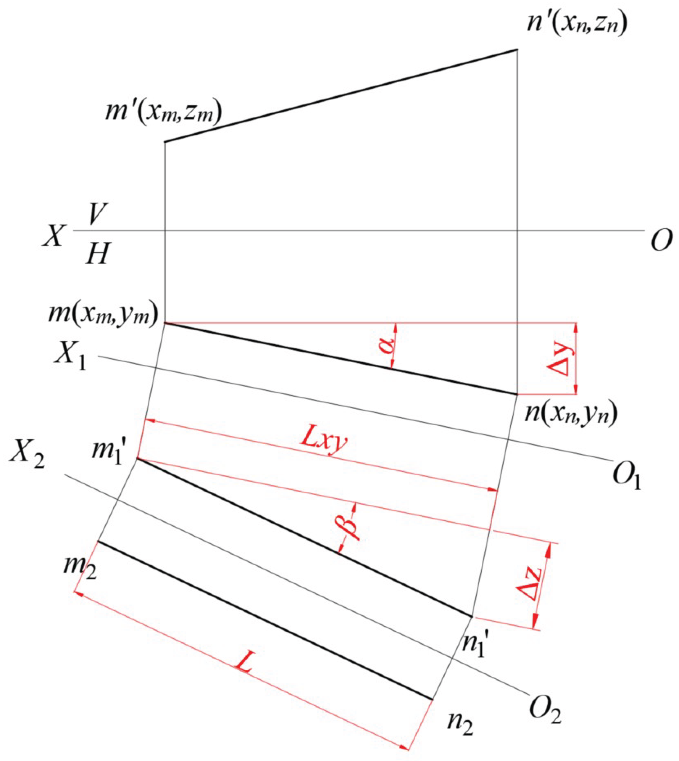
As shown in Figure 11, the vector represents the characteristic vector of the vertex data matrix of the cuboid shown in Figure 10. Without loss of generality, in the new coordinate system (formed by the characteristic vectors of vertices of the symmetrical geometric object), the coordinates of points M and N are (-L/2, , ) and (L/2, , ) respectively. Hence, the coordinates of , as shown in Figure 11, are (-L/2, ), and the coordinates of are (L/2, ). Below, we will transform back the projections and of the line segment MN in the new projection plane system to the original projection plane system [13].
Step one, change the H-plane. Rotate by an angle around the Y-axis.
The first step can be represented by the corresponding rotation transformation matrix as follows.
Step two, change the V-plane. Rotate by an angle around the Z-axis.
Where , the corresponding rotation transformation matrix can be represented as
Step three involves transforming the line segment MN’s projections, and , from the new projection plane system back to the original projection plane system.
The result indicates that, regardless of how a cuboid is rotated, the vectors corresponding to its edges are the eigenvectors of the matrix obtained by multiplying its vertex data matrix with its transposed matrix. Therefore, the geometric interpretation of multiplying the vertex data matrix with its transposed matrix can be explained using the method of changing plane.
Hence, it can be observed that for basic three-dimensional solids with a symmetric structure, the choice of axonometric axis and the results of principal component analysis are consistent
For asymmetrical structures, the corresponding eigenvector (principal component) directions are relatively complex. A combination of clustering and singular value decomposition (such as K-SVD) methods may help identify sparse vectors that can represent the characteristics of the shape.
4. Conclusions
As a foundational course for engineering students, Descriptive Geometry and Engineering Drawing serves as a specialised core subject within engineering disciplines. The knowledge of intelligent systems, information technology, interdisciplinary studies, and innovation is essential for engineering students. Interdisciplinarity is a requirement for talent development driven by technological advancement. Professors Persi Diaconis and David Freedman had already posited in the 1980s that graphical projection is the cornerstone of big data analysis [14], yet there is scarcely any literature today that connects Descriptive Geometry with Artificial Intelligence.
This paper focuses solely on the intrinsic connection between the parallel projection method in Descriptive Geometry and sparse representation, as well as compressed sensing. The central projection method, based on projective transformations, has been widely applied in computer graphics and computer vision. The doctoral thesis "Incorporating Projective Geometry into Deep Learning," [16] published by the Swiss Federal Institute of Technology Lausanne in 2024, attempts to integrate projective geometry into deep learning, marking a new development in the field of computer vision. Geometric deep learning theory, on the other hand, dissects the mechanisms of deep learning from the perspective of algebraic geometry. Establishing more fundamental connections between Descriptive Geometry and Artificial Intelligence remains an area with much work to be done.
We established sparse representation and compressed sensing for points, lines, planes, and basic symmetrical solids. However, rotational bodies with asymmetrical structures (such as truncated cylinders and truncated cones) cannot have their rotational axis position expressed through the eigenvectors of the covariance matrix corresponding to the coordinates of feature points. Further research is required to analyse the intrinsic connections between these structures through clustering and singular value decomposition. Other mathematical concepts inherent in Descriptive Geometry, such as shadows and complex numbers, the concept of biorthogonality in double orthogonal projections, and the calculus principles implicit in regular polygon labelling, hold significant importance in establishing internal connections between abstract algebraic knowledge and Descriptive Geometry. These connections are crucial for deeply understanding the mathematical mechanisms of Artificial Intelligence, achieving interdisciplinary integration, and cultivating students’ innovative thinking.
Funding
This research was funded by the Education and Teaching Reform Research Project of China Agricultural University (BZY2023046),the Beijing Higher Education Society under General Research Project (MS2024415), and the National Natural Science Foundation of China (61871380).
Acknowledgments
The author appreciate the constructive feedback and discussions from colleagues.
Conflicts of Interest
The authors declare no conflicts of interest.
References
- Todd R. Kelley. Optimization, an important stage of engineering design. The Technology Teacher 2010, 69, 18.
- Michael Elad. Optimized Projections for Compressed Sensing. IEEE Transactions on Signal Processing 2007, 55(12), 5695–5702. [Google Scholar] [CrossRef]
- He Yuanjun. A New Interpretation of Descriptive Geometry. Journal of Graphics 2018, 39(01), 136–147. [Google Scholar]
- He Yuanjun. Graphics and Geometry. Journal of Graphics 2016, 37(06), 741–753. [Google Scholar]
- Aharon Michal;Michael Elad; Bruckstein Alfred. K-SVD: An algorithm for designing overcomplete dictionaries for sparse representation. IEEE Transactions on signal processing 2006, 54, 4311–4322. [CrossRef]
- David L. Donoho. For most large underdetermined systems of linear equations the minimal L1-norm solution is also the sparsest solution. Communications on Pure and Applied Mathematics: A Journal Issued by the Courant Institute of Mathematical Sciences 2006, 59, 797–829. [CrossRef]
- David L. Donoho, Elad Michael. Optimally sparse representation in general (nonorthogonal) dictionaries via L1 minimization. Proceedings of the National Academy of Sciences 2003, 100, 2197–2202. [CrossRef] [PubMed]
- Emmanuel, J. Candès,Michael B. Wakin. An introduction to compressive sampling. IEEE signal processing magazine 2008, 25(02), 21–30. [Google Scholar]
- Wohlberg Brendt. Efficient algorithms for convolutional sparse representations. IEEE signal processing magazine 2015, 25(01), 301–315. [Google Scholar]
- Schwartz Richard Evan,Tabachnikov Serge. Elementary surprises in projective geometry. Math Intelligencer 2010, 32, 31–34. [Google Scholar] [CrossRef]
- Jin Yingji, Li Yuewu. The Father of Descriptive Geometry – Monge. Mathematical Bulletin 2008, 03, 56–58. [Google Scholar]
- Udo Hertrich-Jeromin. The surfaces capable of division into infinitesimal squares by their curves of curvature:A nonstandard-analysis approach to classical differential geometry. Mathematical Intelligencer 2000, 22, 54–61. [Google Scholar] [CrossRef]
- Mukherjee Rajib. Visual Evaluation of a Geometric Series: Sum of Reciprocals of Odd Powers of Two. Mathematical Intelligencer 2022, 44(1). [CrossRef]
- Diaconis Persi,Freedman David. Asymptotics of graphical projection pursuit. The annals of statistics 1984, 793–815. [Google Scholar]
- Richard Radke; Peter Ramadge; Tomio Echigo; Shun-ichi Iisaku. Efficiently estimating projective transformations. In Proceedings 2000 International Conference on Image Processing (Cat. No. 00CH37101), Vancouver Convention & Exposition Centre, Vancouver, British Columbia, Canada,10-13,September,2000.
- Michal Jan Tyszkiewicz. Incorporating Projective Geometry into Deep Learning. doctoral thesis, École Polytechnique Fédérale de Lausanne, Lausanne, Switzerland, Jan 12,2024.
Figure 1.
Two schemes for expressing the three views of a cuboid.
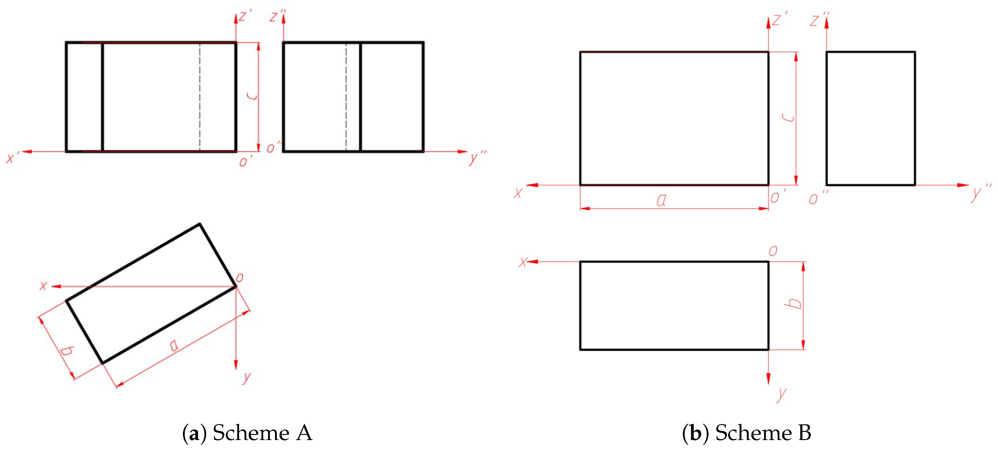
Figure 2.
Two schemes for expressing the three views of a cuboid.
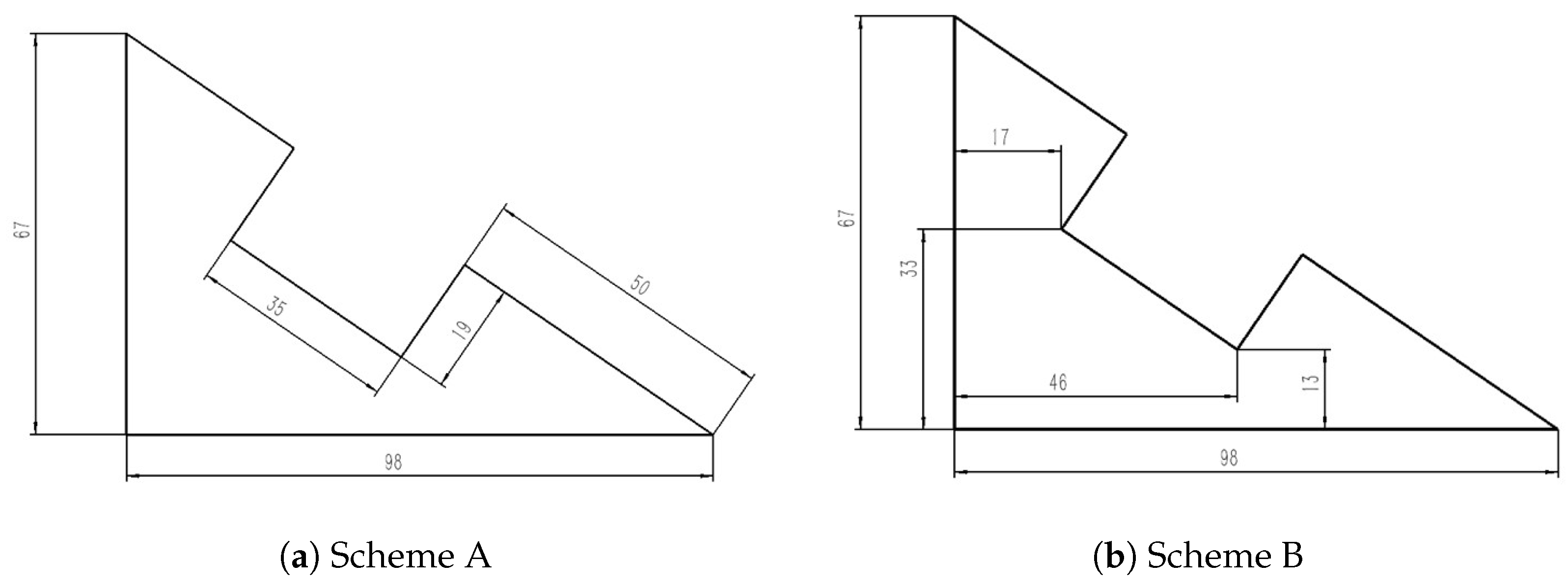
Figure 3.
The view representation of the reduction gearbox housing.
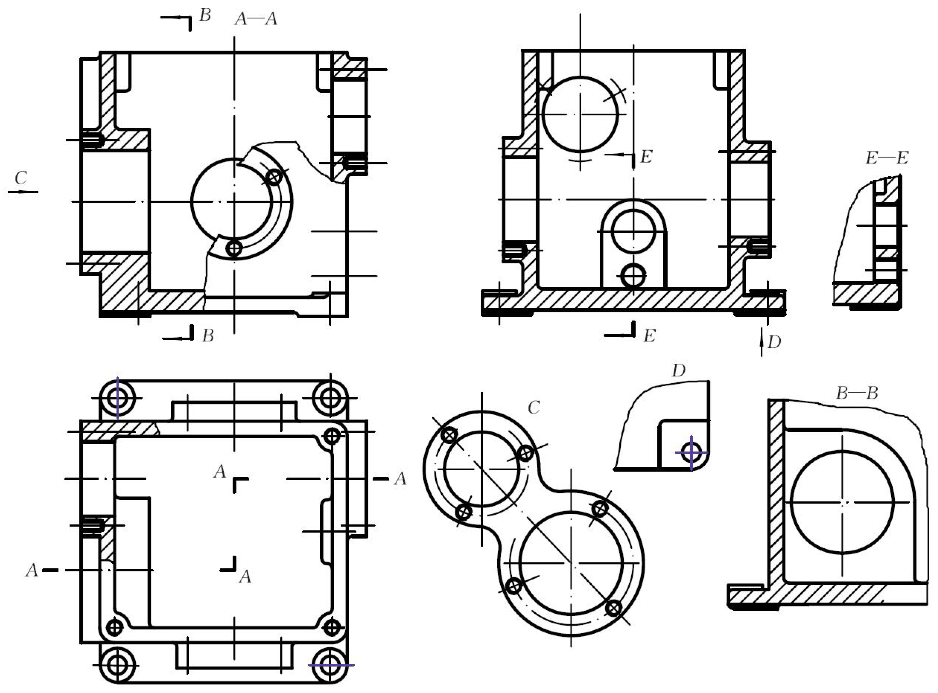
Figure 4.
After two transformations, point A is moved onto the projection axis.
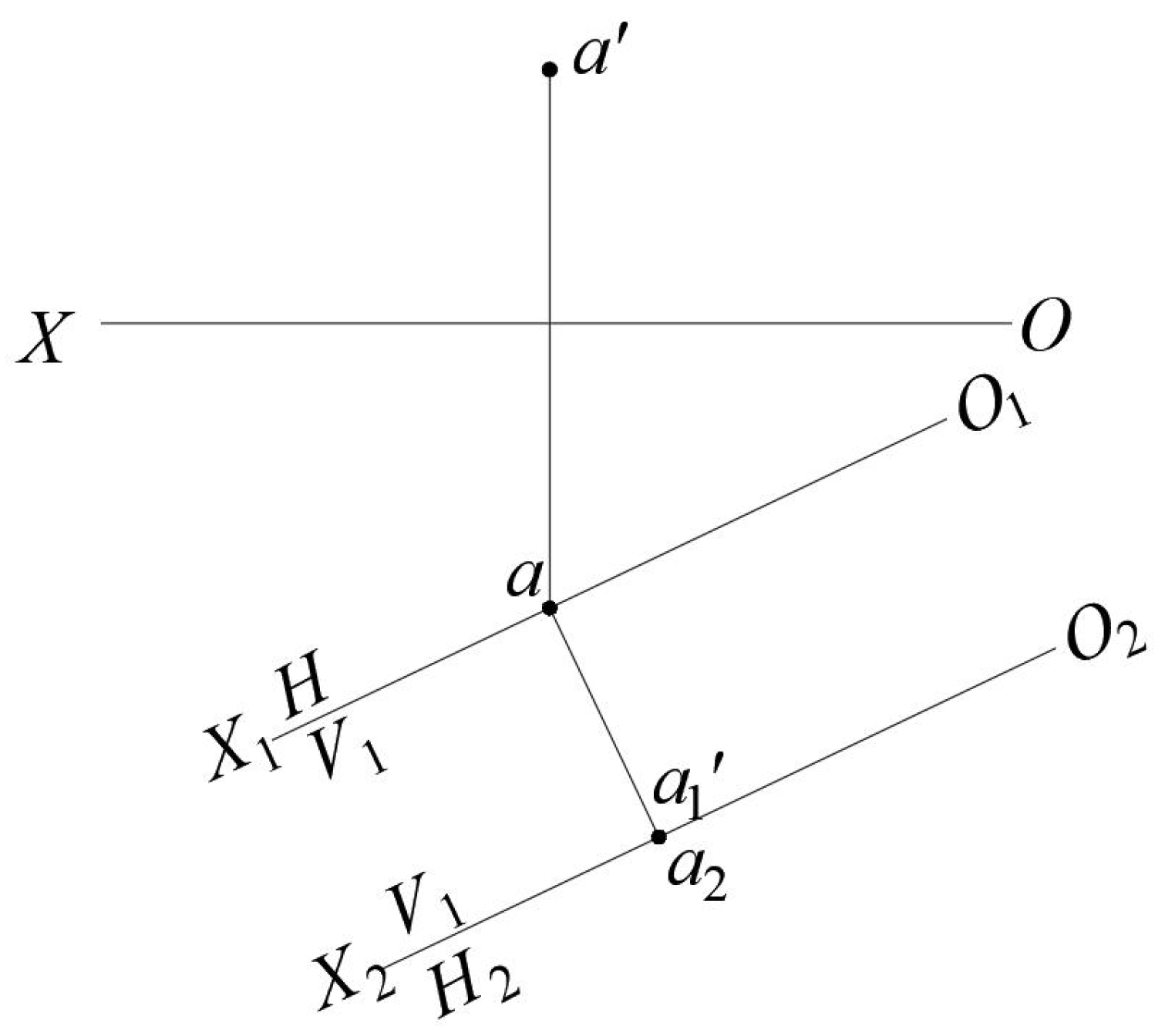
Figure 5.
Transform the general position line MN into a line perpendicular to the projection plane through two successive changes of planes.
Figure 5.
Transform the general position line MN into a line perpendicular to the projection plane through two successive changes of planes.
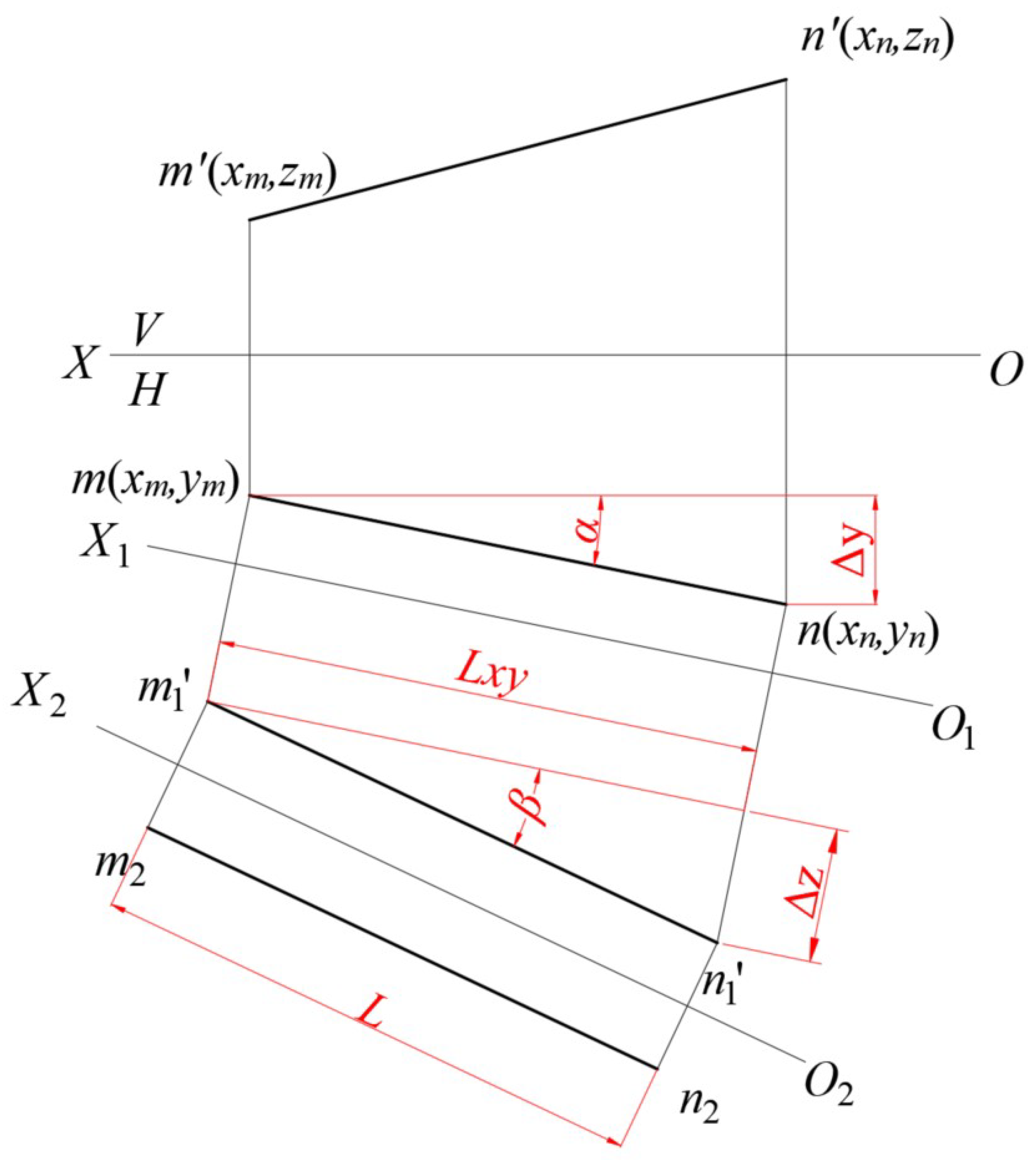
Figure 6.
The vector representation method of a spatial line segment.
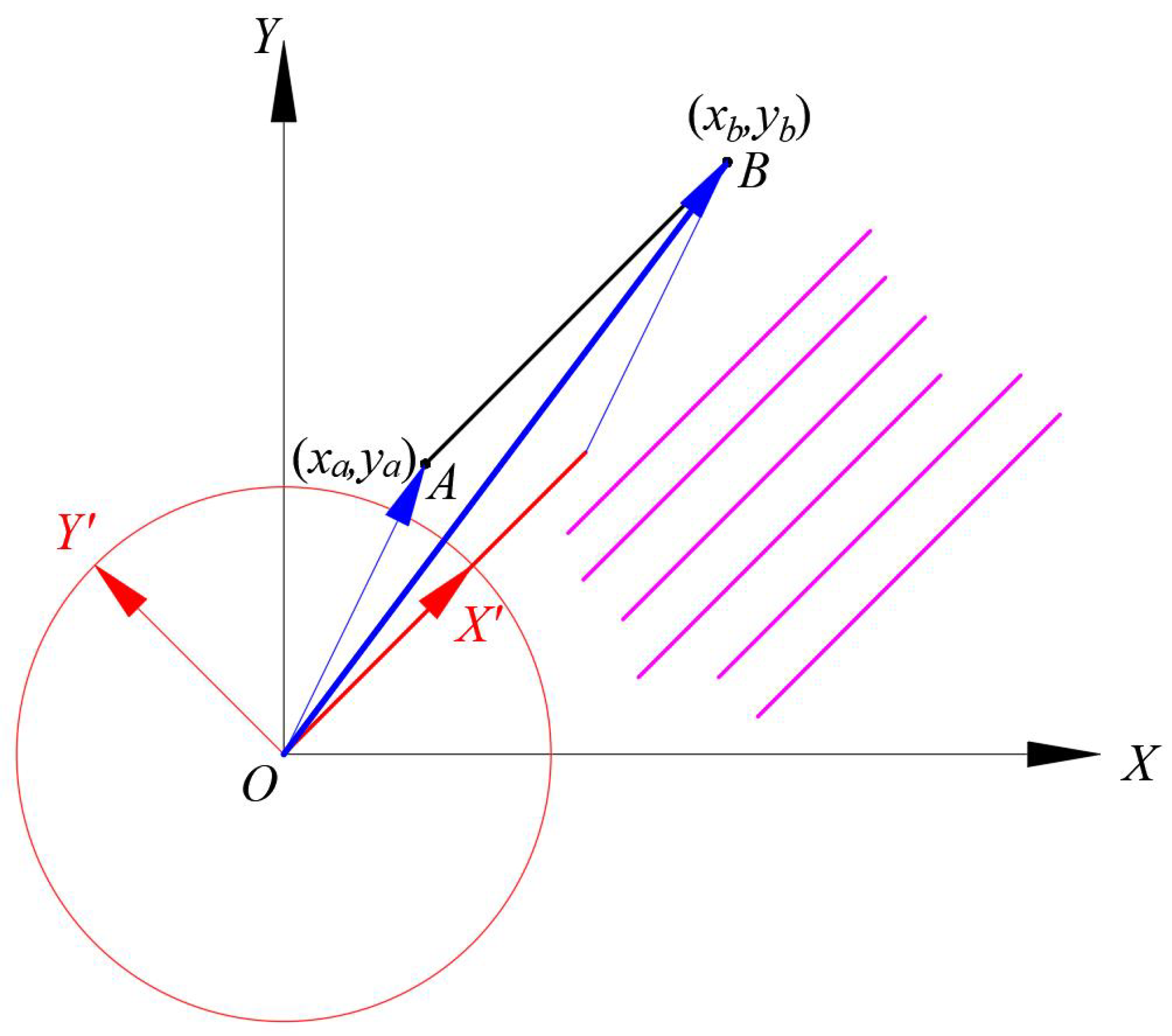
Figure 7.
A planar polygon in three-dimensional space.
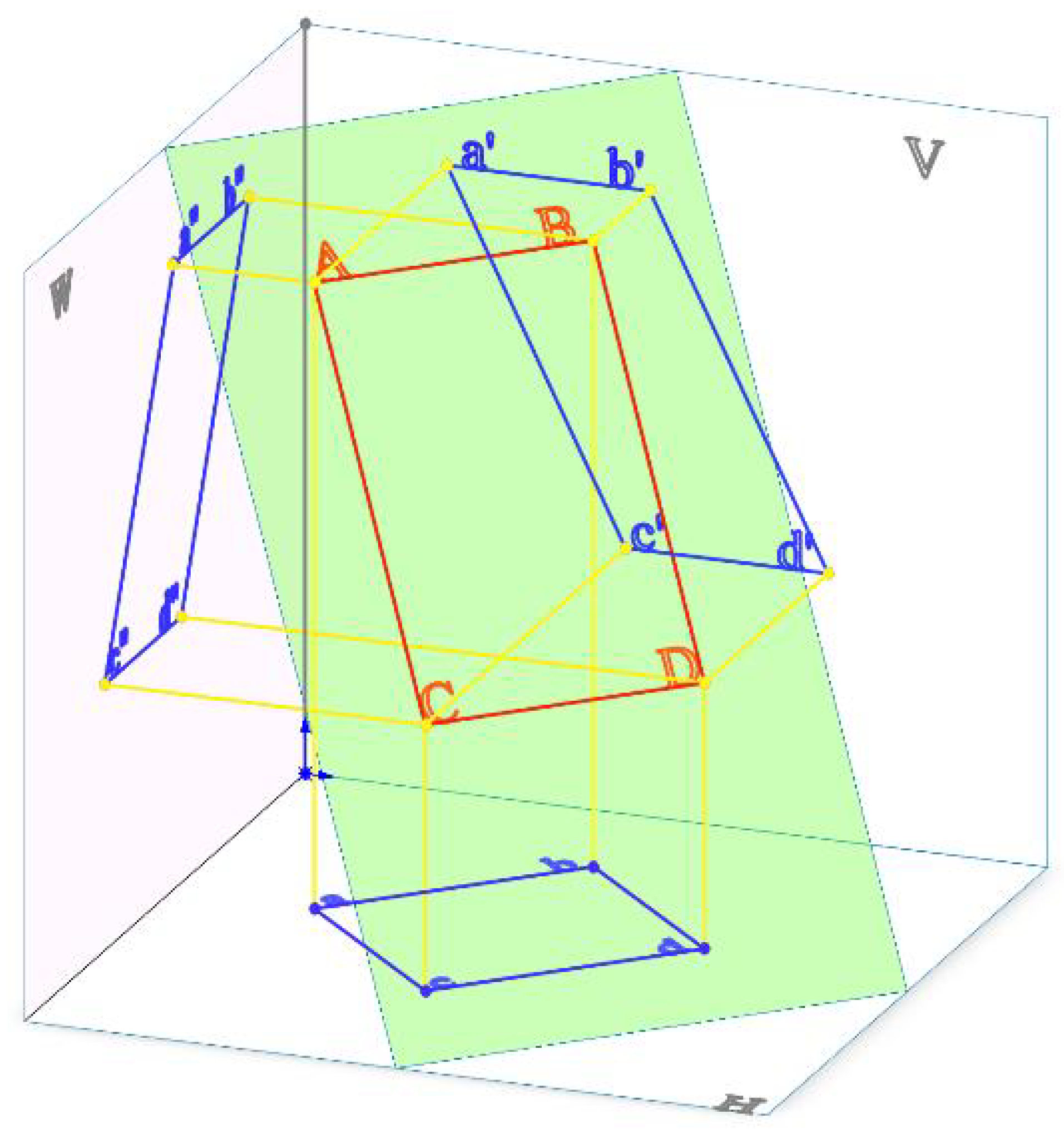
Figure 8.
Sparse representation of planar shapes.
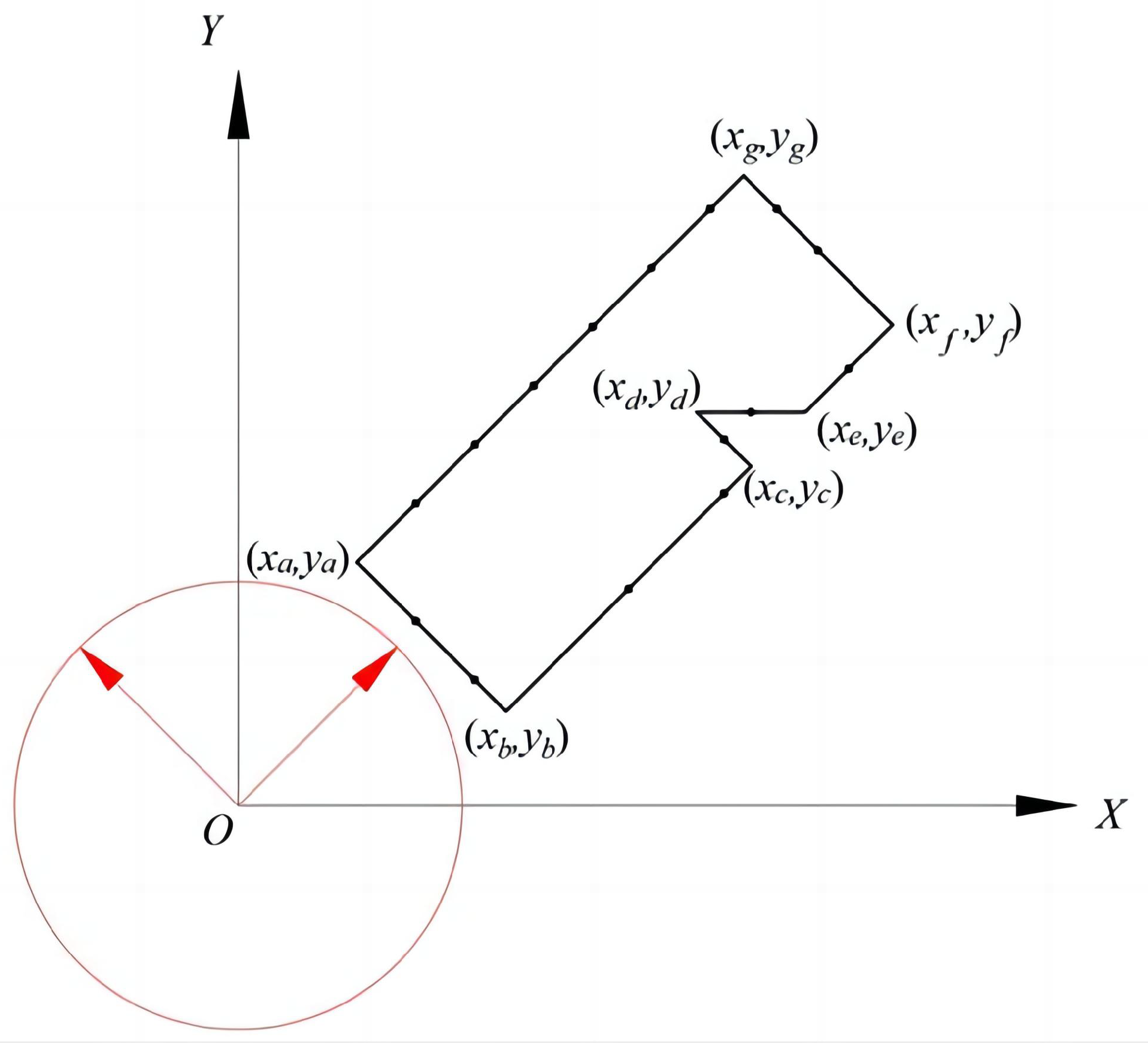
Figure 9.
Cubes in general position.
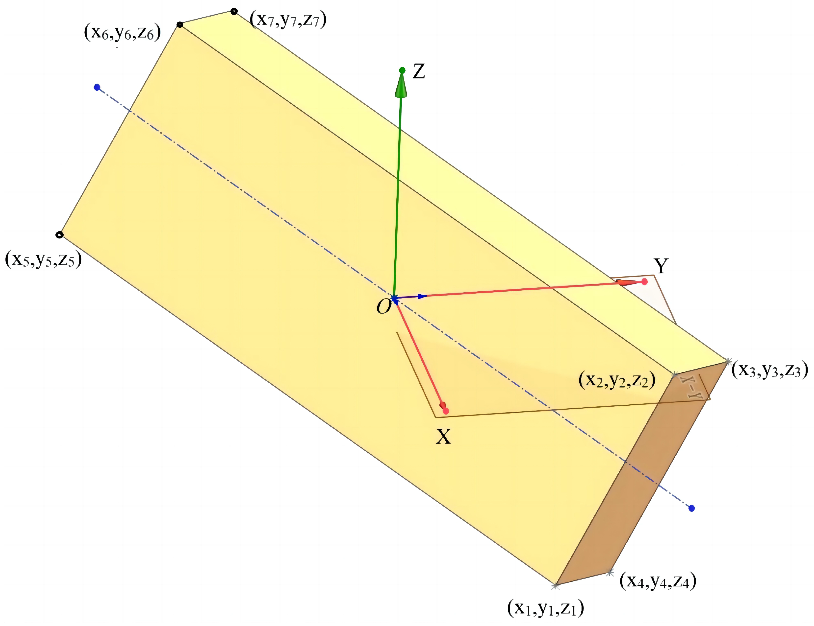
Figure 10.
Use the principle of axonometric axis selection to obtain a new projection plane system by the method of change plane.
Figure 10.
Use the principle of axonometric axis selection to obtain a new projection plane system by the method of change plane.
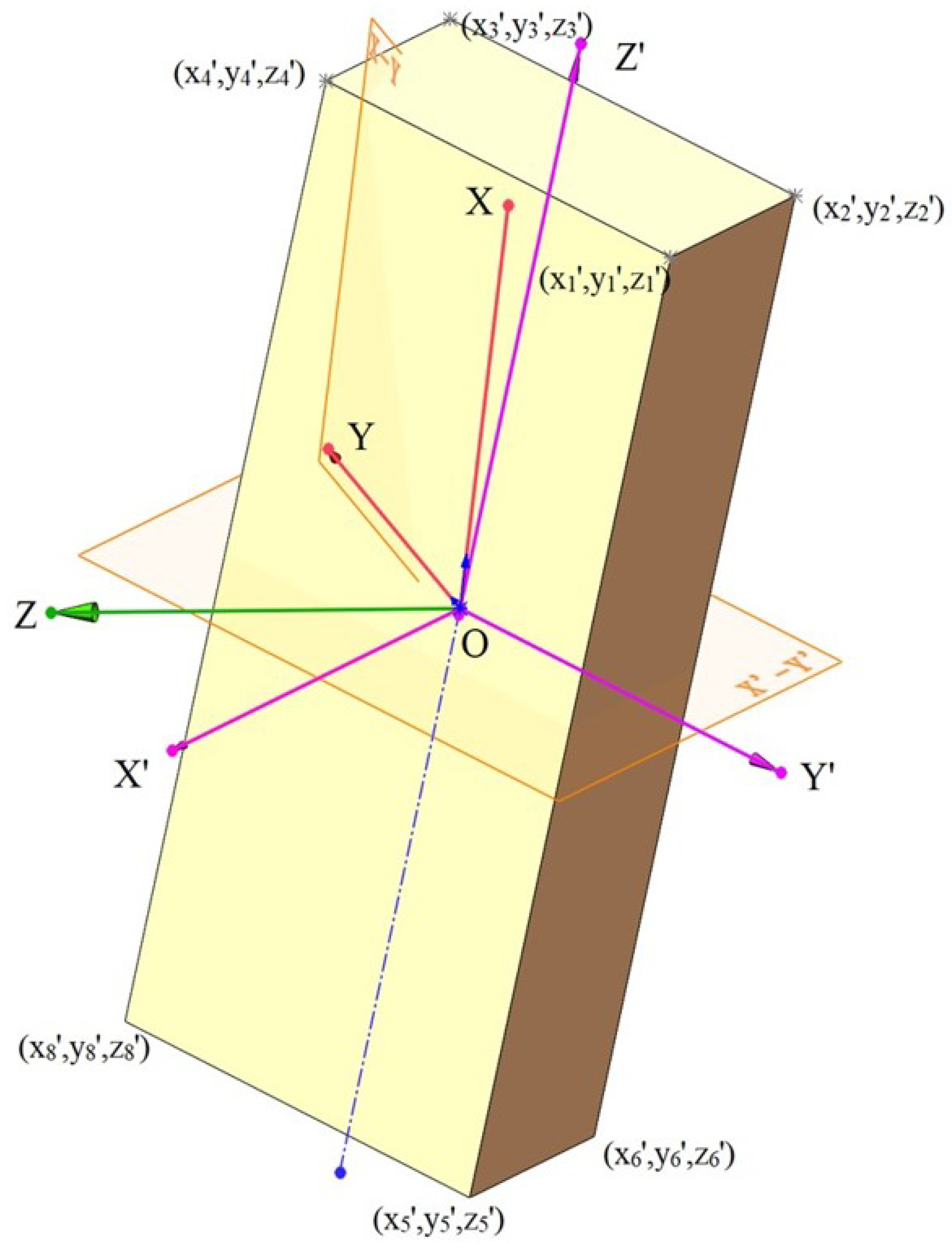
Figure 11.
Changing-plane method.
Disclaimer/Publisher’s Note: The statements, opinions and data contained in all publications are solely those of the individual author(s) and contributor(s) and not of MDPI and/or the editor(s). MDPI and/or the editor(s) disclaim responsibility for any injury to people or property resulting from any ideas, methods, instructions or products referred to in the content. |
© 2025 by the authors. Licensee MDPI, Basel, Switzerland. This article is an open access article distributed under the terms and conditions of the Creative Commons Attribution (CC BY) license (http://creativecommons.org/licenses/by/4.0/).
Copyright: This open access article is published under a Creative Commons CC BY 4.0 license, which permit the free download, distribution, and reuse, provided that the author and preprint are cited in any reuse.


