
Submitted:
05 April 2025
Posted:
08 April 2025
You are already at the latest version
Abstract
In this paper, we study the 2D Shape Equipartition Problem (2D-SEP) with minimal boundaries and we propose an efficient method that solves the problem with low computational cost. The goal of 2D-SEP is to obtain a segmentation into N equal area segments (regions), where the number of segments (N) is given by the user, under the constraint that the length of boundaries between the segments is minimized. We define the 2D-SEP and we study problem solutions using basic geometric shapes. We propose a 2D Shape Equipartition algorithm based on a fast balanced clustering method (SEP-FBC) that efficiently solve the 2D-SEP problem under complex 2D shapes in O(N·|S|·log(|S|)), where |S| denote the number of image pixels. The proposed SEP-FBC method initializes clustering using centroids provided by the k-means algorithm, which is executed first. During each iteration of the main SEP-FBC process, a region-growing procedure is applied, starting from the smallest region and expanding until regions of equal area are achieved. Additionally, a Particle Swarm Optimization (PSO) method that uses the SEP-FBC method under different initial centroids, has been also proposed to explore better 2D-SEP solutions and to show how the selection of the initial centroids affect the performance of the proposed method. Finally, we present experimental results on more than 2,800 2D shapes to evaluate the performance of the proposed methods and illustrate that their solutions outperform other methods from the literature.
Keywords:
shape analysis
; image segmentation
; equipartition
; geometric shapes
1. Introduction
Image segmentation is a fundamental problem in the fields of computer vision and pattern recognition and plays a crucial role in a wide range of applications. These applications span various domains, including object recognition [1], remote sensing [2,3], and medical image analysis [4,5]. At its core, image segmentation involves the division of an image into meaningful regions or segments, facilitating higher-level analysis and interpretation. The task can be formulated in two principal ways: as a classification problem at the pixel level, known as semantic segmentation, or as an object-specific partitioning problem, referred to as instance segmentation.
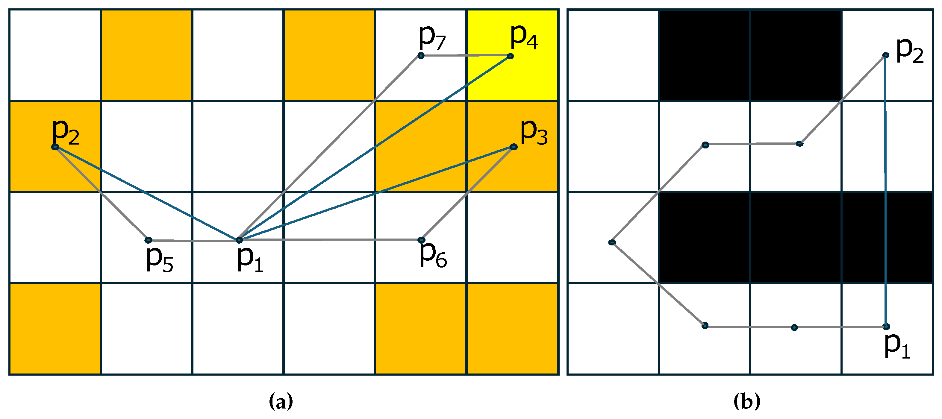
The curve equipartition problem has been formally defined, explored, and solved in [6]. This problem has numerous applications across various domains, including polygonal approximation [7], signal modeling [8], video summarization [9]. The objective of the curve equipartition problem is to identify consecutive points along a given curve such that the curve is divided into N segments of equal chord lengths under a predefined distance function (see Figure 1 and Figure 2). This partitioning ensures that each segment maintains a consistent measure in terms of the chord length, which makes it highly relevant in geometric and computational applications. In [6], a level set approach is adopted to establish that for any continuous injective curve in a metric space and for any given number N, there always exists at least one valid N-equipartition. Furthermore, an approximate algorithm inspired by the level set approach is proposed to efficiently compute all possible solutions with high accuracy. The number of solutions to this problem generally depends on both the shape of the curve and the chosen value of N. In particular, for certain special classes of curves, the number of solutions for some values of N may be infinite. A geometric proof, provided in [6], demonstrates that the curve equipartition problem always has at least one solution for every continuous injective curve, regardless of the number of partitions.
Figure 2 illustrates the three distinct solutions for the curve equipartition problem with . In this figure, the computed partition points (depicted in green) are projected onto the curve (represented by the blue curve) and are connected by red line segments. An interesting extension of the curve equipartition problem involves generalizing its formulation and solution techniques to different mathematical and computational structures, including meshes [10], images [4], and shapes [11,12]. These extensions open up new avenues for research and practical applications in geometric processing, computer vision, and pattern recognition.
In our previous work [12], a general version of the 2D shape equipartition problem (2D-SEP) with minimum intrinsic boundary length has been presented. According to the 2D shape equipartition problem, the goal is to compute a shape segmentation into N equal area segments, so that the length (L) of the intrinsic boundary between the segments is minimized. We have shown that for any convex shape S, the 2D-SEP problem has at least one solution for any value of N, even if the intrinsic boundaries are line segments. However, when a non-convex 2D shape is given, there exist some cases where the 2D-SEP has no solution even for . In [12], two methods have been proposed to solve 2D-SEP:
- a region growing based method that solves the general version of 2D-SEP problem called SEP-RG, and
- a sequential selection method that efficiently solves the problem under the constraint that the intrinsic boundaries are line segments called SEP-ILS.
In this work, we study in more depth the 2D shape equipartition problem (2D-SEP) studying optimal solutions for basic geometric shapes. Additionally, we propose two methods for solving 2D-SEP:
- a 2D Shape Equipartition algorithm based on a fast balanced clustering method (SEP-FBC), and
- a Particle Swarm Optimization (PSO) method that uses the SEP-FBC method, called SEP-PSO FBC.
SEP-FBC uses initial seeds as SEP-RG, but instead of successive executions of region growing steps of SEP-RG, firstly it performs hard clustering and then performs a growing—shrinking process that gradually improves satisfaction with the criterion of equal area regions. This results in a low computation cost method that makes possible its integration with Particle Swarm Optimization (PSO) framework, resulting on the top performing method SEP-PSO FBC. To our knowledge, SEP-FBC is the most computationally efficient method to solve 2D-SEP. According to our experimental in more than 2,800 2D shapes, the proposed methods clearly outperform in terms of intrinsic boundary length the current methods from literature (SEP-RG and SEP-ILS).
Figure 3 presents examples of the proposed 2D-SEP for different numbers of segments (). In the first and second rows the results come from the SEP-ILS and SEP-RG methods [12], respectively. In the third row, the corresponding results come from the proposed SEP-FBC method. In any case, the segmentation consists of N equal-area segments. However, the intrinsic boundary length (L) differs by method. Figure 3a shows a segmentation of an apple for , where a solution of a line segment close to the diameter of the apple seems to be the optimal solution of 2D-SEP. In this simple example, as expected, the SEP-ILS method, which exclusively uses line segments, yields the lowest intrinsic boundary length . Figure 3i shows a corresponding segmentation using the proposed SEP-FBC method that yields a slightly higher intrinsic boundary length . In more complex examples (see Figure 3i–l), the proposed SEP-FBC method yields a lower intrinsic boundary length than the other methods.
In summary, the main contributions of our work are the following:
- To the best of our knowledge, this is the first work that extensively studies the 2D-SEP problem under minimum intrinsic boundary length.
- We propose a fast balanced clustering method (SEP-FBC) that can be combined with Particle Swarm Optimization (PSO) framework due to its low computational cost to efficiently solve the general version of the 2D-SEP problem.
- The quantitative results obtained on more than 2,800 2D shapes included in two standard datasets quantify the outer performance of the proposed methods from baselines of the literature.
The rest of this paper is organized as follows: Section 2 reviews the related work for image segmentation and balanced clustering methods. The 2D-SEP problem formulation is given in Section 3. 2D-SEP instances and properties are studied in Section 4. Section 5 presents the two proposed methods for solving 2D-SEP, respectively. Section 6 describes the experimental setup along with the results obtained. Finally, conclusions and future work are provided in Section 7.
2. Related Work
The problem of image segmentation segmentation has been studied extensively during the last decades. In the literature, a variety of image segmentation techniques have been proposed, each utilizing different principles and methodologies. Traditional approaches include thresholding methods [13], region-growing techniques [14], and region-merging strategies [15]. Other widely used techniques involve clustering methods, such as k-means [16], and edge-based methods such as watershed segmentation [17]. Furthermore, contour-based techniques, such as active contours [18], and graph-based methods, including graph cuts [19], have demonstrated effectiveness in various applications. Probabilistic approaches, such as conditional and Markov random fields [20], as well as sparsity-based methods [21], have been explored for robust segmentation under challenging conditions.
In recent years, the advent of deep learning (DL) has revolutionized the field of image segmentation, leading to significant improvements in accuracy and generalization. Deep learning models leverage hierarchical feature extraction and end-to-end learning capabilities to surpass traditional methods in performance. Convolutional neural networks (CNNs) and their advanced architectures, including fully convolutional networks (FCNs), U-Net, DeepLab, and Mask R-CNN, have established new benchmarks in image segmentation tasks in multiple domains [22]. These advances have enabled the development of highly accurate automated segmentation systems, facilitating progress in medical diagnostics, autonomous driving, and many other critical applications.
Different error criteria have been proposed for image segmentation problems. The Intersection Over Union (IoU) and the F-measure are two of the most popular supervised methods to evaluate image segmentation quality, but it requires the ground truth [23]. Under unsupervised image (color or grayscale) segmentation methods, where the ground truth is completely unknown, clustering based criteria such as the heterogeneity of pixels between regions and the homogeneity within the region objectively can be used to evaluate the segmentation [24].
Under 2D-SEP problem, no ground truth is given. So, we have to select an unsupervised criterion. Additionally, the given image is binary, so no color-grayscale imformation is given. Similarly with the polygonal approximation [25] problem, the 2D-SEP problem can be formulated in two ways:
- The problem of minimum error, where the error (e.g., boundary length) is minimized given the number of segments N.
- The problem of minimum number of segments, where the approximation error is bounded and the goal is to find the minimum number of segments (N) that gives error lower than the given error.
In this work, according to the proposed problem formulation, we select the first problem formulation of error minimization given the number of segments N, under the error criterion of minimum intrinsic boundary length that may better divide the shape into N equal area segments. The intrinsic boundary length criterion is selected since in the given shape S there does not exist color information, model error, or weights for the boundaries to use a more complicated criterion. Additionally, the same idea called minimum cut has also been used in image segmentation [26].
Apart from image segmentation, the 2D-SEP problem is related to the balanced clustering problem in the sense that the goal of 2D-SEP is to group the pixels into balanced in-area regions. Clustering is an important problem in a broad spectrum of applications, such as data mining, computer vision, machine learning and pattern recognition [27]. Thousands of clustering algorithms have been proposed in the literature in many different scientific disciplines [28] that differ in the choice of the objective function, probabilistic generative models, and heuristics. Clustering algorithms can be divided into two main categories: hierarchical and partitional [28]:
- Hierarchical clustering algorithms recursively find nested clusters in either an agglomerative (bottom-up) mode or in a divisive (top-down) mode.
- According to partitional clustering algorithms, the clusters are simultaneously computed as a partition of the data. Usually, the partition is based on a local optimization of a given criterion.
K-means clustering algorithm [29], is one of the simplest partitional clustering algorithms that solves the clustering problem for a given number of clusters. Even though K-means was first proposed over 50 years ago, it is still one of the most widely used algorithms for clustering. K-means is a centralized clustering algorithm with linear computation cost. The goal of K-means is to minimize the sum of squared error (SSE) over all clusters which is an NP-hard problem even for . K-means starts with K centroids, e.g., randomly selected in d-dimensional space, one for each candidate cluster. K-means converge to a local minimum of SSE. So, in the case where the given datasets consist of spherical and/or well-separated clusters, these centroids will eventually be placed at the centers of the clusters. In [30], a variant method (K-means++ algorithm) for centroid initialization has been proposed that chooses centers at random from the data points but weighs the data points according to their squared distance from the closest center already chosen. K-means++ usually outperforms K-means in terms of both accuracy and speed. An extension/variation of K-means is the K-medoid or Partitioning Around Medoids (PAM) [31], where the clusters are represented using the medoid of the data instead of the mean. Medoid is the object of the cluster with minimum distance to all other objects in the cluster.
Traditional clustering aims to minimize the mean square error without considering the balance of the cluster size. Balanced clustering is a 2-objective optimization problem, in which two objectives contradict each other: to minimize error and to balance cluster sizes [32]. In hard balance-constrained clustering, cluster size balance is a mandatory requirement that must be met, and minimizing Mean Square Error is a secondary criterion. Balance-constrained clustering can be solved in O(), using a balanced k-means clustering algorithm that solves the assignment problem by Hungarian algorithm [32], where S denotes the number of points. In soft-balanced clustering, balance is an aim but not a mandatory requirement. In [33], a soft balanced clustering method based on k-means clustering algorithm and network simplex methods has been proposed.
3. Problem Formulation
The 2D Shape Equipartition Problem (2D-SEP) under minimum intrinsic boundary length [12] is formulated hereafter. Let S be a given shape and N be the given the number of equal area segments (regions). Let be a segmentation of S. Each region , should be connected, which means that the pixels in the segment belong to the same connected component. Let be the common boundary between the regions and , . Then, the optimal segmentation of 2D-SEP should satisfy the following constraints:
where denote the cardinality operation, e.g., gives the area of shape S (number of pixels).
where the total intrinsic boundaries’ length of segmentation R:
where denotes the length of boundary . In image processing with pixel accuracy the satisfaction of Equation (1) is impossible in the case that the area of shape S is not exactly divided by N and at the same time the equality constraint is very hard. Therefore, in this work we have relaxed Equation (1) as follows:
where is set equal to , resulting in a mandatory but realistic (feasible) requirement that should be satisfied.
Furthermore, in our experimental results we allow comparisons between different shape sizes and scales by using the normalized total intrinsic boundary length () of the segmentation R, defined as the ratio of to the outer boundary length of the object .
4. 2D-SEP Instances and Properties
In the following, we study basic instances and properties of 2D-SEP.
4.1. Plane Partition
Firstly, we will consider the case of partitioning of a plane into a high number of equal area regions. Figure 4 shows three popular regular tessellation patterns (equal area regions) that can tile a plane without overlaps or gaps: tessellations using (equal) hexagons, squares, or equilateral triangle. According to 2D-SEP, we examine the efficiency of the above three patterns in Table 1 by comparing the boundaries of an equal area (s) hexagon, square and equilateral triangles as a function of s. We find that tessellations using hexagons have and lower intrinsic boundary lengths compared to tessellations using square and equilateral triangles, respectively. Theoretically, SEP-FBC and SEP-RG is possible to generate hexagonal and square tessellations, while SEP-ILS is possible to generate only equilateral triangle tessellations. Consequently, SEP-FBC and SEP-RG hold a theoretical advantage over SEP-ILS, a finding that is further supported by our experimental results.
Hales [34] gives proof that any partition of the plane into regions of equal area has a perimeter at least that of the regular hexagonal honeycomb tiling, meaning that the optimal solution of 2D-SEP when the number of regions is large enough is the partition into equal hexagonals.
4.2. 2D-SEP of Square and Circle
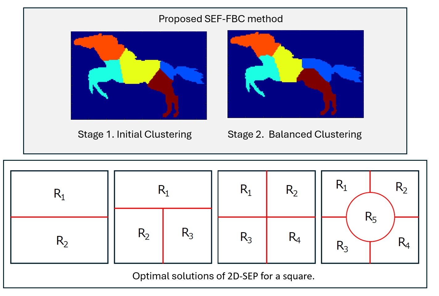
Next, we consider the case of partitioning of a square and circle into two, three, four and five equal area regions. To provide comparable numerical results, we assume a unit area square and circle. Figure 5 depicts optimal solutions of the 2D-SEP for unit area ((a)-(d)) square and ((e)-(h)) circle under N = 2, 3, 4 and 5. While, Figure 5 shows some suboptimal solutions of the 2D-SEP for unit area ((a),(b)) square and ((c),(d)) circle for . Taking into account both figures, the optimality proof of most cases in Figure 5 is trivial, so hereafter we only provide the close form of the intrinsic boundary length (L), which is numerically reported in the caption of the figure.
- When N = 2 (see Figure 5 a,e), the optimal solution of 2D-SEP under square and circle is given the horizontal line that passes from the square centroid () and the diameter of the circle (), respectively.
- When N = 3 (see Figure 5 b,f), the optimal solution of 2D-SEP under square is given by two suitable vertical lines that divide the square into three rectangles , , with . The optimal solution of 2D-SEP under circle is given boundary of the three radius that passes from the center with .
- When N = 4 (see Figure 5 c,g), the optimal solution of 2D-SEP under square is given by two suitable vertical lines that cross at the square centroid and divide the square into four equal squares, with . The optimal solution of 2D-SEP under circle is given similarly by two vertical diameters with .
- When N = 5 (see Figure 5 d,h), the optimal solution of 2D-SEP under square is given by a circle of radius ( plus four suitable vertical lines of length (), with . The optimal solution of 2D-SEP under circle is given by five radius with that is slightly lower than the corresponding solution of Figure 6d with .
An interesting remark of the above examples is that in any case the L of the optimal solution of the square is lower than the corresponding L of the circle. The proof that this is true (or this is not true) for any value of N is an open problem.
In Figure 7, we provide the corresponding results of the proposed method SEP-FBC under unit area square and circle and to compare with the optimal 2D-SEP solutions of Figure 5. We find that in any case of circle SEP-FBC results the optimal solution, while in two out of five cases of square (, ), the proposed segmentation of SEP-FBC is suboptimal with slightly higher L than the optimal one:
4.3. Intrinsic Boundaries’ Length
Hereafter, we study an important 2D-SEP property, the sequence of the total intrinsic boundaries’ length of the optimal 2D-SEP solution of shape S into N regions, as N increases. According to the problem definition, it holds that
since the area of its region, as N tends to ∞, it tends to zero, so the total intrinsic boundaries’ length tends to ∞, covering the whole space of the shape S. When , the depends on shape S. The following inequality provides the upper bound of the
where denotes the perimeter of shape S. The proof is trivial for convex shapes by getting the suboptimal solution that the intrinsic boundaries are line segments . This solution always exists for convex shapes [12] and it satisfies the Inequality (7).
The fact that may be a monotonically increasing sequence for some shapes is also supported by the Inequalities (6) and (7), and it is true for several simple shapes and at least for low values of N.
However, there exist some shapes in which even for low values of N (e.g., ), the Inequality (8) is not true. Figure 8 depicts a shape that consists of three successive circles of radius, where
The red and gray lines show the intrinsic boundary for the optimal segmentation into two and three regions, respectively. Since in this constructed example can be set almost zero, it holds that
Similarly, with the case of three circles, in the corresponding shape with successive circles , it holds that
In Section 6.5, we study the sequence of the solutions derived by the proposed methods. Since, the sequence may be monotonically increasing for low values of N and simple shapes, it can measure the complexity of the dataset. Furthermore, if we compare the derived sequence for different methods, conclusions can be drawn about the robustness of the methods, as is expected to increase.
5. Methodology
5.1. SEP-Fast Balanced Clustering
This Section presents the proposed Fast Balanced Clustering method (SEP-FBC) that sub-optimally solves the 2D-SEP in O(), where denote the number of image pixels. The pseudo-code of the proposed SEP-FBC method is given in Algorithm 1. The input of SEP-FBC is the shape S (e.g., a binary image) and the number of the desired regions N of equipartition. The output is the segmentation R according to the constraints of the problem, as defined in Section 3. In the following, we analyze all the steps of the SEP-FBC method. SEP-FBC consists of two stages:
In the first stage, hard clustering of shape pixels is performed (lines 1-16 of Algorithm 1).
- Initially, a graph G of the connected pixels from the 2D image space of shape S is computed using eight pixel connectivity. This graph is used to approximate the shortest path distance between the shape points of the complete graph (see Appendix A).
- Then, an initial estimation of the centroids of the N clusters () is calculated by the k-means++ method [30] (with computational cost ) followed by the round operation to adjust C to the space of the image coordinates (see line 1 of Algorithm 1). In the case where does not belong in shape S (), is set to the nearest shape pixel (see lines 4-6 of Algorithm 1). The centroid corresponds to the region .
- Furthermore, we initialize each region and compute for each region the vector with the all the 8-connectivity graph based distances between the centroid and the shape points (see lines 7-8 Algorithm 1)1. The initial clustering of shape pixels is performed using an approximation by the combination of the Euclidean distance and (see line 12 of Algorithm 1) of the graph-based distance of a complete graph of shape S. The use of graph-based distances for clustering provides better image component connectivity for clusters compared with the use of the pure Euclidean distance. The sum of boundaries’ lengths of the resulting segmentation is low due to the distance-based clustering procedure, but the clusters’ sizes may not be equal.
In the second stage, the resulting clustering is balanced (lines 17-23 of Algorithm 1).
- Initially, we ensure that all the clusters (regions) consist of connected pixels by assigning non-connected pixels to the smallest neighbor region (see line 17 of Algorithm 1). Additionally, we smooth the region boundaries by reassigning the pixels of each region boundaries to the region that has the most neighbors.
- Finally, we perform an iterative process that in each iteration grows the smallest region (areaGrow procedure) until the Inequality (4) is satisfied (see lines 20-23 of Algorithm 1). The symmetric matrix that counts the number of pixel reassignments between two regions is initialized to zero. The areaGrow procedure uniformly grows the smallest region c by applying the dilation operation with an open disk of radius one. The procedure prevents infinite loops by adding the extra pixels p in a descent way according to expression , where denotes the area of the region to which p belonged, is the number of reassignments between the regions c and the region that p belonged (). The procedure can stop before growth has finished, only if the current area of the region is at least . The computational cost of this stage is according to the procedures of lines 17-19 of Algorithm 1. The iterative step of lines 20-23 of Algorithm 1 has a computational cost of .
Taking into account all the steps of the method, we get a total computation cost equal to that is simplified to , since .
| Algorithm 1: The proposed SEP-FBC method. |
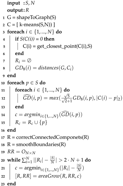 |
Figure 9 shows some segmentation results of the two stages of the proposed SEP-FBC method for . Figure 9a shows the result of the first stage of the method with a total intrinsic boundary length equal to , which produces regions of varying areas in the range . The execution of the second stage (see Figure 9b) yields equal area segments with a total intrinsic boundary length equal to . In another example of Figure 9c the result of the first stage has the total intrinsic boundary length with regions of varying areas in the range . The execution of the second stage (see Figure 9d) results in equal area segments with a total intrinsic boundary length .
5.2. SEP-PSO Fast Balanced Clustering
This Section presents the proposed Particle Swarm Optimization (PSO) based Fast Balanced Clustering method (SEP-PSO FBC), which combines the PSO framework with the proposed SEP-FBC method to improve its results.
PSO is a derivative-free optimization method designed to handle complex, multi-modal, and discontinuous objective functions with multiple local minima. The optimization process is driven by the evolution of a population (swarm) of candidate solutions (particles). These particles explore the parameter space of the objective function, adapting over a finite number of generations (iterations) based on a strategy that emulates “social interaction.” The key parameters of PSO are the number of particles and generations, whose product defines the computational budget—that is, the total number of objective function evaluations. PSO is capable of achieving near-optimal solutions and has been successfully applied to various challenging optimization problems in computer vision and pattern recognition, including classification, clustering, prediction, simplification, image segmentation, video co-segmentation, and object tracking [25,35,36,37,38,39].
According to the 2D-SEP problem definition, the proposed SEP-PSO FBC method optimizes the metric (see Equation (3)) for initial centroids, which initialize SEP-FBC method (instead of k-means initialization), that are directly represented by PSO particles. Similarly with SEP-FBC, the input of SEP-PSO FBC is the shape S and the number of the desired regions N of equipartition, and the output is the segmentation R according to the constraints of the problem, as defined in Section 3.
Iteratively, PSO searches for the best combination of N initial centroids that minimize the metric. We represent each particle by a vector with the 2D coordinates of the N-initial centroids of the regions. In order to reduce the search space, we assume that the vertices are sorted in ascending order concerning their distance from the top-left image corner; otherwise, in the evolution process, we correct the order of vertices of each particle according to this hypothesis. The fitness (objective function) of the particle is directly given by the metric of the particle (see Equation (3)). The SEP-PSO FBC algorithm is analytically described hereafter.
Initially, we create a population of M particles (e.g., ) that are located in random positions in shape S, while the first particle is given by the k-means++ algorithm (see Section 5.1). In the evolution process, PSO finds the current optimal solution in order to update the best global solution. Furthermore, the best local solution for each particle is also updated, where the of the particle reaches a better solution. The method ends when the number of iterations of the evolution process exceeds the given number of generations. In this work, we use the upper limit of 50 generations.
6. Experimental Evaluation
6.1. Datasets
The proposed approaches were evaluated using two well-established datasets from the literature. More specifically, we employ:
Figure 10 shows twelve sample images from the LEMS dataset and the MPEG-7 dataset.
6.2. Baseline Methods
We compared the performance of the proposed methods (SEP-PSO FBC, SEP-FBC) with the baselines SEP-RG and SEP-ILS algorithms [12] that also solve 2D-SEP. Both baselines are briefly presented in Section 1. The methods are evaluated for a sufficient number of consecutive values of N, starting from , the minimum value at which 2D-SEP can be defined. Therefore, in our experiments, we have evaluated the methods for nine different values of . Additionally, the SEP-PSO FBC framework is compared with the SEP-FBC to show how the selection of the initial centroids affects the performance of the method SEP-FBC.
All the analysis has been done using MATLAB 2023b on an Intel i7 core 3.20GHz with 32 GB RAM without the use of code optimization or parallel processing tools. The code implementing the proposed methods along with the data sets will be publicly available online after acceptance of the paper: https://sites.google.com/site/costaspanagiotakis/research/shape-equipartition.
6.3. Evaluation Metrics
Based on the formulation of the 2D-SEP problem, we have compared the performance of SEP-PSO FBC, SEP-FBC, SEP-RG and SEP-ILS on the normalized total intrinsic boundary length (see Section 3). For a given dataset, we also compute , where m is a method in . is defined as the percentage of shapes of the datasets where the method m outperforms the others under the , defined as follows:
where, H is the unit step function, denotes the number of shapes of dataset D and is the metric of method m given the shape S. This also means that the value gives the percentage of images for which there is no clear winner method. In addition, we study the computational efficiency of all methods by measuring the Average Execution Time () per image for different values of N.
Furthermore, in this work, we use the circularity () and solidity () shape descriptors [43] to show that the used datasets consist of quite different shapes and to measure how the performance of the proposed methods is affected by the complexity of the shapes. Circularity () is defined by the ratio of the area of the shape multiplied by the product divided by the square of the perimeter of the shape (). The circularity of a circle is one (maximum value) and the lower it goes, the less circular it is or having a more complex outer boundary.
Solidity () is defined by the proportion of pixels in the convex hull that are also in the region. Solidity describes the extent to which a shape is convex or concave. The solidity of a completely convex shape is one; the farther the solidity, the greater the extent of concavity in the structure. Figure 11a shows the circularity and solidity relative frequency histogram for the LEMS and MPEG-7 datasets, highlighting the diversity of shapes found in both datasets.
6.4. Comparisons on LEMS and MPEG7 Datasets
In the following, we present comparisons of the proposed and baseline methods on the normalized total intrinsic boundary length () and in terms of computational efficiency. Figure 12 shows the average for nine different values of of SEP-PSO FBC, SEP-FBC, SEP-RG and SEP-ILS methods computed on MPEG7 and LEMS datasets. We find that SEP-PSO FBC clearly outperforms the other methods in any dataset under and metrics. It should be noted that UPF-FBC is clearly the most computationally efficient method, since it is about six, thirty and sixty times faster than SEP-RG, SEP-PSO FBC and SEP-ILS, respectively. SEP-FBC also outperforms SEP-RG and SEP-ILS under intrinsic boundary length. SEP-RG outperforms SEP-ILS under intrinsic boundary length and computational cost.
Figure 12 shows NL metric of the SEP-PSO FBC, SEP-FBC, SEP-RG and SEP-ILS methods computed on LEMS and MPEG7 datasets for different values of N. We find that for any data set and value of N, SEP-PSO FBC clearly outperforms the other methods. More specifically, SEP-PSO FBC produces a lower NL than SEP-PSO ranging from on the LEMS and MPEG7 datasets. SEP-PSO FBC produces a lower NL than SEP-RG ranging from on the LEMS and MPEG7 datasets. SEP-ILS outperforms SEP-RG and SEP-ILS under any dataset and value of N. Therefore, the results of the figure agree with the corresponding results of Table 2, showing that the top-performing method is the SEP-PSO FBC.
Figure 13 shows the average (in secs) of the SEP-PSO FBC, SEP-FBC, SEP-RG and SEP-ILS methods computed on all images of LEMS and MPEG7 dataset for different values of N. For better visualization of results, we set the scale of the y-axis to be logarithmic. The results of the figure agree with the corresponding of Table 2, showing that under any value of N the most computationally efficient method is the SEP-FBC.
6.5. Evaluation Of The Proposed Methods
In the following, we present comparisons between the proposed methods SEP-PSO FBC and SEP-FBC on the normalized total intrinsic boundary length (). According to our methodology, it holds that SEP-PSO FBC outperforms SEP-FBC, since it combines SEP-FBC and PSO framework to find better initial centroids. Next, we examine how the difference in performance of the proposed methods is affected by the complexity of the shapes. To do so, we create three equal-sized groups of shapes for each dataset with low, medium, and high values of circularity. The set with low circularity values consists of of shapes with lower circularity values, and so on. Similarly, we create three equal-sized groups of shapes for each dataset with low, medium, and high solidity values.
Figure 15 depicts the average NL metric for nine different values of of the methods SEP-PSO FBC and SEP-FBC computed on (a)-(c) LEMS and (d)-(f) MPEG7 datasets for (a) , (d) low, (b), (e) medium and (c), (f) high circularity shapes. Figure 16 depicts the average NL metric for nine different values of of the methods SEP-PSO FBC and SEP-FBC computed on (a)-(c) LEMS and (d)-(f) MPEG7 datasets for (a) , (d) low, (b), (e) medium and (c), (f) high solidity shapes. In both datasets, SEP-PSO FBC demonstrates a higher outperformance than SEP-FBC in shapes with low circularity or solidity than in those with high circularity or solidity. Therefore, in general, the more complex the shape, the higher the outperformance of SEP-PSO FBC, since under complex shapes there may exist more candidate positions for the initial centroids that should be examined to find the best equipartition.
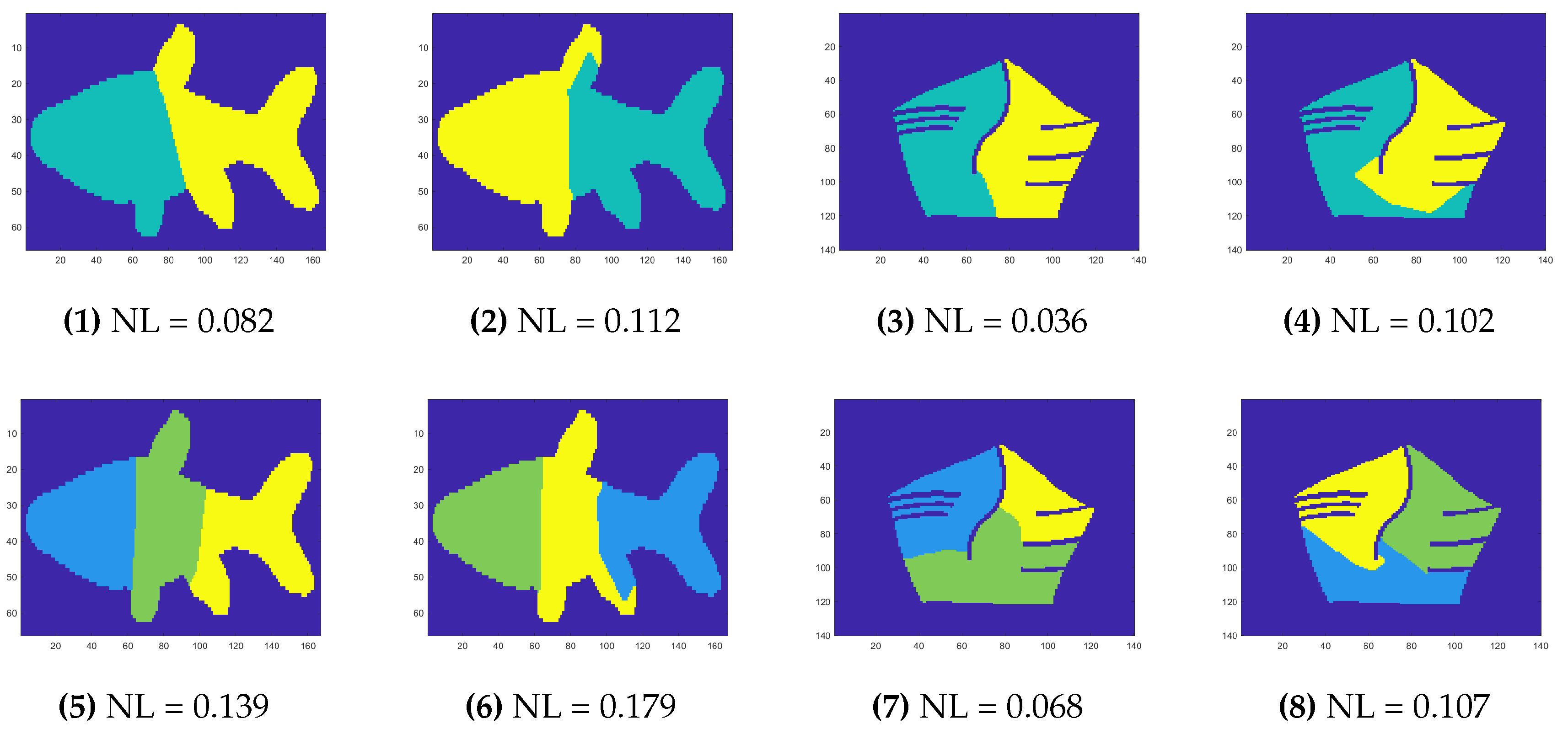
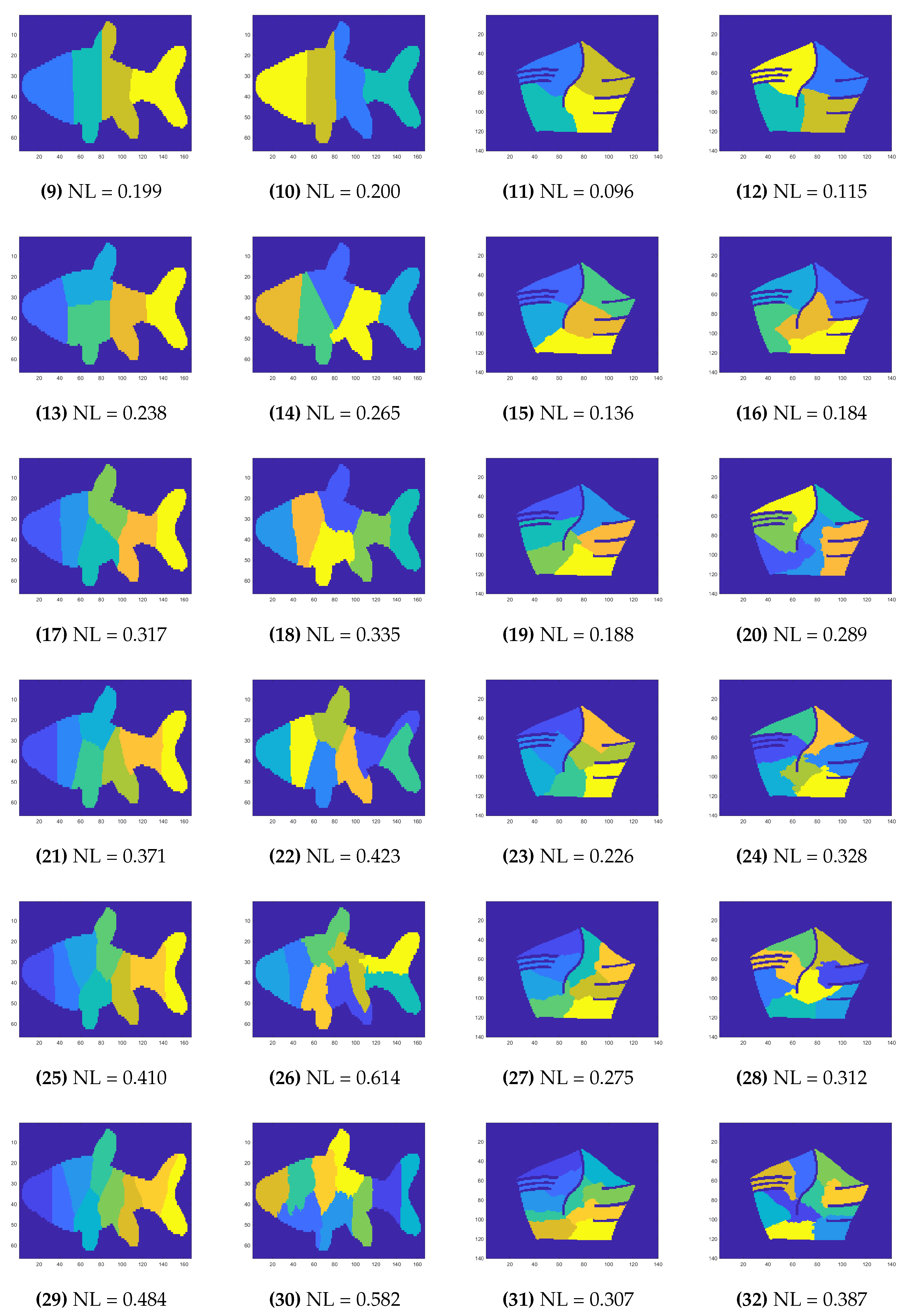
In Figure 17, we present results of SEP-PSO FBC and SEP-FBC for the two shapes of the LEMS (first two columns) and MPEG7 (last two columns) datasets with , where the outperformance of SEP-PSO FBC is maximized to show the upper limit of this outperformance. Under any value of N, it holds that SEP-PSO FBC provides better solutions in terms of metric than the corresponding solutions of SEP-FBC. In most cases, the proposed solutions of SEP-PSO FBC significantly differs from the corresponding solutions of SEP-FBC showing the importance of the selection of initial centroids, especially when a complex shape is given.
Finally, we study the sequence of the solutions derived by the proposed methods as defined in Section 6.5. Figure 14 shows the percentage of shapes in which the sequence derived by of SEP-PSO FBC and SEP-FBC does not increase monotonically, with . SEP-PSO FBC yields lower values under any dataset and N. More specifically, the mean values of this percentage of SEP-PSO FBC are 1.76 and 2.91, while the corresponding mean values of SEP-PSO are 6.69 and 7.83, under LEMS and MPEG7 datasets, respectively. This means that SEP-PSO FBC yields more robust results compared to the SEP-PSO.
Figure 14.
The percentage of shapes where the sequence is not monotonically increasing for (a) LEMS and (b) MPEG-7 datasets, with .
Figure 14.
The percentage of shapes where the sequence is not monotonically increasing for (a) LEMS and (b) MPEG-7 datasets, with .
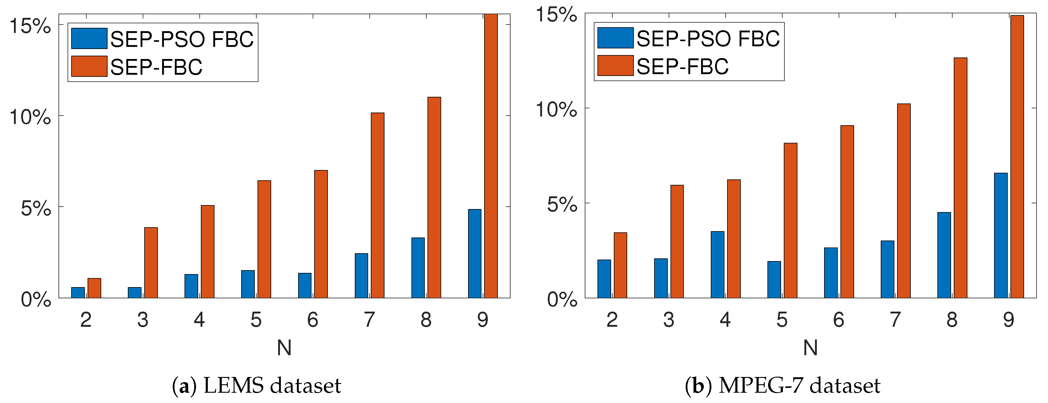
Figure 15.
The average NL metric for nine different values of of the methods SEP-PSO FBC and SEP-FBC computed on (a)-(c) LEMS and (d)-(f) MPEG7 datasets for (a) , (d) low, (b), (e) medium and (c), (f) high circularity shapes.
Figure 15.
The average NL metric for nine different values of of the methods SEP-PSO FBC and SEP-FBC computed on (a)-(c) LEMS and (d)-(f) MPEG7 datasets for (a) , (d) low, (b), (e) medium and (c), (f) high circularity shapes.
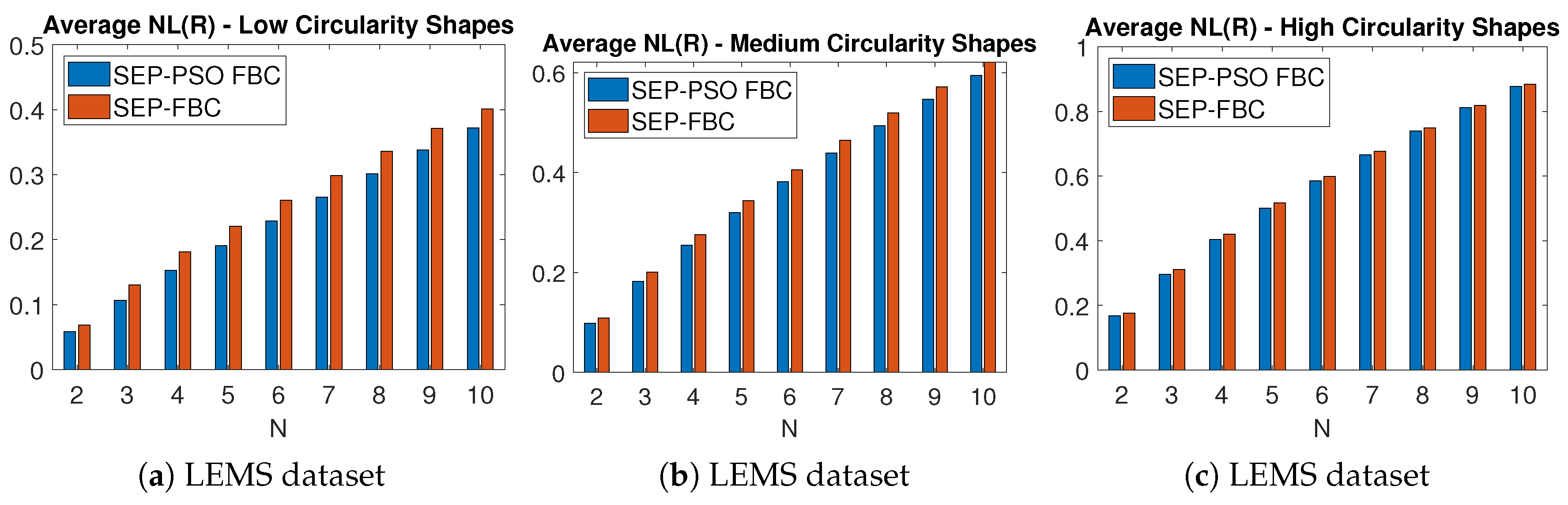
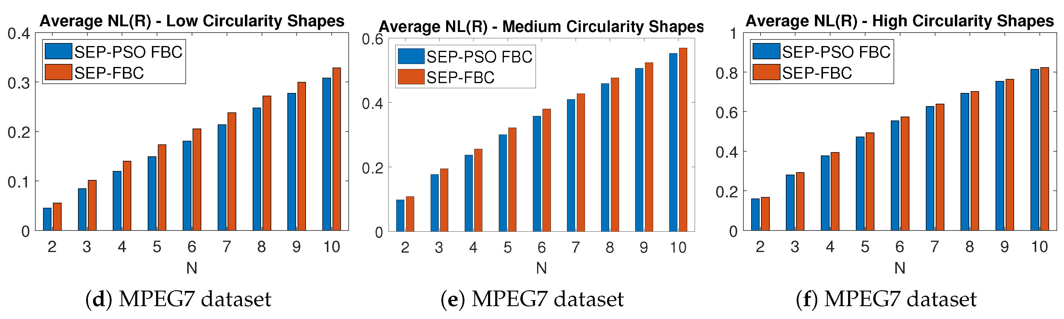
Figure 16.
Results of SEP-PSO FBC and SEP-FBC for the two shapes of LEMS (first two columns) and MPEG7 (last two columns) datasets, where the outperformance of SEP-PSO FBC is maximized.
Figure 16.
Results of SEP-PSO FBC and SEP-FBC for the two shapes of LEMS (first two columns) and MPEG7 (last two columns) datasets, where the outperformance of SEP-PSO FBC is maximized.
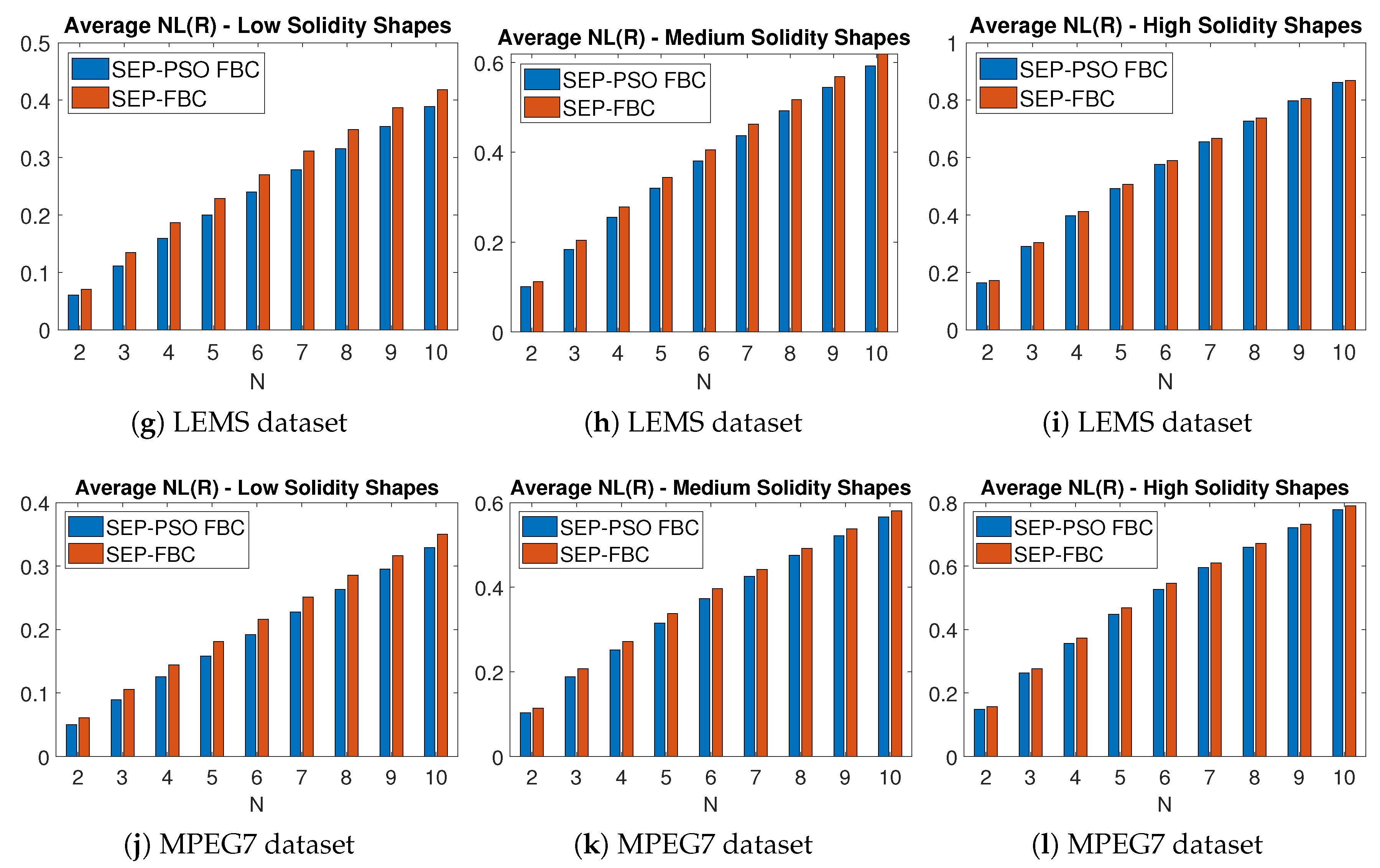
Figure 17.
A promising result of the proposed (a)SEP-PSO FBC and (b) SEP-FBC method on the tree detection problem under a low quality dense forest image.
Figure 17.
A promising result of the proposed (a)SEP-PSO FBC and (b) SEP-FBC method on the tree detection problem under a low quality dense forest image.
6.6. Applications of the Proposed Methods
The proposed methods can be applied to segmentation tasks, such as the tree detection problem [44], where the objective is to identify trees in aerial images. In cases of dense forests and low-quality imagery, unsupervised and deep learning methods often struggle to achieve accurate segmentation. Figure 18 shows a promising result of the proposed methods SEP-PSO FBC and SEP-FBC on the tree detection problem under a low quality dense forest image. In this example, even a human expert is almost impossible to detect the trees. SEP-FBC has been applied on the largest region of the bitmap image derived by RGBVI index as used in [44]. The number of trees was determined by dividing the area of the largest region by the typical size of a tree. The tree boundaries are colored blue. Under the assumption that the trees are equal sized, 188 trees were detected by the proposed methods. As expected, the of SEP-PSO FBC (2.713) is lower than that of SEP-FBC (2.806), indicating that the segmentation produced by SEP-PSO FBC is probably more preferable.
7. Conclusions
In this work, we introduced a novel methodology for the fast equipartition of complex 2D shapes, while minimizing intrinsic boundary length. The proposed method, which is based on a fast balanced clustering algorithm, demonstrates superior performance in basic shapes and outperforms existing techniques in a large number of complex shapes. Additionally, our approach is combined with the PSO framework to improve partition quality and robustness, ensuring near-optimal subdivisions even in complex shapes. Experimental results on various datasets of more than 2,800 shapes with more than more than 25,000 segmentation instances in two standard datasets, confirm the robustness and computational efficiency of our approach.
In ongoing and future work, we plan to study optimal solutions of the 2D-SEP problem with higher values of N and under more complex basic shapes. Moreover, our aim is to apply 2D-SEP on real computer vision and pattern recognition problems, where the goal is to provide segmentation of a given 2D shape. Future work could also explore extensions to three-dimensional shapes and other real-world applications.
Author Contributions
The author confirms contribution to the paper as follows: Conceptualization, C.P..; Funding acquisition, C.P.; Investigation, C.P.; Methodology, C.P.; Software, C.P.; Validation, C.P.; Supervision, G.C. and H.P.; Data Curation, C.P.; Writing – original draft, C.P.; Writing – review & editing, C.P.. C.P. reviewed the results and approved the final version of the manuscript.
Institutional Review Board Statement
Not applicable
Informed Consent Statement
Not applicable
Data Availability Statement
The associated code and datasets are developed for the project can be shared publicly after the paper acceptance. The sharing of parts of the code or datasets could be approved, at the authors’ discretion, upon request.
Conflicts of Interest
The authors declare no conflict of interest.
Appendix A
In this appendix, we study the relationship between the (8-pixel connectivity) graph-based distance , the Euclidean distance and the complete graph-based distance , as defined in Section 5, and we propose an approximation of the graph-based distance of a complete graph that combines the Euclidean distance and . Figure A1a shows examples of graph-based distances and between the point and some points (, and ) of the image space using gray and blue lines, respectively. In this example, for any pair of points it holds that the complete graph-based distance is equal to the corresponding Euclidean distance. Concerning the , it is equal to the corresponding Euclidean distances (or ) for pixels with angle , (see the white pixels in Figure A1a).
Figure A1.
(a) Examples of graph based distances and between the point and points of image space. The pixels where both distances agree are colored in white. (b) An example of graph based and the Euclidean distance between the points and in a binary image. In this example it holds that .
Figure A1.
(a) Examples of graph based distances and between the point and points of image space. The pixels where both distances agree are colored in white. (b) An example of graph based and the Euclidean distance between the points and in a binary image. In this example it holds that .
Due to the 8-pixel connectivity of the graph G, it holds that . More specifically, it holds that the ratio . This ratio is maximized for the pixels with angle (see the orange-colored pixels of Figure A1a). This direction corresponds to the bisector of the directions where the two distances are identical according to the Equation (A1). Therefore, it holds
The graph based distance of a complete graph of shape S between two points and is equal to the Euclidean distance , if and only if the points of the line segment belong to the shape S. Otherwise, it holds that . Moreover, it holds that . These distances are equal if and only if the shortest paths between the points , under two graphs are identical. Examples of such cases are shown in Figure A1b. Therefore, taking also into account the Inequality (A2), it holds that the graph based distance can be approximated by the and the as follows:
References
- Jiang, D.; Li, G.; Tan, C.; Huang, L.; Sun, Y.; Kong, J. Semantic segmentation for multiscale target based on object recognition using the improved Faster-RCNN model. Future Generation Computer Systems 2021, 123, 94–104. [Google Scholar] [CrossRef]
- Grinias, I.; Panagiotakis, C.; Tziritas, G. MRF-based segmentation and unsupervised classification for building and road detection in peri-urban areas of high-resolution satellite images. ISPRS journal of photogrammetry and remote sensing 2016, 122, 145–166. [Google Scholar] [CrossRef]
- Yi, Y.; Zhang, Z.; Zhang, W.; Zhang, C.; Li, W.; Zhao, T. Semantic segmentation of urban buildings from VHR remote sensing imagery using a deep convolutional neural network. Remote sensing 2019, 11, 1774. [Google Scholar] [CrossRef]
- Panagiotakis, C.; Argyros, A. Region-based Fitting of Overlapping Ellipses and its application to cells segmentation. Image and Vision Computing 2020, 93, 103810. [Google Scholar] [CrossRef]
- Li, H.; Zhao, X.; Su, A.; Zhang, H.; Liu, J.; Gu, G. Color space transformation and multi-class weighted loss for adhesive white blood cell segmentation. IEEE access 2020, 8, 24808–24818. [Google Scholar] [CrossRef]
- Panagiotakis, C.; Doulamis, A.; Tziritas, G. Equivalent key frames selection based on iso-content principles. IEEE Transactions on circuits and systems for video technology 2009, 19, 447–451. [Google Scholar] [CrossRef]
- Panagiotakis, C.; Tziritas, G. Any dimension polygonal approximation based on equal errors principle. Pattern recognition letters 2007, 28, 582–591. [Google Scholar] [CrossRef]
- Panagiotakis, C.; Tziritas, G. Simultaneous Segmentation and Modelling of Signals Based on an Equipartition Principle. In Proceedings of the 2010 20th International Conference on Pattern Recognition. IEEE; 2010; pp. 85–88. [Google Scholar]
- Panagiotakis, C.; Doulamis, A.; Tziritas, G. Equivalent key frames selection based on iso-content principles. IEEE Transactions on circuits and systems for video technology 2009, 19, 447–451. [Google Scholar] [CrossRef]
- Shapira, L.; Shamir, A.; Cohen-Or, D. Consistent mesh partitioning and skeletonisation using the shape diameter function. The Visual Computer 2008, 24, 249–259. [Google Scholar] [CrossRef]
- Panagiotakis, C.; Argyros, A. Parameter-free modelling of 2D shapes with ellipses. Pattern Recognition 2016, 53, 259–275. [Google Scholar] [CrossRef]
- Panagiotakis, C. The 2D Shape Equipartition Problem Under Minimum Boundary Length. In Proceedings of the International Conference on Pattern Recognition. Springer; 2024; pp. 64–79. [Google Scholar]
- Ostu, N. A threshold selection method from gray-level histograms. IEEE Transactions on systems, man, and cybernetics 1979, 9, 62. [Google Scholar]
- Preetha, M.M.S.J.; Suresh, L.P.; Bosco, M.J. Image segmentation using seeded region growing. In Proceedings of the 2012 International Conference on Computing, Electronics and Electrical Technologies (ICCEET). IEEE; 2012; pp. 576–583. [Google Scholar]
- Panagiotakis, C.; Grinias, I.; Tziritas, G. Natural image segmentation based on tree equipartition, bayesian flooding and region merging. IEEE Transactions on Image Processing 2011, 20, 2276–2287. [Google Scholar] [CrossRef] [PubMed]
- Dhanachandra, N.; Manglem, K.; Chanu, Y.J. Image segmentation using K-means clustering algorithm and subtractive clustering algorithm. Procedia Computer Science 2015, 54, 764–771. [Google Scholar] [CrossRef]
- Grau, V.; Mewes, A.; Alcaniz, M.; Kikinis, R.; Warfield, S.K. Improved watershed transform for medical image segmentation using prior information. IEEE transactions on medical imaging 2004, 23, 447–458. [Google Scholar] [CrossRef] [PubMed]
- Chan, T.F.; Vese, L.A. Active contours without edges. IEEE Transactions on image processing 2001, 10, 266–277. [Google Scholar] [CrossRef] [PubMed]
- Boykov, Y.; Veksler, O.; Zabih, R. Fast approximate energy minimization via graph cuts. IEEE Transactions on pattern analysis and machine intelligence 2001, 23, 1222–1239. [Google Scholar] [CrossRef]
- Grinias, I.; Panagiotakis, C.; Tziritas, G. MRF-based segmentation and unsupervised classification for building and road detection in peri-urban areas of high-resolution satellite images. ISPRS journal of photogrammetry and remote sensing 2016, 122, 145–166. [Google Scholar] [CrossRef]
- Minaee, S.; Wang, Y. An ADMM approach to masked signal decomposition using subspace representation. IEEE Transactions on Image Processing 2019, 28, 3192–3204. [Google Scholar] [CrossRef]
- Minaee, S.; Boykov, Y.; Porikli, F.; Plaza, A.; Kehtarnavaz, N.; Terzopoulos, D. Image segmentation using deep learning: A survey. IEEE transactions on pattern analysis and machine intelligence 2021, 44, 3523–3542. [Google Scholar] [CrossRef]
- Wang, Z.; Wang, E.; Zhu, Y. Image segmentation evaluation: A survey of methods. Artificial Intelligence Review 2020, 53, 5637–5674. [Google Scholar] [CrossRef]
- Khan, J.F.; Bhuiyan, S.M. Weighted entropy for segmentation evaluation. Optics & Laser Technology 2014, 57, 236–242. [Google Scholar]
- Panagiotakis, C. Particle Swarm Optimization-Based Unconstrained Polygonal Fitting of 2D Shapes. Algorithms 2024, 17, 25. [Google Scholar] [CrossRef]
- Lempitsky, V.; Blake, A.; Rother, C. Image segmentation by branch-and-mincut. In Proceedings of the Computer Vision–ECCV 2008: 10th European Conference on Computer Vision, Marseille, France, 12–18 October 2008; Proceedings, Part IV 10. Springer, 2008; pp. 15–29. [Google Scholar]
- Panagiotakis, C. Point clustering via voting maximization. Journal of classification 2015, 32, 212–240. [Google Scholar] [CrossRef]
- Jain, A. Data clustering: 50 years beyond K-means. Pattern Recognition Letters 2010, 31, 651–666. [Google Scholar] [CrossRef]
- MacQueen, J.B. Some Methods for Classification and Analysis of MultiVariate Observations. In Proceedings of the Proc. of the fifth Berkeley Symposium on Mathematical Statistics and Probability; 1967; Vol. 1, pp. 281–297. [Google Scholar]
- Arthur, D.; Vassilvitskii, S. k-means++: The advantages of careful seeding. In Proceedings of the Proceedings of the eighteenth annual ACM-SIAM symposium on Discrete algorithms; 2007; pp. 1027–1035. [Google Scholar]
- Theodoridis, S.; Koutroumbas, K. Pattern Recognition, 3rd ed.; Elsevier, 2006; p. 635. [Google Scholar]
- Malinen, M.I.; Fränti, P. Balanced k-means for clustering. In Proceedings of the Structural, Syntactic, and Statistical Pattern Recognition: Joint IAPR International Workshop, S+ SSPR 2014, Joensuu, Finland, 20–22 August 2014; Proceedings. Springer, 2014; pp. 32–41. [Google Scholar]
- Lin, W.; He, Z.; Xiao, M. Balanced Clustering: A Uniform Model and Fast Algorithm. In Proceedings of the IJCAI; 2019; pp. 2987–2993. [Google Scholar]
- Hales, T.C. The honeycomb conjecture. Discrete & computational geometry 2001, 25, 1–22. [Google Scholar]
- Oikonomidis, I.; Kyriazis, N.; Argyros, A.A.; et al. Efficient model-based 3D tracking of hand articulations using Kinect. In Proceedings of the BMVC; 2011; Vol. 1, p. 3. [Google Scholar]
- Farshi, T.R.; Drake, J.H.; Özcan, E. A multimodal particle swarm optimization-based approach for image segmentation. Expert Systems with Applications 2020, 149, 113233. [Google Scholar] [CrossRef]
- Papoutsakis, K.; Panagiotakis, C.; Argyros, A.A. Temporal action co-segmentation in 3d motion capture data and videos. In Proceedings of the Proceedings of the IEEE conference on computer vision and pattern recognition; 2017; pp. 6827–6836. [Google Scholar]
- Houssein, E.H.; Gad, A.G.; Hussain, K.; Suganthan, P.N. Major advances in particle swarm optimization: Theory, analysis, and application. Swarm and Evolutionary Computation 2021, 63, 100868. [Google Scholar] [CrossRef]
- Gad, A.G. Particle swarm optimization algorithm and its applications: A systematic review. Archives of computational methods in engineering 2022, 29, 2531–2561. [Google Scholar] [CrossRef]
- Kimia, B. A Large Binary Image Database, LEMS Vision Group at Brown University, 2002. http://www.lems.brown.edu/~dmc/.
- Latecki, L.J.; Lakamper, R.; Eckhardt, T. Shape descriptors for non-rigid shapes with a single closed contour. In Proceedings of the IEEE Conference on Computer Vision and Pattern Recognition. IEEE; 2000; Vol. 1, pp. 424–429. [Google Scholar]
- Bai, X.; Yang, X.; Latecki, L.J.; Liu, W.; Tu, Z. Learning context-sensitive shape similarity by graph transduction. Pattern Analysis and Machine Intelligence, IEEE Transactions on 2010, 32, 861–874. [Google Scholar]
- Zdilla, M.J.; Hatfield, S.A.; McLean, K.A.; Cyrus, L.M.; Laslo, J.M.; Lambert, H.W. Circularity, solidity, axes of a best fit ellipse, aspect ratio, and roundness of the foramen ovale: A morphometric analysis with neurosurgical considerations. Journal of Craniofacial Surgery 2016, 27, 222–228. [Google Scholar] [CrossRef]
- Markaki, S.; Panagiotakis, C. Unsupervised Tree Detection and Counting via Region-Based Circle Fitting. In Proceedings of the ICPRAM; 2023; pp. 95–106. [Google Scholar]
| 1 | The computational cost of this process is using Dijkstra algorithm with Adjacency List and Heap, since it is executed N times and the number of edges of the graph G is , due to the fact that each node of the graph has a limited number of neighbors (up to 8 neighbors). |
Figure 1.
A curve equipartition example for , .
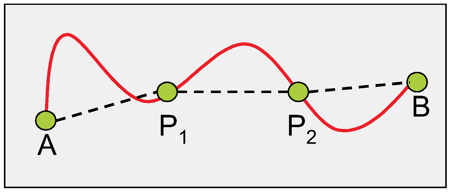
Figure 2.
Three solutions of curve equipartition problem with , are projected on the curve (blue curve) with the green color points connected with red line segments.
Figure 2.
Three solutions of curve equipartition problem with , are projected on the curve (blue curve) with the green color points connected with red line segments.
Figure 3.
Instances of the proposed 2D Shape Equipartition problem. In the first and second rows the results come from the SEP-ILS and SEP-RG methods [12] from literature, respectively. In the third row, the corresponding results come from the proposed SEP-FBC method. The number of regions (N) and the intrinsic boundary length (L) are reported in the caption of each shape.
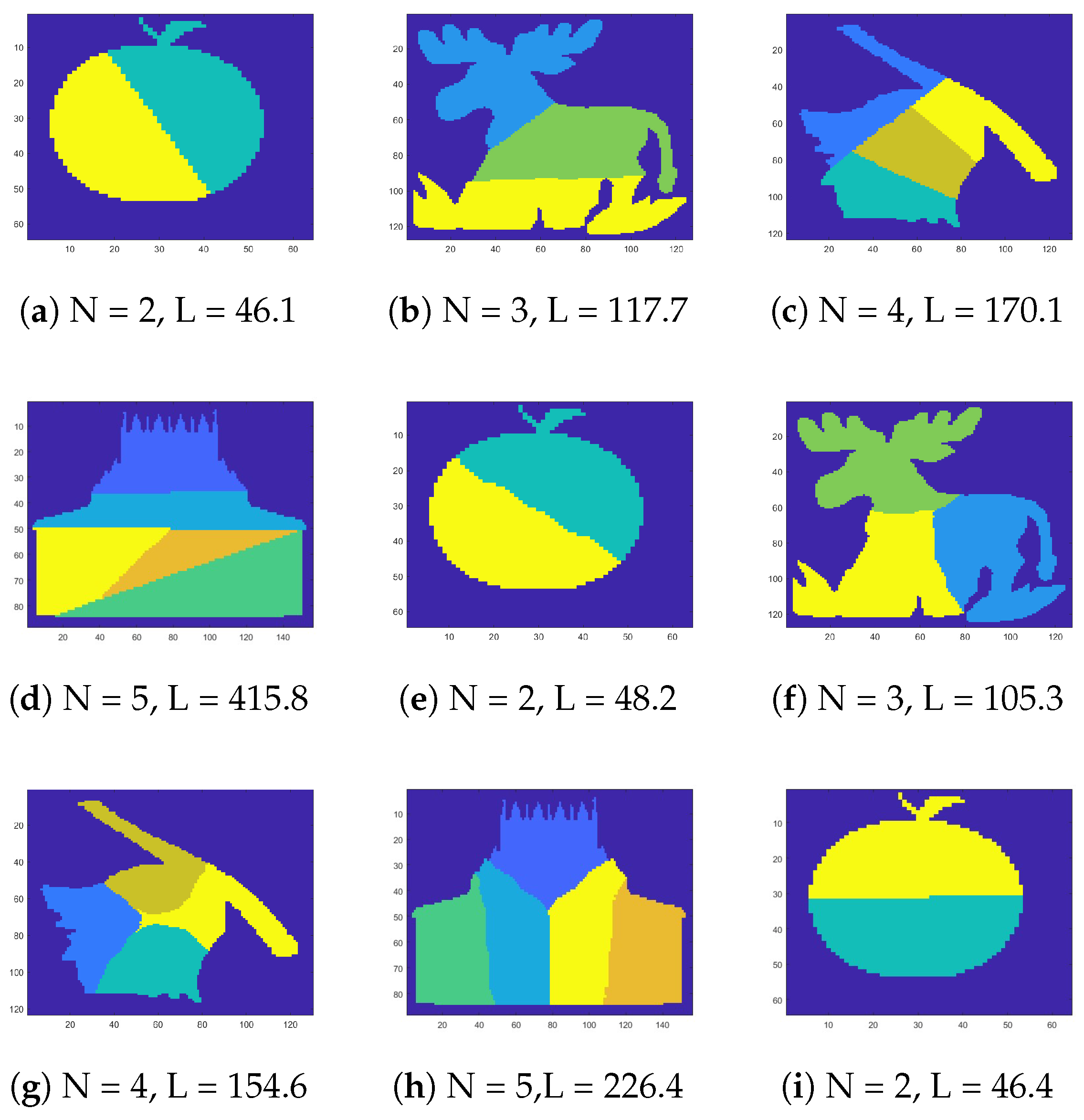
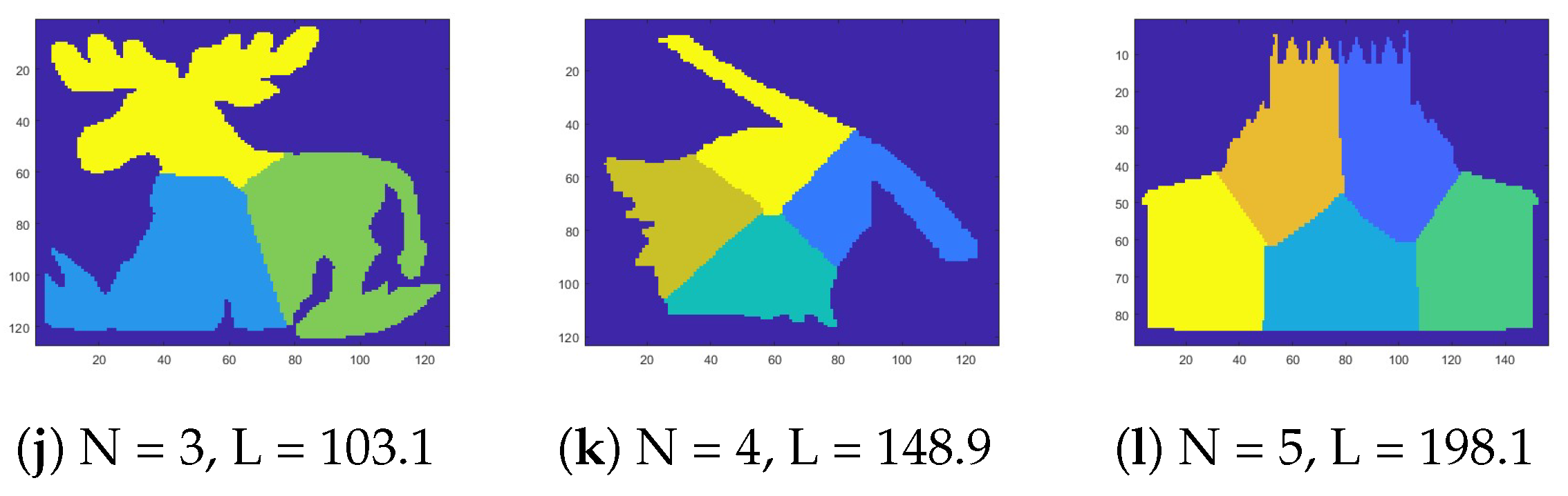
Figure 4.
Tessellations using (a) hexagons, (b) squares and (c) equilateral triangles.
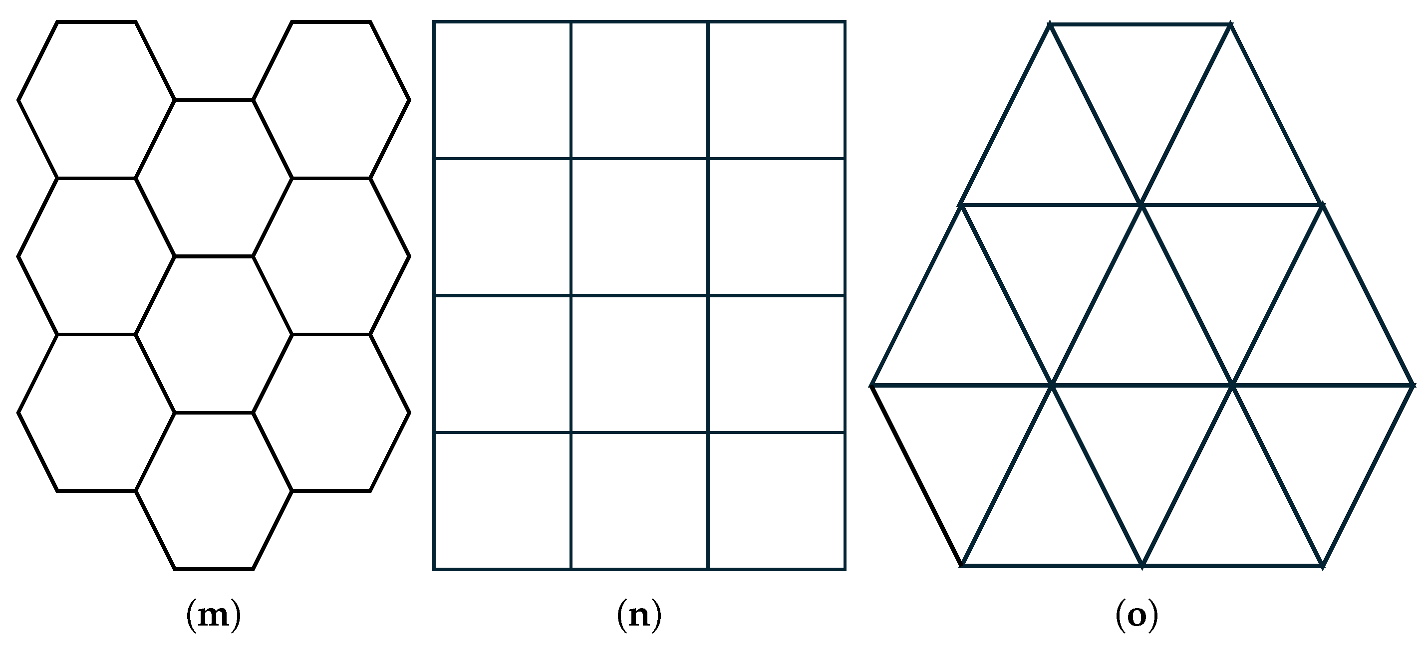
Figure 5.
Optimal solutions of the 2D-SEP for unit area ((a)-(d)) square and ((e)-(h)) circle under . The intrinsic boundary length (L) is reported in the caption of each shape.
Figure 5.
Optimal solutions of the 2D-SEP for unit area ((a)-(d)) square and ((e)-(h)) circle under . The intrinsic boundary length (L) is reported in the caption of each shape.
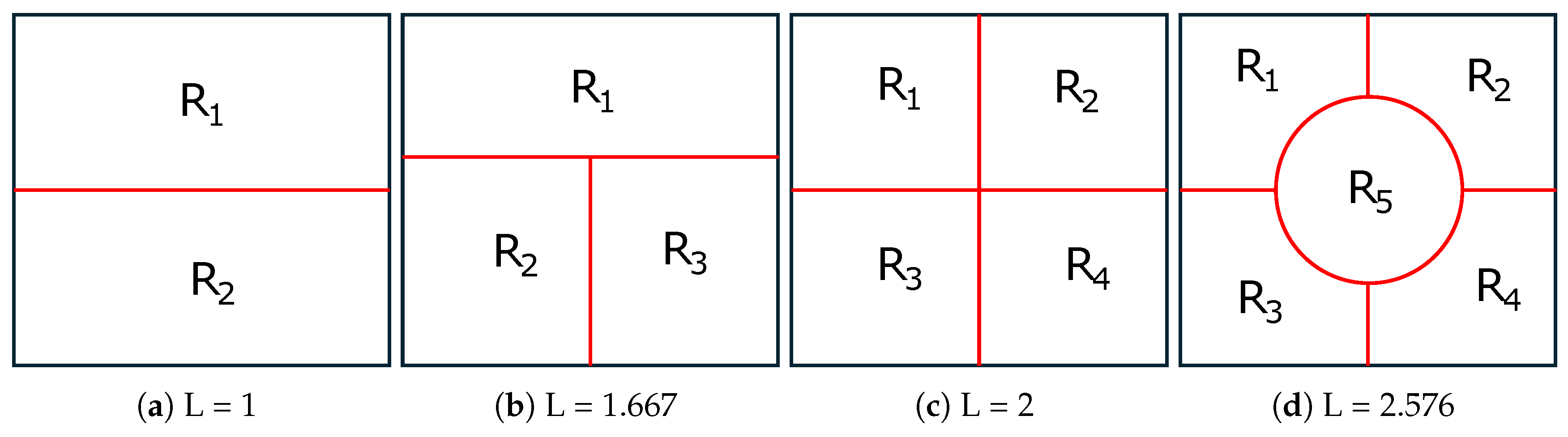
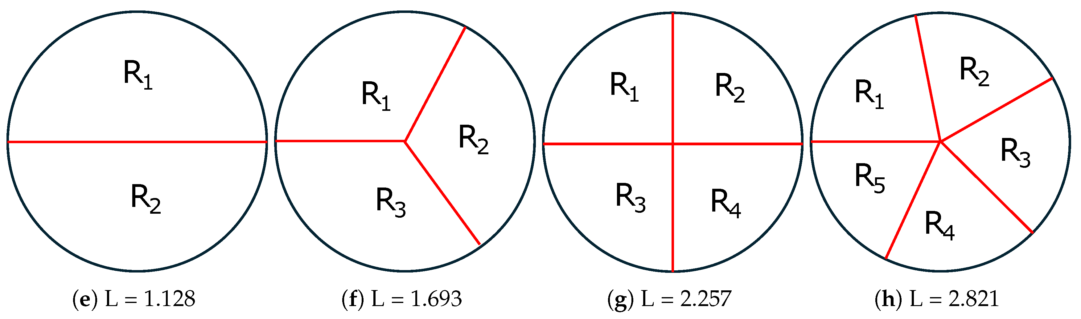
Figure 6.
Suboptimal solutions of the 2D-SEP for unit area ((a),(b)) square and ((c),(d)) circle under . The intrinsic boundary length (L) is reported in the caption of each shape.
Figure 6.
Suboptimal solutions of the 2D-SEP for unit area ((a),(b)) square and ((c),(d)) circle under . The intrinsic boundary length (L) is reported in the caption of each shape.
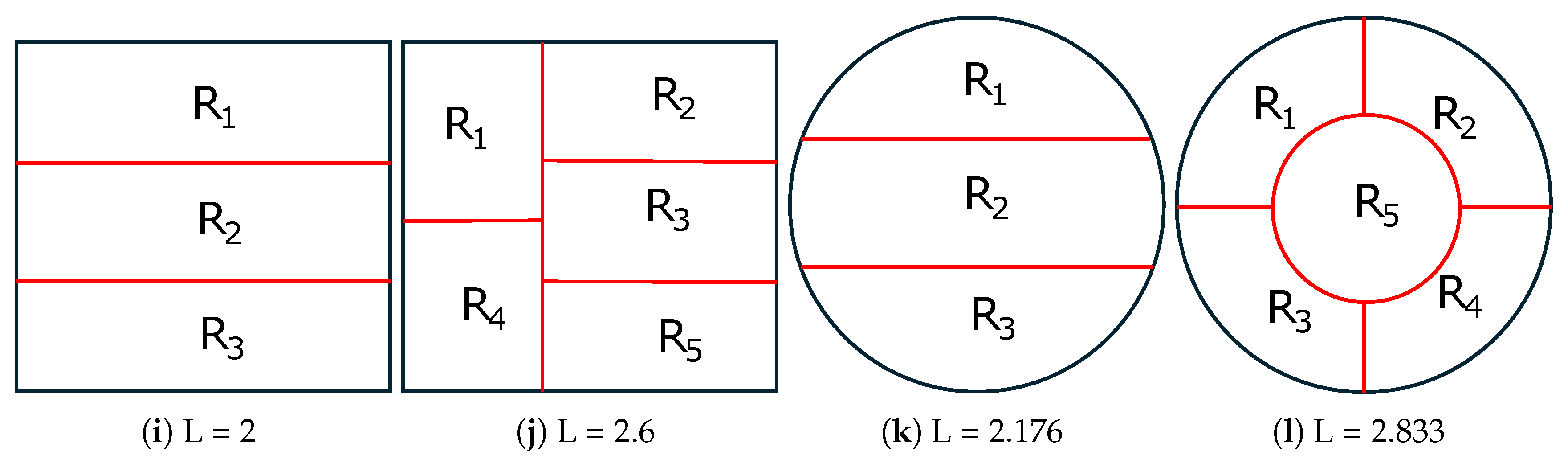
Figure 7.
Optimal solutions of the 2D-SEP for unit area ((a)-(d)) square and ((e)-(h)) circle with . The intrinsic boundary length (L) is reported in the caption of each shape.
Figure 7.
Optimal solutions of the 2D-SEP for unit area ((a)-(d)) square and ((e)-(h)) circle with . The intrinsic boundary length (L) is reported in the caption of each shape.
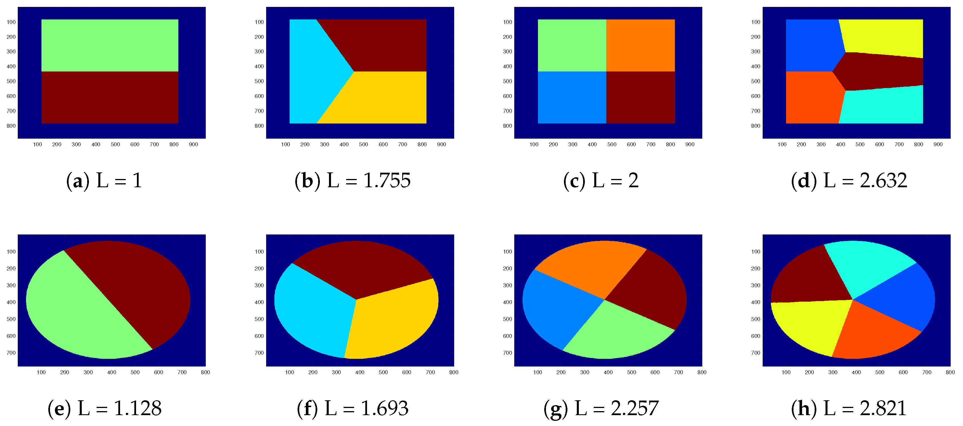
Figure 8.
A special case of shape where it holds that . The red and gree lines show the intrinsic boundary for the optimal segmentation into two and three regions, respectively.
Figure 8.
A special case of shape where it holds that . The red and gree lines show the intrinsic boundary for the optimal segmentation into two and three regions, respectively.
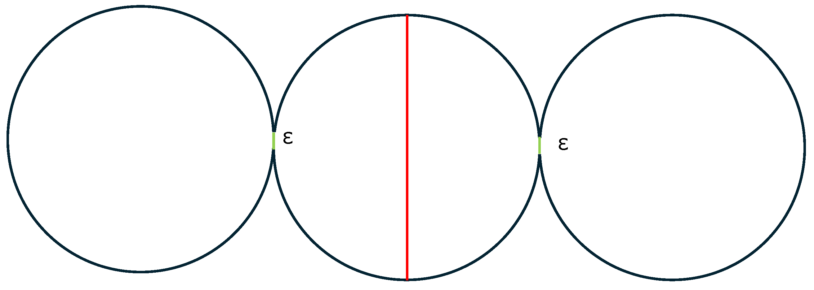
Figure 9.
Segmentation results of the two stages of the proposed SEP-FBC method for .
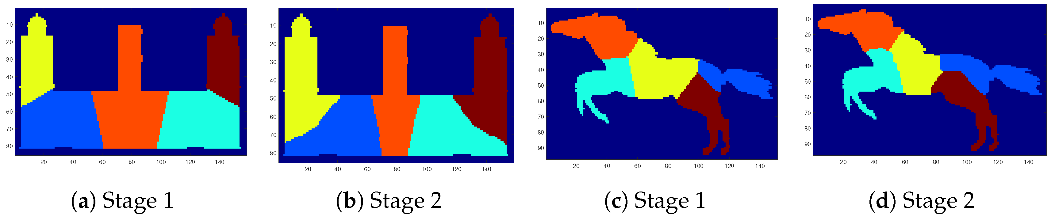
Figure 10.
Twelve sample images form (a) the LEMS dataset and (b) the MPEG-7 dataset.
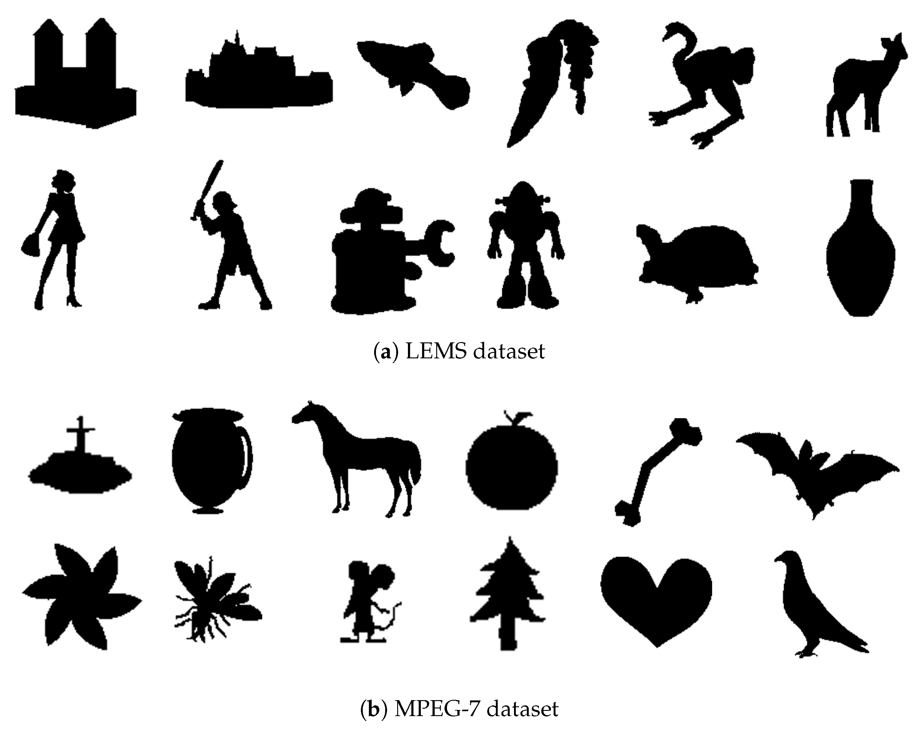
Figure 11.
The relative frequency histogram of (a) circularity and (b) solidity for the LEMS and the MPEG-7 datasets.
Figure 11.
The relative frequency histogram of (a) circularity and (b) solidity for the LEMS and the MPEG-7 datasets.
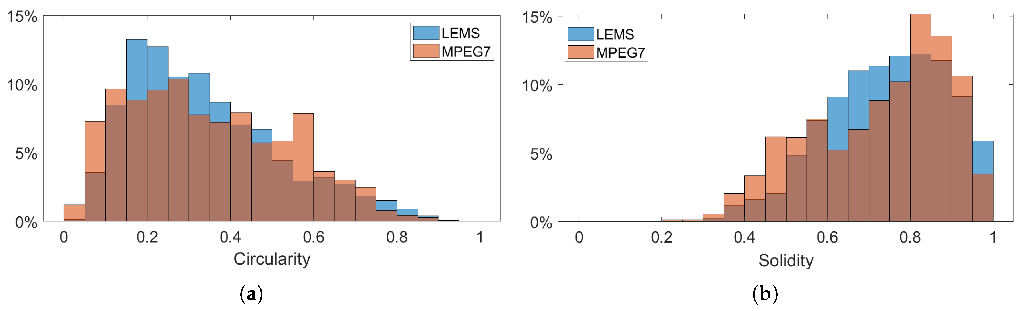
Figure 12.
The average NL metric for nine different values of of the methods SEP-PSO FBC, SEP-FBC, SEP-RG and SEP-ILS methods computed on (a) LEMS and (b) MPEG7 datasets.
Figure 12.
The average NL metric for nine different values of of the methods SEP-PSO FBC, SEP-FBC, SEP-RG and SEP-ILS methods computed on (a) LEMS and (b) MPEG7 datasets.
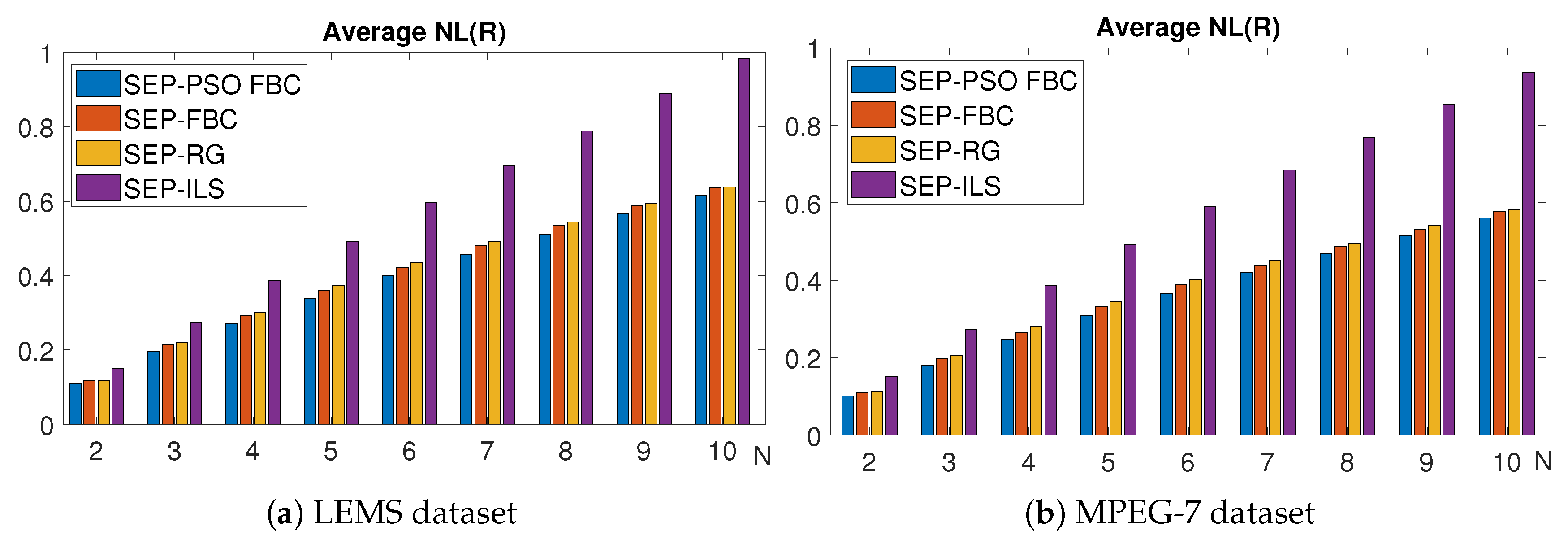
Figure 13.
The average execution time (AET) in seconds of the methods SEP-PSO FBC, SEP-FBC, SEP-RG and SEP-ILS methods computed on all images of LEMS and MPEG7 dataset.
Figure 13.
The average execution time (AET) in seconds of the methods SEP-PSO FBC, SEP-FBC, SEP-RG and SEP-ILS methods computed on all images of LEMS and MPEG7 dataset.
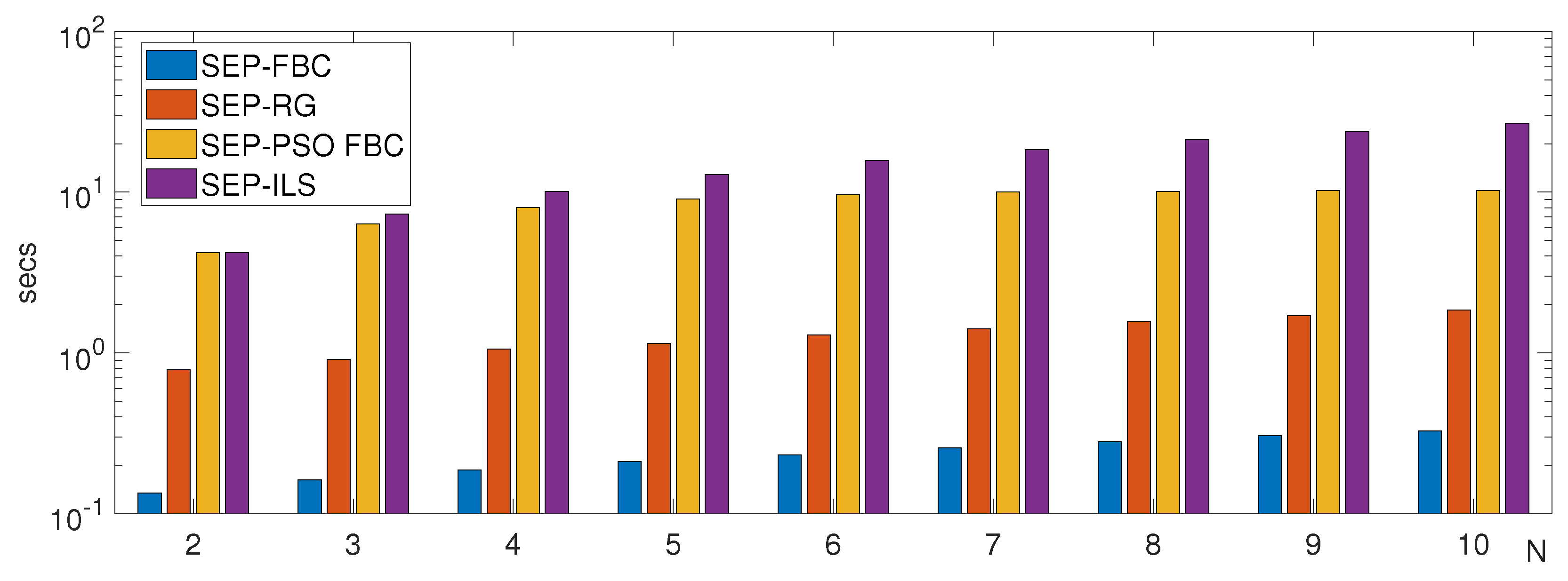
Figure 18.
A promising result of the proposed (a) SEP-PSO FBC and (b) SEP-FBC method on the tree detection problem under a low quality dense forest image.
Figure 18.
A promising result of the proposed (a) SEP-PSO FBC and (b) SEP-FBC method on the tree detection problem under a low quality dense forest image.
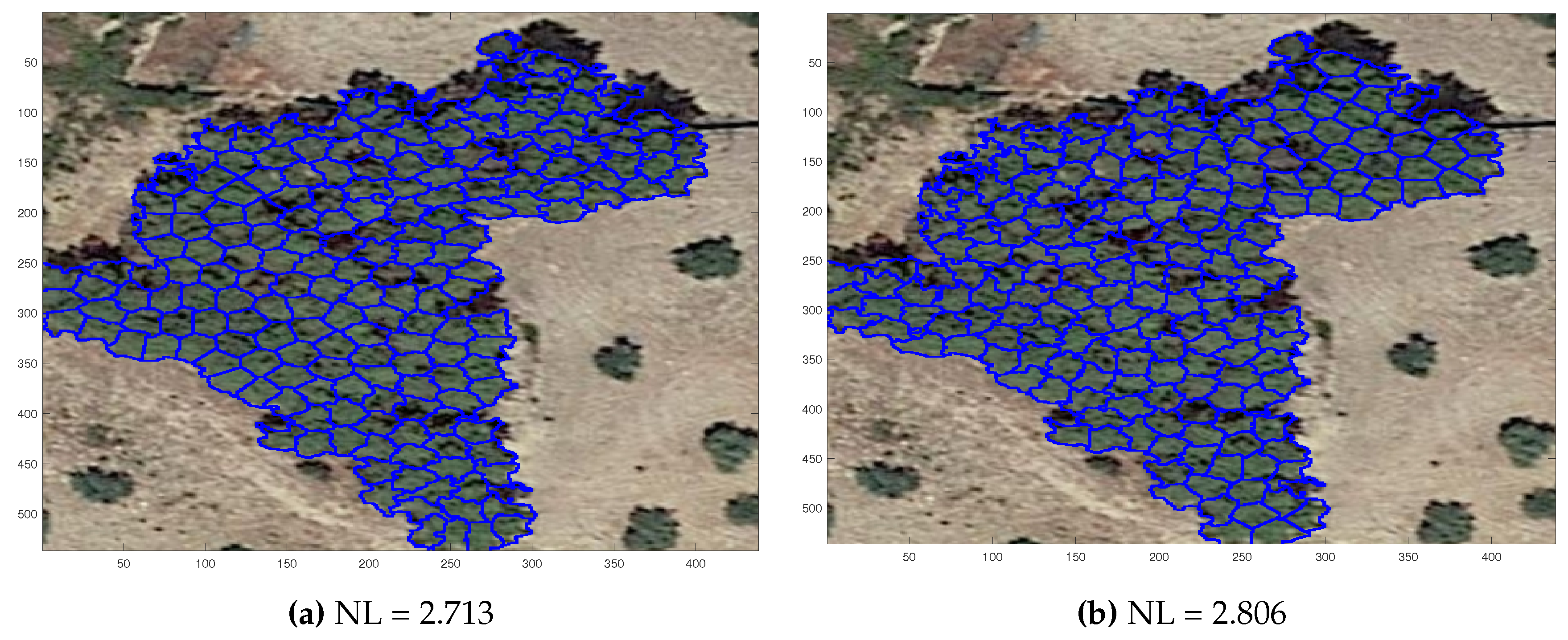

Table 1.
The perimeter of a hexagon, square and equilateral triangle as a function of its area (s).
| Shape | Perimeter |
|---|---|
| hexagon | |
| square | |
| equilateral triangle |
Table 2.
The average , and (in secs) of the methods SEP-PSO FBC, SEP-FBC, SEP-RG and SEP-ILS methods computed on all shapes of LEMS and MPEG7 dataset.
Table 2.
The average , and (in secs) of the methods SEP-PSO FBC, SEP-FBC, SEP-RG and SEP-ILS methods computed on all shapes of LEMS and MPEG7 dataset.
| LEMS Dataset | MPEG7 Dataset | |||||
|---|---|---|---|---|---|---|
| Methods | NL | Pr(m/NL) | AET | NL | Pr(m/NL) | AET |
| SEP-PSO FBC | 0.384 | 76.89% | 11.26 | 0.350 | 74.48% | 6.049 |
| SEP-FBC | 0.405 | 12.33% | 0.28 | 0.368 | 13.42% | 0.184 |
| SEP-RG | 0.413 | 8.11% | 1.46 | 0.378 | 8.46% | 1.145 |
| SEP-ILS | 0.584 | 1.12% | 21.49 | 0.572 | 0.96% | 9.727 |
Disclaimer/Publisher’s Note: The statements, opinions and data contained in all publications are solely those of the individual author(s) and contributor(s) and not of MDPI and/or the editor(s). MDPI and/or the editor(s) disclaim responsibility for any injury to people or property resulting from any ideas, methods, instructions or products referred to in the content. |
© 2025 by the authors. Licensee MDPI, Basel, Switzerland. This article is an open access article distributed under the terms and conditions of the Creative Commons Attribution (CC BY) license (http://creativecommons.org/licenses/by/4.0/).
Copyright: This open access article is published under a Creative Commons CC BY 4.0 license, which permit the free download, distribution, and reuse, provided that the author and preprint are cited in any reuse.


