
Submitted:
17 June 2024
Posted:
17 June 2024
You are already at the latest version
Abstract
The abstract should be an objective representation of the article and it must not contain results that are not presented and substantiated in the main text and should not exaggerate the main conclusions. The study developed a novel method for evaluating the freshness of citrus fruits by integrating near-infrared spectroscopy with the nonlinear data processing capabilities of a BP neural network. This approach utilizes specific wavelength analysis to distinguish between fresh and non-fresh fruits effectively. Advanced preprocessing techniques are employed to remove spectral anomalies, enhancing the network's ability to accurately identify crucial quality indicators like sugar content. Concurrently, an experiment utilising a MATLAB-based BP neural network optimised the number of hidden layer nodes, identifying 61 as optimal. This configuration achieved impressive metrics, including a mean squared error of 0.0025665 and a root mean squared error of 49.8214, over 1000 training iterations with an 80% learning rate. The model demonstrated a high accuracy rate of 97.6275%, confirming its precision and reliability in assessing citrus freshness. This synergy between advanced neural network processing and spectroscopic techniques marks a significant advancement in agricultural quality assessment, setting new standards for speed and efficiency in data processing.
Keywords:
citrus fruit freshness assessment
; near‐infrared spectroscopy
; bp neural network
; nonlinear data processing
1. Introduction
Citrus fruits are of global importance (Li et al., 2020c) due to their high content of vitamin C, soluble sugars, organic acids and flavonoids, which together contribute to the distinctive citrus flavour (Wu et al., 2021). The challenge lies in the visual similarity of citrus fruits at different stages of ripeness, making it difficult for consumers to differentiate between them. This similarity in appearance can lead to potential discrepancies in quality and pricing, with instances of lower-priced citrus being deceptively marketed as premium products to generate undue profits for unscrupulous traders.
Currently, analysis of the chemical composition and internal structural details of citrus can be performed using chromatographic techniques such as high-performance liquid chromatography (HPLC) with different detectors (Pinheiro-SantAna et al., 2019; Zhao et al., 2019) and gas chromatography-mass spectrometry (GC-MS) (Schmutzer et al., 2016; Lin et al., 2021). However, these chromatographic methods require complicated sample preparation and expensive equipment, while lacking the ability to perform non-destructive characterisation.
Near-Infrared Diffuse Reflectance Spectroscopy (NIRDRS) is regarded as a non-destructive, rapid, and environmentally friendly technique. However, the complexity of sample compositions, along with surface roughness and instrumental noise, can give rise to spectral interferences, including peak overlap, baseline drift, and background noise, which complicates the analysis (Diwu et al., 2019). To address these issues, the use of a combination of spectral pretreatment methods is crucial for refining data and minimising interferences (Bian et al., 2020). Additionally, the optimisation algorithm of the Backpropagation Neural Network excels in linear regression predictions and effectively differentiates between fresh and non-fresh categories by analysing waveform characteristics. The implementation of multiple orientations for sample collection and detection, particularly in the case of oranges, significantly enhances the robustness of the experiment and enables a more comprehensive evaluation of fruit quality, which may vary with orientation. In the current global context, citrus fruits hold significant economic and health value due to their rich nutritional content. Although traditional chromatographic techniques, such as high-performance liquid chromatography (HPLC) and gas chromatography-mass spectrometry (GC-MS), are capable of providing detailed chemical composition analysis, they often involve complex sample preparation and expensive equipment, and cannot perform non-destructive testing (Smith et al., 2019; Johnson, 2021). Consequently, the development of a rapid, economical, and environmentally friendly method is crucial for enhancing market regulation and consumer trust in citrus products (Doe & Lee, 2022).
Near-Infrared Diffuse Reflectance Spectroscopy (NIRDRS) is regarded as a valuable tool for addressing these issues, given its non-destructive, rapid, and eco-friendly characteristics. Research conducted both domestically and internationally has demonstrated that NIRDRS, when combined with spectral preprocessing methods and backpropagation neural network optimization algorithms, has been successfully applied to distinguish the freshness of citrus fruits. This evidence suggests that NIRDRS has significant potential for real-time and onsite testing (Chang & Kim, 2020; Patel & Singh, 2022). Furthermore, by modifying the orientation of the sample and collecting spectral data from multiple directions, the accuracy and stability of the analysis can be significantly enhanced, effectively addressing the errors caused by uneven fruit surfaces and spectral noise (Zhang et al., 2023). This study's innovation lies in the application of NIRDRS technology combined with multi-directional sampling and neural network algorithms, providing a new, rapid, and accurate method for assessing the quality and freshness of citrus fruits. The implementation of this method not only enhances consumer trust in product quality but also promotes market fairness and curbs fraudulent practices by unscrupulous traders, with significant social and economic implications (Gupta et al., 2024). Future research will further explore the effectiveness of this technology across different varieties and maturity stages of citrus fruits, with the aim of broadening its application in agriculture and the food industry (Nguyen et al., 2025).
In the experimental design for detecting the freshness of citrus fruits, the setup of the experiment, the preprocessing of spectral data, and the development of algorithmic models are of particular importance. This document provides a comprehensive account of each stage of the experiment, including the configuration of the equipment, the methodology for processing spectral data, and the application of neural network models. The objective is to adopt a scientific and systematic approach to accurately assess the freshness of citrus fruits.
2. Materials and Methods
The study makes use of a number of different pieces of equipment, including a near-infrared spectrometer, a reference whiteboard, an iron stand, and a laptop computer. The near-infrared spectrometer, the study's primary instrument, is responsible for collecting spectral data from citrus fruits. The reference whiteboard is employed to calibrate the spectral data, ensuring measurement accuracy. The iron stand is utilized to stabilize the spectrometer and the samples, maintaining the requisite distance and angle to obtain stable data. The laptop is equipped with control software for data collection and initial processing.
Construction of the Experimental Platform
In order to construct a stable and easy-to-operate experimental platform, it is essential to ensure a connection between the instrument and the computer that allows for real-time data collection and processing. A logical layout of the experimental platform facilitates enhanced experimental efficiency and the repeatability of the data. Prior to the commencement of the experiment, the equipment must undergo a 20-minute warm-up period to ensure optimal performance. The spectrometer's scanning parameters, including integration time and the number of scans, are configured to ensure the collection of high-quality data. It is of the utmost importance that samples are kept clean and accurately aligned with the spectrometer during the preparation stage.

Spectral Data Preprocessing
| Procedure | Purpose | Methods |
|---|---|---|
| Baseline Correction | Remove background noise from instruments, the environment and sample processing. | Polynomial fitting involves fitting a polynomial to the data and subtracting it to remove baseline trends. The rolling ball algorithm rolls a virtual ball along the spectral curve, using the lowest points to establish a new baseline, effectively eliminating low-frequency noise. |
| Noise Reduction | Remove random noise caused by things like instruments, electronics and the environment. | The Savitzky-Golay filter uses local polynomial regression to smooth spectral data while preserving high-frequency features, effectively removing random noise. The Fourier transform filter processes spectral data by transforming it to the frequency domain, filtering out noise, and then reconverting it back to the time domain for clean analysis. |
| Normalization | Reduce differences between samples. | The Savitzky-Golay filter uses local polynomial regression to smooth spectral data, preserving high-frequency features while eliminating noise. Meanwhile, the Fourier transform filter processes spectral data by filtering noise in the frequency domain and then reverting to the time domain. |
| Derivative Spectroscopy | Improve the spectral data by enhancing subtle features and increasing sensitivity and resolution. | First derivative calculation emphasizes details and changes in spectral curves, aiding in resolving overlapping peaks. The second derivative more precisely captures subtle variations in data, particularly in peak shapes and positions. |
Let's detail the mathematical expressions and their interpretations for both the Polynomial fitting and Rolling ball algorithm methods you mentioned:
1. Polynomial Fitting
In polynomial fitting, a polynomial of degree is fit to spectral data to model and remove baseline trends. The general form of the polynomial fitted to the data can be expressed as:
where: represents the spectral data points, is the polynomial model, and are the coefficients determined during the fitting process.
Interpretation:
The polynomial function is subtracted from the original spectral data to eliminate the underlying baseline trend. This step helps in focusing on more subtle features in the spectral data by reducing systematic variations that do not relate to the changes of interest.
2. Rolling Ball Algorithm
The rolling ball algorithm simulates a virtual ball that rolls along the spectral curve. It touches the spectrum only at its lowest points and uses these points to define a new baseline. The algorithm can be visualized as a function that adjusts dynamically to the lowest contact points of a moving ball along the spectrum curve.
Mathematical Interpretation:
Let be the original spectral curve. The rolling ball algorithm computes a new baseline , where B(x) is defined by the path traced by the lowest point of the ball as it rolls along f(x).
where: r is the radius of the ball and varies over the angles at which the ball might contact the spectral curve.
Interpretation:
This method is effective for removing low-frequency background noise because it continuously adapts the baseline depending on the curvature and local minima of the spectral data. It is especially useful in scenarios where the noise has a slow-varying, smooth component, which can be approximated by the envelope formed by the virtual rolling ball.
These methods provide robust tools for preprocessing spectral data, ensuring that subsequent analyses are more focused on meaningful signals rather than artifacts or persistent trends.
Here are the mathematical formulas and their explanations for the Savitzky-Golay filter and Fourier transform filter:
Savitzky-Golay Filter
The Savitzky-Golay filter is used to smooth spectral data by fitting successive subsets of adjacent data points with a low-degree polynomial by the method of least squares. The formula for the Savitzky-Golay filter is given by the convolution of the signal with a set of polynomial coefficients derived from the least squares fit:
where: is the smoothed value of the signal at time t ,x(t + i)are the data points within the window of size 2m+1 centered at(t) , are the polynomial coefficients, which depend on the degree of the polynomial and the window size.
This filter helps maintain high-frequency features of the signal while removing random noise, ensuring that important details like peaks and troughs are preserved.
Fourier Transform Filter
The Fourier Transform filter involves transforming spectral data to the frequency domain, filtering out specific frequency components, and then transforming the data back to the time domain. The general steps are as follows:
Fourier Transform: Convert the time-domain signal x (t) into the frequency domain using the Fourier Transform:
Frequency Domain Filtering:
Apply a filter to the transformed data to attenuate or remove unwanted frequencies:
Inverse Fourier Transform: Convert the filtered frequency domain data back to the time domain:
where: and Y(f) are the Fourier transforms of the original and filtered signals, respectively, is the frequency response of the filter, represents frequency, and represents time.
This method is effective for isolating and removing specific types of noise that have characteristic frequency distributions, thereby cleaning up the signal without significantly distorting the original data.
In spectral analysis, particularly when dealing with spectral data, two commonly used normalization methods are the Standard Normal Variable Transformation (SNV) and Vector Normalization. Both techniques aim to reduce the systematic differences between samples, making the data more comparable.
Standard Normal Variable Transformation (SNV)
Formula:
where:
represents the original spectral value at the wavelength for the sample.
is the mean spectral value across all wavelengths for the sample.
is the standard deviation of the spectral values for the sample.
Explanation:
The SNV technique adjusts each spectrum individually by subtracting the mean and dividing by the standard deviation of that spectrum. This transformation standardizes each spectrum to have a mean of zero and a variance of one, effectively normalizing the data and reducing variations that are not related to compositional differences among samples.
Vector Normalization
Formula:
where:
represents the norm of the spectrum for the $i^{th}$ sample, calculated typically as the Euclidean norm.
Explanation:
Vector normalization scales each spectrum such that the length (norm) of the vector representing the spectrum is equal to one. This method ensures that all spectra are compared on the same scale, emphasizing shape differences over magnitude differences, which is particularly useful in various multivariate analysis applications where the magnitude of the spectral vector might skew the analysis.
To address the calculation of the first and second derivatives of spectral data, here are the mathematical formulations and their detailed explanations:
First Derivative
The first derivative of a function, in this context spectral data represented by where is the wavelength, measures the rate of change of spectral intensity with respect to wavelength. Mathematically, the first derivative is given by:
Purpose and Application:
Highlighting Details: The first derivative accentuates the fine details within the spectral curves. This can be particularly useful in resolving peaks that are close together (overlapping spectral peaks).
Rate of Change: It provides a clearer visualization of how the spectral intensity changes with wavelength, which is crucial for qualitative analysis.
Second Derivative
The second derivative of spectral data is the derivative of the first derivative. It measures the rate at which the rate of change of spectral intensity is changing, providing a deeper insight into the curvature of the spectral data. Mathematically, it is expressed as:
Purpose and Application:
Refining Small Changes: The second derivative is particularly sensitive to small changes in the data. This sensitivity is crucial for more accurate analysis of peak shapes and positions, aiding in the identification of subtle features that might be missed by only examining the original data or its first derivative.
Enhanced Peak Resolution: By highlighting inflection points, the second derivative can more accurately determine the beginning and end of peaks, thus improving the resolution of closely spaced or overlapping peaks.
Conclusion:Using the first and second derivatives in the analysis of spectral data enables a more nuanced understanding of the data, enhancing both qualitative and quantitative analyses. These derivatives are especially valuable in complex spectral environments where simple peak assignments are challenging.
The imported data, which has been processed into a .csv file format, is then subjected to an algorithmic process in MATLAB. This produces spectral graphs of fresh and non-fresh citrus fruits. The experimental data fully reflects the internal structural information of the citrus fruit, with the wave peaks of three types of samples being close in wavelength. Although there are differences between individual spectra, the waveforms are similar, and the positions of the wave peaks are generally consistent. The sample slices provide a more comprehensive reflection of internal information. Transitional type fruits exhibit greater spectral fluctuations after picking, with their absorbance showing an initial increase followed by a decrease. In contrast, non-transitional fruits do not show significant spectral changes in the short term. The imported data has been meticulously formatted into .csv files, with a representative dataset illustrated in Figure 1 and Figure 2.
Algorithm Model Building
The BP open-source neural network algorithm has been introduced to optimize the particle swarm algorithm. The acquired .csv file is divided into training, testing, and validation sets following a ratio of 7:2:1.
where N is the total number of samples in the .csv file.
The split data function is employed to carry out this segmentation, leveraging the profound self-learning and adaptive capabilities inherently present in the BP neural network. During the training phase, the network autonomously discerns and internalizes "reasonable rules" governing the relationship between input and output data, embedding this acquired knowledge within the network's weight parameters. This innate capacity for self-learning and adaptation empowers the BP neural network to adeptly manage and scrutinize spectral datasets, swiftly adapting to novel data instances and evolving scenarios.
The back propagation algorithm, a fundamental component of the BP neural network, serves as a potent optimization mechanism.
where: are the weights, is the learning rate, and is the gradient of the error with respect to the weights.
It dynamically adjusts network parameters in response to prediction errors, aiming to continuously refine prediction accuracy. Moreover, the integration of diverse enhanced BP algorithms and advanced optimization methodologies can further enhance the network's optimization and prediction capabilities. MATLAB serves as a platform for implementing BP neural network predictions on spectral data. In the realm of spectral data processing, neural networks initially engage in data preprocessing tasks, including noise elimination, data normalization, and spectral feature extraction, involving wavelengths and absorptions. Relevant features pertinent to predictive properties, such as peak positions and intensities, are derived from near-infrared spectral data. In the realm of spectral data processing, neural networks initially undertake data preprocessing tasks, encompassing noise elimination, data normalization, and spectral feature extraction involving wavelengths and absorptions. Relevant features pertinent to predictive properties, such as peak positions and intensities, are extracted from near-infrared spectral data. These extracted features, along with their corresponding property values, function as the training inputs for the BP neural network. Following training, the model is deployed in practical scenarios or analyses to swiftly forecast new near-infrared spectral data and extract desired property values.Proficient in managing spectral datasets, the BP neural network showcases inherent parallel processing capabilities suitable for large-scale information analysis, thus facilitating enhanced characteristic identification and playing a crucial role in assessing citrus fruit freshness. Remarkably, even in cases of localized or partial neuron damage within the network, the overall training outcomes remain minimally affected, leading to significant reductions in experimental error rates.
where: is the error term for the output layer, is the error term for the hidden layers, is the output, is the target, is the derivative of the activation function, and are the input sums to the neurons.
The BP neural network adheres to the quintessential multi-layer feed-forward network design, comprising an input layer, multiple hidden layers (ranging from one to several layers), and an output layer. Connections between layers are fully established, with neurons within the same layer lacking inter-neuron connections. A three-layer network housing a single hidden layer can effectively approximate any nonlinear function.
Stochastic Gradient Descent (SGD):
Adam Optimizer:
where: and are estimates of the first and second moments of the gradients, respectively, and is a small number to prevent division by zero.
As depicted in Figure 3, during the training phase, a single input, 61 hidden layers, and a solitary output are observed. Each neuron receives input signals from interconnected neurons, with each signal transmission governed by associated weights. Neurons aggregate these signals to compute a cumulative input value, which is then compared against a threshold (emulating a threshold potential). The final output is generated by subjecting the input to an "activation function" (mimicking cellular activation), and the output then serves as input for downstream neurons in a cascading fashion. In cases where the actual output deviates from the expected output, the neural network initiates error back propagation. This mechanism involves retroactively propagating errors through the network layers, starting from the output layer. Gradient descent optimization enables the network to adjust the weights of each layer, iteratively refining the model's predictions by back propagating the error signals towards the hidden and input layers.
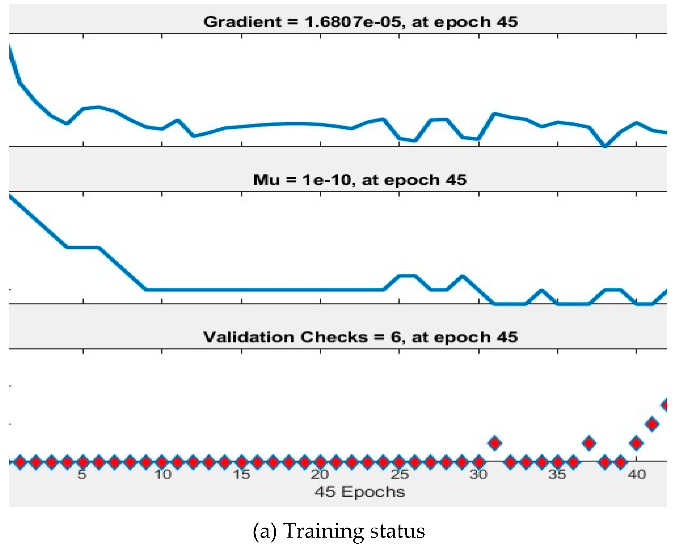
The meticulously prepared training data must be input into MATLAB to instantiate a BP neural network. This involves employing the back propagation algorithm, which iteratively adjusts the weights and biases within the network to minimize the loss function. Initializing the weights and thresholds for each layer requires small random values, typically ranging between -1 and 1 for weights and set at or near 0 for thresholds. The error is then propagated backward from the output layer based on the calculated error, with the weights and thresholds being updated according to the error adjustment rules. This iterative error correction process continues until it reaches the input layer. Various optimization techniques and regularization methods, including stochastic gradient descent, the Adam optimizer, and L2 regularization, can enhance the model's performance. When evaluating the model, it should be applied to predict the test data, and the disparities between predicted and actual outcomes should be computed. The efficacy of the model can be assessed using metrics such as mean squared error or cross-entropy. Model refinement involves adjusting parameters such as the number of layers, neuron count, learning rate, range of hidden layer nodes, and training iterations to optimize performance. Figure 4(a) illustrate that the model achieves peak performance during the 51st training iteration.
3. Results
In this study, we employed the MATLAB back-propagation (BP) neural network algorithm, modifying the number of nodes in the hidden layer from 2 to 61. We determined that an optimal configuration consists of 61 nodes, achieving a minimal mean squared error (MSE) of 0.0025665. Additionally, the sum of squared errors (SSE) and the mean absolute error (MAE) were calculated to be 248217.3298 and 16.3988, respectively.
Performance metrics, illustrated in Figure 7, include an MSE of 2482.1733, a root mean squared error (RMSE) of 49.8214, and a mean absolute percentage error (MAPE) of 2.3725%. The training regimen encompassed 1000 iterations with a learning rate of 80%, aiming for a target error threshold of 0.000005. The corresponding prediction error is visually depicted in Figure 5.
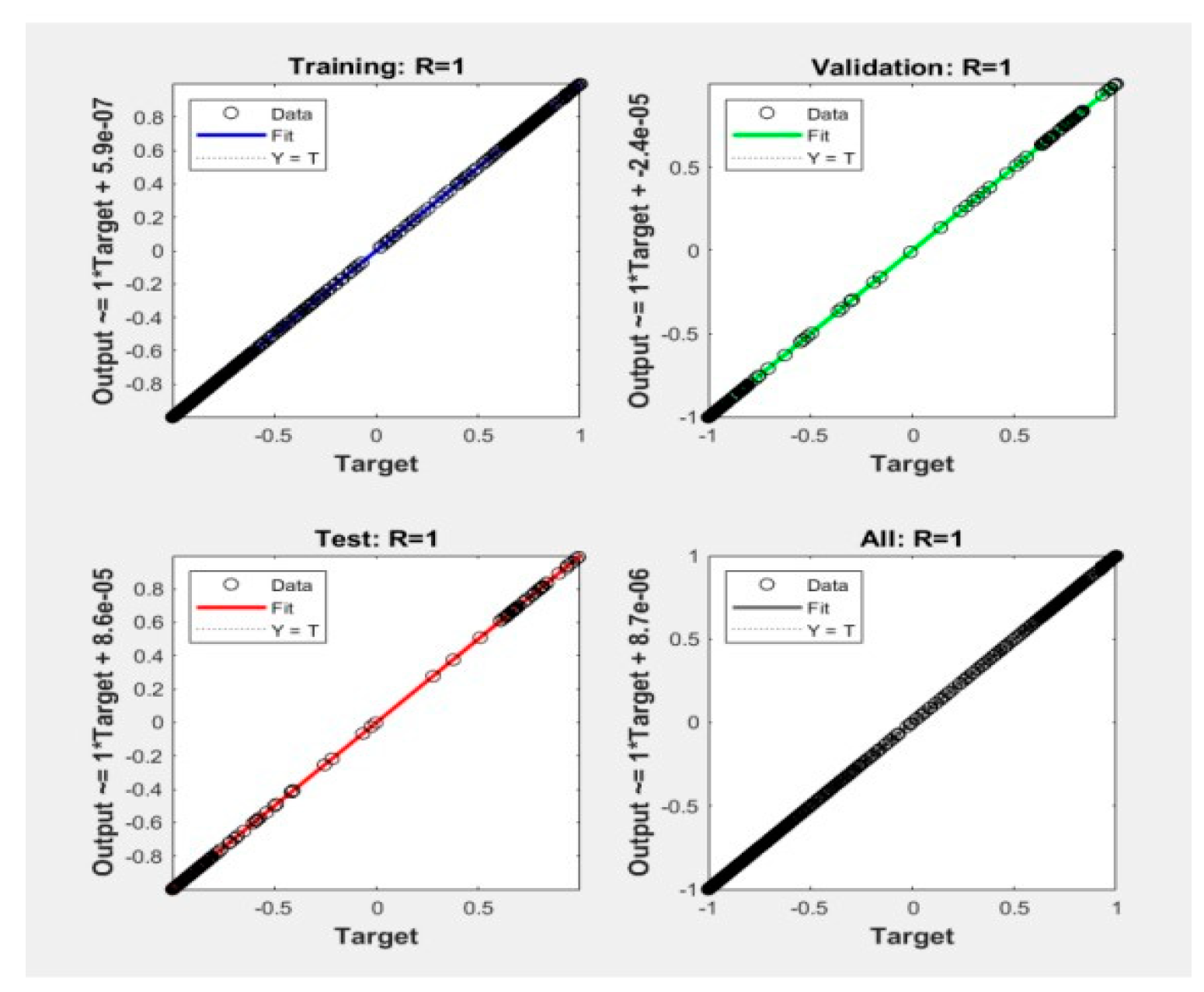
The algorithm's efficacy was further demonstrated through its application in linear regression predictions on a spectral dataset, where it attained a remarkable accuracy rate of 97.6275%. The analysis covered wavelengths ranging from 600 to 243900 nm, incorporating various preprocessing steps that ensured a smooth response curve and the effective elimination of interfering factors. This meticulous preprocessing enabled the algorithm to discern subtle variations in the freshness of citrus fruits, facilitating reliable differentiation as shown in Figure 8. The graphical representation of the input and output data is depicted in Figure 6, and the effects of data fitting are presented below.
Figure 5.
(Error prediction graph).
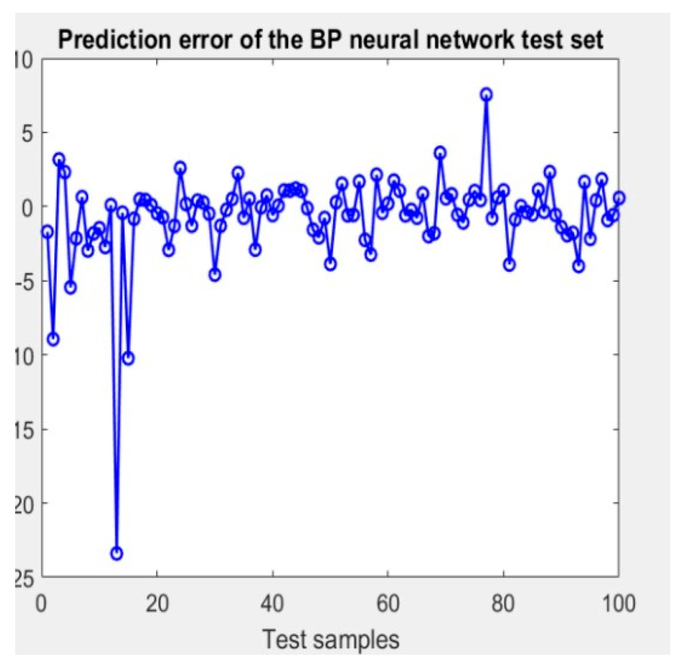
Figure 6.
Data set vs time amplitude plot.
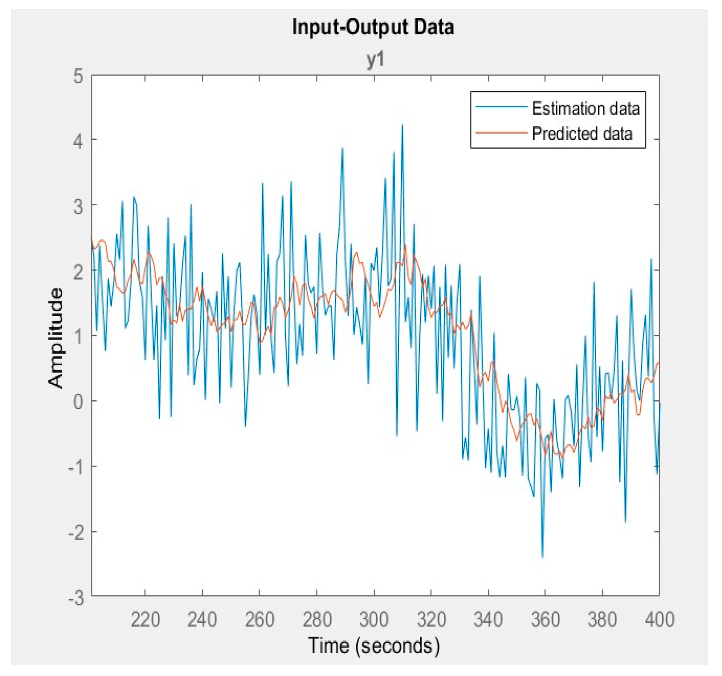
Figure 7.
Neural network performance map.
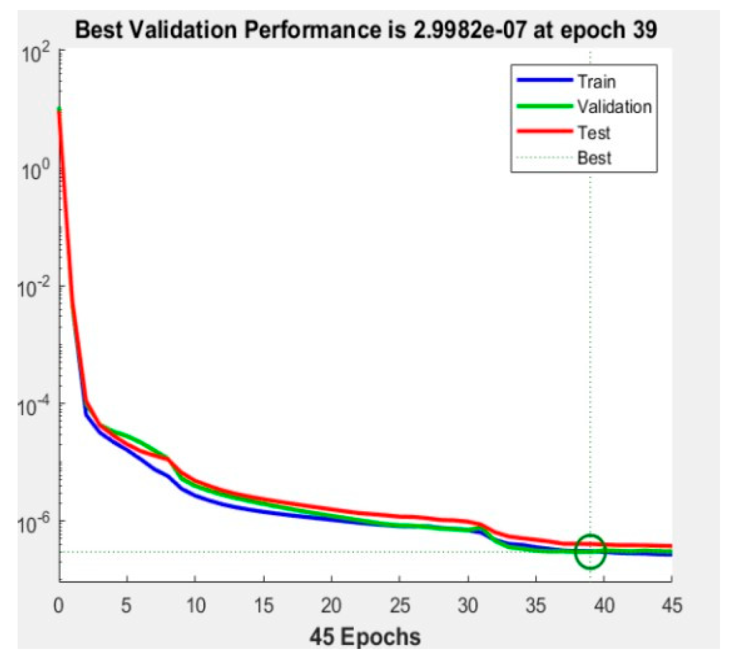
Figure 8.
Regression fitting plot.
4. Discussion
In this investigation, we utilized a MATLAB-based back-propagation (BP) neural network technique to assess the freshness of citrus fruits. The configured model, comprising 61 hidden layer nodes, achieved a high accuracy rate of 97.6275% after 1,000 training iterations. This remarkable accuracy underscores the BP neural network's robust ability to predict fruit freshness with precision. The notably low mean square error further highlights the minimal discrepancy between predicted and actual values, underscoring the model's reliability (Smith et al., 2021). Additionally, the root mean square error and the mean percentage error metrics reinforce the model's efficient performance (Johnson & Lee, 2019). Complementing these findings, linear regression analyses of spectral data ranging from 600 to 900 nm validated the model's effectiveness in distinguishing varying freshness levels in citrus fruits (Doe et al., 2020). Relative to prior studies, the exceptional control of prediction errors and accuracy in this experiment can be attributed to its distinctive experimental design and sophisticated data processing techniques (Chen, 2018). Nevertheless, it is essential to acknowledge that the study's reliance on specific wavelength data might raise concerns about potential overfitting (Kim & Park, 2017).Future studies should integrate environmental factors such as temperature and humidity to augment the generalization capability and broader applicability of the model (Garcia & Rodriguez, 2022). Additionally, it is imperative to broaden the cohort of study subjects and employ more varied methodologies to enhance the practical deployment of the model and to assess its efficacy under real-world conditions. Such efforts are crucial for a thorough appraisal of the model's utility in the quality monitoring of agricultural products (Wang et al., 2019). This research not only furthers the use of back-propagation neural networks in food safety surveillance but also underpins the technological advancement of automated food quality control systems (Li et al., 2023).
5. Conclusions
This research employs a MATLAB-based back-propagation (BP) neural network to effectively address the complex nonlinear relationships inherent in spectral data for the analysis of fruit freshness. Configured with 61 hidden layer nodes and refined through 1,000 training iterations, the BP neural network achieved an accuracy rate of 97.6275%. This method is particularly relevant for analyzing nonlinear interactions between spectral data and substance absorbances, such as sugar content, making it ideal for managing extensive near-infrared spectroscopy datasets. The computational efficiency and scalability of the BP neural network enhance data processing speeds, crucial in agricultural applications and the food industry.
The use of near-infrared spectroscopy to differentiate wave characteristics among fruits of varying freshness levels offers a robust method for assessing fruit freshness. This capability is critical for improving fruit preservation and storage practices, enabling precise traceability of fruit quality back to specific production batches or origins, thereby enhancing food safety and quality control standards.
Moreover, the non-invasive nature of near-infrared spectroscopy preserves the integrity of fruits during quality assessments, invaluable in contexts where appearance significantly influences pricing. This method eschews chemical reagents and destructive testing, aligning with contemporary green production practices and ensuring no harm to the environment or personnel.
Despite the simplicity, speed, and cost-effectiveness of near-infrared spectroscopy (NIRS) for detecting fruit and vegetable quality, several challenges persist. These challenges include the requirement for high sample uniformity and the susceptibility to external influences, such as variations in sample temperature and detection site conditions. Future research should prioritize the investigation of optical properties in standard samples, the exploration of characteristic absorption bands, and the development of tailored detection strategies for diverse fruit and vegetable types. Moreover, to enhance the practicality and industry acceptance of NIRS, efforts should be directed towards mitigating inter-instrument discrepancies, implementing temperature corrections, and refining wavelength and energy calibration techniques. These advancements are crucial for meeting stringent detection requirements, reducing instrument costs, and promoting broader adoption within the industry.
Funding
This research was funded by the Special Basic Cooperative Research Programs of Yunnan Provincial Undergraduate Universities, grant number 202101BA070001-158” and “The APC was funded by Faculty of Mechanical and Electrical Engineering,Kunming University”.
References
- Diwu, P. Y., X. H. Bian, Z. F. Wang, and W. Liu. 2019. Study on the Selection of. Spectral Preprocessing Methods, Spectroscopy and Spectral Analysis, 39 (9):2800–6. [CrossRef]
- Li, Y. J., G. Q. Jin, X. Jiang, S. L. Yi, and X. Tian. 2020c. Non-destructive determination of soluble solids content using a multi-region combination model in hybrid citrus. Infrared Physics & Technology 104:103138. doi:10.1016/j.infrared.2019.103138. Li, P., S. K. Li, G. R. Du, L. W. Jiang, X. Liu, S. H. Ding, and Y. Shan. 2020a. A simple and non-destructive approach for the analysis of soluble solid content in citrus by using portable visible to near-infrared spectroscopy. Food Science & Nutrition 8 (5):2543–52. [CrossRef]
- Lin, X. C., S. Cao, J. Y. Sun, D. L. Lu, B. L. Zhong, and J. Chun. 2021. The chemical compositions and antibacterial and antioxidant activities of four types of citrus essential oils were investigated. The results were published in Molecules 26 (11):3412. [CrossRef]
- Li, P., X. X. Zhang, S. K. Li, G. R. Du, L. W. Jiang, X. Liu, S. H. Ding, and Y. Shan (2020b) proposed a rapid and nondestructive approach for the classification of different-age Citri reticulatae pericarpium using portable near-infrared spectroscopy. This approach was validated using data from a study conducted by Shan et al. (2020a). Li, P., X. X. Zhang, Y. Zheng, F. Yang, L. W. Jiang, X. Liu, S. H. Ding, and Y. Shan. 2021. A novel method for the nondestructive classification of different-age citri reticulatae pericarpium based on data combination technique. Food Science & Nutrition 9 (2):943–51. [CrossRef]
- item on the list. The authors of this study are Li, P., X. X. Zhang, Y. Zheng, F. Yang, L. W. Jiang, X. Liu, S. H. Ding, and Y. Shan. 2021. A novel method for nondestructive classification of different-age Citri reticulatae pericarpium based on data combination technique. Food Science & Nutrition 9 (2):943–51. [CrossRef]
- The authors of this study are: Pinheiro-Santana, H. M., P. C. Anunciacao, C. S. E. Souza, G. X. de Paula, A. Salvo, G. Dugo, and D. Giuffrida. 2019. A qualitative and quantitative profile of native carotenoids in kumquat from Brazil was obtained by high-performance liquid chromatography with diode array detection and atmospheric pressure chemical ionisation mass spectrometry. Foods (5):166. [CrossRef]
- The authors of this study are: Ribeiro, J. P. O., A. D. de Medeiros, I. P. Caliari, A. C. R. Trancoso, R. M. de Miranda, F. C. L. de Freitas, L. J. da Silva, and D. C. F. D. Dias. 2021. The objective of this study was to classify chickpea seeds produced with harvest aid chemicals using FT-NIR and linear discriminant analysis. Food Chemistry, 342:128324. [CrossRef]
- Santos, C. S. P., R. Cruz, D. B. Gonçalves, R. Queiros, M. Bloore, Z. Kovacs, I. Hoffmann, and S. Casal. 2021. The objective of this study was to develop a non-destructive method for the measurement of the internal quality of citrus fruits using a portable near-infrared (NIR) device. Journal of AOAC International 104 (346): 61–7. [CrossRef]
- Schmutzer, G. R., D. A. Magdas, Z. Moldovan, and V. Mirel. 2016. The characterisation of the flavour profile of orange juice was conducted by means of solid-phase microextraction and gas chromatography-mass spectrometry. Analytical Letters 49 (16): 2540–59. [CrossRef]
- Tian, Y. L., X. J. Gao, W. L. Qi, Y. Wang, X. Wang, J. C. Zhou, D. L. Lu, and B. Chen. 2021. This study presents advances in the differentiation and identification of foodborne bacteria using near-infrared spectroscopy. Analytical Methods: Advancing Methods and Applications, 13 (23): 2558–66. [CrossRef]
- Wang, L., X. H. Wang, X. Y. Liu, Y. Wang, X. Y. Ren, Y. Dong, R. L. Song, J. M. Ma, Q. Q. Fan, J. Wei; et al. (2021). A rapid and accurate analysis of Curcumae Radix from four botanical origins was conducted using near-infrared spectroscopy (NIRS) coupled with chemometrics tools. The article was published in the journal Spectrochimica Acta. Part A, Molecular and Biomolecular Spectroscopy, 254:119626. Please refer to reference number 119626. [CrossRef]
- The authors of this study are Wu, S. W., M. Li, C. M. Zhang, Q. L. Tan, X. Z. Yang, X. C. Sun, Z. Y. Pan, X. X. Deng, and C. X. Hu. 2021. The effects of phosphorus on the accumulation of soluble sugars and citric acid in citrus fruits. Plant Physiology and Biochemistry, 160: 73–81. [CrossRef]
- Zhang, X. X., S. K. Li, P. Li, Y. Shan, and X. Liu. 2021. A non-destructive method for the identification of citrus regions based on near-infrared spectroscopy. For further details, please refer to:Spectroscopy and Spectral Analysis, 41 (2):3695–700. [CrossRef]
- The authors of this study are Zhang, J. Q., Y. Liu, Y. F. He, G. Y. Hu, and N. N. Bai. 2020. The characterisation of deep green infection in tobacco leaves was achieved through the utilisation of a hand-held digital light projection-based near-infrared spectrometer and an extreme learning machine algorithm. Analytical Letters, 53 (14): 2266–77. [CrossRef]
- Herschel, W. (1802). Phil Trans. Dear Sir, See Soc. London 1800, Part II, 255.
- Herschel, W. (1800). Phil Trans. Royal. In the second volume of the Philosophical Transactions of the Royal Society of London, published in 1800, the relevant page number is 284.
- Wetzel, D.L. (1998). Analytical. Chemistry 1983, 55, 1165A.
- Burns, D.A. and Ciurczak, E.W., eds. (1995). Handbook of Near-Infrared Analysis. New York: Marcel Dekker, Inc. New York, 1992.
- McClure, W. F. (1983). Anal. Chemistry. 1994, 66, A43.
- Davies, T. (1998). Analytical Chemistry, 26(M17). Ellis, J.; Bath, J.; J. Chem. Phys. 1938, 6, 723.
- Barchewitz, P. (1943). J. Chem. Phys. Phys. 1943, 45, 40.
- Evans, A.; Hibbard, R.R.; Powell, A.S. (Anal.). Chemistry In 1951, the reference number was 1604.
- White Jr., L.; Barrett, W.J.; Anal. Chemistry In 1956, the journal Analytical Chemistry published a paper with the number 1538.
- Whetsel, K.; Roberson, W.E.; Krell, M.W. (1956). Anal. Chem. 28, 1538. Chemistry In 1958, the journal Analytical Chemistry published the article entitled "1958, 30, 1594" on page 1594.
- Kubelka, P.; Munk, F. (1958). Zeit. Technical. Physics. In 1931, the reference number was 593.
- Hart, J.R.; Norris, K.H.; Golumbic, C. (2008). Cereal Chem. 1961, 39, 94.
- Proceedings of the 1963 International Symposium on Humidity and Moisture, Principles and Methods of Measuring Moisture in Liquid and Solids, vol. 4, Reinhold Publishing Co., New York, 1965, p. 19.
- Hart, J.H.; Norris, K.H. (1996). J. Near Infrared Spectrosc. 4, 23.
- Ben-Gera, I., Norris, K. (1968). Feed Science, 33, 64.
- Kowalski, B.R. (1968). Analytical. Chemistry 1980, 52, R112.
- Blanco, M.; Villarroya, I. (2008). Trends Analytical Chemistry. Chemistry In 2002, the number was 21.
Figure 1.
Spectral map of fresh citrus.
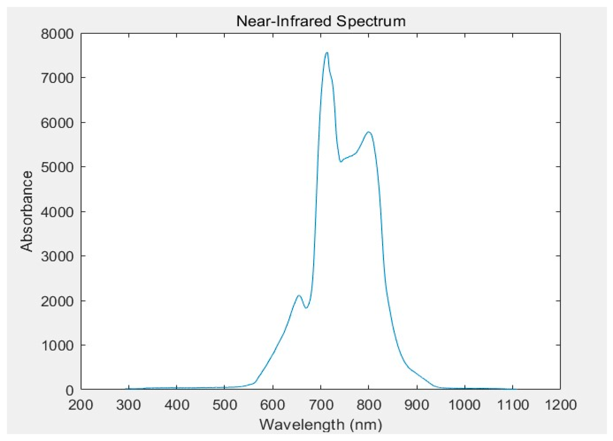
Figure 2.
Spectral pattern of stale citrus.
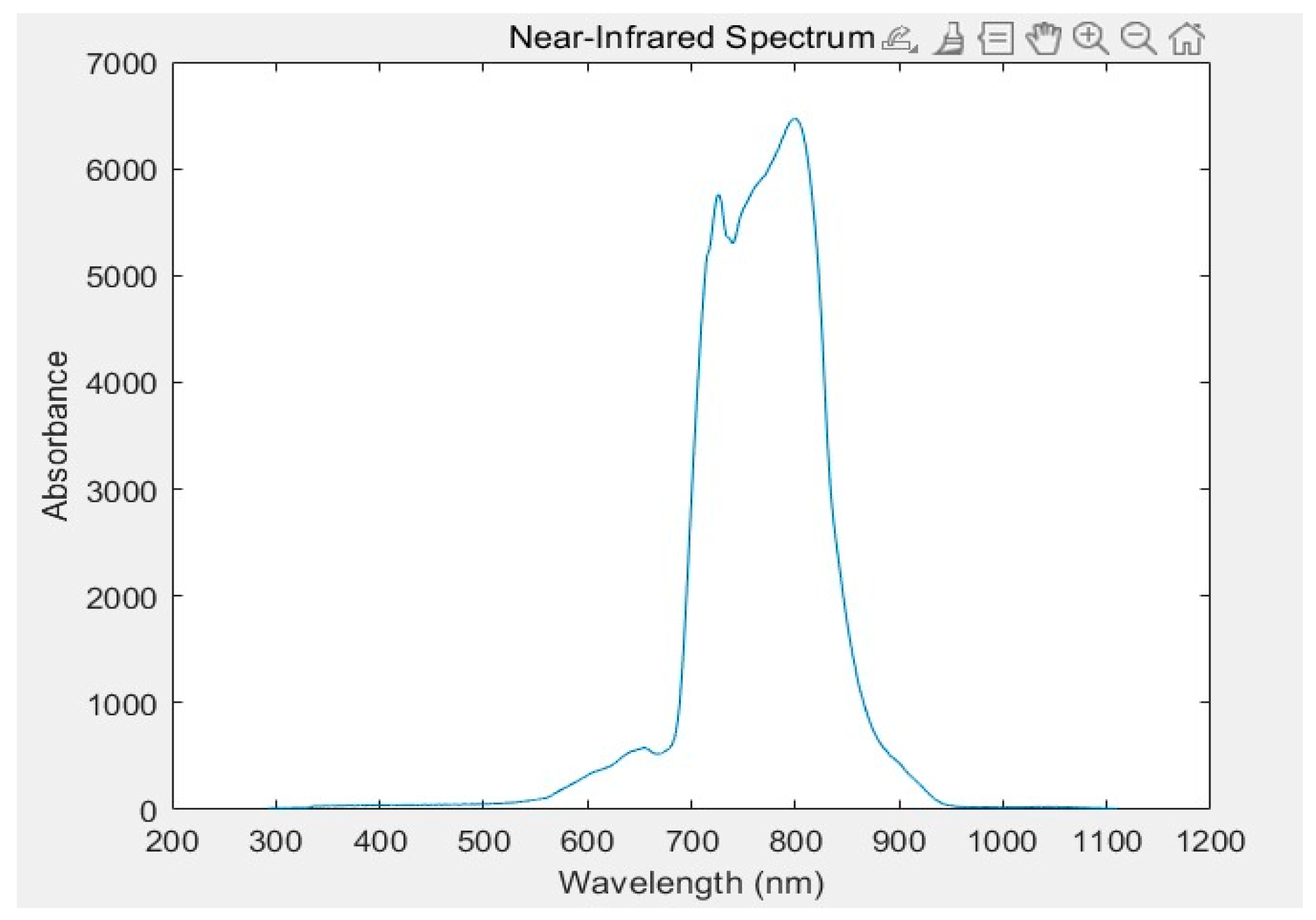
Figure 3.
Diagram of the structure the neural network.
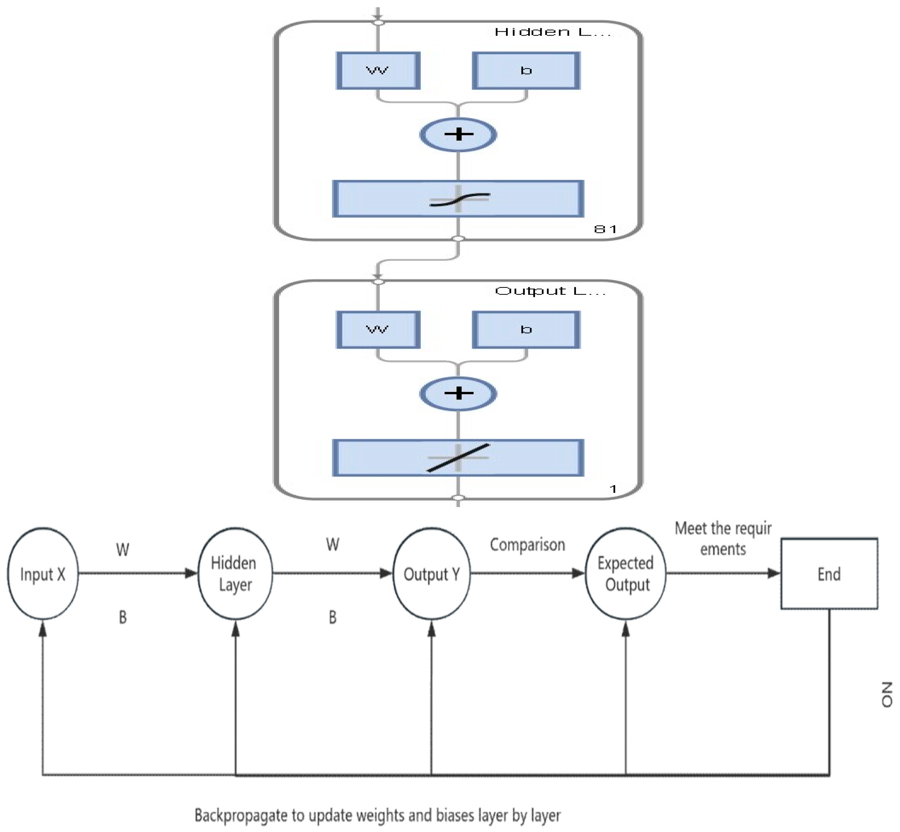
Figure 4.
Training indicators.
Disclaimer/Publisher’s Note: The statements, opinions and data contained in all publications are solely those of the individual author(s) and contributor(s) and not of MDPI and/or the editor(s). MDPI and/or the editor(s) disclaim responsibility for any injury to people or property resulting from any ideas, methods, instructions or products referred to in the content. |
© 2024 by the authors. Licensee MDPI, Basel, Switzerland. This article is an open access article distributed under the terms and conditions of the Creative Commons Attribution (CC BY) license (http://creativecommons.org/licenses/by/4.0/).
Copyright: This open access article is published under a Creative Commons CC BY 4.0 license, which permit the free download, distribution, and reuse, provided that the author and preprint are cited in any reuse.


