Submitted:
08 June 2024
Posted:
11 June 2024
You are already at the latest version
Abstract
Background: To rigorously derive easy to use formulae for the inclination angle for single cut rotation osteotomy that can be used for tibia deformity correction.
Method: Three theorems were proven using trigonometric identities and concepts of linear algebra. These were rigorously shown. The three concepts were how to convert deformities in an AP/Lateral plane to an oblique plane deformity with a true angular magnitude of deformity; how to project an angular quantity from one plane to another; and the calculation of the inclination angle for the oblique osteotomy plane. All figures in this article were created by the authors of this paper.
Results: From the formula derived, a statistical t-test was performed that showed no significant difference between the formula derived in this paper and the original Sangeorzan paper charts (p=0.0079).
Conclusions: The formulae described in this article are a method to accurately calculate the inclination angle of the osteotomy for a single cut rotational osteotomy for tibial deformity correction.
Clinical Relevance: The article gives a deeper understanding of fundamental concepts behind deformity correction and provides an easy-to-use mathematical formula to calculate the osteotomy inclination for single cut rotational osteotomies.
Keywords:
osteotomy
; deformity
; oblique
; rotation
; angulation
1. Introduction
A mathematically directed single-cut osteotomy for correction of tibial malunion was originally described by Bruce Sangeorzan and allows for correction of angular deformity along coronal, sagittal, and axial plane with a single oblique cut.4 The purpose of this article is to provide easy to use mathematical formulae to describe both the plane of the osteotomy and its inclination and demonstrate their derivation. The formula represents an exact solution to the problem.
- Methodology and Mathematical Proofs:
The method of demonstrating the osteotomy angle for the single cut osteotomy will have four parts. The first part will review how to calculate the magnitude of the true deformity and the plane that the deformity exists in. This is critical because the inclination angle lies in the ‘no deformity’ view on the x-ray which is orthogonal to the view that demonstrates the true deformity. The second part will go over a mathematical corollary needed to arrive at the formula shown in the third part which is the inclination angle. The final part will discuss sign convention and deciding whether to make it a descending or ascending cut.
- 1.
- Calculation of Magnitude of True Deformity and Plane of Deformity
- First, we must define out variables:
- P= Plane of deformity measured in degrees
- A= True magnitude of deformity measured in degrees measured in the plane of deformity
- AP=Magnitude of deformity in AP plane (what is measured on radiographs)
- LAT=Magnitude of deformity in Lateral Plane (what is measured on radiographs)
The computation of finding the plane of the deformity and the true magnitude of deformity has been described on many accounts. Paley demonstrated a proof of this in his book.3 The computation is similar to converting rectangular coordinates into spherical coordinates on a 3-dimentional grid. Refer to Figure 1 to follow the proof below.
□
Figure 1.
Finding the plane of a deformity along with its true magnitude.

- 2.
- Corollary Theorem of Angular Projections
The next theorem is necessary to computing the angle of the osteotomy for both angular and rotational correction. The question is – suppose there is an angle X1 on a Plane 1 and there is a second plane (plane 2) that intersects Plane 1 at angle G. If we were to project the angle X1 from plane 1 onto plane 2 – what will the new angle be on Plane 2. We will call this angle X2.
Refer to Figure 2 for this proof. Again, we begin by defining our variables:
- Plane 1 and Plane 2 are two planes that intersect each other at an Angle G
- Angle G= Angle between both planes
- X1= Angle on Plane 1
- X2= Angle projected from plane 1 to plane 2
Figure 2.
Projection of an angle from one plane onto another intersecting plane.
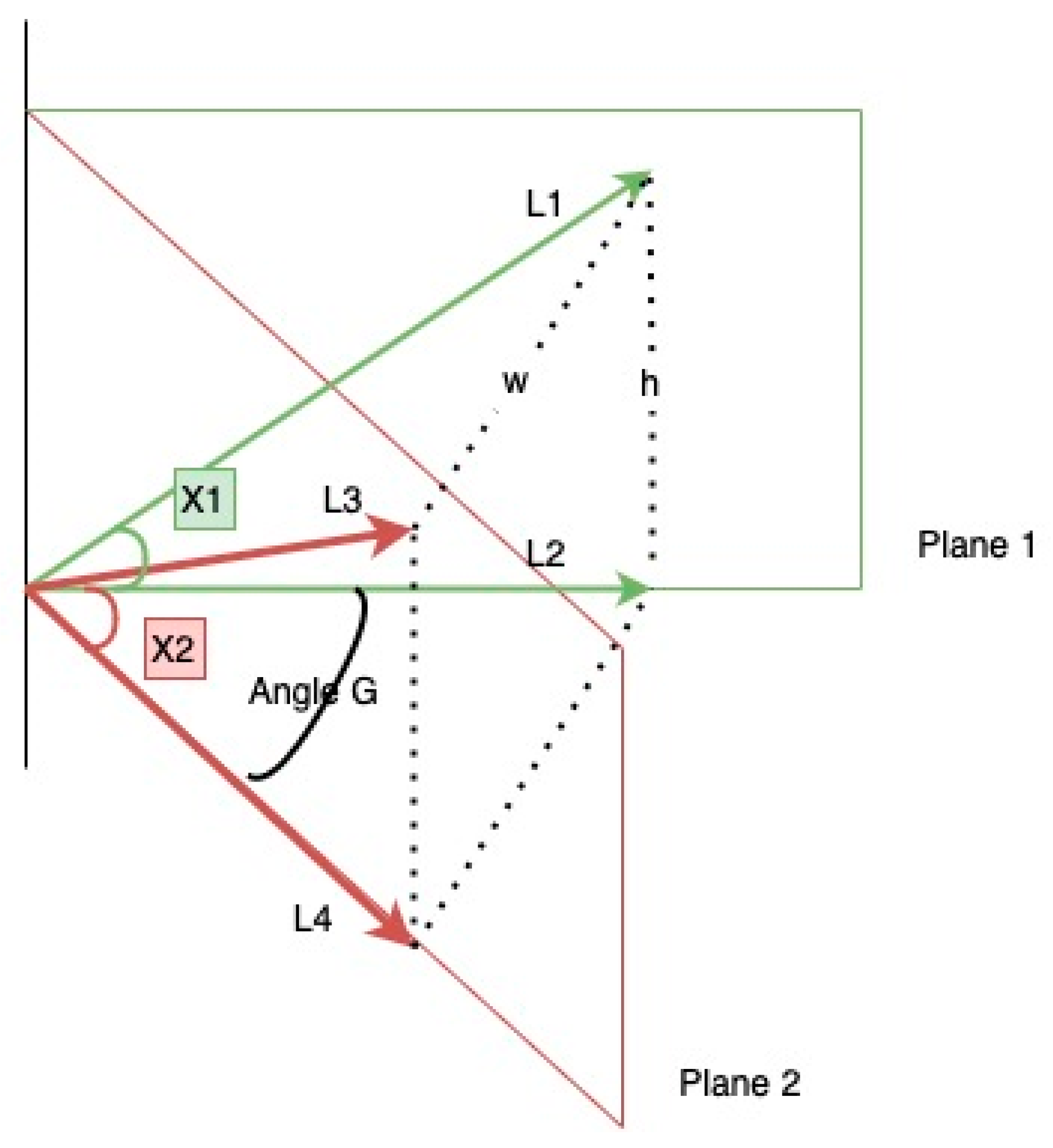
From the figure drawn out, you can derive the following from trigonometric relationships:
Solving this series of equations, you get:
□
This relationship is noteworthy for the third part of this paper. In effect, it describes the relationship of an angle in one plane and the new angle formed in a new plane.
- 3.
- Calculation of Osteotomy Angle
Putting this all together, we can calculate the obliquity of the osteotomy angle. It is noteworthy that this obliquity is measured in the view where the bone appears most ‘straight.’ This is orthogonal to the plane of the maximal deformity (see Figure 3 and Figure 4). Again, we begin by redefining our variables, referring to Figure 5 for visual representation:
- P= Plane of Oblique-Plane Deformity
- A= Magnitude of Deformity
- R= Magnitude of Rotational Deformity
- B= Angle of Cut on the bone Relative to Line Orthogonal to Axis of Tibia in the plane orthogonal to the Plane of Deformity
- K=Rotation about the osteotomy plane. Represented in Figure 6.
Figure 6.
This demonstrates the angle K along the osteotomy plane.
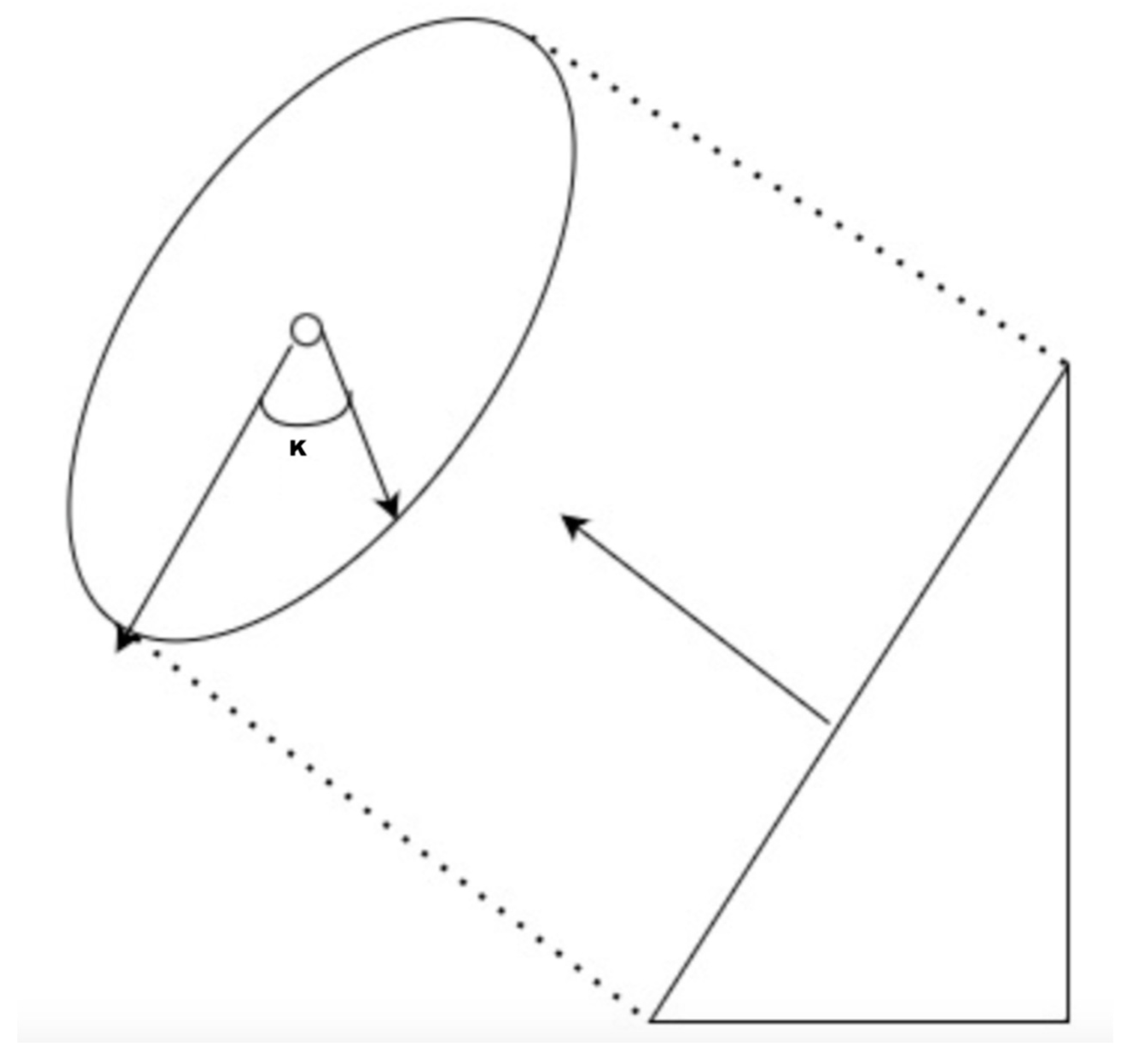
Recall earlier we derived the relationship of how one angle projects onto another intersecting plane as being:
If we use this corollary to project the axial view onto our oblique osteotomy at angle B - we can find the magnitude of angle K along the osteotomy plane
We can do the same by projecting the angular deformity onto the osteotomy plane:
By trigonometric identities, this equation can reduce to:
The value of K in both equations is equal. We can use that to rearrange the two equations above to obtain this relationship:
Further Rearrangement will yield the magnitude of B:
- 4.
- A Note on Sign Convention:
This concept is critical to understand because while the above formulae are adept at describing the magnitude of the osteotomy angle, the next question is whether the osteotomy is ascending versus descending. Performing a descending osteotomy when an ascending one is indicated will worsen the rotational deformity.
There are two ways to go about this. One is to adopt a consistent sign convention when performing calculations. The example would be akin to using the right-hand rule to determine what is positive and negative and referencing that with a x-y-z coordinate plate. This is difficult and can get confusing because the laterality (right versus left) makes it so that internal or external rotation on one side has the opposite sign convention on the other.
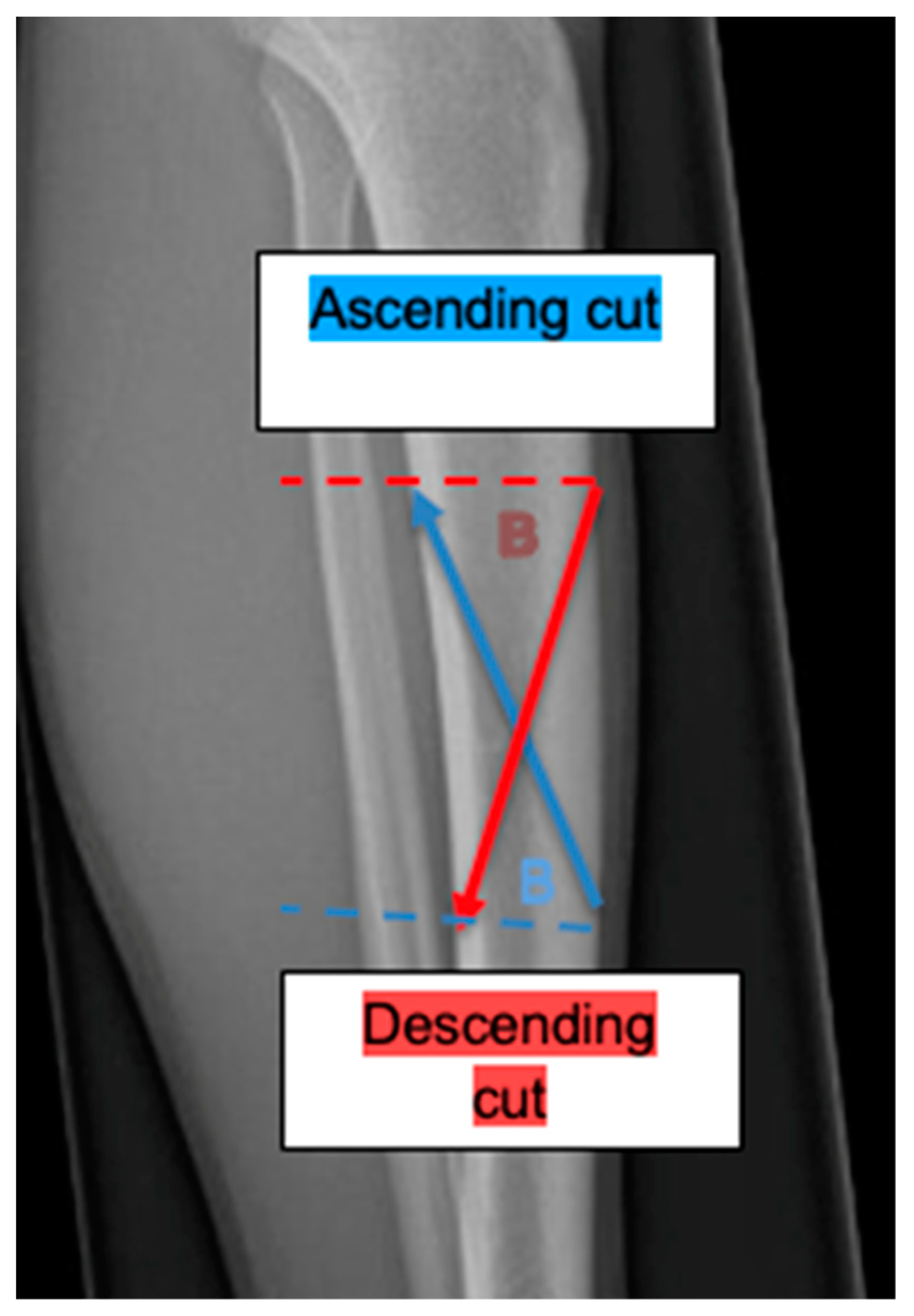
To simplify this – one can generalize these findings based on the laterality and the rotational deformity and the right-hand rule.2 The right-hand rule is a method to make the results consistent. One curls their fingers in the direction of the rotational deformity and the thumb points to the direction of the axis of the rotation. For an example, Applying the right-hand rule for a right limb with an internal tibial torsional deformity would have one’s thumb pointing superiorly. This indicates that the axis of rotation points superiorly. This would imply that the axis of rotation begins from posterior inferior and proceeds to anterior superior. A cut orthogonal to this would be ascending. A table utilizing this principle is illustrated in Table 1. Figure 7 demonstrates what is meant by an ascending cut and a descending cut and demonstrates how the angle B is defined relative to these cuts on a no deformity view x-ray.

| Laterality (Right vs Left) | Rotational Deformity | Osteotomy Inclination |
|---|---|---|
| Right | Internal Rotation | Ascending |
| Right | External Rotation | Descending |
| Left | Internal Rotation | Descending |
| Left | External Rotation | Ascending |
- Results – Verification Utilizing the Sangeorzan Charts
Given the conclusions above, we decided to validate our using the original paper by Sangeorzan. Table 2 is a chart that demonstrates a comparison between finding the inclination angle of the osteotomy using the formula described above and with the charts in Sangerozan’s article.
A statistical t-test was performed that showed no significant difference between the two methods (p=0.0079).
5. Discussion
Using trigonometric relationships, we were able to derive an exact solution as to the plane of the osteotomy. Additionally, in demonstrating the mathematical proofs rigorously, on can understand better how to implement these equations and limitations they pose. The final equations and variables are as follows:
- P= Plane of Oblique-Plane Deformity
- A= Magnitude of Deformity
- R= Magnitude of Rotational Deformity
- B= Angle of Cut on the bone Relative to Line Orthogonal to Axis of Tibia in the plane orthogonal to the the Plane of Deformity
- AP=Magnitude of deformity in AP plane
- LAT=Magnitude of deformity in Lateral Plane
It is noteworthy that the formula for P and B are incredibly similar. There is an elegant mathematical intuition to this. P represents the angle that is formed from the oblique plane from one of our rectangular coordinates. B on the other hand represents the oblique plane of the osteotomy that best projects the rotational deformity and angular deformity on it. Both represent very similar projections and the math demonstrates that elegantly. It stands to reason that the quantity K described above is the equivalent in some way to the ‘true magnitude’ of angulation and rotation combined.
These formulae were compared with the charts from the original Sangeorzan paper and found to correlate closely. The proof above serves to give insight into how to analyze deformity as well. In the face of a tibial deformity that has an angular component in an oblique plane with a torsional deformity as well, the recommended sequence is as follows:
- Orthogonal AP and Lateral films must be taken and the magnitude in each plane must be quantified accurately.
- Measurement of rotational deformity can be measured clinically, or more accurately through the use of CT.1
- Measurement of leg length inequality and translational deformity should also be undertaken as this may limit use of this method.
- Once angular and rotational deformities are measured, one must find the oblique plane of maximal deformity. Orthogonal to this plane is the “no deformity plane.” One can also compute the magnitude of this deformity.
- Once the magnitude of angular deformity is computed, one can compute the inclination angle.
- Use the table referenced above to determine whether the osteotomy is descending or ascending.
- In the operating room, begin the osteotomy by finding the XR view that shows ‘no deformity.’ Along this view is where the osteotomy is going to be made.
- Place a k-wire at the starting point of the osteotomy at the center of the deformity on this view for reference. Make sure the inserted k-wire is truly orthogonal to the “no deformity” view radiographically
- Using a sterile radio-opaque goniometer, place 2 more k-wires measured angle B from a line orthogonal to the axis of the bone on the no deformity view. Then the bone can be cut along these K-wires.
- Rotate the bone into its corrected position and provisionally fix. Confirm correction on AP-Lat Plane and clinically assess rotation of the limb. Fix the osteotomy definitively with standard internal fixation techniques.
To apply the mathematical principles above, one must be familiar with their limitations. This method does not address translational deformities in the coronal or sagittal plane. There may be some ‘lengthening’ that is due to correction of the angular deformity and not a true lengthening of the bone. One must understand that the mathematical implications do not reliably achieve lengthening or shortening of the deformed limb; however, the correction of the deformity is powerful and can correct coronal, sagittal, and axial plane deformity.
Finally, soft tissue considerations must always be taken into account. Neurovascular structures on the concavity of the deformity may be put under stretch in extreme deformities which may necessitate a different approach or possible gradual correction. The overlying soft tissue envelope must be able to accommodate a relatively large dissection, internal fixation, and must be mobile enough to move with the deformity which is not always the case in post-traumatic deformities.
References
- Jacob RP, Haertel M, Stussi E. Tibial torsion calculated by computerized tomograpy and compared to other methods of measurements. J Bone Joint Surg 1980; 62B:238-42.
- Paccola, C. A simplified way of determining the direction of a single-cut osteotomy to correct combined rotational and angular deformities of long bones. Rev. Bras. Orthop. 2010, 46, 329–334. [CrossRef]
- Paley, D. Oblique Plane Deformities. Principles of deformity correction. Springer. Baltimore MD. 193-194.
- Sangeorzan, B.J.; Sangerozan, B.P; Hansen, S.T.; Judd, R.P. Mathematically directed single-cut osteotomy for correction of tibial malunion. J. Orthop. Trauma 1989, 3, 267-275. [CrossRef]
Figure 3.
The view on the left demonstrates the view that would show the true deformity of the bone. Orthogonal to the is the view on the right that would show a straight bone (also known as the “No Deformity View.” The inclination of the osteotomy is measured on the view on the right.
Figure 3.
The view on the left demonstrates the view that would show the true deformity of the bone. Orthogonal to the is the view on the right that would show a straight bone (also known as the “No Deformity View.” The inclination of the osteotomy is measured on the view on the right.
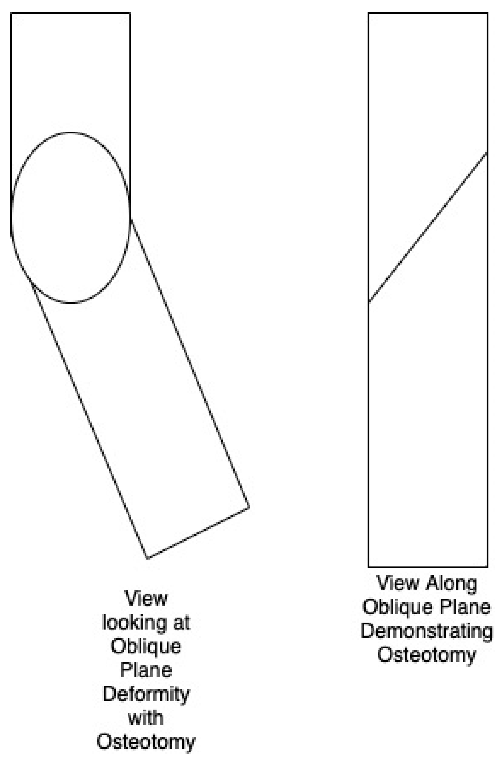
Figure 4.
This figure demonstrates the osteotomy in multiple orientations. The view on the very right is the no deformity view that we measure our osteotomy angle from.
Figure 4.
This figure demonstrates the osteotomy in multiple orientations. The view on the very right is the no deformity view that we measure our osteotomy angle from.
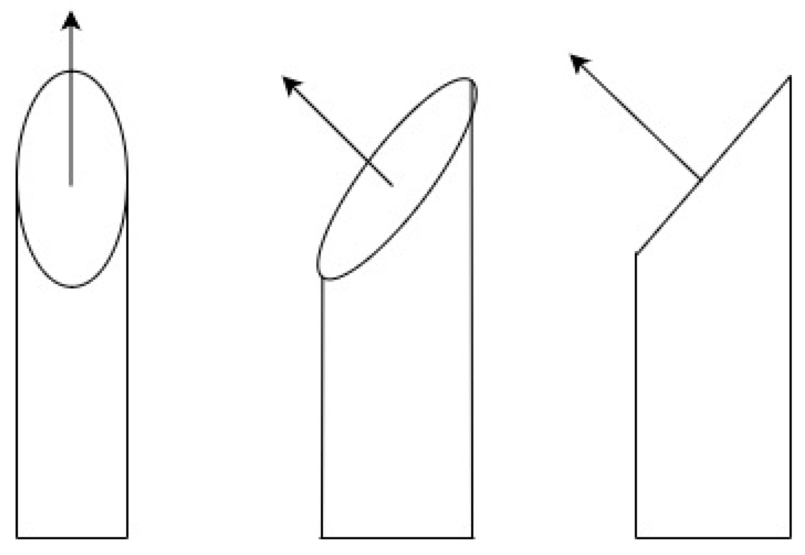
Figure 5.
Projections of rotational and angular deformities onto oblique osteotomy plane angled B degrees from a plane orthogonal to the axis of the bone from the view that does not show the boney deformity.
Figure 5.
Projections of rotational and angular deformities onto oblique osteotomy plane angled B degrees from a plane orthogonal to the axis of the bone from the view that does not show the boney deformity.
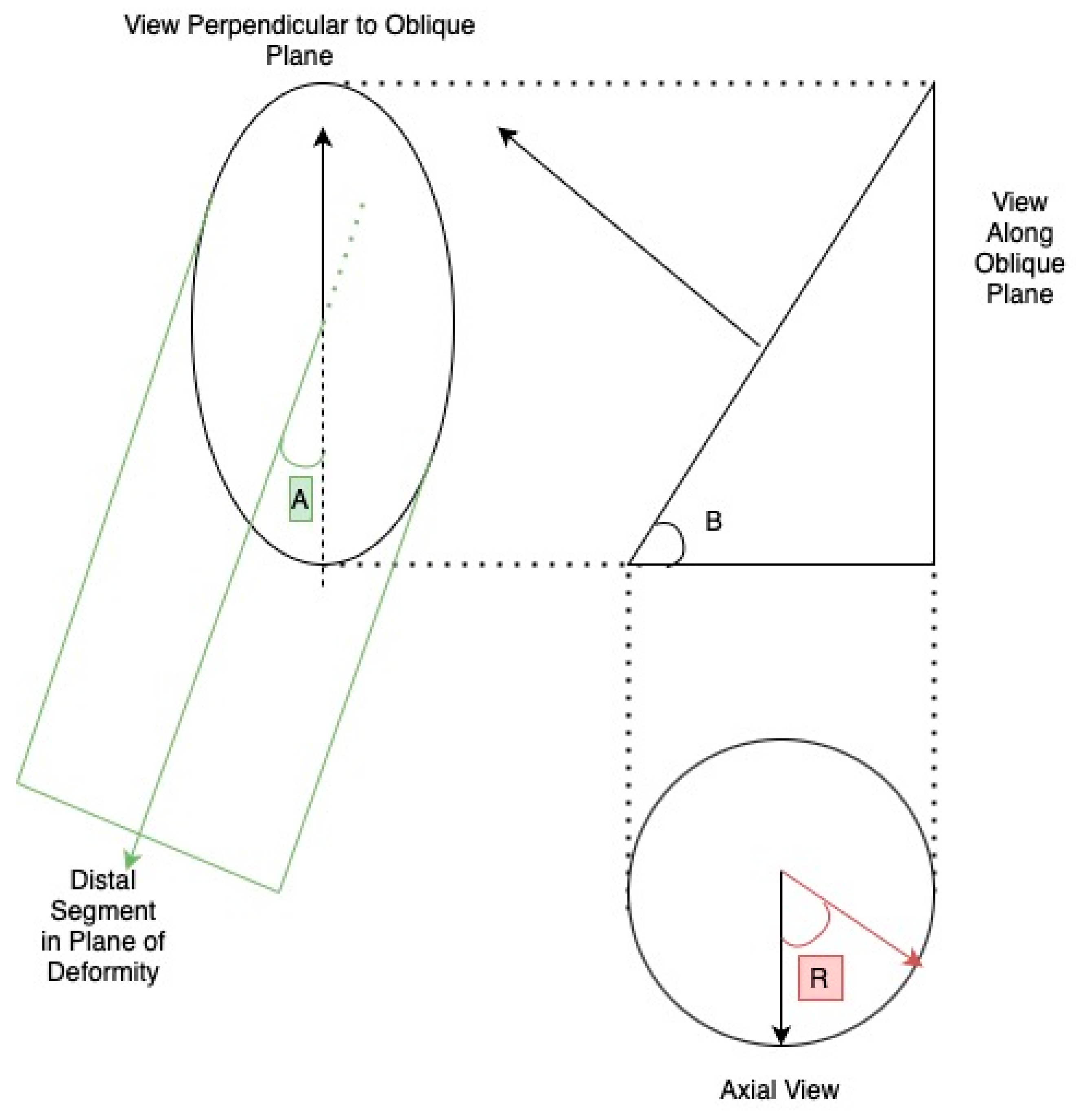
Figure 7.
This figure demonstrates what a descending cut (in red) and Ascending cut (blue) are. The angle B is demonstrated on each line to represent the magnitude of this angle. This X-Ray must be taken in the view orthogonal to the plane that demonstrates the true angulation of the deformity, also known as the “no deformity view.”.
| Angular Deformity (A) –degrees | Rotational Deformity (R) –degrees | Inclination Angle (B) Qatu et al Formula – degrees | Inclination Angle (B) Sangeorzan Chart –degrees |
| 5 | 5 | 45.0 | 45.0 |
| 10 | 5 | 63.6 | 60.0 |
| 15 | 5 | 71.9 | 70.0 |
| 20 | 5 | 76.5 | 75.0 |
| 5 | 10 | 26.3 | 25.0 |
| 10 | 10 | 45.0 | 45.0 |
| 15 | 10 | 56.7 | 55.0 |
| 20 | 10 | 65.2 | 63.0 |
| 5 | 15 | 18.1 | 17.0 |
| 10 | 15 | 33.3 | 31.0 |
| 15 | 15 | 45.0 | 45.0 |
| 20 | 15 | 53.6 | 52.0 |
| 5 | 20 | 13.5 | 15.0 |
| 10 | 20 | 25.8 | 25.0 |
| 15 | 20 | 36.4 | 37.0 |
| 20 | 20 | 45.0 | 45.0 |
Disclaimer/Publisher’s Note: The statements, opinions and data contained in all publications are solely those of the individual author(s) and contributor(s) and not of MDPI and/or the editor(s). MDPI and/or the editor(s) disclaim responsibility for any injury to people or property resulting from any ideas, methods, instructions or products referred to in the content. |
© 2024 by the authors. Licensee MDPI, Basel, Switzerland. This article is an open access article distributed under the terms and conditions of the Creative Commons Attribution (CC BY) license (http://creativecommons.org/licenses/by/4.0/).
Copyright: This open access article is published under a Creative Commons CC BY 4.0 license, which permit the free download, distribution, and reuse, provided that the author and preprint are cited in any reuse.


