Submitted:
11 June 2024
Posted:
11 June 2024
You are already at the latest version
Abstract
In this paper, we investigate the so-called electronic dressed states, a unified quasiparticle resulting from the interaction between electrons in a two-dimensional material with an off-resonance optical dressing field. If the frequency of this field is much larger than all characteristic energies in the system, such as the Fermi energy or bandgap(s), the electronic band structure is affected by radiation so that some important properties of the electron dispersions could be modified in a way desirable for practical applications. For example, a circularly polarized light can be used to vary the bandgap of Dirac materials: it opens a gap in graphene and other metallic and semimetallic lattices, or modifies the magnitude of an existing gap. This will either enhance or reduce a gap, depending on its initial value as well as properties of a host material. Here, we consider gaped dice and Lieb lattices as samples, and put forward a full theoretical model to reveal how these electronic states are deformed by an elliptically-polarized irradiation with a focus on generation and modification of a bandgap.
Keywords:
two-dimensional materials
; alpha-T3 model
; graphene
; dice lattice
; electron-photon interaction
; dressed states
; off-resonance dressing field
; electronic and optical properties of low-dimensional lattices
1. Introduction
Floquet theory, which was originally developed to solve partial differential equations, [1] represents a unique tool for describing the electronic properties and behavior of a large number of diverse quantum systems in the presence of high-frequency periodic dressing fields. [2,3,4,5] It has also advanced into the so-called Floquet engineering, a technique for obtaining the electronic dispersions and, specifically, bandgaps which are required for technical applications. This has quickly become one of the most promising research directions in condensed matter physics and photonics. [6,7,8,9,10] The Floquet engineering is primarily applied to two-dimensional (2D materials, or the surface states of three-dimensional (3D) lattices. Because of the recent experimental advances in laser and microwave optics, it has become possible to verify the theoretical predictions of condensed matter quantum optics in actual experiments and realize them in optoelectronic devices. [11]
Floquet theory has been successfully applied to original, [12,13,14,15,16,17] gapped [13,18] and Kekule-patterned graphene. [19] It also enters into extensive studies of anisotropic [20] and tilted Dirac materials [21,22,23,24,25,26,27] as well as other structures. [12,28,29,30,31,32]. A special interest was put on Floquet control of electronic transport properties of irradiated materials [33,34,35] in addition to indirect exchange interaction, [36,37] and collective behaviors. [38,39] Its interests further extend to the fields of excitonic [40] and dissipative [9] Floquet systems, pseudospin textures, and nanoribbons. [41,42,43,44,45] In particular, optical-dressing field was utilized to create localized trapped states, [46] similarly to those in fullerenes [47,48,49,50].
In fact, electron-photon interaction and their dressed states are only one part of an ongoing effort to investigate all electronic and collective properties in recently discovered Dirac materials. These efforts include establishing a Wentzel-Kramers-Brillouin (WKB) theory for taking into consideration of semi-classical electronic states in -, dice and even Kekule-patterned graphene [51,52], in a way very similar to previously reported successive works on genuine graphene materials [53,54,55].
Moreover, Floquet engineering is utilized to alter the Bloch-electron states in Dirac materials with a flat band, such as a dice lattice. [7,56,57] The - model, which represents interpolation between a graphene and a dice lattice, becomes one of the most favorable and well-studied models for materials acquiring a flat band. A strong and ongoing interest on this - model is attributed to its unusual low-energy electronic band structure involving a regular graphene Dirac cone as well as a flat band. This actually makes - materials as a candidate for replacing graphene in modern electronic devices.
The atomic structure of the - materials consists of an additional atom at the center of a graphene-like honeycomb lattice (HCL). Therefore, the new hub-to-rim (and rim-to-hub) hopping coefficient can be related to an existed rim-to-rim hopping simply by a scaling parameter , which turns out to be a key factor for characterizing various - materials. For example, the case with corresponds to a dice lattice, while resembles graphene with a fully decoupled set of hub atoms at the center of each hexagon. Importantly, electronic properties of - model can be described by a pseudospin-1 Dirac-Weyl Hamiltonian which directly depends on a parameter or, more specifically, on its phase .
The presence of an unusual band structure in - model can lead to unique and unexpected features, including electronic, [58,59,60] collective, [61,62,63] magnetic, [64] optical properties, [65,66,67,68,69] and even a phase transition [70]. These behaviors are very different from those of graphene. The major issue addressed by many researchers has focused on how these graphene-like properties will be modified by the presence of an additional flat band. [71,72,73] Already, a variety of materials, with their electronic properties described approximately by an - model, have already been identified and made by synthesis, and meanwhile, the presence of such a stable flat-band in their energy spectrum has been experimentally verified. Particularly, the so-called Lieb lattice, which has already been demonstrated in a number of different systems and wave-guides, [74,75,76] presents a new type of technologically-promising pseudospin-1 Hamiltonian, and its corresponding inverted band structure reveals a finite bandgap as well as a flat band which lies within this bandgap but intersects the upper (valence) band at its bottom. [77,78,79]
The remaining part of this paper is organized as follows. In Section 2, we review the electronic properties, including energy band structure, and electronic states of - materials, a dice lattice as well as a Lieb lattice. Specifically, we discuss the properties of an - model with a fixed finite bandgap induced by a dielectric substrate. Moreover, the electron-dressed states due to an applied off-resonance circularly and, more generally, elliptically polarized irradiation, including related derivations, equations, and mathematical formalism are all presented in Section 3. Section 4 is devoted to detailed discussion of our numerical results and their connections to the band structure of electronic dressed states associated with different materials. Our concluding remarks are made in the final Section 5.
2. Low-Energy Electronic States of the Considered Materials
The electronic states of the model are described by the following low-energy -dependent pseudospin-1 Hamiltonian
where depends on the valley index , is the two-dimensional wave vector, . Phase is related to the relative hopping parameter as , and the Fermi velocity denoted by must be exactly equal to that in graphene in order to enable a smooth transition between all the materials, including the limiting cases of graphene and a dice lattice .
Remarkably, Hamiltonian (1) could be presented in a generalized form
where vector depends on valley index and the -dependent matrices represent a generalization of regular Pauli matrices
and
Hamiltonian (2) represent a general -dependent model. For , matrices (3) and (4) are reduced to the standard Pauli matrices. Hamiltonian (1) or (2) also becomes equivalent to that of graphene. [80]
For the other limit, corresponding to a dice lattice with , expressions (3) and (4) accept a simplified and symmetric form of spin-1 Pauli matrices:
and
Consequently, the Hamiltonian in Equation (1) could be rewritten as a symmetric and compact form, i.e.
where .
The energy dispersions of an material, corresponding to Hamiltonian (1) are obtained as
where the three solutions (8) are related to the valence (), conduction () and flat () bands of the electronic structure. The energy dispersions (8) do not directly depend on and, therefore, are also the same for for a dice lattice.
The wave functions for the model, obtained as the eigenfunctions of Hamiltonian (1), are calculated as [57,69]
and
Unlike dispersions (8), wave functions (9) and (10) directly depend on phase and valley index .
For the case of a dice lattice, wave functions (9) and (10) are reduced to
and
Such a symmetric form of wave functions (11) and (12) have a strong effect on several crucial electronic properties, such as Klein tunneling.
2.1. The Model with a Finite Gap
Importantly, an material could also acquire a finite gap in a complete analogy to graphene. [81] It could be induced either by a special type of a dielectric substrate, or by a circularly polarized dressing field.
In particular, we are very interested to investigate how an existing bandgap in an lattice created by a substrate, would be modified or renationalized if a curricular polarized irradiation is also added. Therefore, we put a gapped model in the focus of our study.
The Hamiltonian of the gapped model is explicitly given as
where is the induced gap parameter.
Similarly to graphene, the Hamiltonian for the gapped model (13) is modified as
meaning that Hamiltonian (1) receives an additional term
which is explicitly given as
Here, the -dependent generalization of the remaining Pauli matrix .
We immediately discern that in the presence of a finite bandgap , the energy spectrum for flat band of an material with undergoes a special type of a deformation which results in a finite k-dispersion, i.e., the flat band is no longer flat. Finding the complete energy dispersions for the gapped model is a challenging problem, which involves solving a cubic equation. [56,73] However, it is relatively straightforward to verify that Hamiltonian (13) results in two inequivalent gaps between the conduction and flat, and the flat and the valence bands which depend on parameter (or phase ) and valley index .
For a dice lattice with , it is simplified as
and Hamiltonian (13) is presented in the following form
In contrast to the Hamiltonian (1) for the general model, eigenvalue equation corresponding to Equation (18) results in a symmetric band structure with two equal bandgaps and a unaffected flat band right in the middle between the valence and conduction bands (see Figure 1). Therefore, the flat bans is deformed and received a finite k-dispersion for all materials with a finite gap, expect foe a dice lattice with .
2.2. Lieb Lattice
Flat bands have also been realized in some other types of lattices, mostly, optical Lieb and Kagome lattices. A Lieb lattice was observed in a number of existing systems and experimental setups: organic materials, optical lattices and waveguides
A Lieb lattice is made of three displaced square sublattices. The Hamiltonian of a Lieb lattice is
where
and is the lattice parameter.
The three energy dispersions, corresponding to Hamiltonian (19), are and which could be written using a single unified expression
where is Kronecker symbol. As a result, we have obtained three energy subbands. One of them is a flat band, while the other two have a finite dispersion, such as shown in Figure 2. In a Lieb lattice the flat band is located at the finite energy right next to the lowest point of the conduction band, while for the case of a dice lattice with a finite gap, it is located symmetrically between the valence and conduction bands.
The corresponding wave functions are given by
and
for the flat band.
3. Electron Dressed States: General Formalism
Let us now consider the changes in the energy dispersions of gapped when an off-resonance high-frequency irradiation is applied. It is known that the results of such irradiation drastically depend on its polarization type: circularly polarized light modifies the existing energy bandgap, while the linearly polarized field indueces an anisotropy of the electron energy dispersions in the direction of the light polarization.
We will consider the most general case of elliptically-polarized dressing field. If the direction of the light polarization is aligned with the x-axis, its vector potential is given as
where is the electric field of the imposed irradiation, so that its intensity is , and is its frequency meaning that for the high-frequency regime coefficient represents only a small correction.
Parameter is the ratio of field strengths (electric field amplitudes) along the two axes of the polarization ellipse. Equation (24) corresponds to the most general type of the light polarization. Thus, where results in a known expression
for the circularly polarized light, while a limit of corresponds to the dressing light of a linear polarization
Thus, considering the general elliptical polarization of the imposed irradiation allows us immediately discern the results for these crucial situations as well.
It is well-known that the energy dispersions of the electron dresses states due to an off-resonant dressing field are obtained by applying the canonical substitution
in the Hamiltonian (1), which corresponds to a non-irradiated material.
As a result, Equation (1)
receives an additional interaction Hamiltonian term
where
which would correspond to circularly-polarized light. Parameter , which specifies the strength of the interaction between an electron and a photon, and has a unit of energy. This interaction strength parameter is the same for the irradiation with different types of polarization, meaning that an irradiation of specfic intensity and frequency effects the electronic band structure of graphene (or and material) at the same level, disregarding of its polarization. The way how the dispersions are affected, is obviously very different for the different types of polarizations. For our future calculations, we will also need another type of coupling parameter , which is now dimensionless in contrast to the previously considered . For the considered off-resonance regime, we can assume , which will be later used as a series expansion parameter.
The key idea for using the Floquet-Magnus perturbation approach is as follows. First, we rewrite the interaction Hamiltonian term in the form of two time-independent complimentary conjugate terms
where +H.c. means Hermitian conjugate. Operator and its Hermitian conjugate are time-independent.
Comparing Hamiltonian (29) and representation (31), we can immediately derive the explicit form of the perturbation operator as
Once this is done, the effective time-independent Hamiltonian representing our dressed-state system is presented as
where is a commutator.
Since in our consideration of the off-resonance regime , it is sufficient to take into consideration only the first few terms of expansion (33).
Matrix (32) is not Hermitian for any , which is true for any type of the light polarization excpept the linear one, including the cicrularly polarized irradiation with . However, it is purely real for all types of Dirac material with chiral terms in Hamiltonian (1), for both zero or finite bandgap .
The zero-order term in expansion (33) must be equivalent to Hamiltonian (1) of an material in the absence of the dressing field. The next term is evaluated as
whose structure is equivalent to that of the bandgap term (16).
This unexpected result reveals a lot of interesting features of the electron dressed states for the circular and elliptical polarizations of the dressing field. Most importantly, we know that term (34) mainly determines the bandgap of the radiated materials since it doesn’t depend on wave vector components and . It represents the key contribution for the energy dispersions at since the next term would only result in a much smaller correction. Therefore, we find that for the linearly polarized light with , the band gap remains completely unaffected by the dressing field.
The gap due to the circular polarized light is formed pretty much the same way as the initial bandgap , which is induced by a specific substrate. However, there is a very important difference: the irradiation-induced bandgap (34) is proportional to the valley index . Therefore, the total gap of the irradiated materials could be either increase or decreased, depending on whether we are considering the electronic states in the K or - valley ().
After evaluating the commutation relation in Equation (33), we arrive at the following expression for the effective perturbation Hamiltonian up to the order of
where
and, finally,
which would vanish for a circularly polarized light , as well as for graphene and a dice lattice .
3.1. Dressed States for a Lieb Lattice
Comparing Hamiltonian (19) and representation (31), we can immediately derive the explicit form of the perturbation operator as
The second-order correction for a Lieb lattice is calculated in the following way
Similarly to the previously considered model, term (45) represents correction which is small in the off-resonance regime .
4. Results and Discussion
Our main goal is to investigate the band structure of the electron dressed states for the materials with a finite gap. i.e., to understand how the existing gaps are modified or renormalized due to the elliptically polarized dressing field.
First, we find that according to equation (34), which demonstrates how in principle the band Gap is created for , the structure of the gap induced by the dressing field is pretty much similar to the existing gap given by equation (13). However, an important difference between the two types of the gap is that the irradiation-induced gap directly depends on the valley index , and is opposite for the K and K’ valleys. Therefore, the result for the two valleys is exactly the opposite, and the same initial gap could be either decreased or increased depending on the value of . This is exactly what we see comparing the upper and the lower panels of Figure 3, Figure 4 and Figure 5.
In our calculations, the following system of units is employed. All the energy values, including bandgap , are measured in terms of a typical graphene Fermi energy , which is obtained as . Here, is the corresponding Fermi momentum, which is also a reciprocal to our unit of length , and denote the areal electron doping density and the Fermi velocity and, respectively. Thus, for a typical density , we obtain , and .
Our numerical results shown in Figure 3 demonstrate how a finite bandgap is opened for initially gapless materials, as it is always expected due to the circularly polarized dressing field. In contrast, the change of the existing bandgap presented in Figure 4, substantially depends on the electron-light coupling constant , initial bandgap , phase , and valley index . We see that the bandgaps and the dispersions of the dress state subbands could be modified in completely different ways, depending on the material parameters of a specific lattice.
Importantly, we also reveal a substantial dependence of the irradiation-induced bandgap on phase . For the specific situation demonstrated in Figure 5 with the initial bandgap , we see that both gaps are significantly increased for the larger values of , just like the equivalence (the differences) between the two gaps.
The dressing field of an elliptical polarization with (in contrast to the circularly polarized light with ) is expected to induce a finite anisotropy and an angular dependence of the initially isotropic dispersions with a circular constant-energy cut. This is exactly what we see in Figure 6. However, we also note that the obtained elliptical dispersions significantly depend on phase . Both the shape and the size of the constant-energy cut of the electron dressed state energy dispersions are changed a lot more significantly for larger values of or relative hopping parameter .
The way how the energy dispersions of the dressed states are formed in a Lieb lattice is drastically different from that for the gapped materials. First, we have much less parameters to consider here. The bandgap and the exact locations of the energy subbands of a non-irradiated lattice are fixed and the main question here is whether once the dressing field is imposed, the flat band would remain flat, like in a dice lattice, or receive a finite curvature, just as we observed for the general model with .
Our numerical results, presented in Figure 7 and Figure 8, clearly demonstrate that the flat band receives a finite dispersion and its convex-concave type of curvature does not remain the same. Therefore, for any finite coupling parameter , the subbands cannot be described by the parabolic dispersions obtained using a constant-mass approximation. Moreover, for a large , the former-flat band; ’s location is such that its energy could only decrease for the larger values of the wave vector k (see Figure 8 (f)).
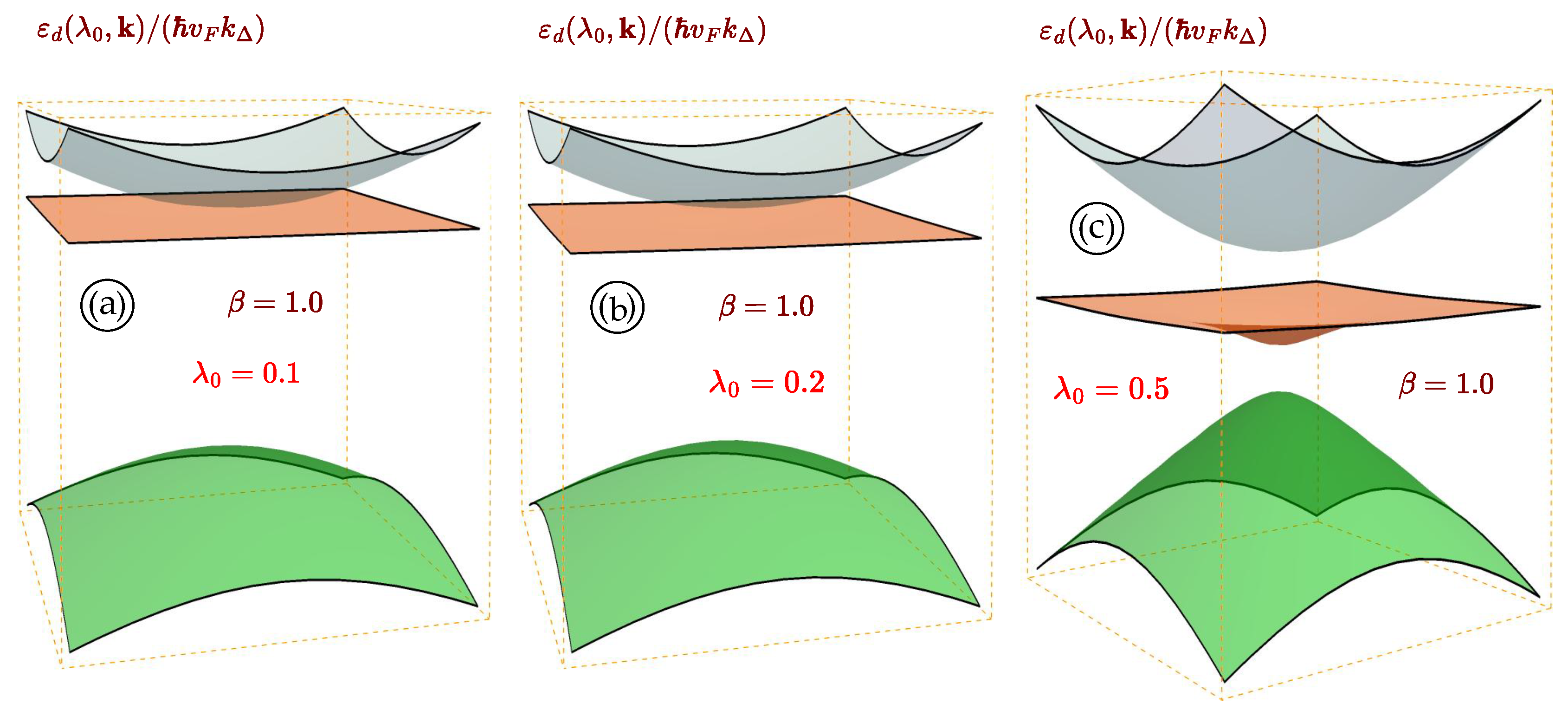
The degeneracy at is clearly lifted, and we observe three inequivalent bandgaps between the valence, flat, and conduction bands. The locations of the valence and conduction bands also change. Each of the two gaps is decreased, and the k-dependence becomes more significant. The situation becomes very different for a large , for which we find that all three subbands demonstrate low dispersions (reduced dependence on k), while each of the gaps is significantly modified.
5. Summary and Remarks
In this paper, we have performed a rigorous theoretical and numerical investigation into the electron-photon interactions and the resulting electron dressed states for some specific types of Dirac cone materials whose low energy spectrum exhibits a flat band and a finite bandgap.
If an electron in a two-dimensional material is irradiated with a high-frequency off-resonance dressing field, its interaction with the irradiation results in a specific unified quantum state with modified energy dispersions and bandgaps. The properties of the obtained dressed states strongly depend on the type of polarization of the imposed radiation. While a linearly polarized dressing field is known to induce finite anisotropy, circularly polarized light is known as a tool to open or modify the existing energy gap.
Our main goal was to consider the modification or renormalization of the existing band gaps of pseudospin-1 Dirac cone materials with a flat band. Specifically, we focus on the gapped model, a dice lattice, and a Lieb lattice. Each of these materials has a very distinguished energy band structure, but their common feature is the existence of a dispersionless flat band, as well as finite gaps between the valence, flat, and conduction bands.
In particular, our work contains a theoretical and numerical study of the dressed states in these materials, which includes the derivation of several crucial analytical relations for the energy dispersions in the presence of circularly and elliptically polarized light. We have demonstrated that the existing bandgap could be either increased or decreased depending on several material parameters of the specific lattice and the valley index. We have shown that for the and the Lieb lattice, the flat band received finite dispersions and a k-dependence, the valence and conduction bands and the corresponding bandgaps between them are also modified due to the dressing field.
References
- Kuchment, P.A. Floquet theory for partial differential equations; Vol. 60, Springer Science & Business Media, 1993. [CrossRef]
- Goldman, N.; Dalibard, J. Periodically driven quantum systems: effective Hamiltonians and engineered gauge fields. Physical review X 2014, 4, 031027.
- Eckardt, A.; Anisimovas, E. High-frequency approximation for periodically driven quantum systems from a Floquet-space perspective. New Journal of Physics 2015, 17, 093039. [CrossRef]
- Oka, T.; Kitamura, S. Floquet engineering of quantum materials. arXiv preprint arXiv:1804.03212 2018. 10.1146/annurev-conmatphys-031218-013423.
- Castro, A.; De Giovannini, U.; Sato, S.A.; Hübener, H.; Rubio, A. Floquet engineering the band structure of materials with optimal control theory. arXiv preprint arXiv:2203.03387 2022. [CrossRef]
- Cheng, Q.; Pan, Y.; Wang, H.; Zhang, C.; Yu, D.; Gover, A.; Zhang, H.; Li, T.; Zhou, L.; Zhu, S. Observation of anomalous π modes in photonic Floquet engineering. Physical review letters 2019, 122, 173901. [CrossRef]
- Weitenberg, C.; Simonet, J. Tailoring quantum gases by Floquet engineering. Nature Physics 2021, 17, 1342–1348. [CrossRef]
- Wang, B.; Ünal, F.N.; Eckardt, A. Floquet engineering of optical solenoids and quantized charge pumping along tailored paths in two-dimensional Chern insulators. Physical Review Letters 2018, 120, 243602. [CrossRef]
- Dehghani, H.; Oka, T.; Mitra, A. Dissipative Floquet topological systems. Physical Review B 2014, 90, 195429. [CrossRef]
- Nakagawa, M.; Slager, R.J.; Higashikawa, S.; Oka, T. Wannier representation of Floquet topological states. Physical Review B 2020, 101, 075108. [CrossRef]
- Koutserimpas, T.T.; Fleury, R. Nonreciprocal gain in non-Hermitian time-Floquet systems. Physical review letters 2018, 120, 087401. [CrossRef]
- Kibis, O.; Boev, M.; Kovalev, V.; Shelykh, I. Floquet engineering of the Luttinger Hamiltonian. Physical Review B 2020, 102, 035301. [CrossRef]
- Kibis, O.; Dini, K.; Iorsh, I.; Shelykh, I. Floquet engineering of gapped 2D materials. Semiconductors 2018, 52, 523–525. [CrossRef]
- Kibis, O. Metal-insulator transition in graphene induced by circularly polarized photons. Physical Review B 2010, 81, 165433. [CrossRef]
- Iurov, A.; Gumbs, G.; Roslyak, O.; Huang, D. Anomalous photon-assisted tunneling in graphene. Journal of Physics: Condensed Matter 2011, 24, 015303. [CrossRef]
- Perez-Piskunow, P.M.; Usaj, G.; Balseiro, C.A.; Torres, L.F. Floquet chiral edge states in graphene. Physical Review B 2014, 89, 121401. [CrossRef]
- Calvo, H.L.; Pastawski, H.M.; Roche, S.; Torres, L.E.F. Tuning laser-induced band gaps in graphene. Applied Physics Letters 2011, 98, 232103. [CrossRef]
- Kibis, O.; Dini, K.; Iorsh, I.; Shelykh, I. All-optical band engineering of gapped Dirac materials. Physical Review B 2017, 95, 125401. [CrossRef]
- Mojarro, M.; Ibarra-Sierra, V.; Sandoval-Santana, J.; Carrillo-Bastos, R.; Naumis, G.G. Dynamical Floquet spectrum of Kekulé-distorted graphene under normal incidence of electromagnetic radiation. Physical Review B 2020, 102, 165301. [CrossRef]
- Iurov, A.; Zhemchuzhna, L.; Gumbs, G.; Huang, D. Exploring interacting Floquet states in black phosphorus: Anisotropy and bandgap laser tuning. Journal of Applied Physics 2017, 122, 124301. [CrossRef]
- Gomes, Y.; Ramos, R.O. Tilted Dirac cone effects and chiral symmetry breaking in a planar four-fermion model. Physical Review B 2021, 104, 245111. [CrossRef]
- Iurov, A.; Zhemchuzhna, L.; Gumbs, G.; Huang, D.; Tse, W.K.; Blaise, K.; Ejiogu, C. Floquet engineering of tilted and gapped Dirac bandstructure in 1T’-MoS 2. Scientific Reports 2022, 12, 21348. [CrossRef]
- Mojarro, M.; Carrillo-Bastos, R.; Maytorena, J.A. Optical properties of massive anisotropic tilted Dirac systems. Physical Review B 2021, 103, 165415. [CrossRef]
- Sandoval-Santana, J.; Ibarra-Sierra, V.; Kunold, A.; Naumis, G.G. Floquet spectrum for anisotropic and tilted Dirac materials under linearly polarized light at all field intensities. Journal of Applied Physics 2020, 127, 234301. [CrossRef]
- Mehmood, F.; Pachter, R.; Back, T.C.; Boeckl, J.J.; Busch, R.T.; Stevenson, P.R. Two-dimensional MoS 2 2H, 1T, and 1T’ crystalline phases with incorporated adatoms: theoretical investigation of electronic and optical properties. Applied Optics 2021, 60, G232–G242. [CrossRef]
- Tan, C.Y.; Yan, C.X.; Zhao, Y.H.; Guo, H.; Chang, H.R.; et al. Anisotropic longitudinal optical conductivities of tilted Dirac bands in 1 T’- Mo S 2. Physical Review B 2021, 103, 125425. [CrossRef]
- Tan, C.Y.; Hou, J.T.; Yan, C.X.; Guo, H.; Chang, H.R. Signatures of Lifshitz transition in the optical conductivity of tilted Dirac materials. arXiv preprint arXiv:2112.09392 2021.
- Calvo, H.L.; Vargas, J.E.B.; Torres, L.E.F. Floquet boundary states in A B-stacked graphite. Physical Review B 2020, 101, 075424. [CrossRef]
- Iurov, A.; Gumbs, G.; Roslyak, O.; Huang, D. Photon dressed electronic states in topological insulators: tunneling and conductance. Journal of Physics: Condensed Matter 2013, 25, 135502. [CrossRef]
- Kibis, O.; Boev, M.; Kovalev, V. Floquet engineering of carbon nanotubes. In Proceedings of the Journal of Physics: Conference Series. IOP Publishing, 2021, Vol. 2015, p. 012063. [CrossRef]
- Hsu, H.; Reichl, L. Floquet-Bloch states, quasienergy bands, and high-order harmonic generation for single-walled carbon nanotubes under intense laser fields. Physical Review B 2006, 74, 115406. [CrossRef]
- Ibarra-Sierra, V.; Sandoval-Santana, J.; Kunold, A.; Herrera, S.A.; Naumis, G.G. Dirac materials under linear polarized light: quantum wave function time evolution and topological Berry phases as classical charged particles trajectories under electromagnetic fields. Journal of Physics: Materials 2022, 5, 014002. [CrossRef]
- Kristinsson, K.; Kibis, O.V.; Morina, S.; Shelykh, I.A. Control of electronic transport in graphene by electromagnetic dressing. Scientific reports 2016, 6, 1–7. [CrossRef]
- Iurov, A.; Zhemchuzhna, L.; Dahal, D.; Gumbs, G.; Huang, D. Quantum-statistical theory for laser-tuned transport and optical conductivities of dressed electrons in α- T 3 materials. Physical Review B 2020, 101, 035129. [CrossRef]
- Iurov, A.; Zhemchuzhna, L.; Gumbs, G.; Huang, D.; Fekete, P. Optically modulated tunneling current of dressed electrons in graphene and a dice lattice. Physical Review B 2022, 105, 115309. [CrossRef]
- Ke, M.; Asmar, M.M.; Tse, W.K. Nonequilibrium RKKY interaction in irradiated graphene. Phys. Rev. Research 2020, 2, 033228. [CrossRef]
- Asmar, M.M.; Tse, W.K. Floquet control of indirect exchange interaction in periodically driven two-dimensional electron systems. New Journal of Physics 2021, 23, 123031. [CrossRef]
- Iurov, A.; Gumbs, G.; Huang, D. Exchange and correlation energies in silicene illuminated by circularly polarized light. Journal of Modern Optics 2017, 64, 913–920. [CrossRef]
- Islam, M.; Basu, S. Spin and charge persistent currents in a Kane Mele α-T 3 quantum ring. Journal of Physics: Condensed Matter 2023, 36, 135301. [CrossRef]
- Iorsh, I.; Zezyulin, D.; Kolodny, S.; Sinitskiy, R.; Kibis, O. Floquet engineering of excitons in semiconductor quantum dots. Physical Review B 2022, 105, 165414. [CrossRef]
- Sentef, M.; Claassen, M.; Kemper, A.; Moritz, B.; Oka, T.; Freericks, J.; Devereaux, T. Theory of Floquet band formation and local pseudospin textures in pump-probe photoemission of graphene. Nature communications 2015, 6, 1–8. [CrossRef]
- Vogl, M.; Rodriguez-Vega, M.; Flebus, B.; MacDonald, A.H.; Fiete, G.A. Floquet engineering of topological transitions in a twisted transition metal dichalcogenide homobilayer. Physical Review B 2021, 103, 014310. [CrossRef]
- Wang, W.; Lüu, X.; Xie, H. Floquet bands and photon-induced topological edge states of graphene nanoribbons. Chinese Physics B 2021, 30, 066701. [CrossRef]
- Tahir, M.; Zhang, Q.; Schwingenschlögl, U. Floquet edge states in germanene nanoribbons. Scientific reports 2016, 6, 1–6. [CrossRef]
- Liu, H.; Sun, J.T.; Cheng, C.; Liu, F.; Meng, S. Photoinduced nonequilibrium topological states in strained black phosphorus. Physical Review Letters 2018, 120, 237403. [CrossRef]
- Tamang, L.; Nag, T.; Biswas, T. Floquet engineering of low-energy dispersions and dynamical localization in a periodically kicked three-band system. Physical Review B 2021, 104, 174308. [CrossRef]
- Schnez, S.; Güttinger, J.; Huefner, M.; Stampfer, C.; Ensslin, K.; Ihn, T. Imaging localized states in graphene nanostructures. Physical Review B 2010, 82, 165445. [CrossRef]
- Gumbs, G.; Balassis, A.; Iurov, A.; Fekete, P. Strongly localized image states of spherical graphitic particles. The Scientific World Journal 2014, 2014. [CrossRef]
- Dal Lago, V.; Morell, E.S.; Torres, L.F. One-way transport in laser-illuminated bilayer graphene: A Floquet isolator. Physical Review B 2017, 96, 235409. [CrossRef]
- Castro, E.V.; Peres, N.; Dos Santos, J.L.; Neto, A.C.; Guinea, F. Localized states at zigzag edges of bilayer graphene. Physical review letters 2008, 100, 026802. [CrossRef]
- Weekes, N.; Iurov, A.; Zhemchuzhna, L.; Gumbs, G.; Huang, D. Generalized WKB theory for electron tunneling in gapped α- T 3 lattices. Physical Review B 2021, 103, 165429. [CrossRef]
- Iurov, A.; Zhemchuzhna, L.; Gumbs, G.; Huang, D. Application of the WKB Theory to Investigate Electron Tunneling in Kek-Y Graphene. Applied Sciences 2023, 13, 6095. [CrossRef]
- Zalipaev, V.; Linton, C.; Croitoru, M.; Vagov, A. Resonant tunneling and localized states in a graphene monolayer with a mass gap. Physical Review B 2015, 91, 085405. [CrossRef]
- Zalipaev, V. Complex WKB approximations in graphene electron-hole waveguides in magnetic field. Graphene–Synthesis, Characterization, Properties and Applications; BoD—Books on Demand: Norderstedt, Germany 2011, p. 81.
- Zalipaev, V.; Maksimov, D.; Linton, C.; Kusmartsev, F. Spectrum of localized states in graphene quantum dots and wires. Physics Letters A 2013, 377, 216–221. [CrossRef]
- Dey, B.; Ghosh, T.K. Floquet topological phase transition in the α- T 3 lattice. Physical Review B 2019, 99, 205429. [CrossRef]
- Dey, B.; Ghosh, T.K. Photoinduced valley and electron-hole symmetry breaking in α- T 3 lattice: The role of a variable Berry phase. Physical Review B 2018, 98, 075422. [CrossRef]
- Lyu, K.Y.; Li, Y.X. Andreev reflection in hybrid α- T3 lattices junction. Solid State Communications 2024, 384, 115489. [CrossRef]
- Ye, X.; Ke, S.S.; Du, X.W.; Guo, Y.; Lü, H.F. Quantum tunneling in the α-T 3 model with an effective mass term. Journal of Low Temperature Physics 2020, 199, 1332–1343. [CrossRef]
- Iurov, A.; Zhemchuzhna, L.; Gumbs, G.; Huang, D.; Fekete, P.; Anwar, F.; Dahal, D.; Weekes, N. Tailoring plasmon excitations in ∖α-{∖mathcal {T}}_3α-T 3 armchair nanoribbons. Scientific reports 2021, 11, 1–13. [CrossRef]
- Islam, M.; Basu, S. Screw dislocation in a Rashba spin-orbit coupled α-T 3 Aharonov–Bohm quantum ring. Scientific Reports 2024, 14, 11232. [CrossRef]
- Iurov, A.; Zhemchuzhna, L.; Gumbs, G.; Huang, D.; Dahal, D.; Abranyos, Y. Finite-temperature plasmons, damping, and collective behavior in the α- T 3 model. Physical Review B 2022, 105, 245414. [CrossRef]
- Liu, H.L.; Hao, L.; Wang, J.; Liu, J.F. Thermopower of the dice lattice. Physical Review B 2023, 108, 115141. [CrossRef]
- Gumbs, G.; Iurov, A.; Huang, D.; Zhemchuzhna, L. Revealing Hofstadter spectrum for graphene in a periodic potential. Physical Review B 2014, 89, 241407. [CrossRef]
- Illes, E. Properties of the α-T3 Model. PhD thesis, University of Guelph, 2017.
- Iurov, A.; Zhemchuzhna, L.; Fekete, P.; Gumbs, G.; Huang, D. Klein tunneling of optically tunable Dirac particles with elliptical dispersions. Physical Review Research 2020, 2, 043245. [CrossRef]
- Illes, E.; Nicol, E. Klein tunneling in the α- T 3 model. Physical Review B 2017, 95, 235432. [CrossRef]
- Cunha, S.; da Costa, D.; Pereira Jr, J.M.; Filho, R.C.; Van Duppen, B.; Peeters, F. Tunneling properties in α-T 3 lattices: Effects of symmetry-breaking terms. Physical Review B 2022, 105, 165402. [CrossRef]
- Iurov, A.; Gumbs, G.; Huang, D. Peculiar electronic states, symmetries, and berry phases in irradiated α- t 3 materials. Physical Review B 2019, 99, 205135. [CrossRef]
- Dey, B.; Kapri, P.; Pal, O.; Ghosh, T.K. Unconventional phases in a Haldane model of dice lattice. arXiv preprint arXiv:2003.07143 2020. [CrossRef]
- Iurov, A.; Gumbs, G.; Huang, D. Many-body effects and optical properties of single and double layer α-lattices. Journal of Physics: Condensed Matter 2020, 32, 415303. [CrossRef]
- Oriekhov, D.; Gusynin, V. RKKY interaction in a doped pseudospin-1 fermion system at finite temperature. Physical Review B 2020, 101, 235162. [CrossRef]
- Iurov, A.; Zhemchuzhna, L.; Gumbs, G.; Huang, D. Optical conductivity of gapped α- T 3 materials with a deformed flat band. Physical Review B 2023, 107, 195137. [CrossRef]
- Slot, M.R.; Gardenier, T.S.; Jacobse, P.H.; Van Miert, G.C.; Kempkes, S.N.; Zevenhuizen, S.J.; Smith, C.M.; Vanmaekelbergh, D.; Swart, I. Experimental realization and characterization of an electronic Lieb lattice. Nature physics 2017, 13, 672–676. [CrossRef]
- Vicencio, R.A.; Cantillano, C.; Morales-Inostroza, L.; Real, B.; Mejía-Cortés, C.; Weimann, S.; Szameit, A.; Molina, M.I. Observation of localized states in Lieb photonic lattices. Physical review letters 2015, 114, 245503. [CrossRef]
- Mukherjee, S.; Spracklen, A.; Choudhury, D.; Goldman, N.; Öhberg, P.; Andersson, E.; Thomson, R.R. Observation of a localized flat-band state in a photonic Lieb lattice. Physical review letters 2015, 114, 245504. [CrossRef]
- Shen, R.; Shao, L.; Wang, B.; Xing, D. Single Dirac cone with a flat band touching on line-centered-square optical lattices. Physical Review B 2010, 81, 041410. [CrossRef]
- Lieb, E.H. Two theorems on the Hubbard model. Physical review letters 1989, 62, 1201. [CrossRef]
- Oriekhov, D.; Gusynin, V. Optical conductivity of semi-Dirac and pseudospin-1 models: Zitterbewegung approach. Physical Review B 2022, 106, 115143. [CrossRef]
- Neto, A.C.; Guinea, F.; Peres, N.M.; Novoselov, K.S.; Geim, A.K. The electronic properties of graphene. Reviews of modern physics 2009, 81, 109. [CrossRef]
- Gorbar, E.; Gusynin, V.; Oriekhov, D. Gap generation and flat band catalysis in dice model with local interaction. Physical Review B 2021, 103, 155155. [CrossRef]
Figure 1.
(Color online) Three-dimensional plots for the energy band structure of irradiated gapped materials. Panel represents the energy spectrum for an material with zero bandgap and small electron-light coupling parameter ; plots and show the dispersions for the model with a finite bandgap and coupling constants and phases and , correspondingly.
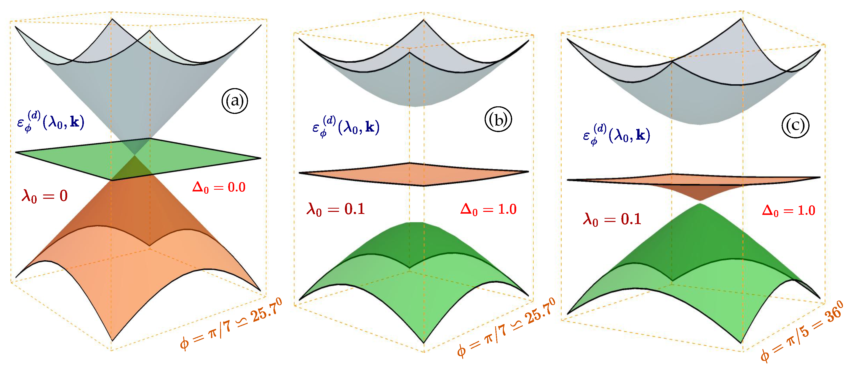
Figure 2.
(Color online) Energy dispersions for the model, a gapped diced lattice, and a Lieb lattice. All three materials exhibit a flat band, however, the location of this flat band is substantially different for each lattice.
Figure 2.
(Color online) Energy dispersions for the model, a gapped diced lattice, and a Lieb lattice. All three materials exhibit a flat band, however, the location of this flat band is substantially different for each lattice.
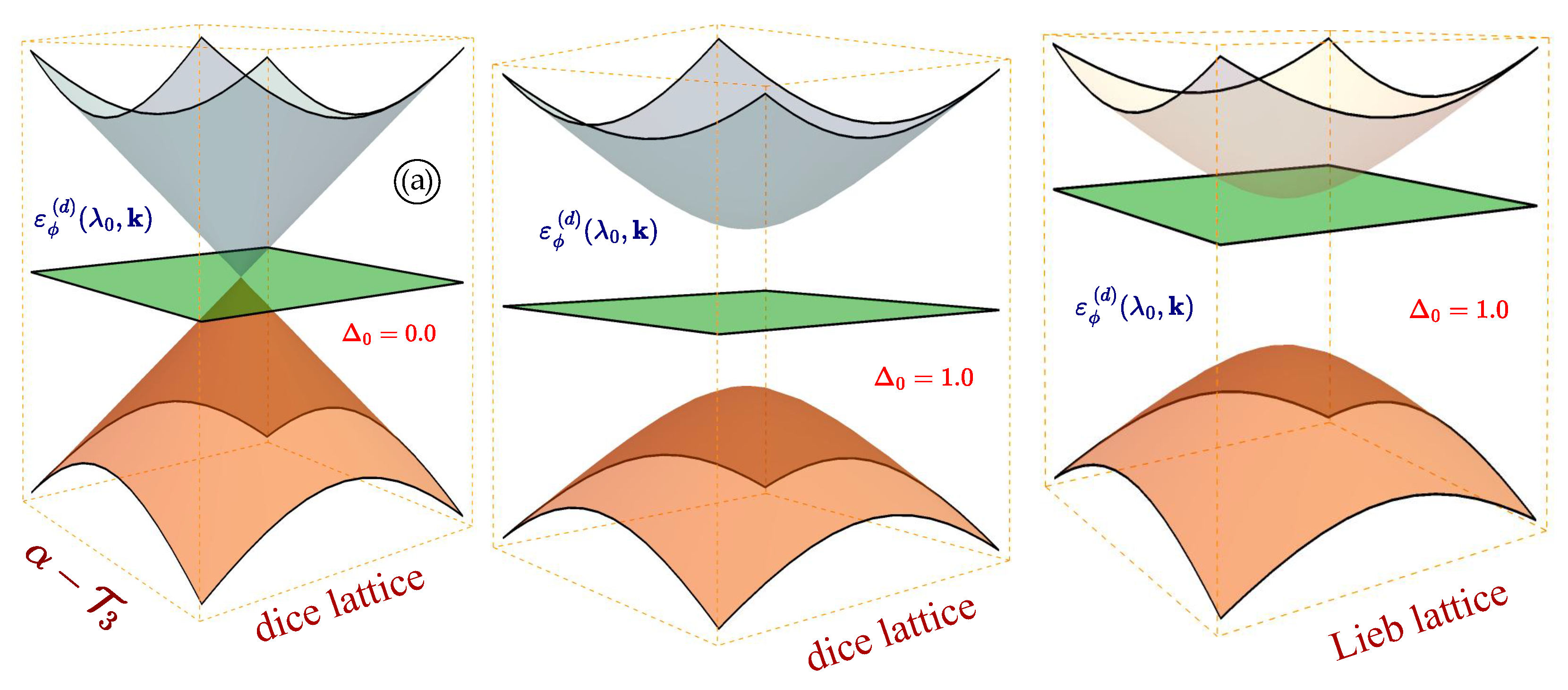
Figure 3.
(Color online) The -dependence of the energy dispersions for materials. Each panel corresponds to a zero bandgap and a fixed phase and different value of the coupling constant , as labeled. All the upper plots , and are related to the K valley with , the lower ones - to the valley with .
Figure 3.
(Color online) The -dependence of the energy dispersions for materials. Each panel corresponds to a zero bandgap and a fixed phase and different value of the coupling constant , as labeled. All the upper plots , and are related to the K valley with , the lower ones - to the valley with .
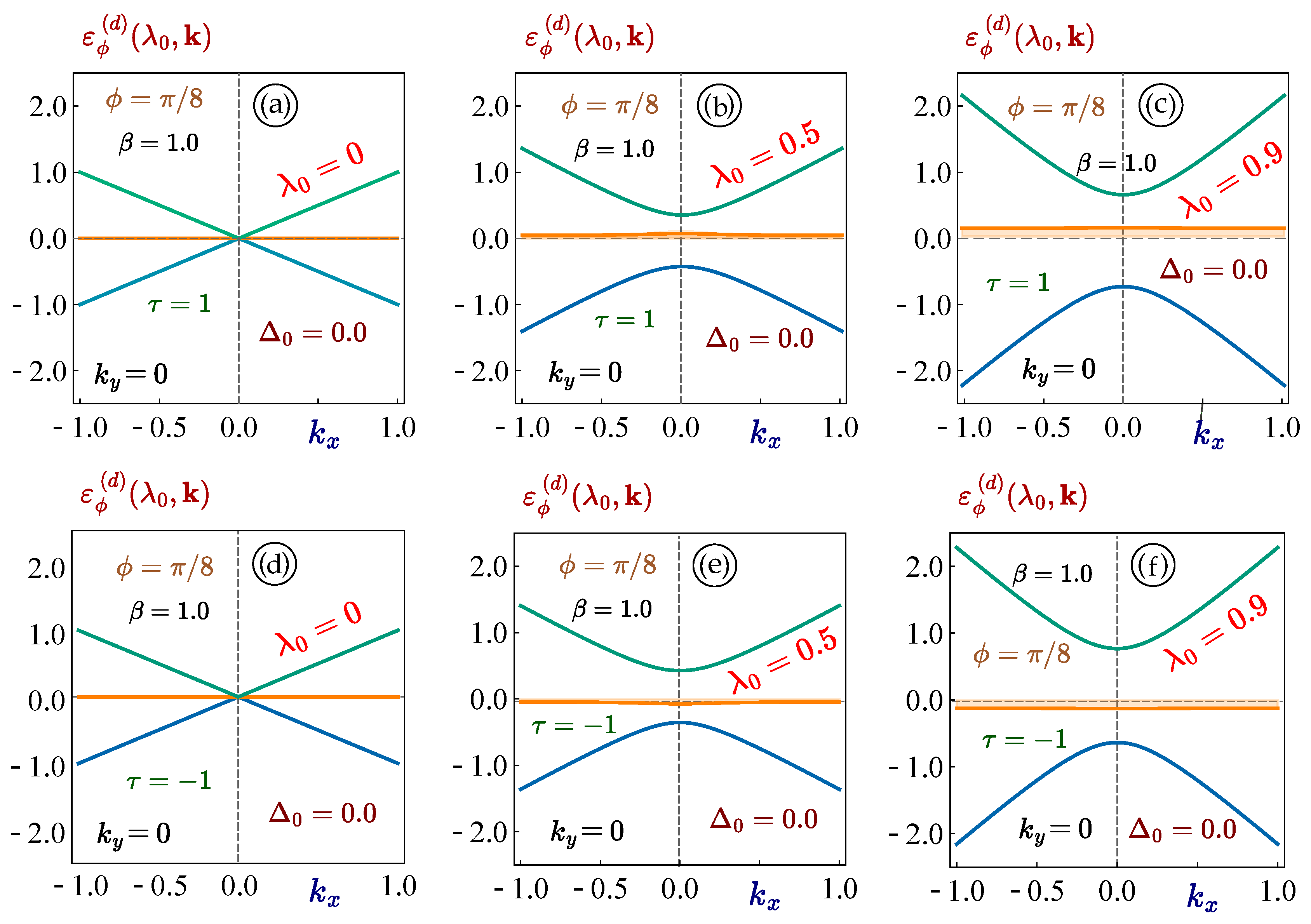
Figure 4.
(Color online) The -dependence of the energy dispersions for materials. Each panel corresponds to a finite bandgap and a fixed phase and different value of the coupling constant , as labeled. All the upper plots , and are related to the K valley with , the lower ones - to the valley with .
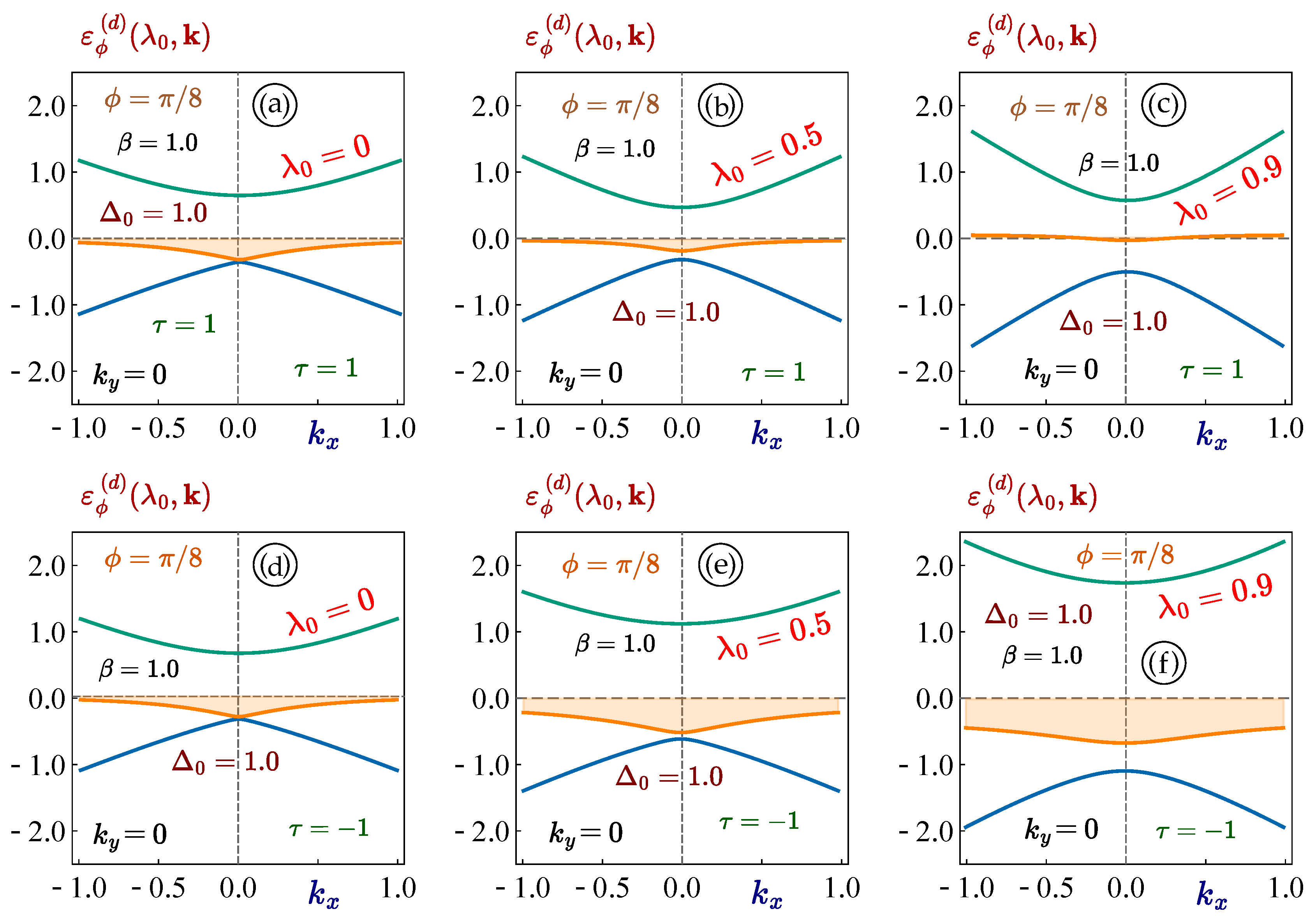
Figure 5.
(Color online) The -dependence of the energy dispersions for materials. Each panel describes a material with bandgap and electron-light coupling parameter and a specific phase according to our labeling.
Figure 5.
(Color online) The -dependence of the energy dispersions for materials. Each panel describes a material with bandgap and electron-light coupling parameter and a specific phase according to our labeling.
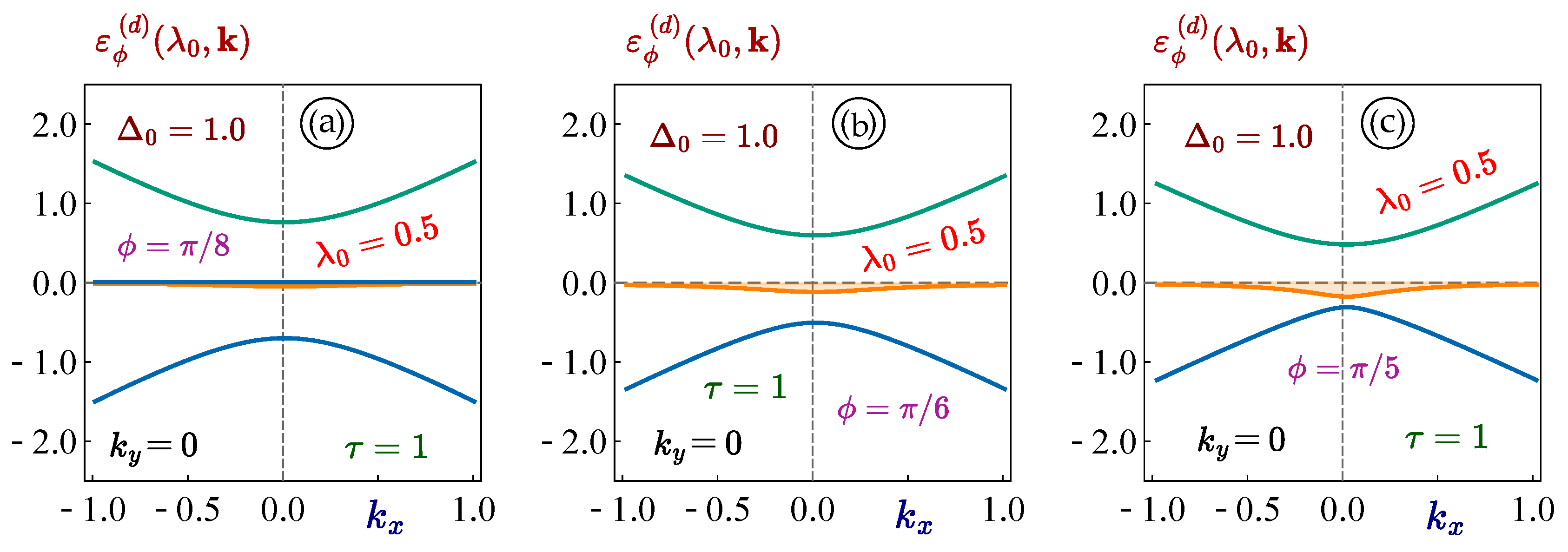
Figure 6.
(Color online) Angular dependence of the constant energy cut of the dispersions of materials in the presence of an elliptically polarized dressing field. The two curves in each panel corresponds to - an isotropic circularly polarized light (red curve), and strongly anisotropic elliptically polarized irradiation with (green curve). Panel is related to a phase , while plot - to a dice lattice with . We have considered a finite bandgap and coupling parameter for both panels.
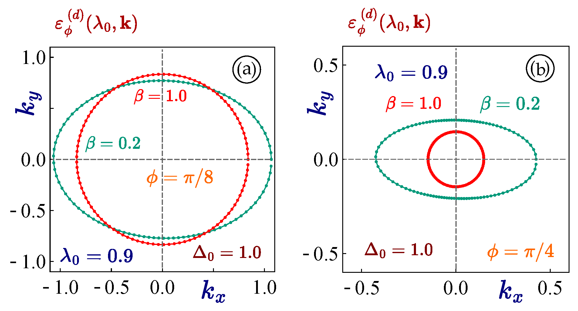
Figure 7.
(Color online) The -dependence of the energy dispersions for a Lieb lattice. Each panel describes a material with bandgap and a selected value of the coupling parameter , as labeled. Specifically, we demonstrate the modification and the finite dispersions the flat band due to the irradiation. Circularly polarzied dressing field with was selected for all panels.
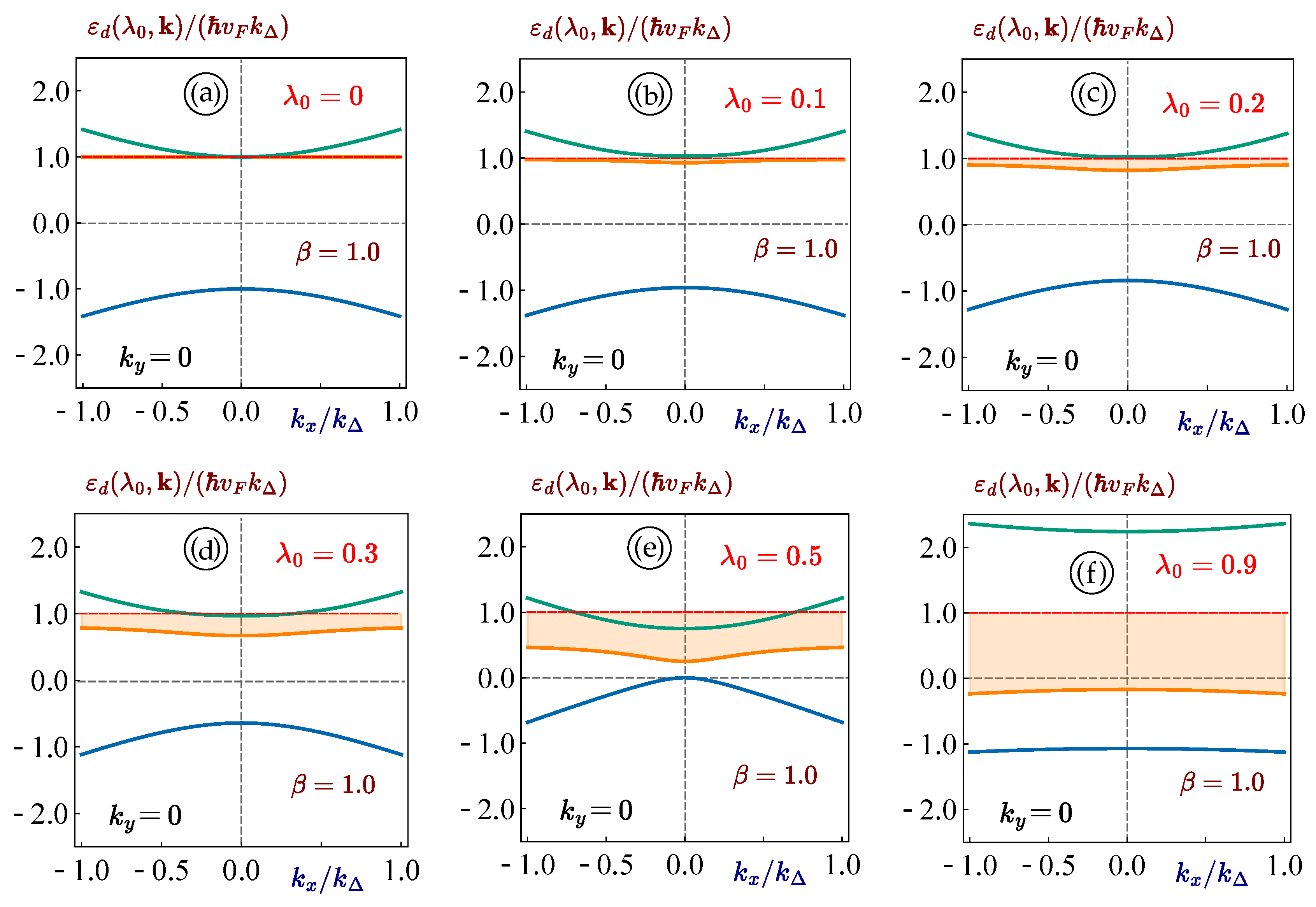
Figure 8.
(Color online) Three dimensional plots for the energy bandstructure for a Lieb lattice. Each panel describes a material with bandgap and a specific value of the coupling parameter , as labeled.
Figure 8.
(Color online) Three dimensional plots for the energy bandstructure for a Lieb lattice. Each panel describes a material with bandgap and a specific value of the coupling parameter , as labeled.
Disclaimer/Publisher’s Note: The statements, opinions and data contained in all publications are solely those of the individual author(s) and contributor(s) and not of MDPI and/or the editor(s). MDPI and/or the editor(s) disclaim responsibility for any injury to people or property resulting from any ideas, methods, instructions or products referred to in the content. |
© 2024 by the authors. Licensee MDPI, Basel, Switzerland. This article is an open access article distributed under the terms and conditions of the Creative Commons Attribution (CC BY) license (http://creativecommons.org/licenses/by/4.0/).
Copyright: This open access article is published under a Creative Commons CC BY 4.0 license, which permit the free download, distribution, and reuse, provided that the author and preprint are cited in any reuse.


