
Submitted:
10 June 2024
Posted:
11 June 2024
You are already at the latest version
Abstract
The inverse system identification toolbox named INVSID 1.0 for MATLAB, which is used to identify the inversion of single-input single-output systems, is developed. The complete process of developing the toolbox is demonstrated. Afterwards, a numerical example is illustrated to describe how the toolbox can be used to solve inverse identification problems. Simulation results demonstrate the effectiveness of the toolbox.
Keywords:
System inversion
; Inverse system identification
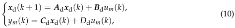
; MATLAB toolbox
1. Introduction
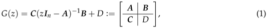
Nowadays, in many motion control systems, the requirements of high performance such as short motion times and small settling times. To fulfill these demands, combing feedback with feedforward control is normally implemented [1]. Figure 1 displays how a feedforward controller can be involved in feedback control systems, totally there are two kinds of modes. The feedback controller guarantees stability and improves disturbance rejection, while the feedforward controller enhances tracking performance such that the feedforward controller should be designed as (in the first mode) and (in the second mode), where the symbol “” denotes the Moore-Penrose pseudo inverse [2]. So system inversion is the key to the problem of feedforward control. Actually, in addition to applications in control systems, system inversion is frequently used in the areas of sensor calibration, loudspeaker linearization, digital predistortion for radio frequency communications, and so on [3]. So system inversion plays an important role in various research areas.
System inversion can be conducted by direct inversion and indirect inversion [4]. There exists several kinds of intrinsic limitations of direct inversion approaches, here an example is used to illustrate this, denote the transfer function of a finite-dimensional, discrete-time, single-input single-output, linear, constant dynamical system as
 where , , , , denotes an n-dimensional identity matrix, and is a state-space realization of . Based on (1), the inversion of can be represented as [5]
where , , , , denotes an n-dimensional identity matrix, and is a state-space realization of . Based on (1), the inversion of can be represented as [5]
There are at least two challenges in the direct inversion (2): (i) when does not exist, the direct inversion cannot be conducted; (ii) when there exist nonminimum-phase zeros1 in , the inversion will be unstable.
Due to the limitations of direct inversion approaches, various indirect inversion approaches have thus been proposed. A possible classification of existing indirect system inversion approaches consists in distinguishing between preview-based and non-preview-based approaches [4,6]:
- (a)
- Preview-based inversion approaches can be further categorized into infinite preview-based approaches and finite preview-based approaches. Infinite preview-based approaches admit an exact stable inversion solution, however, such a solution may require an infinite pre-actuation [7,8,9,10]. Because the length of the pre-actuation is proportional to the length of the desired output preview, infinite preview-based approaches is not applicable from a practical point of view. To handel the problem of applicability, finite preview-based approaches have been proposed [11,12,13,14,15,16,17,18].
- (b)
- Non-preview-based inversion approaches are preferred in practice. A family of approaches called pseudo-inversion, which can be conducted without preview, has been proposed [19,20]. However, such approaches will encounter other problems such as the difficulty of choosing a suitable basis function; Direct system identification-based inversion approaches the input-output data from the system to be inverted to identify the inverse system directly, however, the system identification cannot be conducted when the system to be inverted not stable [3]; For signal modeling-based inversion approaches, the input signal, which is to be reconstructed, must be a periodic signal under stationary operating conditions [21,22].
It should be noted that guaranteeing the stability of obtained solutions is a priority of both direct and indirect inversion approaches. So for some indirect inversion approaches, stability is ensured, but infinite or finite pre-actuation is needed.
In this paper, an entirely different system inversion approach by combing time-domain observer design and frequency-domain subspace identification is proposed. The presented approach can guarantee the stability of obtained system inversion, and simultaneously the proposed approach does not need any pre-actuation; Furthermore, the approach can be applied to stable or unstable, proper or improper systems2 to be inverted, and there is also no requirement for the type of input and output signals. Furthermore, it does not suffer non-convex or input noise problems.
To facilitate the use of the proposed system inversion approach by third parties, a MATLAB toolbox implementing the approach is created in this paper after theoretical derivation of the approach. The full name of the MATLAB toolbox is INVerse System IDentification with the first version which is abbreviated as INVSID 1.0.
The remainder of the paper is organized as follows. In Section 2, the inversion approach is proposed, and corresponding MATLAB codes are generated, based on which the toolbox NIVSID 1.0 is created, followed by Section 3, in which the usage of the toolbox NIVSID 1.0 is validated by a numerical example. Finally conclusions and future perspectives are given in Section 4.
2. Creation of INVSID 1.0
This section is illustrated by using three subsections with a progressive relationship: the proposed inverse identification approach is first presented, on the basis of which the corresponding MATLAB codes and the toolbox INVSID 1.0 are finally created. It should be noted that the toolbox INVSID 1.0 is only used for the inverse identification of single-input single-out systems.
2.1. Inverse Identification Approach
Given a finite-dimensional, discrete-time, single-input single-output, linear, constant dynamical system which is minimal-realized3 and proper, the given system can be either stable or unstable, and the sampling period of system is in seconds.
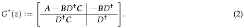
Figure 2 is used to demonstrate the basic idea behind the proposed inverse system identification approach, based on which the inverse model of the nominal model can be derived. As can be seen in Figure 2, the proposed approach mainly consists of five steps:
- (a)
- Obtain a state-space representation of the nominal system .
- (b)
- Given a number of sine signals , , corresponding to a number of N specified frequencies, and model them in state-space representation such that N signal models , , can be obtained.
- (c)
- By combing the signal models for with the model , respectively, the augmented models , , can be obtained. Then based on using the observers for the augmented models , , inverse models with , which can be used for reconstructing the input signals , , can be obtained.
- (d)
- Use frequency-domain system identification approaches to identify the inverse model of based on the frequency response function values of the models with at specified frequencies.
- (e)
- Choose the best inverse model by validating the identified inverse models.
The above steps are discussed in detail as follows:
- Step 1
- If the transfer function of the system is denoted as , and represents a minimal realization of , the corresponding state-space model of the system can be represented as
 where is the state vector of the model (3), and are the input and output of the system , respectively.
Remark 1.Actually, the proposed inverse identification approach is not limited to proper systems, the approach can also be used for identifying inversion of improper systems by replacing the present input by future input in (3).
where is the state vector of the model (3), and are the input and output of the system , respectively.
Remark 1.Actually, the proposed inverse identification approach is not limited to proper systems, the approach can also be used for identifying inversion of improper systems by replacing the present input by future input in (3). - Step 2
- Given a set S containing N discrete-time sine signals:wherewhere denotes the ordinary frequency in Hz, and the sequence is an arithmetic sequence, each sine wave in the set S can be represented as the output of a state-space model , i.e.,
 where denotes the state vector of the model (6), the matrices and can be denoted as
andrespectively.Remark 2.The frequencies of the signal , , in the set S can be specified by the following rule:where is a non-negative value, and d is a positive value.The rule in Equation (9) is not the only way to specify the frequencies.The values of for belong to the range with .
where denotes the state vector of the model (6), the matrices and can be denoted as
andrespectively.Remark 2.The frequencies of the signal , , in the set S can be specified by the following rule:where is a non-negative value, and d is a positive value.The rule in Equation (9) is not the only way to specify the frequencies.The values of for belong to the range with . - Step 3
-
If the signal is used as the input signal of the model (3), we can obtain
 where denotes the output of the model (3) when the input signal is .By augmenting the model (10) with the state vector of the model (6), an augmented model can be obtained, and it can be represented as
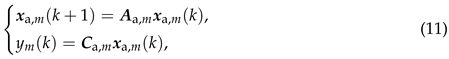 where the state vector can be denoted as
and the matrices and can be denoted asandrespectively.Based on the state-space model representation (11) for the augmented models , , we can totally build N full-order observers corresponding to the augmented models , , and we denote the m-th observer for the m-th augmented model as which can be described bywhere denotes the observer gain, and denotes the reconstructed value of using the observer.With the reconstructed value , we can obtain the reconstructed value of which can be calculated by the following equation:whereBy combing (15) with (16), we can get a state-space model
where the state vector can be denoted as
and the matrices and can be denoted asandrespectively.Based on the state-space model representation (11) for the augmented models , , we can totally build N full-order observers corresponding to the augmented models , , and we denote the m-th observer for the m-th augmented model as which can be described bywhere denotes the observer gain, and denotes the reconstructed value of using the observer.With the reconstructed value , we can obtain the reconstructed value of which can be calculated by the following equation:whereBy combing (15) with (16), we can get a state-space model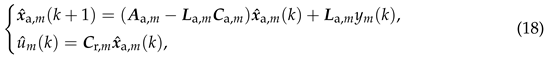 which can be regarded as a reconstructor of the input of the model (10).Let the model (18) be denoted as , and the value of the frequency response function of the model at the frequency can then be represented as where .
 - Step 4
- Let the inverse model of the model be denoted as , and with the frequency response function values , , the inverse model in state-space representation can be identified by using the subspace-based system identification method in frequency domain [23]. After system identification, the identified inverse model is denoted as .Remark 3.The effective frequency range of the inverse model can be specified by selecting the range of the frequencies of the signals , , in the set S.
- Step 5
-
Connect the models and in series, and the resulted model can be represented asof which the frequency response function is written aswhere with f the ordinary frequency in Hz, so if the identified inverse model is perfect, the frequency response of the model should satisfy:
- (a)
- .
- (b)
- .
By observing whether the frequency response function of the model within the frequency range specified by inverse system identification satisfies the above conditions (a) and (b) and to what extent it satisfies, the goodness of the identified inverse model can be validated.
2.2. MATLAB Codes
The corresponding MATLAB (R2020b) commands to realize the above inverse identification approach are illustrated step by step:
- Step 1
-
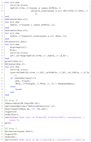
Given the transfer function of a nominal model , make a state-space realization of the transfer function:>> systf=tf(numerator,denominator,Ts);>> sysss=ss(systf);>> Figure (1);>> opts=bodeoptions;>> opts.FreqUnits=’Hz’;>> bode(sysss,opts);>> set(title(’Bode plot of ’),’interpreter’,’latex’);>> grid;
- Step 2
-
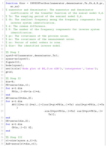
According to the bandwidth of the nominal model , specify the frequencies , , using the rule stated in Remark 2 and Remark 3, and stack all the frequencies into the vector , i.e.,Based on Equation (7) and Equation (8), create the matrices and for in the models of the N discrete-time sine signals in the set S, and stack them into the matrices and , respectively, i.e.,andso we can get the following MATLAB codes correspondingly:>> dim=N;>> FN=zeros(dim,1);>> for m=1:dimFN(m,:)=fb+(m-1)*d;end>> AN=zeros(2*dim,2);>> for m=1:dimAN(((2*m-1):2*m),:)=[cos(2*pi*FN(m,:)*Ts) sin(2*pi*FN(m,:)*Ts)AN(((2*m-1):2*m),:)=[-sin(2*pi*FN(m,:)*Ts) cos(2*pi*FN(m,:)*Ts)];end>> CN=zeros(dim,2);>> for m=1:dimCN(m,:)=[1 0];end
- Step 3
-
With the created matrices and for , create the matrices , , and for by using Equation (13), Equation (14), and Equation (17), respectively. Then stack the matrices and , , into the matrices , , and , respectively, i.e.,andBased on the expression of the model (18), calculate the transfer function of the reconstructors by usingwhere the observer gain can be chosen in a linear least-squares sense for stochastic systems, i.e., the observer gain can be obtained as the gain of the steady-state Kalman filter for the model (11) with process noise and measurement noise or can be obtained in a minimum mean-integral squared error sense [24], denote the process noise and measurement noise as with and , respectively, and assume that both and are white Gaussian sequences, with Q > 0, with , and assume that the distribution of is Gaussian, and assume that and are uncorrelated with and with each other. Then derive the gain of the steady-state Kalman filter for the model (11) by using the following equation [25]where the value of can be derived as the unique solution of the following algebraic Riccati equationunder the following conditions:
- (a)
- is detectable4.
- (b)
- is controllable.
Then stack all the calculated observer gains for into the matrix , i.e.,After calculating the reconstructor transfer functions for based on (27), stack all the obtained transfer functions into the vector function which can be denoted asObtain the frequency response function values for by replacing z in Equation (27) with for , then stack all the frequency response function values into the vector , i.e.,The above process can be realized by the following MATLAB codes:>> r1=size(sysss.a,1)+2;>> AaN=zeros(r1*dim,r1);>> for m=1:dimr2=1+(m-1)*r1;AaN(r2:r1*m,:)=[sysss.a sysss.b*CN(m,:)AaN(r2:r1*m,:)=[zeros(2,size(sysss.a,1)) AN(((2*m-1):2*m),:)];end>> CaN=zeros(dim,r1);>> for m=1:dimCaN(m,:)=[sysss.c sysss.d*CN(m,:)];end>> CrN=zeros(dim,r1);>> for m=1:dimCrN(m,:)=[zeros(1,size(sysss.a,1)) CN(m,:)];end>> LN=zeros(r1,dim);>> for m=1:dimQ=qc*eye(r1);R=mc;sysa=ss(AaN(r2:r1*m,:),zeros(r1,r1),CaN(m,:),zeros(1,r1),Ts);[∼,LN(:,m),∼]=kalman(sysa,Q,R);end>> g=cell(dim,1);>> GN=zeros(dim,1);>> for m=1:dimr2=1+(m-1)*r1;sysr=ss(AaN(r2:r1*m,:)-LN(:,m)*CaN(m,:),LN(:,m),CrN(m,:),0,Ts);if isstable(sysr)==1g{m,:}=sysr;GN(m,:)=frd(g{m,:},FN(m,:),’Hz’).ResponseData;elsebreakendRemark 4.The values of Q and R can be tuned by changing the values of pc and mc. - Step 4
-
With the calculated frequency response function values , , the inverse model in state-space representation can be identified by using the MATLAB function n4sid:>> fdata=idfrd(GN,2*pi*FN,Ts);>> opt=n4sidOptions("EnforceStability",1);>> Ginv=n4sid(fdata,nx,’Ts’,Ts,opt);>> figure;>> opts=bodeoptions;>> opts.FreqUnits=’Hz’;>> bode(Ginv,opts);>> set(title(’Bode plot of ’),’interpreter’,’latex’);>> grid;Remark 5.The values of nx denotes the inverse model order which can be specified.
- Step 5
-
The following MATLAB command can be used for the series connection of the models and .>> Gs=series(sysss,Ginv);Then the Bode plot of the combined model can be displayed using:>> figure;>> opts=bodeoptions;>> opts.FreqUnits=’Hz’;>> bode(Gs,opts);>> set(title(’Bode plot of ’),’interpreter’,’latex’);>> grid;
2.3. Inverse System Identification Toolbox Creation
Building the inverse system identification toolbox consists of two parts:
- Part 1
-
Based on the MATLAB codes of inverse identification obtained in Section 2.2, a MATLAB function file, which is an m-file, can be created. The specific content of the m-file is given as follows.

- Part 2
- With the MATLAB m-file created in the first part, the inverse system identification toolbox INVSID 1.0 can be installed, the complete installation procedure contains five steps from the first step about the selection of the item Package Toolbox from the Add-Ons menu to the end step about saving the created toolbox5.
3. Numerical Studies
In this section, two numerical examples are used for validate the effectiveness of the toolbox INSID 1.0, i.e., check the effectiveness of the proposed inverse system identification approach.
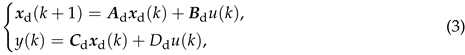
Firstly, given a discrete-time, single-input single-output, linear, constant dynamical system of which the transfer function is described by
with the sampling period seconds, and the Bode plot of the system is displayed in Figure 3.
According to the transfer function (34), the following observations can be made:
- (a)
- is stable.
- (b)
- is proper.
- (c)
- is minimal-realized.
- (d)
- has a nonminimum-phase zero.
According to the above observations, it can be known that the direct inversion of the system G is a challenging problem. So now turn to using the proposed toolbox INVSID 1.0 to identify the inverse model of the system G. The proposed inverse identification approach can specify the frequency range of interest, i.e., by selecting the values of , m, and d in Equation (20), the frequency range to be identified can be determined. The parameters showed in Table 1 are used as the inputs of the inverse identification toolbox.
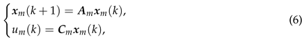
With the above inputs, the final output of the inverse identification toolbox is the identified inverse model which is the best model corresponding to the recommended singular value. The model order of the identified inverse model is recommended to be 4. The frequency response properties of the model with fourth order is demonstrated in Figure 4.
In addition, the inversion is identified using the MATLAB function n4sid with stability enforcement, so the identified model is stable and causal.
By connecting the model and the model in series using Equation (19), the model can be obtained. The obtained model can then be used for validating the goodness of the identified inverse model in the frequency range of interest. The frequency response of the obtained model is shown in Figure 5, in the specified frequency range from 10 Hz to 500 Hz, the magnitude is nearly a constant near to 0 dB, and the phase is nearly a constant around 0 degrees. The values of magnitude and phase can indicate the effectiveness of the proposed inverse identification toolbox for stable systems to be inverted.
In practice, unstable systems are also frequently encountered. So the second numerical example is about using the toolbox INVSID 1.0 to solve system inversion problem of an unstable system.
Given a discrete-time, single-input single-output, linear, constant dynamical system of which the transfer function is described by
with the sampling period seconds, and the Bode plot of the system is displayed in Figure 6.
According to the transfer function (34), the following observations can be made:
- (a)
- is unstable.
- (b)
- is proper.
- (c)
- is minimal-realized.
- (d)
- has a nonminimum-phase zero.
The parameters showed in Table 2 are used as the inputs of the inverse identification toolbox.
With the above inputs, the final output of the inverse identification toolbox is the identified inverse model which is the best model corresponding to the recommended singular value. The model order of the identified inverse model is recommended to be 4. The frequency response properties of the model with fourth order is demonstrated in Figure 7.
In addition, the inversion is identified using the MATLAB function n4sid with stability enforcement, so the identified model is stable and causal.
By connecting the model and the model in series using Equation (19), the model can be obtained. The frequency response of the obtained model is shown in Figure 8, in the specified frequency range from 10 Hz to 500 Hz, the magnitude is nearly a constant near to 0 dB, and the phase is nearly a constant around 0 degrees. The values of magnitude and phase can indicate the effectiveness of the proposed inverse identification toolbox for unstable systems to be inverted.
4. Conclusion and Outlook
In this paper, an alternative system inversion approach is proposed, and based on which the toolbox named INVSID 1.0 is developed. The advantages of the toolbox INVSID 1.0 can be concluded as follows:
- (a)
- The proposed inverse identification toolbox can be used for stable or unstable systems.
- (b)
- Preview is not needed.
- (c)
- The frequency range of interest can be specified.
- (d)
- Stability of the identified inverse model can be guaranteed.
- (e)
- Subspace identification is used such that there is no non-convex problem.
Furthermore, according to the theoretical derivation of the proposed system inversion approach, it can be indicated that the proposed approach can be used for systems with noise, because an observer is involved in the approach.
Currently, the inverse identification toolbox INVSID 1.0 is used for single-input single-output systems, while in the future the proposed inverse system identification approach will be extended to identify the inverse models of general multiple-input multiple-output systems such that more advanced versions of the INVSID toolbox can be created.
Author Contributions
Conceptualization, R.H.; methodology, R.H.; software, R.H.; validation, R.H.; formal analysis, R.H.; investigation, R.H.; resources, R.H.; data curation, R.H.; writing—original draft preparation, R.H.; writing—review and editing, R.H., C.B. and G.B.; visualization, R.H.; supervision, R.H.; project administration, R.H.; funding acquisition, R.H. All authors have read and agreed to the published version of the manuscript.
Funding
This research was funded by the Natural Science Foundation of Zhejiang pvovince, P.R. China (Grant No. LQ23F030005) and the University Research Development Foundation in Zhejiang A&F University, P.R. China (Grant No. 203402000601).
Funding
This research was funded by the Natural Science Foundation of Zhejiang pvovince, P.R. China (Grant No. LQ23F030005) and the University Research Development Foundation in Zhejiang A&F University, P.R. China (Grant No. 203402000601).
References
- Goodwin, G.C.; Graebe, S.F.; Salgado, M.E. Control System Design; Upper Saddle River, NJ: Prentice Hall, 2001. [Google Scholar]
- Golub, G.H.; Van Loan, C.F. Matrix Computations; John Hopkins University Press, MD: Baltimore, 2012. [Google Scholar]
- Jung, Y. Inverse System Identification with Applications in Predistortion; Linköping University, Sweden: Linköping, 2018. [Google Scholar]
- van Zundert, J.; Oomen, T. On inversion-based approaches for feedforward and ILC. Mechatronics 2018, 50, 282–291. [Google Scholar] [CrossRef]
- Zhou, K.; Doyle, J.C.; Glover, K. Robust and Optimal Control; Prentice Hall, NJ: Englewood Cliffs, 1996. [Google Scholar]
- Rigney, L.Y.P.; Lawrence, D.A. Nonminimum phase dynamic inversion for settle time applications. IEEE Trans. Control Syst. Technol. 2009, 17, 989–1005. [Google Scholar] [CrossRef]
- Devasia, D.C.; Paden, B. Nonlinear inversion-based output tracking. IEEE Trans. Autom. Control 1996, 41, 930–942. [Google Scholar] [CrossRef]
- Hunt, L.; Meyer, G.; Su, R. Noncausal inverses for linear systems. IEEE Trans. Autom. Control 1996, 41, 608–611. [Google Scholar] [CrossRef]
- Widrow, B.; Walach, E. Adaptive Inverse Control: A Signal Processing Approach; John Wiley & Sons, NJ: Hoboken, 2008. [Google Scholar]
- Sogo, T. On the equivalence between stable inversion for nonminimum phase systems and reciprocal transfer functions defined by the two-sided Laplace transform. Automatica 2010, 46, 122–126. [Google Scholar] [CrossRef]
- Tomizuka, M. Zero phase error tracking algorithm for digital control. J. Dyn. Syst. Meas. Control 1987, 109, 65–68. [Google Scholar] [CrossRef]
- Gross, E.; Tomizuka, M.; Messner, W. Cancellation of discrete time unstable zeros by feedforward control. J. Dyn. Syst. Meas. Control 1994, 116, 33–38. [Google Scholar] [CrossRef]
- Roover, D.D.; Bosgra, O.H. Synthesis of robust multivariable iterative learning controllers with application to a wafer state motion system. Int. J. Control 2000, 73, 968–979. [Google Scholar] [CrossRef]
- Mirkin, L. On the H∞ fixed-lag smoothing: How to exploit the information preview. Automatica 2003, 39, 1495–1504. [Google Scholar] [CrossRef]
- Hazell, A.; Limebeer, D.J.N. An efficient algorithm for discrete-time H∞ preview control. Automatica 2008, 44, 2441–2448. [Google Scholar] [CrossRef]
- Zhang, Y.; Liu, S. Pre-actuation and optimal state to state transition based precise tracking for maximum phase system. Asian J. Control 2016, 18, 1–11. [Google Scholar] [CrossRef]
- Zhu, Q.; Zhang, Y.; Xiong, R. Stable inversion based precise tracking for periodic systems. Asian J. Control 2020, 22, 217–227. [Google Scholar] [CrossRef]
- Zou, Q. Optimal preview-based stable-inversion for output tracking of nonminimum-phase linear systems. Automatica 2020, 45, 230–237. [Google Scholar] [CrossRef]
- Jetto, L.; Orsini, V.; Romagnoli, R. Accurate output tracking for nonminimum phase nonhyperbolic and near nonhyperbolic systems. Eur. J. Control 2014, 20, 292–300. [Google Scholar] [CrossRef]
- Romagnoli, R.; Garone, E. A general framework for approximated model stable inversion. Automatica 2019, 101, 182–189. [Google Scholar] [CrossRef]
- Bohn, C.; Cortabarria, A.; Härtel, V.; Kowalczyk, K. Active control of engine-induced vibrations in automotive vehicles using disturbance observer gain scheduling. Control Eng. Pract. 2004, 12, 1029–1039. [Google Scholar] [CrossRef]
- Han, C.B.; Bauer, G. Comparison between calculated speed-based and sensor-fused speed-based engine in-cylinder pressure estimation method. IFAC-PapersOnLine 2022, 55, 223–228. [Google Scholar] [CrossRef]
- McKelvey, T.; Akçay, H.; Ljung, L. Subspace-based multivariable system identification from frequency response data. IEEE Trans. Autom. Control 1996, 41, 960–979. [Google Scholar] [CrossRef]
- O’Reilly, J. Observers for Linear Systems; Academic Press, UK: London, 1983. [Google Scholar]
- Lewis, F.L.; Xie, L.; Popa, D. Optimal and Robust Estimation: With an introduction to stochastic control theory; CRC Press, FL: Boca Raton, 2008. [Google Scholar]
| 1 | For discrete-time systems, nonminimum-phase zeros are zeros that lie outside the unit disk. |
| 2 | The system is proper when the degree of the numerator does not exceed the degree of the denominator of its transfer function, otherwise the system is improper. |
| 3 | The dynamical system is minimal-realized if and only if it is both controllable and observable. |
| 4 | A system is detectable if all the unobservable states are stable. |
| 5 | Installation procedure of MATLAB toolboxes can be referred to https://www.mathworks.com/help/matlab/matlabprog/create-and-share-custom-matlab-toolboxes.html. |
Figure 1.
Inverse model-based feedforward-feedback control (r: reference signal; F: feedforward controller; C: feedback controller; G: plant model; : closed-loop system model; e: error; f: feedforward controller output; y: control system output).
Figure 1.
Inverse model-based feedforward-feedback control (r: reference signal; F: feedforward controller; C: feedback controller; G: plant model; : closed-loop system model; e: error; f: feedforward controller output; y: control system output).
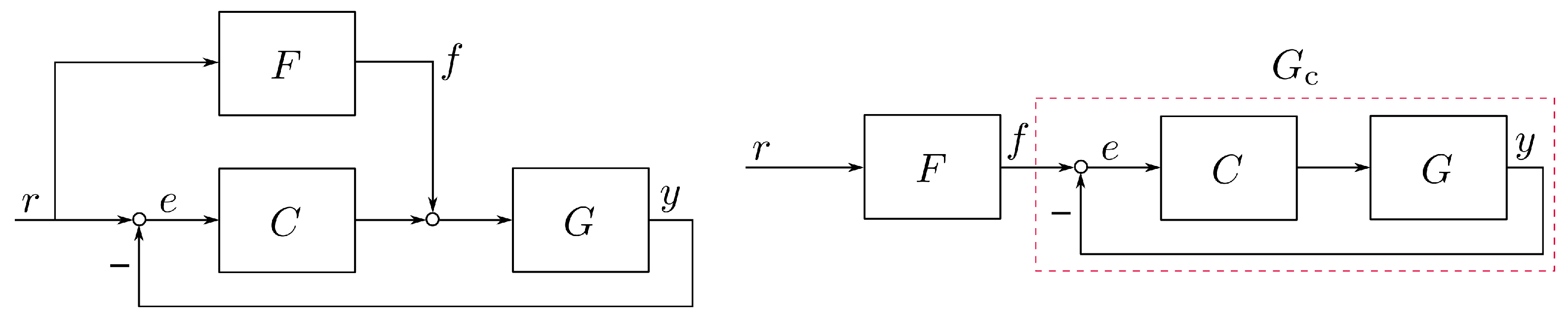
Figure 2.
Framework of proposed inverse system identification approach. (The symbol denotes reconstructed or estimated value.).
Figure 2.
Framework of proposed inverse system identification approach. (The symbol denotes reconstructed or estimated value.).

Figure 3.
Bode plot of .
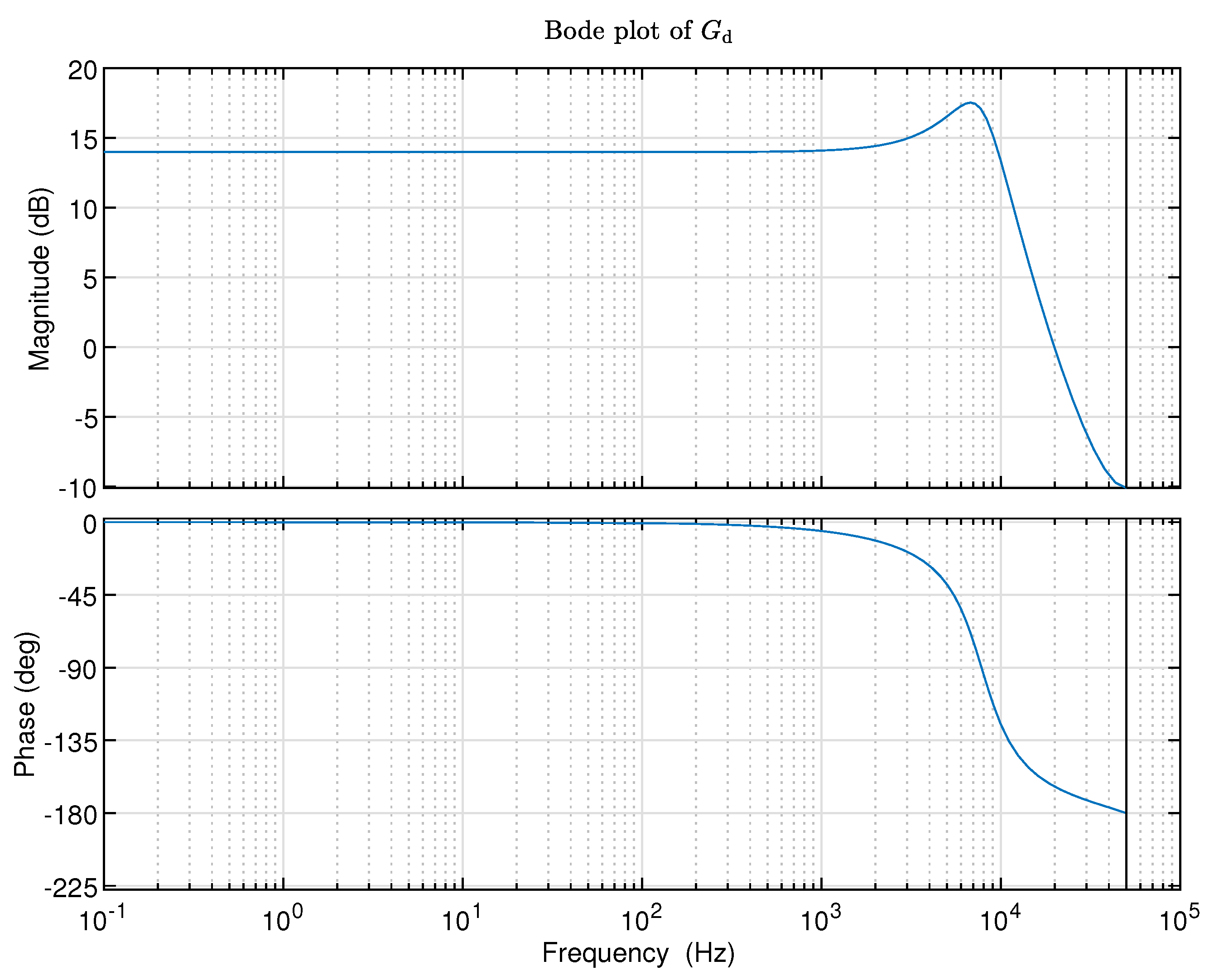
Figure 4.
Bode plot of .
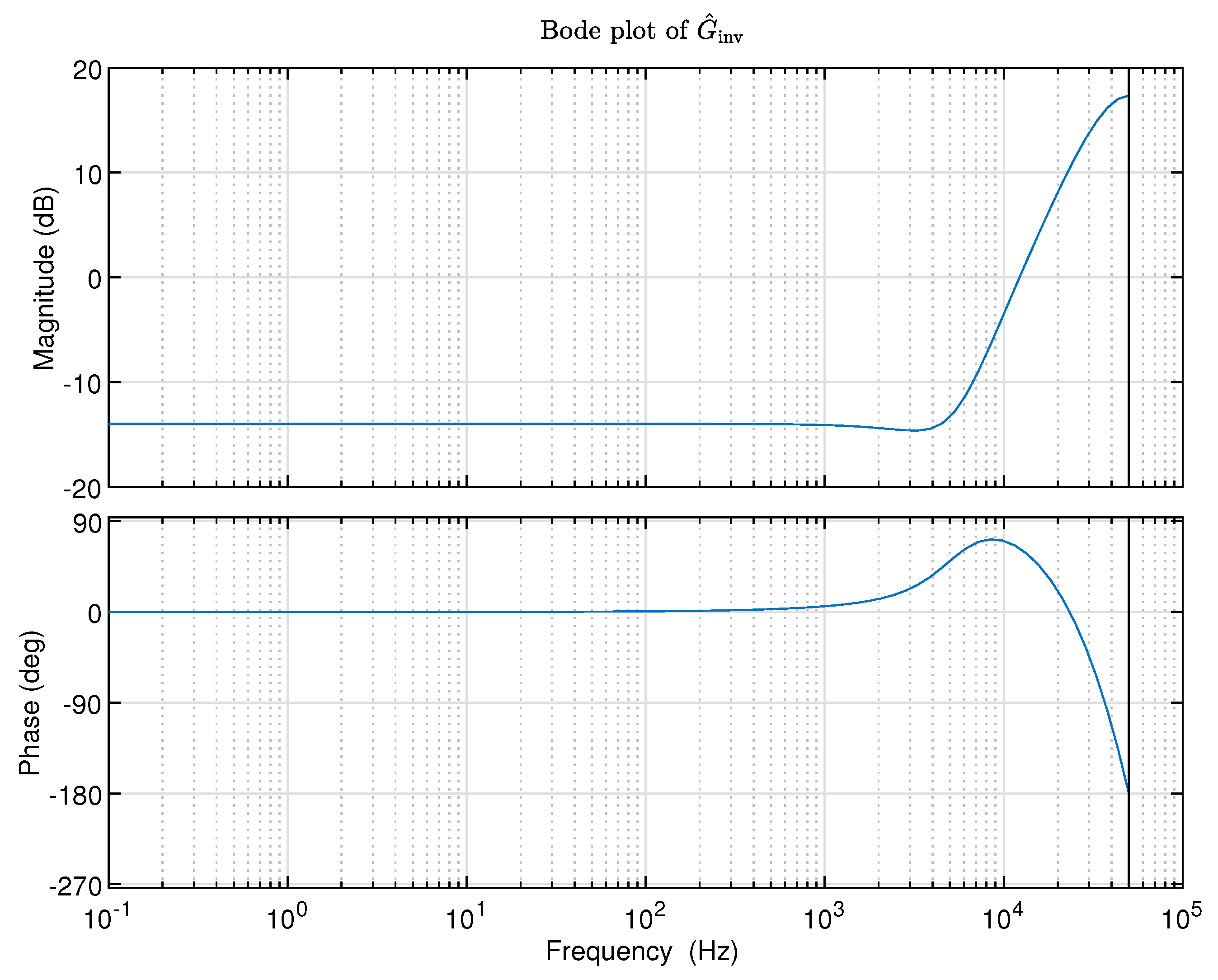
Figure 5.
Bode plot of .
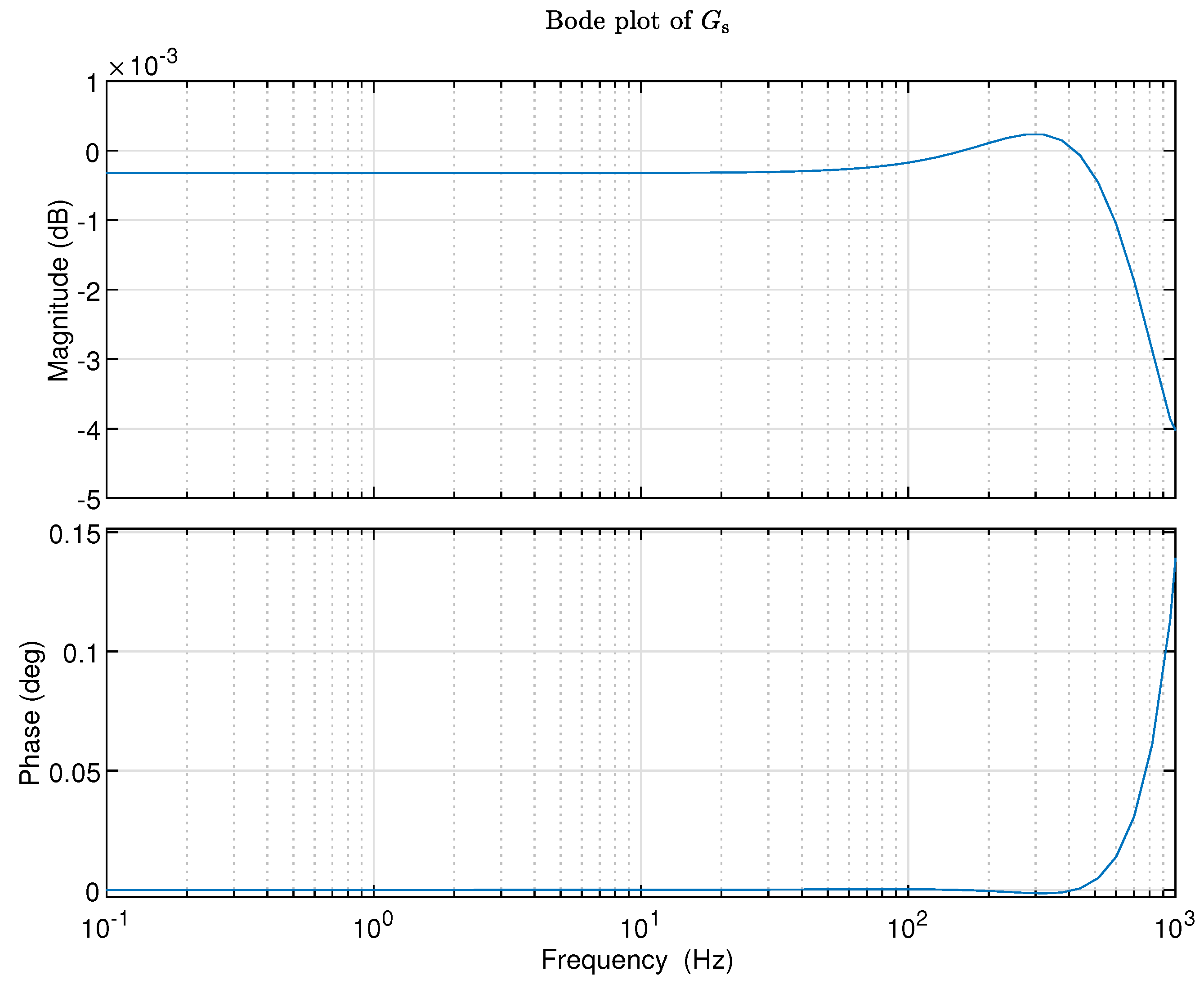
Figure 6.
Bode plot of .
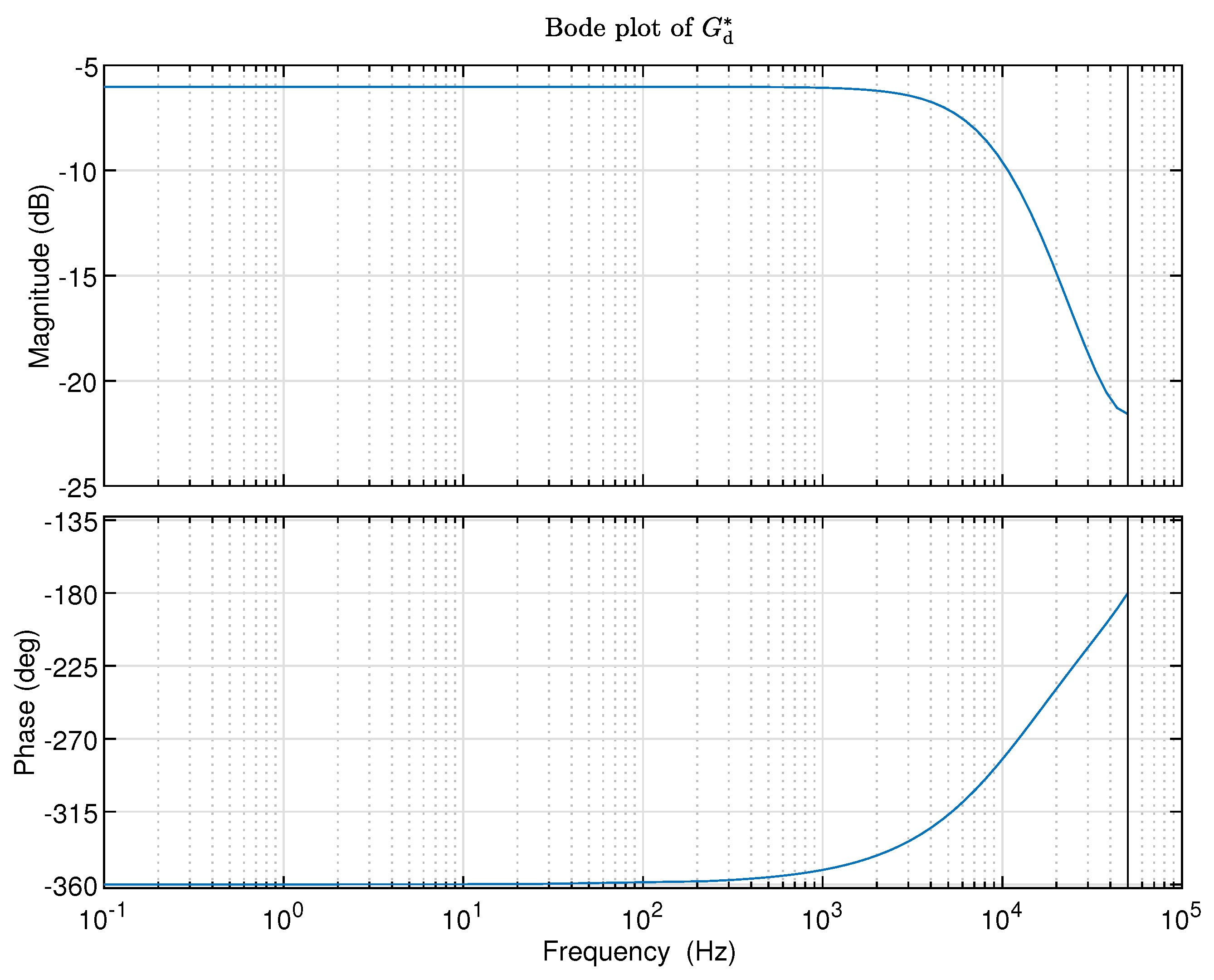
Figure 7.
Bode plot of .
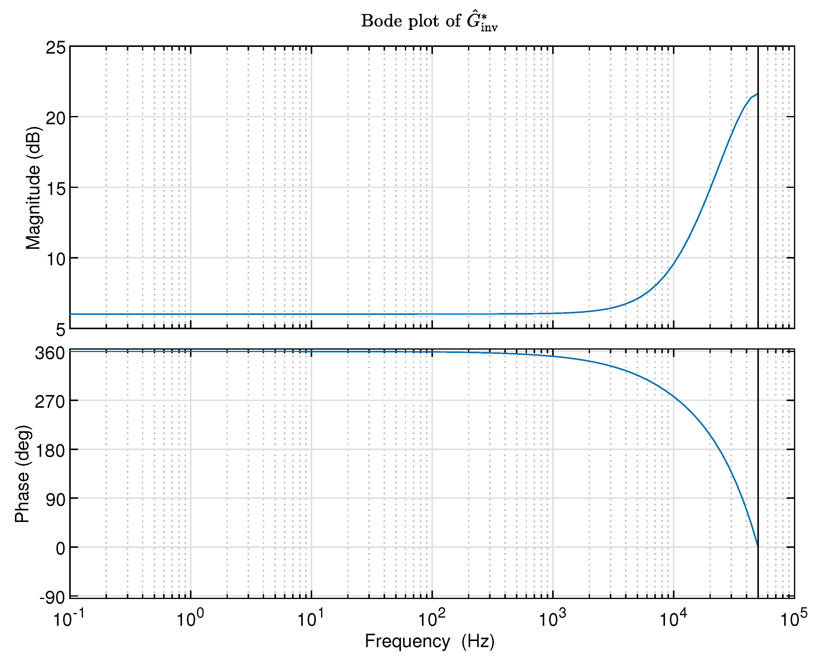
Figure 8.
Bode plot of .
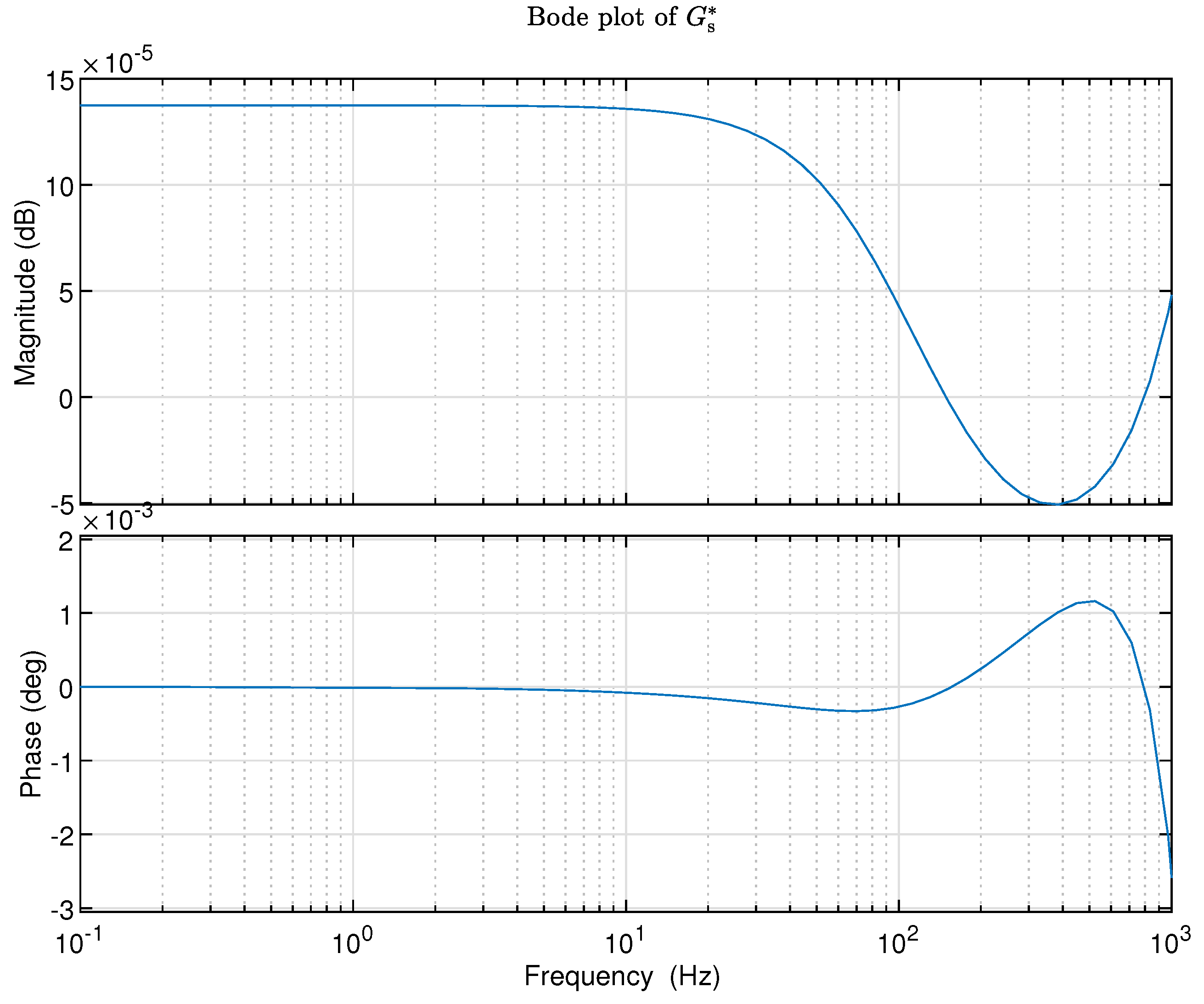

Table 1.
Parameters for inverse identification.
| Parameter | Value in MATLAB |
| numerator | [0,1,0] |
| denominator | [1,-1.5,0.7] |
| Ts | |
| fb | |
| d | |
| N | |
| pc | |
| mc | |
| nx |
Table 2.
Parameters for inverse identification.
| Parameter | Value in MATLAB |
| numerator | [0,1,0] |
| denominator | [1,-5,6] |
| Ts | |
| fb | |
| d | |
| N | |
| pc | |
| mc | |
| nx |
Disclaimer/Publisher’s Note: The statements, opinions and data contained in all publications are solely those of the individual author(s) and contributor(s) and not of MDPI and/or the editor(s). MDPI and/or the editor(s) disclaim responsibility for any injury to people or property resulting from any ideas, methods, instructions or products referred to in the content. |
© 2024 by the authors. Licensee MDPI, Basel, Switzerland. This article is an open access article distributed under the terms and conditions of the Creative Commons Attribution (CC BY) license (http://creativecommons.org/licenses/by/4.0/).
Copyright: This open access article is published under a Creative Commons CC BY 4.0 license, which permit the free download, distribution, and reuse, provided that the author and preprint are cited in any reuse.


