
Submitted:
31 May 2024
Posted:
04 June 2024
You are already at the latest version
Abstract
As the largest contributor of carbon emissions in China, the building sector currently relies mostly on enterprises’ own effort to report carbon emissions, which usually results in challenges related to information transparency and workload for regulatory bodies, who play an otherwise vital role in controlling the building sector’s carbon footprint. In this study, we established a novel regulatory model known as QCEPM (Quantitative Carbon Emission Prediction Model) by conducting multiple linear regression analysis using the quantities of concrete, rebar, and masonry structures as independent variables, and the embodied carbon emissions of a building as the dependent variable. We processed the data in the detailed quantity list of 20 multi-story frame-structure buildings and fed them to QCEPM for solution. Comparison of the QCEPM-calculated results against the time-consuming and error-prone manual calculation results suggested a mean absolute percentage error (MAPE) of 2.26%. Using this simplified model, regulatory bodies can efficiently supervise the embodied carbon emissions in multi-storey frame structures by setting up carbon quota for a project in its approval stage, allowing the construction enterprise to carry out dynamic control over the audited three most important building materials throughout a project’s planning and implementation phase.
Keywords:
Regulatory model
; Building LCA
; Embodied carbon emissions
; Low carbon construction technology
; Environmental impact assessment
1. Introduction
1.1. Global Warming: Consequences, Causes and Challenges
In 2022, the carbon dioxide emissions (in terms of carbon dioxide equivalent) generated from energy use, industrial processes, flaring, and methane emissions amounted to 39.3 Gt, representing a 0.8% increase from the previous year, reaching an all-time-high in history[1]. The warming caused by human greenhouse gas (GHG) emissions has resulted in anomalies in the climate system, including longer-lasting heatwave events globally [2], a continuous increase in the likelihood of droughts [3], significant increases in surface runoff and expansion of flood-affected areas [4,5], and a growing number of reports of extreme weather. This poses significant risks to ecosystems and human societies, such as altered water availability and threatened water security [6], causing irreversible harm to terrestrial, wetland, and marine ecosystems [7,8,9], challenging human societies with climate anxiety, and reducing the healthcare system’s ability to respond to climate-sensitive diseases [10]. Climate change has also severely impacted food/nutrition security and food production systems [11,12]. It is estimated that it is only possible to alter the global warming trend by containing the rise in the Earth’s median surface temperature within 1.5°C by the end of the 21st century, to achieve that, carbon neutrality has to be achieved by 2050 [13]. Over the past two decades, China's carbon emissions have seen rapid increase and currently accounts for 32.1% of global carbon emissions, with 50.9% of the Chinese total national carbon emissions consisting of carbon emissions from the construction industry[14]. However, there yet to be a reasonable and unified method for calculating carbon emissions in the Chinese construction industry, leading to difficulties in government regulation and undermotivated corporate participation, resulting in ineffective control over carbon emissions.
1.2. Common Practices for Analyzing Carbon Emissions
Through literature review, we identified 4 categories of methods for calculating carbon emissions in terms of emission composition analysis, deciding factors affecting carbon emissions, and prediction of carbon emissions.
1.2.1. Input-Output Analysis
Input-output analysis (IOA) is a method that utilizes mathematical approaches to investigate the quantitative relationships between inputs and outputs in a given system [15]. It has been employed to study and analyze the interdependencies between various sectors of the national economy in terms of the production and consumption of products. This method involves creating input-output models to trace the sources of carbon inputs and the destinations of carbon outputs across different sectors of the national economy, as well as the inter-sectoral connections related to carbon-providing or carbon-consuming products. IOA can be combined with various other methods and applied at different scales. For example, the mathematical structure of IOA is closely related to LCA [16,17,18] and is an important tool for research and application in the field of sustainability[19,20,21]. Since IOA requires the collection of extensive data from various industries, and data collection methods and timing vary significantly between different industries, this can lead to inaccurate assessments of carbon emissions [22]. Therefore, IOA is suitable for macro-level research spanning multiple regions, sectors, or countries.
1.2.2. Decomposition Analysis
Decomposition analysis is a method that decomposes comprehensive statistical metrics into several relatively independent and simpler portions to study the nature of changes. It has been used to investigate the driving factors of carbon emissions [23,24,25]. Commonly employed analysis models include Index Decomposition Analysis (IDA) [26] and Structural Decomposition Analysis (SDA) [27]. This method is a form of comparative static analysis, and is therefore less concerned with processes of change.
1.2.3. Econometrics
Econometrics is a method that uses mathematical and statistical approaches to determine specific quantitative relationships within economic contexts[28]. It has been applied to identify the impact factors of carbon emissions as well as each factor’s respective extent of impact [29]. The Stochastic Impacts by Regression on Population, Affluence, and Technology (STIRPAT) framework is widely used to examine the relationship between carbon emissions and impact factors [30] . It involves simulating different variables such as human behavior and economic activities to assess their impact on carbon emissions [31,32,33,34]. Econometrics is a complex computational process and may miss some key impact factors when identifying variables. Additionally, since the general form of econometrics is often a mathematical model with linear relationships between variables, issues like multicollinearity can arise, leading to significant errors in calculations [35].
1.2.4. Data Envelopment Analysis
Data envelopment analysis (DEA) is a quantitative analytical method that uses non-parametric programming to evaluate the relative efficiency of comparable units of the same type [36]. Common DEA models include CCR [37] and BCC [38]. This method is primarily used for assessing the efficiency of various decarbonization measures and providing optimization decisions or recommendations [39,40,41]. It is not used for carbon emissions calculations.
1.3. Problem Statement
The above methods all involve collecting adequate data and harnessing algorithmic approaches to tackle detailed and complex research inquiries, which would be impossible without having certain prerequisites in place. However, among China’s 143,446 construction enterprises in 2022, companies capable and willing to implement such prerequisites (usually fall under categories like state-owned enterprises, collective enterprises, and foreign-funded enterprises) account for only 4.66% and they are responsible for only 13.4% of the country's total construction area [42]. More projects are completed by small and medium-sized private enterprises with lower standardization and less capital investment. Therefore, the data collection and tracking mentioned in the above methods are not suitable for the current Chinese construction industry as the significant differences in the level of operation between each enterprise may result in considerable errors in the calculation results, making it difficult to formulate unified carbon emission management measures on the basis of these methods. The Chinese construction industry calls for a different carbon emissions measurement method, one that requires less additional investment and is relatively practical for all enterprises to implement.
From an auditing perspective, internationally recognized project-based carbon emissions accounting methods include real-time monitoring [43,44,45], mass balance [46,47], and emission factor [48,49] The principles, characteristics, and application scenarios of these three methods are outlined in Table 1.
For the regulatory bodies and the companies they regulate, real-time monitoring requires the deployment of monitoring equipment and dedicated personnel to track the carbon emissions throughout the construction process. The significant additional investment can lead to a lack of motivation for business participation, which is not conducive to regulation. The mass balance method focuses on the carbon dioxide production process and is more suitable for decarbonization research in the production of building materials. Although the Chinese construction industry currently adopts the emission factor method as the standard for carbon accounting, such method requires considerable time and financial resources both in terms of tracking by enterprises and supervision by the government. Therefore, the regulatory bodies are also in need of a regulatory tool that is flexible, time-efficient, and effective.
According to the 2023 National Carbon Emission Trading Quota Allocation Regulations [50], the Chinese electricity industry adopts an annual measurement method to determine the carbon emissions of enterprises, making it the only sector in China that has established a carbon emission trading market based on a unified calculation method. However, we tend to presume that controlling a company's carbon emissions on an annual basis may not be reasonable in this context [51]. This is because the production cycle of building products is relatively long, and each construction company undertakes different types and quantities of projects in different years, leading to significant fluctuations in the calculation results. Additionally, the complexity of the sources of raw materials for construction projects and the production of products determines that the actual measurement method for carbon emissions cannot be widely applied.
Alternatively, controlling on a per-project basis can be more reasonable. Before project commencement, emission limits can be set according to a unified accounting standard. During construction, control is undertaken by the construction company against the emission limit benchmark. After project completion, regulatory bodies conduct reviews, and establish a reward/penalty mechanism based on the review results. This approach facilitates the effective control of buildings’ embodied carbon emissions.
1.4. Research Concepts: Scope, Objective and Novelty
From a perspective of building life cycle assessment (LCA), the carbon emissions from part of Construction Process stage (module A4), Use stage (modules B1 through B7) and End of Life stage (modules C1 through C4) account for a high proportion (89.8% for buildings, considering central heating, building service life is typically 50 years) [52]. This part of carbon emissions is mainly caused by the consumption of electricity and fuel by transportation vehicles, construction facilities, indoor equipment, etc., which is relatively simple and can be obtained from electricity and gas management companies for calculating carbon emissions. Therefore, this part of carbon emission is not within the scope of this study.
On the other hand, pre-operation carbon emissions (mostly occurring during modules A1, A2 and A3 of the Product stage and module A5 of the Construction Process stage) (see Figure 1), though account for a relatively lower percentage in a building’s life cycle carbon emissions (10.2% for buildings, considering central heating, building service life is typically 50 years) [52], should not be overlooked, as China’s annual new construction area has seen an increasing trend for over a decade. In 2022, total floor space under construction had exceeded 15,563,641,000 m2 [42]. For the stated reasons, this part of the carbon emissions from modules A1, A2, A3 and A5 will be the focus and scope of this study.
Ministry of Housing and Urban-Rural Development of the People's Republic of China has approved the use of the factor method for calculating the carbon emissions of each stage of building LCA [53], whose principle can be expressed using Eq. (1):
In which, C is the total emission, is the amount of consumption by one of the contributing sources with being its corresponding emission factor.
However, hundreds of emission factors can be found in specifications on the national, industrial and local levels, therefore, carbon emission calculation requires considerable volume of computing power, time and financial input, which, in return, hinders the regulatory agencies’ effort in establishing a nationwide regulation on building carbon emissions.
Typically, the construction cost process in China involves investment estimation, design budget estimation, construction drawing budgeting, contract pricing, completion settlement, and final accounts on completion (all of which occur in module A5). Before the final accounts on completion, regulatory agencies are invited to conduct audits, which involve reviewing and evaluating the authenticity and legality of the entire cost of the construction project, as shown in Figure 2. If such readily available data can be utilized, the data acquisition and calculation for the carbon emissions of modules A1 through A5 (excluding A4) will be greatly simplified. Among these costs, the construction drawing budget is based on the construction drawings and includes the quantity of all building materials for the project, while the audit certifies all building materials used in the project after completion, which is the actual quantity of building materials recognized by all participating parties. Therefore, we can use the former to calculate the carbon emissions of the project as the emission limit, and the latter as the actual carbon emissions at the end of the project, with their difference being the project's over/under emission.
However, the above-mentioned method still demands large computing power, because the calculation lists in the design budget and project audit are based on structural components rather than building materials. If the factor method is to be used, it is necessary to screen out the same type of materials from thousands of items for summary, and then multiply by the corresponding carbon emission factor to calculate the material’s contribution to building carbon emissions (further elaboration for the factor method is given in the Method section). Therefore, the objective of our research is to study the internal relationship between material use and carbon emissions in order to identify a simplified regulatory model as part of a more comprehensive public regulation process, as illustrated in Figure 1.
The novelty of this study lies in its proposal of a novel regulatory model known as the Quantitative Carbon Emission Prediction Model (QCEPM), which does not require additional investment from construction companies and regulatory agencies, nor does it require long-term tracking of the construction product production process. Instead, it uses existing data that is recognized by all parties involved in the workflow to calculate the carbon emissions of building projects of different scales. Regulatory bodies can then use the calculation results to develop quantifiable greenhouse gas emission management measures.
2. Method
2.1. Multiple Linear Regression Analysis
Multiple linear regression (MLR) is a statistical technique that models the relationship between more than two independent variables and a dependent variable by fitting a linear equation to observed data. It has been widely used in environmental and engineering issues [54,55,56] thanks to its robustness in predicting outcomes. Since MLR provides a clear linear relationship between the dependent variable and the independent variables, and the coefficients in the MLR model are easy to interpret, we believe that the clarity of the methodology facilitates sustainability assessment and policy formulation, which are exactly the expected outcome of this paper.
2.1.1. Selection of Influencing Factors
Since we can obtain material usage from the quantity list from the stages mentioned in Figure 2 and MLR is well-suited to utilize this type of data, so selection of the influencing factor is the key to building QCEPM. Within the scope of this paper, the main building materials that make up the emissions are shown in Table 2.
There have been adequate researches aimed at analyzing the composition of building’s embodied carbon emissions, which show that concrete, rebar and masonry combined contribute to more than 80% of embodied carbon emissions, particularly in frame structures, where the share reaches up to 95.5% [57,58,59,60,61,62]. Hence, we considered the contribution of other building materials (such as plastics, tiles, timber, stone etc.) to QCEPM as negligible, based on which we also set the boundaries for data processing.
Therefore, the quantity of concrete, rebar and masonry are regarded as the influencing factors in this study, which used for calculating the embodied carbon emissions of frame structure buildings.
2.1.2. Modeling and Solving
In this section we describe the process of modeling and solving multiple linear regression analysis, whose general equation can be expressed as follows:
Where ε is the random error caused by either subjective or objective reasons, which follows a normal distribution of , are the regression coefficients, , are all unknown parameters that need to be solved. y represents the dependent variable, while represent a set of m independent variables that are both measurable and controllable.
By letting , i= 1, 2, …, n be the n observed values of , we had:
In which, i = 1, 2,…, n, each of the is independent, and .
We then obtained the following formulae:
The equation set can be expressed in matrix form as:
Assuming that the rank of the matrix is m+1, i.e. full column rank, we solved for , and got .
Then the unbiased estimate of can be expressed as:
In this study, we considered the carbon emissions as the dependent variable E, the quantity of concrete as independent variable C, the quantity of rebar as independent variable R and the quantity of masonry as independent variable M. After introducing abundant sets of concrete, rebar and masonry data for solving βi (i = 0,1,2,3) and ε, the model can be expressed as:
2.2. Data Source and Processing
2.2.1. Collection of Raw Data
To ensure consistency between research data and actual construction, we decided to use detailed schedules of quantities that have been audited and approved by all participating parties upon project completion. These schedules list the quantities of all construction entities in the project along with their corresponding material usage and prices. However, we encountered difficulties during data collection as companies were generally reluctant to disclose these schedules due to concerns over data security, which added significant challenges to our work. Eventually, with the help of several cost consulting firms, we removed incomplete data from the acquired information, resulting in the selection of 20 sets of data from buildings in Sichuan Province, most of which are located in the metropolis of Chengdu. All of these buildings, built between 2015 and 2023, are no more than 24 m in height, with number of floors ranging from 3 to 7 and gross area from 2000 to 10000 m2 (see Table 3).
2.2.2. Data Processing
Take dataset #16 of Table 3, a school building (as shown in Figure 3) with a gross area of 8029.49 m2 as an example.
The main building components are shown in Figure 4. In the detailed quantity list, the quantities and prices of building materials are categorized and summarized according to different types of building components (such as beams, walls, stairs, etc.). This list comprises a total of 8 pages, and Table 4 showcases the second page of this data set in the detailed quantity list.
For data processing, we first filtered out information such as codes, prices, and project characteristics from the detailed quantity list, retaining only the components and their corresponding quantity information. Then, we sorted the detailed quantity list by material types instead of the default component types and recalculated the quantity of each material. Finally, based on the carbon emission factors provided by the Chinese Emission Accounting Database System (CEADS), we calculated the carbon emissions of each material and aggregated the total carbon emissions of concrete, rebar, and masonry, whose processed data results are shown in Table 5. We also applied the same workflow for processing other data sets.
3. Results and Discussion
3.1. Results of Multiple Linear Regression Analysis
We applied the data processing method described in Section 2.1.2 to all 20 sets of data. This yielded the total quantities of concrete, rebar, and masonry used in each project. We then converted the quantities into carbon emissions, added up the total carbon emissions for each data set and calculated their respective carbon emissions per unit area, the results are listed in Table 6.
Finally, we input the quantities of concrete, rebar, and masonry from the aforementioned 20 data sets into the above process for solution, and obtained the expression of QCEPM as follows:
Where E represents the carbon emissions, C represents the quantity of concrete, R represents the quantity of rebar and M the quantity of masonry. The constant is omitted from this equation, see Section 3.2.2 for a detailed discussion.
3.2. Discussion
We utilized the SPSS software to verify the statistical significance of study, discussed the error of the model and conducted case study.
3.2.1. Verification of Multicollinearity
We evaluated the collinearity of the three independent variables: concrete, masonry and rebar by assessing their respective variance inflation factor (VIF) value. The interpretation of VIF values is as follows:
(1) When 0 < VIF ≤ 5, there is no multicollinearity;
(2) When 5 < VIF ≤ 10, there is a weak multicollinearity;
(3) When 10 < VIF ≤ 100, there is moderate to strong multicollinearity;
(4) When VIF > 100, there is severe multicollinearity.
The analysis results are shown in Table 7, indicating that the VIF values for the three independent variables are all less than 10. This suggests that there is no precise or high correlation among the three independent variables. Therefore, constructing a model using these three independent variables should not lead to estimation bias or undermined estimation accuracy.
3.2.2. Model Validation
We first conducted an Analysis of Variance (ANOVA), and the results are shown in Table 8. The model's F-value is 666.835, indicating a high homogeneity of variance in the research data. The corresponding significance is 0, which is much less than 0.05, this suggests that the model parameters are statistically significant for the accurate estimation of carbon emissions.
Due to the small sample size of our research, we analyzed the significance of the three independent variables in the model. If the significance test result is greater than 0.05, the independent variable is statistically insignificant and should be removed from the model. Conversely, if the value is less than 0.05, the variable is statistically significant in the model and should be retained. The analysis results (see Table 9) from concrete (β1 = 271.499, σ = 19.154, P < 0.001), rebar (β2 = 2470.192, σ = 0.542, P < 0.001), and masonry (β3 = 348.319, σ = 0.416, P < 0.001) suggest that these three independent variables can significantly explain the carbon emissions. Additionally, since the significance of the constant (β0 = -18040.215, σ = 7026.180, P =0.706) is greater than 0.05, it is not statistically significant in this model and should be omitted.
Since the value of Adjusted R square is not affected by the number of independent variables, we used this value as the criterion for deciding the model’s goodness of regression fit, whose result is represented by an R2 value of 0.991, as shown in Table 10. This suggests that using the quantities of concrete, rebar and masonry for calculating the embodied carbon emissions in multi-storey buildings achieved an explanation power of 99.1%, indicating a high degree of linear fit in the model. Additionally, the Durbin Watson coefficient is close to 2.0, it shows that the autocorrelation between independent variables is vague, further denoting a high level of truthfulness of QCEPM.
3.2.3. Error Analysis
We used QCEPM to calculate the carbon emissions using 20 sets of data and compared their results with manually calculated carbon emissions from the same data sets, the comparison yielded an error within ±6.61% (as listed in Table 11 and plotted in Figure 5).
The correlation between QCEPM-calculated results and manually calculated results is shown in Figure 6. The tight clustering of points along the fit line and the narrow confidence band suggest that this is a highly reliable model for calculating buildings’ embodied CO2e values based on given quantities of the three most important construction materials.
Additionally, we calculated the mean absolute percentage error (MAPE) of QCEPM using Eq. (9):
In which, ŷ = {ŷ1, ŷ2,…, ŷn} represents the QCEPM calculation value and y = {y1, y2,…, yn} the manual calculation value.
The calculation obtained a MAPE value of 2.360%, indicating that QCEPM, which was identified in this study, achieved an accuracy of 97.640%.
3.2.4. Case Study
Through the above discussion, we concluded that the dependent variable can be well explained by the independent variables, and there is a very strong correlation between them, we were hence convinced that the 20 sets of data used for the solution are adequate for verifying this study. In order to further validate the feasibility of using QCEPM for calculating embodied carbon emissions, we analyzed 10 additional projects that are either under construction or have been completed (see Table 12).
We collected data from the detailed quantity list of these projects, which correspond to different accounting stages shown in Figure 2. With the data, we then obtained each project’s embodied carbon emissions using both manual calculation and QCEPM calculation, and conducted error analysis. The results are shown in Table 13.
The calculation results demonstrate a maximum error no greater than 2.11% for the 10 sets of case study data, and the accumulative unit area error is 7.87 kgCO2e/m2 (see Figure 7. Such error is equivalent to the carbon emissions generated by the construction activities of an 18-storey residential building in 4 days [63]. In summary, this study has achieved the goal of identifying a novel model known as QCEPM that utilizes existing data during the project process for fast calculation of embodied carbon emissions. By adopting a project-by-project supervision method, the error of this model has been reduced to an acceptable range both on the project and the accumulative level.
4. Conclusions
This study has developed QCEPM, a novel regulatory model for estimating carbon emissions in the A1-A5 (excluding A4) stages of life LCA for multi-storey building structures using the quantities of concrete, rebar and masonry. QCEPM's advantage lies in its utilization of readily available quantity data from multiple accounting stages such as construction drawing budgeting, contract pricing, completion settlement, and final accounts on completion, allowing for immediate and accurate estimation of carbon emissions. This study complements existing methods for energy consumption calculation and carbon emissions monitoring and auditing. The regulatory bodies can implement QCEPM to obtain the carbon emissions data of construction projects in different regions, and use a combination of historical emissions data and carbon peaking targets to develop future regulatory schemes for each region, thereby promoting the improvement of the carbon emissions regulatory system in the construction industry while achieving the effective control of GHG emissions and accurate assessment of emission reduction.
Based on the study results, it is evident that QCEPM can assist the regulatory bodies in establishing standardized building carbon trading market for regulating carbon emissions for individual projects. In the early stages of a project, the regulatory bodies can estimate the carbon emissions of the structure quickly based on quantities from contract pricing, which serve as the upper limit for carbon emissions for that project. Upon project completion, the regulatory bodies can calculate the actual carbon emissions using quantities from final accounts. If the emissions exceed the upper limit, the project developer will need to purchase carbon credits from the carbon trading market. If the emissions are lower than the upper limit, the surplus credits can be sold in the carbon trading market. This process, involving economic interests, can incentivize project participants to actively control carbon emissions and unleash the potential of the building carbon trading market.
Furthermore, during project implementation, the project developer would typically need to allocate personnel for daily monitoring and data collection of carbon emissions. By using QCEPM however, carbon emission data can be obtained regularly through on-site reporting of quantity data, enabling dynamic control while addressing the challenges associated with substantial workload, long work cycles, and high investment.
Due to the extensive data processing involved in studying the complex relationship between different structural components with varying material composition and their carbon emissions, we strived to define clear research boundaries. As a result, QCEPM is currently applicable to the calculation of embodied carbon emissions in multi-story buildings. However, the promising outcomes indicate that this is a fruitful research direction. In our future studies, we plan to expand the scope to include high-rise buildings and additional LCA stages. Additionally, QCEPM has generated a fully automated algorithm. We are utilizing this algorithm to develop regulatory software, establishing a carbon emissions management platform for collaborative efforts between regulatory bodies and enterprises. This software will feature functions such as data collection, real-time calculation of building carbon emissions, analysis of carbon emission trends, and formulation of carbon trading strategies. Consequently, enterprises can upload planned construction quantity data in the pre-project phase, and the platform will automatically calculate emission limits. Upon project completion, enterprises can upload actual construction quantity data, and the platform will automatically calculate actual emissions and tradable carbon credits, integrating the data into the building carbon emissions trading market. With the carbon emissions management platform, regulatory bodies can gain better insights into the carbon emissions of the construction market, enabling them to formulate more scientific and practical carbon trading and emissions management policies. Enterprises, on the other hand, can adjust their development strategies based on market demand and policy guidance, thereby achieving their carbon reduction goals.
Conflinct of Interest
The authors declare that they have no known competing financial interests or personal relationships that could have appeared to influence the work reported in this paper.
Author Contributions
Conceptualization, Qimiao Xie; Data curation, Jiahang Yang, Zihao Lin and Shiqi Ye; Formal analysis, Qimiao Xie; Funding acquisition, Jarek Kurnitski; Methodology, Qimiao Xie; Project administration, Qimiao Xie; Supervision, Jarek Kurnitski; Validation, Qidi Jiang and Jiahang Yang; Visualization, Qidi Jiang and Zihao Lin; Writing – original draft, Qimiao Xie; Writing – review & editing, Qidi Jiang.
Acknowledgments
This research was supported by the Estonian Centre of Excellence in Energy Efficiency, ENER (grant TK230) funded by the Estonian Ministry of Education and Research of Estonia, and the Sichuan University Jinjiang College Young Scholars Fund. The authors would like to extend their sincere gratitude to the Nearly Zero Energy Buildings (nZEB) Research Group of Tallinn University of Technology for their great support in the writing of this paper, as well as to the BIM Research Group of Sichuan University Jinjiang College, some of whose members, Qiwen Deng, Dasong Wang, Junji Zhou, Yongtao Lin and Zhongzheng Zhang have greatly contributed to this paper by providing critical data and expertise.
References
- Energy Institute, “Statistical Review of World Energy 2023(72nd edition),” London, 2023. Accessed: Feb. 05, 2024. [Online]. Available: https://www.energyinst.org/statistical-review.
- A. Dosio, L. Mentaschi, E. M. Fischer, and K. Wyser, “Extreme heat waves under 1.5 °C and 2 °C global warming,” Environmental Research Letters, vol. 13, no. 5, p. 054006, May 2018. [CrossRef]
- R. Wartenburger, M. Hirschi, M. G. Donat, P. Greve, A. J. Pitman, and S. I. Seneviratne, “Changes in regional climate extremes as a function of global mean temperature: an interactive plotting framework,” Geosci Model Dev, vol. 10, no. 9, pp. 3609–3634, Sep. 2017. [CrossRef]
- A. Marx et al., “Climate change alters low flows in Europe under global warming of 1.5, 2, and 3 °C,” Hydrol Earth Syst Sci, vol. 22, no. 2, pp. 1017–1032, Feb. 2018. [CrossRef]
- L. Alfieri, F. Dottori, R. Betts, P. Salamon, and L. Feyen, “Multi-Model Projections of River Flood Risk in Europe under Global Warming,” Climate, vol. 6, no. 1, p. 6, Jan. 2018. [CrossRef]
- D. Gerten et al., “Asynchronous exposure to global warming: freshwater resources and terrestrial ecosystems,” Environmental Research Letters, vol. 8, no. 3, p. 034032, Sep. 2013. [CrossRef]
- P. W. Boyd, S. T. Lennartz, D. M. Glover, and S. C. Doney, “Biological ramifications of climate-change-mediated oceanic multi-stressors,” Nat Clim Chang, vol. 5, no. 1, pp. 71–79, Jan. 2015. [CrossRef]
- L. Warszawski et al., “A multi-model analysis of risk of ecosystem shifts under climate change,” Environmental Research Letters, vol. 8, no. 4, p. 044018, Dec. 2013. [CrossRef]
- S. E. Chadburn, E. J. Burke, P. M. Cox, P. Friedlingstein, G. Hugelius, and S. Westermann, “An observation-based constraint on permafrost loss as a function of global warming,” Nat Clim Chang, vol. 7, no. 5, pp. 340–344, May 2017. https://doi.org/10.1038/nclimate3262. [CrossRef]
- S. Hales, S. Kovats, S. Lloyd, D. Campbell-Lendrum, and Organización Mundial de la Salud, Quantitative risk assessment of the effects of climate change on selected causes of death, 2030s and 2050s. World Health Organization, 2014.
- S. J. Cho and B. A. McCarl, “Climate change influences on crop mix shifts in the United States,” Sci Rep, vol. 7, no. 1, p. 40845, Jan. 2017. [CrossRef]
- C. CHEN, G. ZHOU, and L. ZHOU, “Impacts of Climate Change on Rice Yield in China From 1961 to 2010 Based on Provincial Data,” J Integr Agric, vol. 13, no. 7, pp. 1555–1564, Jul. 2014. [CrossRef]
- International Energy Agency, “World Energy Outlook 2023,” Paris, 2023. [Online]. Available: www.iea.org/terms.
- China Assoiciation of Building Energy Efficiency(CABEE), “2022 Research Report of China Building Energy Consumption and Carbon Emissions,” Chongqing, 2022.
- Wassily Leontief, Green Accounting, 1st ed. Routledge, 2018. [CrossRef]
- Q. Liu, X. Yi, A. C. Falchetto, D. Wang, B. Yu, and S. Qin, “Carbon emissions quantification and different models comparison throughout the life cycle of asphalt pavements,” Constr Build Mater, vol. 411, p. 134323, Jan. 2024. [CrossRef]
- X. Su, Y. Huang, C. Chen, Z. Xu, S. Tian, and L. Peng, “A dynamic life cycle assessment model for long-term carbon emissions prediction of buildings: A passive building as case study,” Sustain Cities Soc, vol. 96, p. 104636, Sep. 2023. [CrossRef]
- Y. Xu et al., “Multi-tier life cycle assessment for evaluating low carbon strategies in soil remediation,” Environ Impact Assess Rev, vol. 106, p. 107491, May 2024. [CrossRef]
- R. R. Tan, K. B. Aviso, and D. C. Y. Foo, “P-graph and Monte Carlo simulation approach to planning carbon management networks,” Comput Chem Eng, vol. 106, pp. 872–882, Nov. 2017. [CrossRef]
- R. R. Tan, K. D. S. Yu, K. B. Aviso, and M. A. B. Promentilla, “Input–Output Modeling Approach to Sustainable Systems Engineering,” in Encyclopedia of Sustainable Technologies, Elsevier, 2017, pp. 519–523. [CrossRef]
- R. R. Tan and D. C. Y. Foo, “Carbon Emissions Pinch Analysis for Sustainable Energy Planning,” in Encyclopedia of Sustainable Technologies, Elsevier, 2017, pp. 231–237. [CrossRef]
- Z. Zhang et al., “Embodied carbon in China’s foreign trade: An online SCI-E and SSCI based literature review,” Renewable and Sustainable Energy Reviews, vol. 68, pp. 492–510, Feb. 2017. [CrossRef]
- M. Lu and J. Lai, “Review on carbon emissions of commercial buildings,” Renewable and Sustainable Energy Reviews, vol. 119, p. 109545, Mar. 2020. [CrossRef]
- R. Jing, M. N. Xie, F. X. Wang, and L. X. Chen, “Fair P2P energy trading between residential and commercial multi-energy systems enabling integrated demand-side management,” Appl Energy, vol. 262, p. 114551, Mar. 2020. [CrossRef]
- Y. Liu, L. Gan, W. Cai, and R. Li, “Decomposition and decoupling analysis of carbon emissions in China’s construction industry using the generalized Divisia index method,” Environ Impact Assess Rev, vol. 104, p. 107321, Jan. 2024. [CrossRef]
- B. W. Ang, “Decomposition methodology in industrial energy demand analysis,” Energy, vol. 20, no. 11, pp. 1081–1095, Jan. 1995. [CrossRef]
- B. Su and B. W. Ang, “Structural decomposition analysis applied to energy and emissions: Some methodological developments,” Energy Econ, vol. 34, no. 1, pp. 177–188, Jan. 2012. [CrossRef]
- J. Borja-Patiño, A. Robalino-López, and A. Mena-Nieto, “Breaking the unsustainable paradigm: exploring the relationship between energy consumption, economic development and carbon dioxide emissions in Ecuador,” Sustain Sci, vol. 19, no. 2, pp. 403–421, Mar. 2024. [CrossRef]
- S. F. Verde, “THE IMPACT OF THE EU EMISSIONS TRADING SYSTEM ON COMPETITIVENESS AND CARBON LEAKAGE: THE ECONOMETRIC EVIDENCE,” J Econ Surv, vol. 34, no. 2, pp. 320–343, Apr. 2020. [CrossRef]
- J. Huang, X. Li, Y. Wang, and H. Lei, “The effect of energy patents on China’s carbon emissions: Evidence from the STIRPAT model,” Technol Forecast Soc Change, vol. 173, p. 121110, Dec. 2021. [CrossRef]
- D. Yan, Y. Lei, and L. Li, “Driving Factor Analysis of Carbon Emissions in China’s Power Sector for Low-Carbon Economy,” Math Probl Eng, vol. 2017, pp. 1–10, 2017. [CrossRef]
- J.-C. Yeh and C.-H. Liao, “Impact of population and economic growth on carbon emissions in Taiwan using an analytic tool STIRPAT,” Sustainable Environment Research, vol. 27, no. 1, pp. 41–48, Jan. 2017. [CrossRef]
- D. Liu and B. Xiao, “Can China achieve its carbon emission peaking? A scenario analysis based on STIRPAT and system dynamics model,” Ecol Indic, vol. 93, pp. 647–657, Oct. 2018. [CrossRef]
- S. S. Ibrahim, A. Celebi, H. Ozdeser, and N. Sancar, “Modelling the impact of energy consumption and environmental sanity in Turkey: A STIRPAT framework,” Procedia Comput Sci, vol. 120, pp. 229–236, 2017. [CrossRef]
- A. Charnes, W. W. Cooper, and E. Rhodes, “Measuring the efficiency of decision making units,” Eur J Oper Res, vol. 2, no. 6, pp. 429–444, Nov. 1978. [CrossRef]
- Y. Han, C. Long, Z. Geng, and K. Zhang, “Carbon emission analysis and evaluation of industrial departments in China: An improved environmental DEA cross model based on information entropy,” J Environ Manage, vol. 205, pp. 298–307, Jan. 2018. [CrossRef]
- R. D. Banker, A. Charnes, and W. W. Cooper, “Some Models for Estimating Technical and Scale Inefficiencies in Data Envelopment Analysis,” Manage Sci, vol. 30, no. 9, pp. 1078–1092, Sep. 1984. [CrossRef]
- W. Rödder and E. Reucher, “Advanced X-efficiencies for CCR- and BCC-models – towards Peer-based DEA controlling,” Eur J Oper Res, vol. 219, no. 2, pp. 467–476, Jun. 2012. [CrossRef]
- S. Liang, J. Yang, and T. Ding, “Performance evaluation of AI driven low carbon manufacturing industry in China: An interactive network DEA approach,” Comput Ind Eng, vol. 170, p. 108248, Aug. 2022. [CrossRef]
- R. Wang, Q. Wang, and S. Yao, “Evaluation and difference analysis of regional energy efficiency in China under the carbon neutrality targets: Insights from DEA and Theil models,” J Environ Manage, vol. 293, p. 112958, Sep. 2021. [CrossRef]
- X.-D. Guo, L. Zhu, Y. Fan, and B.-C. Xie, “Evaluation of potential reductions in carbon emissions in Chinese provinces based on environmental DEA,” Energy Policy, vol. 39, no. 5, pp. 2352–2360, May 2011. [CrossRef]
- L. Y. Linghui Fu, China Statistical Yearbook 2023. Beijing: China Statistics Press, 2023.
- G. Liu, R. Chen, P. Xu, Y. Fu, C. Mao, and J. Hong, “Real-time carbon emission monitoring in prefabricated construction,” Autom Constr, vol. 110, p. 102945, Feb. 2020. [CrossRef]
- S. K. Yevu, E. K. Owusu, A. P. C. Chan, S. M. E. Sepasgozar, and V. R. Kamat, “Digital twin-enabled prefabrication supply chain for smart construction and carbon emissions evaluation in building projects,” Journal of Building Engineering, vol. 78, p. 107598, Nov. 2023. [CrossRef]
- V. Aryai and M. Goldsworthy, “Real-time high-resolution modelling of grid carbon emissions intensity,” Sustain Cities Soc, vol. 104, p. 105316, May 2024. [CrossRef]
- R. Smith, J. Kersey, and P. Griffiths, “THE CONSTRUCTION INDUSTRY MASS BALANCE: RESOURCE USE, WASTES AND EMISSIONS,” London, 2002.
- A. Asif and M. Zeeshan, “Comparative analysis of indoor air quality in offices with different ventilation mechanisms and simulation of ventilation process utilizing system dynamics tool,” Journal of Building Engineering, vol. 72, p. 106687, Aug. 2023. [CrossRef]
- Y. Geng, Z. Wang, L. Shen, and J. Zhao, “Calculating of CO2 emission factors for Chinese cement production based on inorganic carbon and organic carbon,” J Clean Prod, vol. 217, pp. 503–509, Apr. 2019. [CrossRef]
- X. Zhu, Y. Zhang, Z. Liu, H. Qiao, F. Ye, and Z. Lei, “Research on carbon emission reduction of manufactured sand concrete based on compressive strength,” Constr Build Mater, vol. 403, p. 133101, Nov. 2023. [CrossRef]
- Ministry of Ecology and Environment of the People’s Republic of China, Notice on Doing the Work Related to the Allocation of National Carbon Emission Trading Allowances for the Years 2021 and 2022 (in Chinese). Ministry of Ecology and Environment of the People’s Republic of China, 2023.
- J. Wu, Y. Xia, and S. Voigt, “Impacts of strategic behavior in regional coalitions under the sectoral expansion of the carbon market in China,” Sustain Sci, vol. 17, no. 5, pp. 1767–1779, Sep. 2022. [CrossRef]
- W. D. Long and Hao Liang, “Discussion on paths of carbon peak and carbon neutrality of urban buildings in China,” Heat. Vent. Air Cond, vol. 51, pp. 1–17, 2021.
- S. A. for M. R. Ministry of Housing and Urban-Rural Development of the People’s Republic of China, Standards for building carbon emission calculation, 1st ed., vol. 1. Beijing: China Architecture Publishing, 2019.
- G. Sahin, G. Isik, and W. G. J. H. M. van Sark, “Predictive modeling of PV solar power plant efficiency considering weather conditions: A comparative analysis of artificial neural networks and multiple linear regression,” Energy Reports, vol. 10, pp. 2837–2849, Nov. 2023. [CrossRef]
- M. Zhang, Z. Yang, L. Liu, and D. Zhou, “Impact of renewable energy investment on carbon emissions in China - An empirical study using a nonparametric additive regression model,” Science of The Total Environment, vol. 785, p. 147109, Sep. 2021. [CrossRef]
- Y. Shu and N. S. N. Lam, “Spatial disaggregation of carbon dioxide emissions from road traffic based on multiple linear regression model,” Atmos Environ, vol. 45, no. 3, pp. 634–640, Jan. 2011. [CrossRef]
- Y. Cang, L. Yang, Z. Luo, and N. Zhang, “Prediction of embodied carbon emissions from residential buildings with different structural forms,” Sustain Cities Soc, vol. 54, p. 101946, Mar. 2020. [CrossRef]
- X. Li, F. Yang, Y. Zhu, and Y. Gao, “An assessment framework for analyzing the embodied carbon impacts of residential buildings in China,” Energy Build, vol. 85, pp. 400–409, Dec. 2014. [CrossRef]
- G. Kang, T. Kim, Y.-W. Kim, H. Cho, and K.-I. Kang, “Statistical analysis of embodied carbon emission for building construction,” Energy Build, vol. 105, pp. 326–333, Oct. 2015. [CrossRef]
- R. Kumanayake and H. Luo, “A tool for assessing life cycle CO 2 emissions of buildings in Sri Lanka,” Build Environ, vol. 128, pp. 272–286, Jan. 2018. [CrossRef]
- Y.-S. Jeong, S.-E. Lee, and J.-H. Huh, “Estimation of CO2 emission of apartment buildings due to major construction materials in the Republic of Korea,” Energy Build, vol. 49, pp. 437–442, Jun. 2012. [CrossRef]
- M. Andersson, J. Barkander, J. Kono, and Y. Ostermeyer, “Abatement cost of embodied emissions of a residential building in Sweden,” Energy Build, vol. 158, pp. 595–604, Jan. 2018. [CrossRef]
- Ministry of Ecology and Environment of the People’s Republic of China, Technical guideline for environmental impact assessment of construction project General Programme, 1st ed., vol. 1. Beijing: China Environmental Press, 2023.
Figure 1.
On the left: Comparison between the conventional calculation method (text box and arrows denoted in black) and QCEPM (dotted box, text and arrow denoted in green) within the scope of a project’s workflow; On the right: Comparison between the conventional calculation method (text boxes and arrows denoted in black) and QCEPM (text box and arrow denoted in green) in terms of stages/modules covered within the scope of building LCA (text boxes and dotted arrows denoted in gray) according to ISO 21930: 2017.
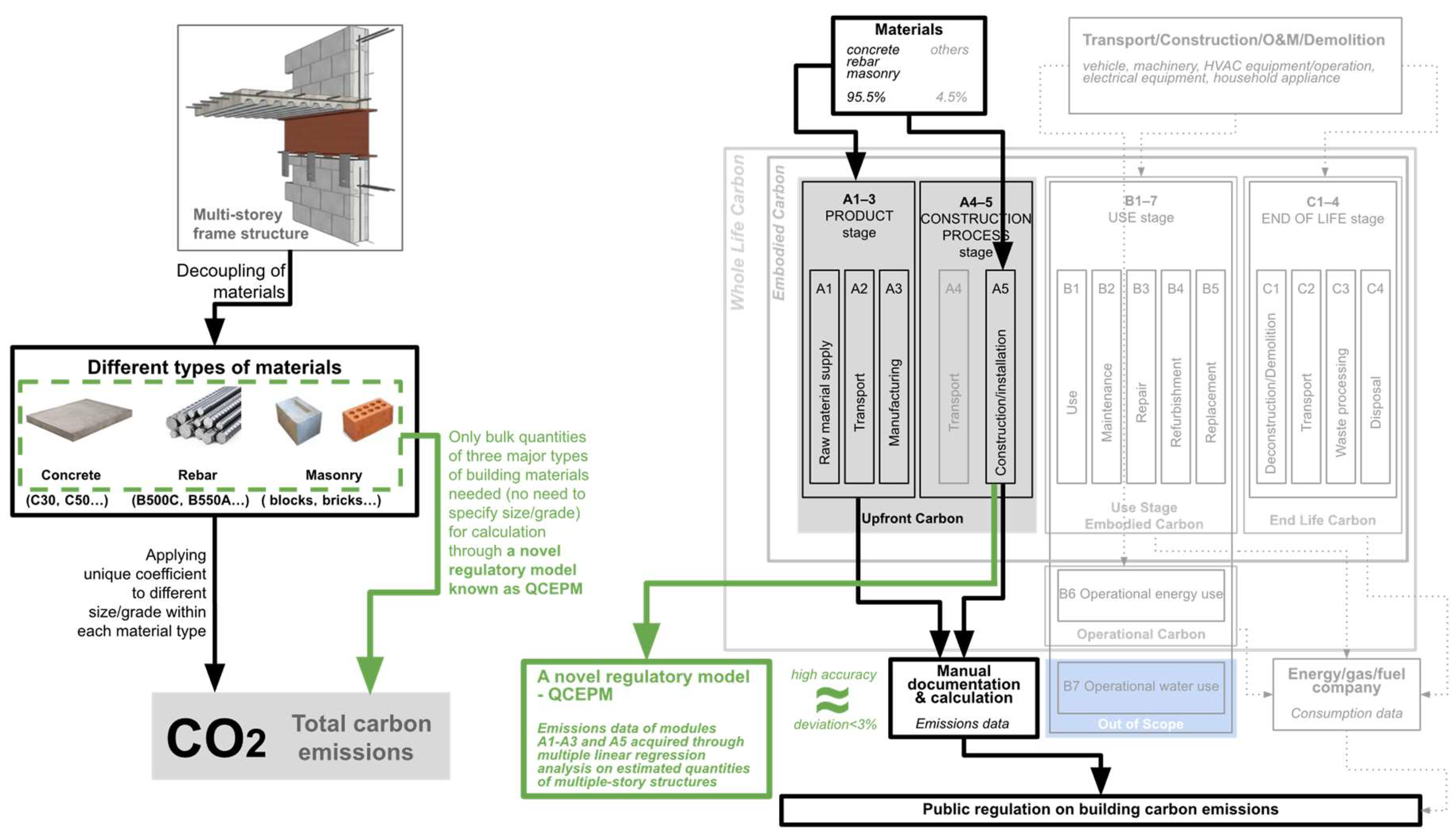
Figure 2.
Project timeline within Module A5 of building LCA.
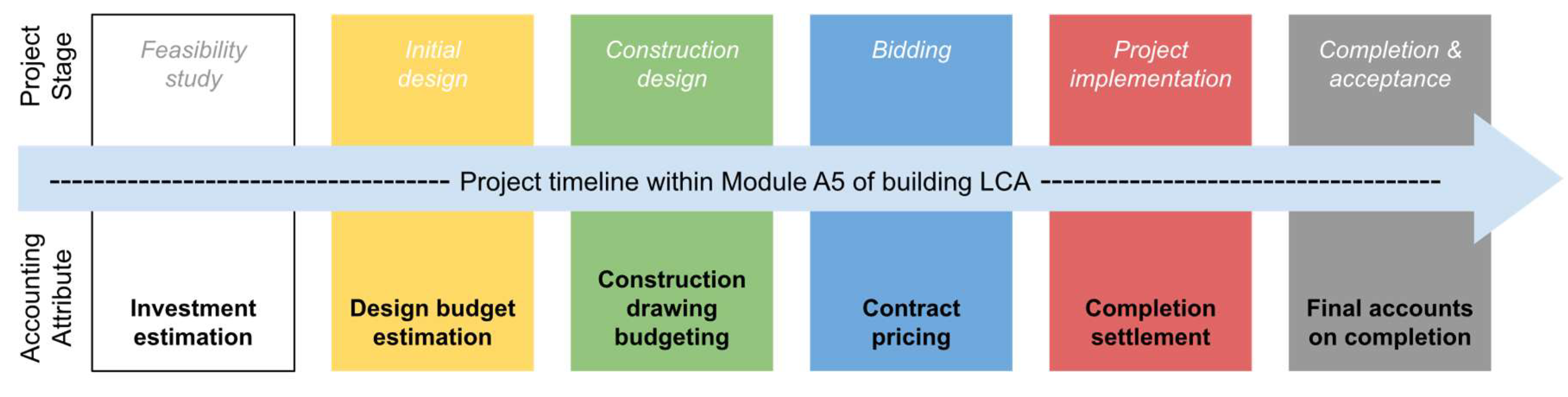
Figure 3.
Reference building.
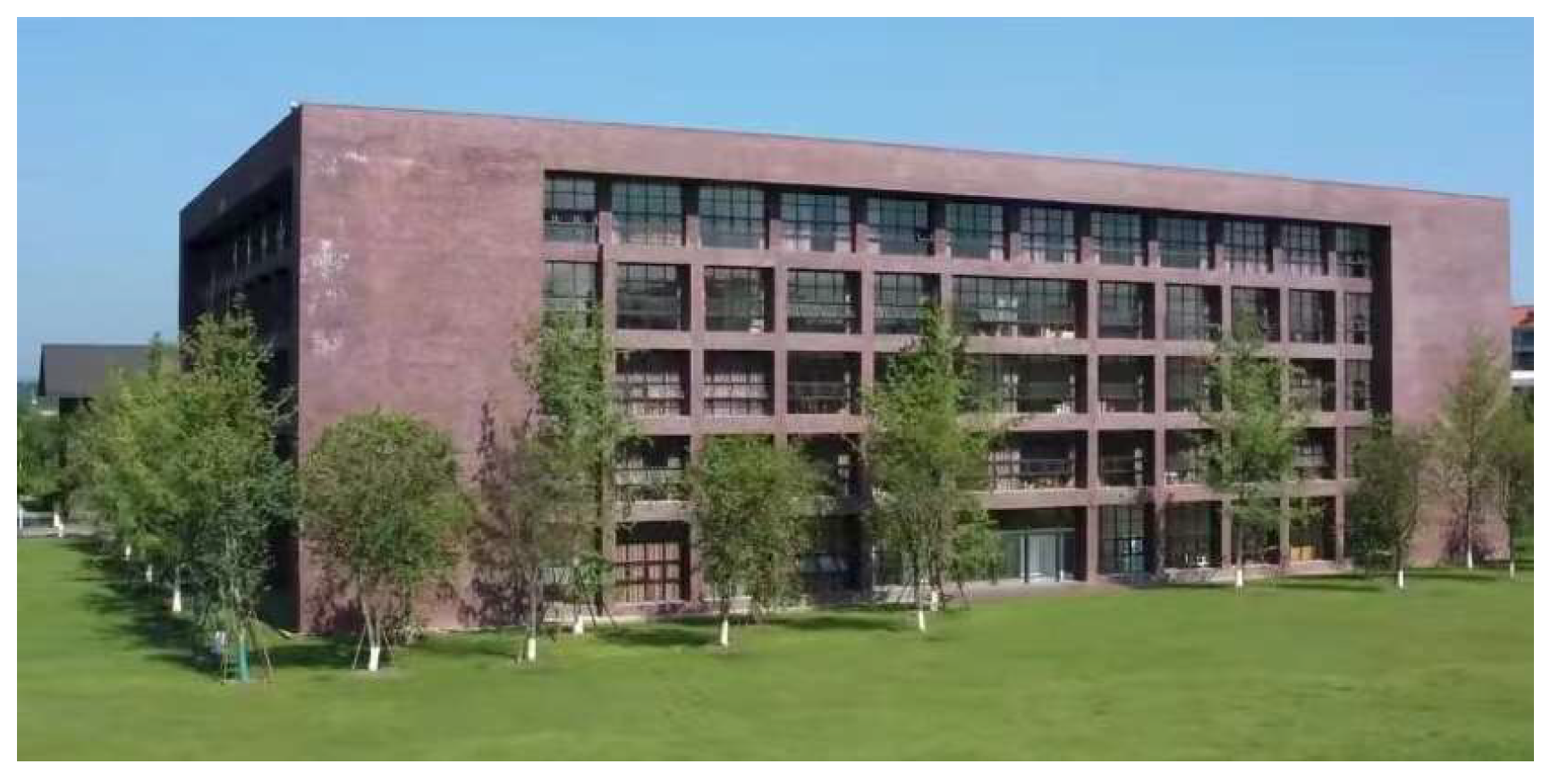
Figure 4.
Structural model of the reference building.
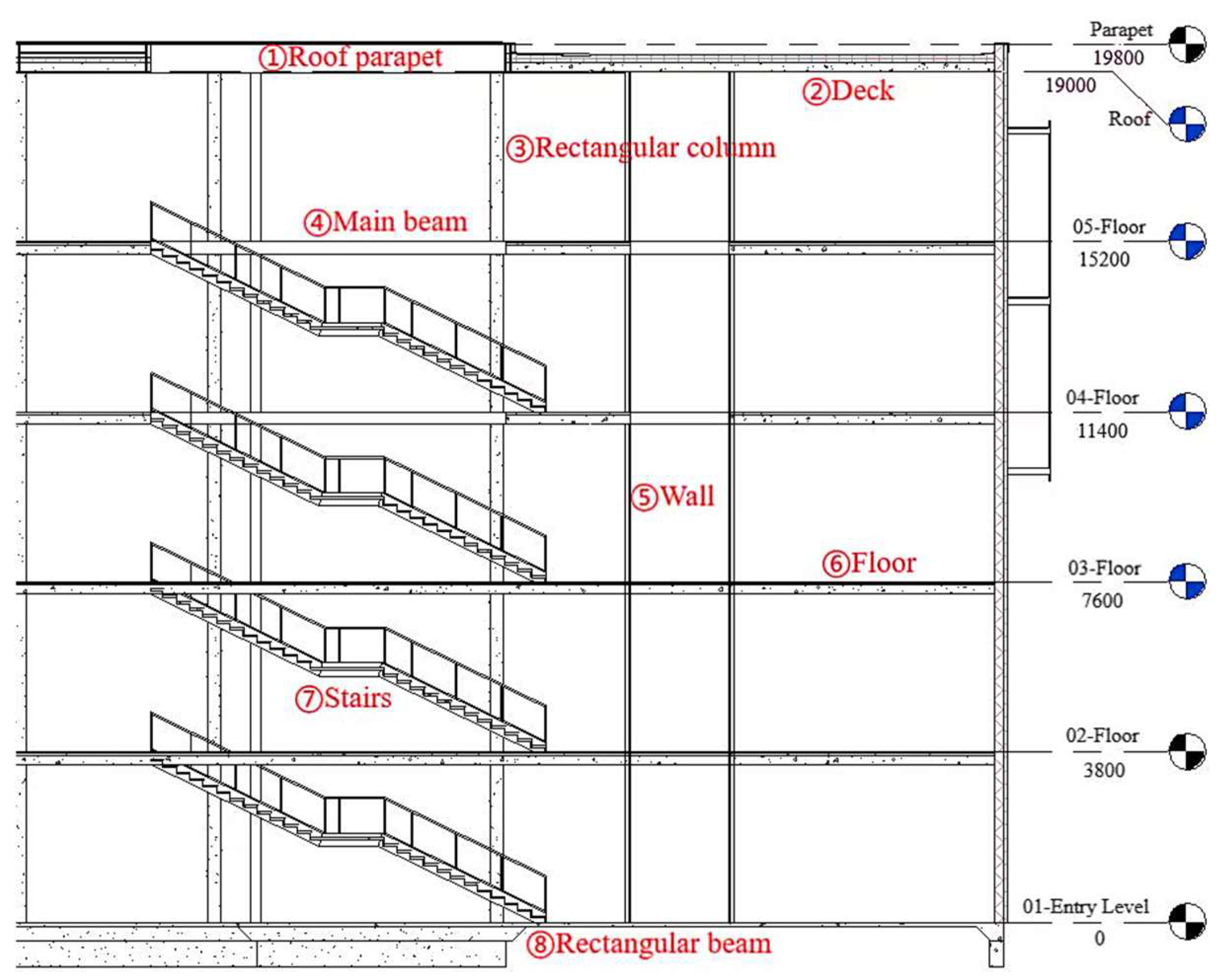
Figure 5.
Distribution of 20 data sets in terms of specific carbon emissions (kgCO2e/m2) and the percentage error (%) between their QCEPM-calculated and manually calculated results.
Figure 5.
Distribution of 20 data sets in terms of specific carbon emissions (kgCO2e/m2) and the percentage error (%) between their QCEPM-calculated and manually calculated results.
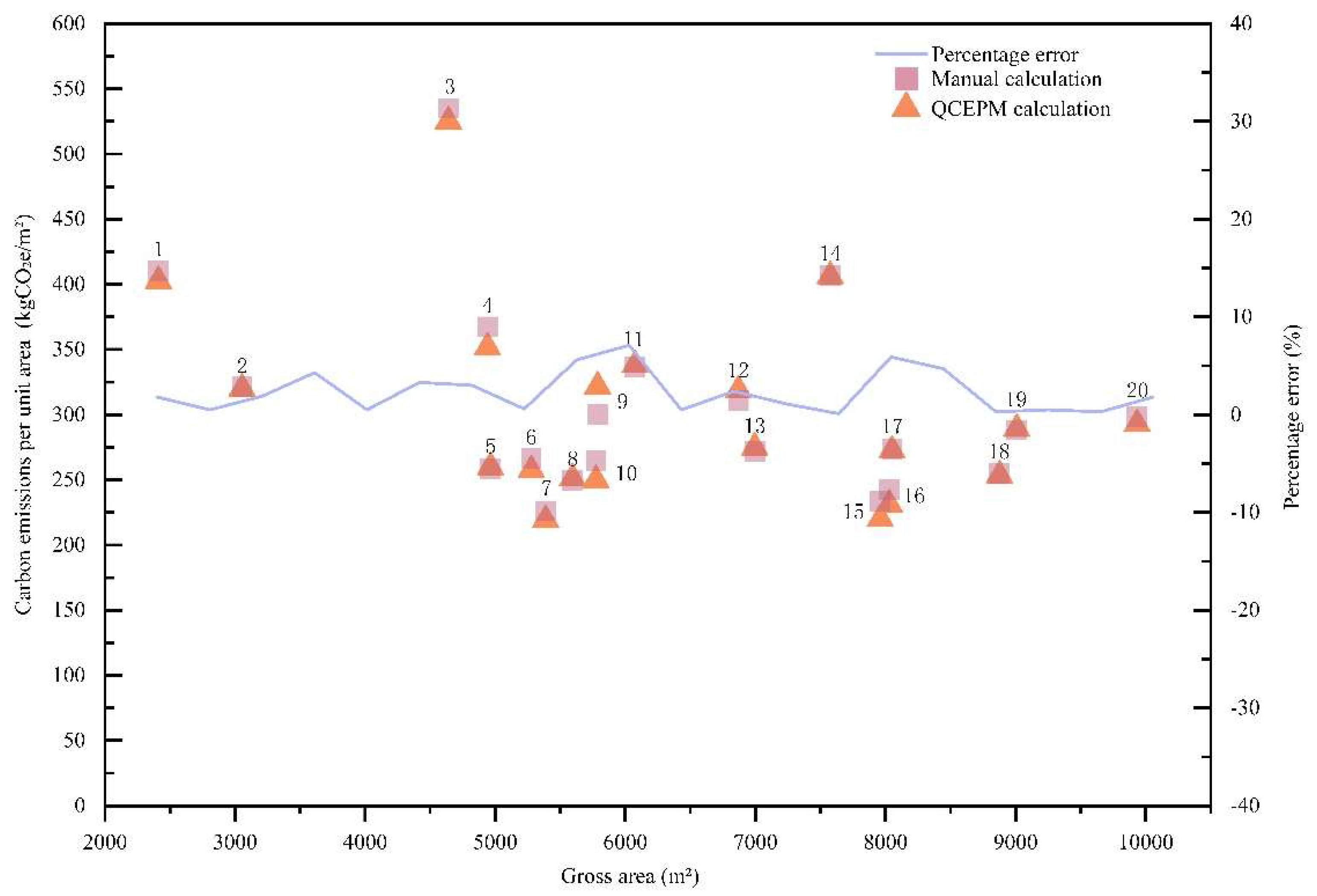
Figure 6.
Correlation between QCEPM-calculated and manually calculated CO2e values.
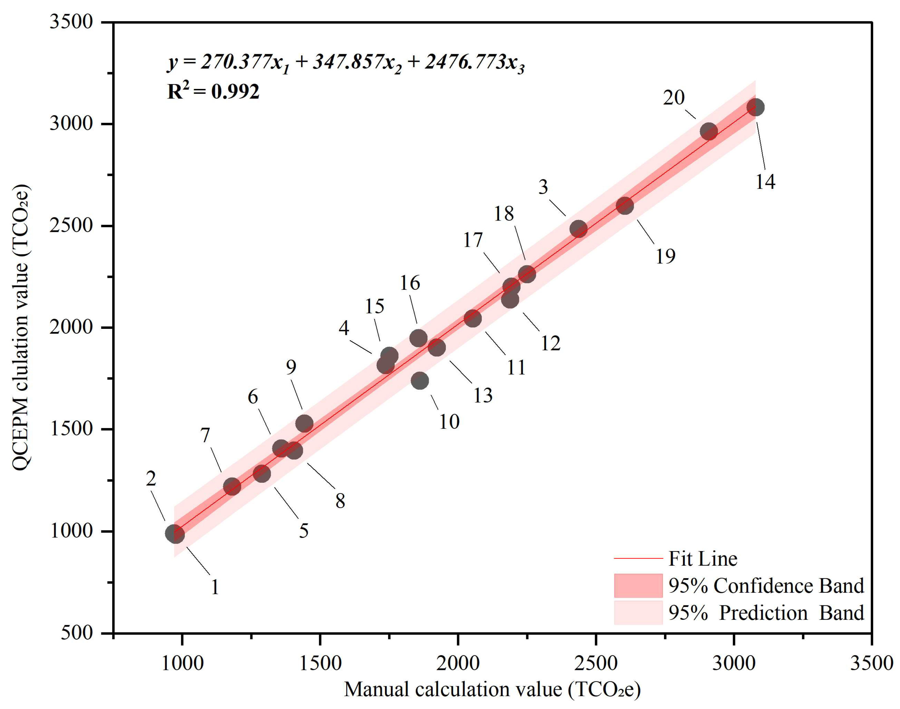
Figure 7.
Accumulative unit area error of 10 case study projects.
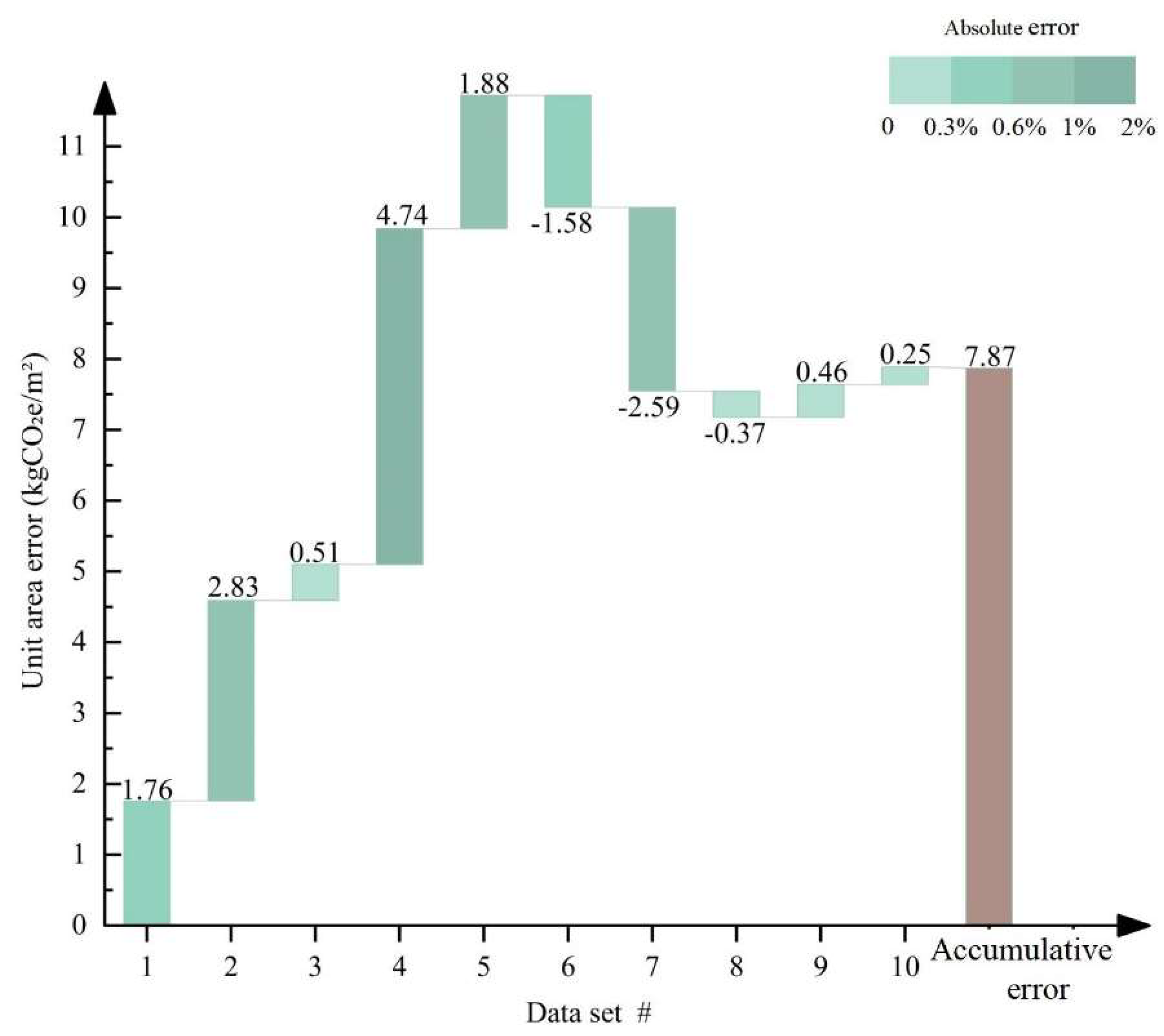

Table 1.
Comparison of three carbon emissions accounting methods.
| Method | Principles | Characteristics | Applicability |
|---|---|---|---|
| Real-time monitoring | Basic data measured from emissions sources are summarized into carbon emissions | High result accuracy, high data acquisition difficulty, high equipment investment | Narrow application scope, generally used for emissions in small regions with available monitoring data |
| Mass balance | Carbon emissions are obtained by subtracting the non-CO2 carbon output from the input carbon content | Can describe GHG production in great detail only if the intermediate reaction processes are clear, demands high data accuracy and large workload | Can be used to check the accuracy of calculations by other methods, mainly used for accounting emissions during the production process |
| Emission factor | Carbon emissions are obtained by multiplying the volume of production or consumption activities that result in greenhouse gas emissions with the coefficient corresponding to the activity volume data | Simple and easy to understand, with a large number of reliable data and application cases. However, emission factors vary from region to region, leading to uncertainty when the emission system changes | Suitable for carbon emission calculations when the internal complexity of emission sources is low |
Table 2.
Major building materials and their emission source.
| No | Building material | Emission source |
|---|---|---|
| 1 | Plastics (polyvinyl chloride, polyurethane, polypropylene, polycarbonate, ABS, nylon) | Petrochemical extraction and processing, energy-intensive production |
| 2 | Tiles | High-temperature firing during manufacturing, transportation |
| 3 | Clay | Energy use in extraction and processing |
| 4 | Gypsum | Energy use in extraction and processing |
| 5 | Stone (granite, marble, sandstone, slate) | Energy use in extraction and transportation |
| 6 | Metal (aluminum, stainless steel, copper and titanium) | Energy-intensive extraction and processing |
| 7 | Timber | Deforestation, transportation, processing |
| 8 | Masonry | Energy-intensive firing, transportation |
| 9 | Gravel | Energy use in extraction and transportation |
| 10 | Sand | Energy use in extraction and transportation |
| 11 | Rebar (including steel) | Energy-intensive steel production process |
| 12 | Concrete (including mortar) | Cement production, energy-intensive manufacturing process |
Table 3.
Distribution of selected data.
| Data set # | Building classification | City | Structure type | No. of floors | Gross area(m2) | Year |
|---|---|---|---|---|---|---|
| 1 | School | Chengdu | Framing | 5 | 2411.92 | 2015 |
| 2 | School | Chengdu | Framing | 5 | 3054.08 | 2018 |
| 3 | School | Chengdu | Framing | 4 | 4640.73 | 2020 |
| 4 | Multi-Family Home | Chengdu | Framing | 5 | 4940.44 | 2017 |
| 5 | Multi-Family Home | Chengdu | Framing | 5 | 4964.08 | 2018 |
| 6 | Multi-Family Home | Chengdu | Framing | 5 | 5277.91 | 2020 |
| 7 | Apartment building | Chengdu | Framing | 6 | 5387.06 | 2023 |
| 8 | Apartment building | Chengdu | Shear wall framing | 7 | 5594.79 | 2023 |
| 9 | Apartment building | Chengdu | Framing | 4 | 5775.11 | 2019 |
| 10 | Apartment building | Chengdu | Framing | 3 | 5786.97 | 2022 |
| 11 | Apartment building | Chengdu | Framing | 5 | 6075.29 | 2022 |
| 12 | Hospital | Bazhong | Shear wall framing | 4 | 6869.34 | 2019 |
| 13 | Office building | Luzhou | Shear wall framing | 6 | 6995.58 | 2018 |
| 14 | Apartment building | Chengdu | Framing | 7 | 7575.78 | 2016 |
| 15 | Hotel/Motel | Chengdu | Framing | 5 | 7960.50 | 2021 |
| 16 | College | Chengdu | Framing | 5 | 8029.49 | 2019 |
| 17 | School | Chengdu | Framing | 5 | 8051.75 | 2021 |
| 18 | Retail and Service | Chengdu | Framing | 6 | 8876.40 | 2019 |
| 19 | Retail and Service | Chengdu | Framing | 6 | 9009.63 | 2023 |
| 20 | Recreational Facility | Chengdu | Framing | 6 | 9934.70 | 2023 |
Table 4.
Page 1 in the detailed quantity list of data set #16.
| No. | Item code | Item name | Item Features | Unit | Quantity | Cost (¥) | ||
| Unit price | Subtotal | Labor cost | ||||||
| 10 | 010401003001 | Solid brick wall |
1.Block type: aerated concrete block 2.Wall type: interior wall3.Motar strength grade: M54.Wall thickness: 120mm |
m3 | 12.36 | 322.24 | 3982.89 | 1198.12 |
| Masonry project cost subtotal | 461858.24 | 143531.11 | ||||||
| Concrete and Reinforcement Works | ||||||||
| 11 | 010501001001 | Bedding | 1.Concrete type: commercial concrete 2.Concrete Strength Grade:C15 |
m3 | 85.72 | 362.3 | 31056.36 | 1911.98 |
| 12 | 010501002001 | Strip foundation | 1.Concrete type: commercial concrete 2.Concrete Strength Grade:C30 |
m3 | 21.45 | 402.65 | 8636.84 | 500.32 |
| 13 | 010501003001 | Independent foundation | 1.Concrete type: commercial concrete 2.Concrete Strength Grade:C30 |
m3 | 347.86 | 402.65 | 140065.83 | 8113.83 |
| 14 | 010502001001 | Rectangular column | 1.Concrete type: commercial concrete 2.Concrete Strength Grade:C25 |
m3 | 184.17 | 389.87 | 71802.36 | 5027.84 |
| 15 | 010502001002 | Rectangular column | 1.Concrete type: commercial concrete 2.Concrete Strength Grade:C30 |
m3 | 139.67 | 409.97 | 57260.51 | 3812.99 |
| 16 | 010502002001 | Structural column | 1.Concrete type: commercial concrete 2.Concrete Strength Grade:C25 |
m3 | 71.01 | 389.87 | 27684.67 | 1938.57 |
| 17 | 010502002002 | Structural column | 1.Concrete type: commercial concrete 2.Concrete Strength Grade:C30 |
m3 | 16.02 | 409.97 | 6567.72 | 437.35 |
| 18 | 010503002001 | Rectangular beam | 1.Concrete type: commercial concrete 2.Concrete Strength Grade:C25 |
m3 | 75.44 | 389.37 | 29374.07 | 2013.12 |
| 19 | 010503002002 | Rectangular beam | 1.Concrete type: commercial concrete 2.Concrete Strength Grade:C30 |
m3 | 13.5 | 409.47 | 5527.85 | 360.25 |
| Subtotal for this page | 377976.21 | 24116.25 | ||||||
Table 5.
Processed results from data set #16.
| No. | Material name | Unit | Quantity | Carbon emission factor (kgCO₂e/unit) | Carbon emissions (kgCO₂e) | |
|---|---|---|---|---|---|---|
| 1 | Concrete (C15) | m3 | 85.72 | 228 | 19544.16 | |
| 2 | Concrete (C20) | m3 | 1772.20 | 263 | 466088.60 | |
| 3 | Concrete (C30) | m3 | 912.39 | 248 | 226272.72 | |
| 4 | Gravel Concrete | m3 | 217.86 | 295 | 64268.70 | |
| Concrete project subtotal | 2988.17 | — | 776174.18 | |||
| 5 | Rebar (HPB300) | t | 41.21 | 2310 | 95188.17 | |
| 6 | Rebar (HRB335) | t | 6.09 | 2340 | 14248.26 | |
| 7 | Rebar (HRB400) | t | 216.50 | 2350 | 508784.40 | |
| Rebar project subtotal | 263.80 | — | 618220.83 | |||
| 8 | Solid brick | m3 | 60.17 | 341 | 20517.97 | |
| 9 | Porous brick | m3 | 445.95 | 341 | 152068.95 | |
| 10 | Building blocks | m3 | 885.68 | 327 | 289617.36 | |
| Masonry project subtotal | 1391.80 | — | 462204.28 | |||
| Grand total | — | — | 1856599.29 | |||
Table 6.
Process carbon emissions data (in ascending order of gross area).
| Data set# | Quantity | Carbon emissions (kgCO₂e) | Gross area (m2) | Carbon emissions/unit area (kgCO₂e/m2) | ||
| Concrete (m³) | Rebar (t) | Masonry (m³) | ||||
| 1 | 1618.60 | 138.43 | 597.43 | 971114.28 | 2411.92 | 402.63 |
| 2 | 1259.19 | 168.43 | 643.17 | 977463.40 | 3054.08 | 320.05 |
| 3 | 2028.72 | 228.79 | 3925.88 | 2436649.78 | 4640.73 | 525.06 |
| 4 | 3797.81 | 187.73 | 918.32 | 1737206.39 | 4940.44 | 351.63 |
| 5 | 1897.44 | 168.73 | 1006.18 | 1289469.01 | 4964.08 | 259.76 |
| 6 | 2089.77 | 158.16 | 1285.66 | 1359164.66 | 5277.91 | 257.52 |
| 7 | 609.90 | 260.84 | 1172.56 | 1181110.56 | 5387.06 | 219.25 |
| 8 | 2192.10 | 214.19 | 780.68 | 1405111.38 | 5594.79 | 251.15 |
| 9 | 1715.64 | 211.94 | 1545.25 | 1442744.98 | 5775.11 | 249.82 |
| 10 | 2291.90 | 256.95 | 1384.37 | 1862171.38 | 5787.97 | 321.79 |
| 11 | 3026.36 | 294.37 | 1420.99 | 2053804.75 | 6075.29 | 338.06 |
| 12 | 3417.75 | 236.94 | 1790.69 | 2189107.89 | 6869.34 | 318.68 |
| 13 | 2756.31 | 230.94 | 1672.39 | 1923116.79 | 6995.58 | 274.90 |
| 14 | 3479.03 | 580.38 | 2020.19 | 3078582.56 | 7575.78 | 406.37 |
| 15 | 2560.02 | 295.90 | 1248.16 | 1768854.13 | 7960.50 | 222.20 |
| 16 | 2988.17 | 263.80 | 1391.80 | 1856599.36 | 8029.49 | 231.22 |
| 17 | 2735.34 | 412.73 | 1259.19 | 2194156.84 | 8051.75 | 272.51 |
| 18 | 2459.30 | 340.31 | 2161.22 | 2249875.76 | 8876.40 | 253.48 |
| 19 | 3266.15 | 447.05 | 1740.60 | 2604957.50 | 9009.63 | 289.13 |
| 20 | 3942.87 | 607.96 | 1123.67 | 2909373.28 | 9934.70 | 292.85 |
Table 7.
Collinearity analysis results.
| Collinearity statistics | ||
| Capacity | VIF | |
| Concrete | 0.657 | 1.522 |
| Rebar | 0.642 | 1.557 |
| Masonry | 0.963 | 1.039 |
Table 8.
Analysis of variance results.
| Sum of squares | Degrees of freedom | Mean square | F-Value | Significance | |
|---|---|---|---|---|---|
| Between | 6842727600158.907 | 3 | 2280909200052.969 | 666.835 | 0.000 |
| Within | 54728000956.385 | 16 | 3420500059.774 | — | — |
| Total | 6897455601115.293 | 19 | — | — | — |
Table 9.
Regression and T-test.
| Unstandardized Coefficients | Standardized coefficients Beta |
t | Significance | ||
| B | Standard error (σ) | ||||
| (Constant) | -18040.215 | 7026.180 | — | -0.384 | 0.706 |
| Concrete | 271.499 | 19.154 | 0.389 | 14.175 | <0.001 |
| Rebar | 2470.192 | 126.637 | 0.542 | 19.506 | <0.001 |
| Masonry | 348.319 | 19.021 | 0.416 | 18.312 | <0.001 |
Table 10.
Model fit degree and Durbin Watson test.
| Model | R | R² | Adjusted R square | Std. error of the estimate | Durbin-Watson |
| 1 | 0.996 | 0.992 | 0.991 | 58485.04133 | 1.939 |
Table 11.
Error analysis between QCEPM calculation and manual calculation.
| Data Set # | Manual calculation (kgCO₂e) | QCEPM calculation (kgCO₂e) | Error (%) |
| 1 | 971114.28 | 989493.1801 | 1.89 |
| 2 | 977463.40 | 981951.5956 | 0.46 |
| 3 | 2436649.78 | 2483409.275 | 1.92 |
| 4 | 1737206.39 | 1814699.065 | 4.46 |
| 5 | 1289469.01 | 1282420.17 | -0.55 |
| 6 | 1359164.66 | 1405875.837 | 3.44 |
| 7 | 1181110.56 | 1218337.048 | 3.15 |
| 8 | 1405111.38 | 1396169.059 | -0.64 |
| 9 | 1442744.98 | 1527567.243 | 5.88 |
| 10 | 1862171.38 | 1739166.767 | -6.61 |
| 11 | 2053804.75 | 2043761.948 | -0.49 |
| 12 | 2189107.89 | 2136934.35 | -2.38 |
| 13 | 1923116.79 | 1901326.762 | -1.13 |
| 14 | 3078582.56 | 3081873.76 | 0.11 |
| 15 | 1768854.13 | 1860730.526 | 6.22 |
| 16 | 1856599.36 | 1947712.201 | 4.91 |
| 17 | 2194156.84 | 2200764.22 | 0.30 |
| 18 | 2249875.76 | 2261122.519 | 0.50 |
| 19 | 2604957.50 | 2597339.844 | -0.29 |
| 20 | 2909373.28 | 2963658.801 | 1.87 |
Table 12.
Case project information.
| Data set # | Project name | City | Structure type | Gross area (m2) | No. of floors | Year |
| 1 | Jinjiang Commercial Building | Chengdu | Framing | 1861.31 | 2 | 2023 |
| 2 | Longjianglu Elementary School building | Chengdu | Framing | 3002.10 | 6 | 2023 |
| 3 | Jinxiu Residence | Chengdu | Framing | 4940.44 | 6 | 2023 |
| 4 | Banan Middle School building | Chongqing | Framing | 5277.91 | 5 | 2023 |
| 5 | Liangchen Residence | Chengdu | Framing | 5648.51 | 3 | 2022 |
| 6 | Zuoyu Residence | Chengdu | Framing | 8315.25 | 6 | 2023 |
| 7 | Rilian Residence | Chengdu | Framing | 8798.40 | 6 | 2023 |
| 8 | Xiayu Residence | Chengdu | Framing | 10264.80 | 7 | 2023 |
| 9 | Aochuang Commercial Complex | Chengdu | Shear wall framing | 13645.65 | 5 | 2022 |
| 10 | Tianchen Office Tower | Chengdu | Framing | 18109.90 | 6 | 2023 |
Table 13.
Case study results (in ascending order of project gross area).
| Data set # |
Quantity | Manual calculation (kgCO₂e) |
QCEPM calculation (kgCO₂e) | Error (%) | Unit area error (kgCO₂e/m2) |
||
| Concrete (m³) | Rebar (t) | Masonry (m³) | |||||
| 1 | 716.42 | 98.11 | 600.42 | 642724.42 | 645995.54 | 0.51 | 1.76 |
| 2 | 1421.71 | 156.53 | 1106.59 | 1149602.60 | 1158098.32 | 0.74 | 2.83 |
| 3 | 2756.98 | 160.13 | 1104.71 | 1526345.96 | 1528860.64 | 0.16 | 0.51 |
| 4 | 1408.81 | 177.65 | 1121.72 | 1186995.56 | 1212036.50 | 2.11 | 4.74 |
| 5 | 2233.84 | 261.11 | 1097.11 | 1622969.47 | 1633621.42 | 0.66 | 1.86 |
| 6 | 2657.55 | 268.99 | 2318.96 | 2206884.00 | 2193716.94 | -0.60 | -1.58 |
| 7 | 3291.52 | 353.76 | 2425.03 | 2634963.66 | 2612183.54 | -0.86 | -2.59 |
| 8 | 2708.1 | 386.91 | 2739.7 | 2649052.36 | 2645277.99 | -0.14 | -0.37 |
| 9 | 4518.09 | 769.52 | 1405.15 | 3610613.97 | 3616959.51 | 0.18 | 0.46 |
| 10 | 4565.1 | 665.99 | 3741.03 | 4183085.05 | 4187615.08 | 0.11 | 0.25 |
Disclaimer/Publisher’s Note: The statements, opinions and data contained in all publications are solely those of the individual author(s) and contributor(s) and not of MDPI and/or the editor(s). MDPI and/or the editor(s) disclaim responsibility for any injury to people or property resulting from any ideas, methods, instructions or products referred to in the content. |
© 2024 by the authors. Licensee MDPI, Basel, Switzerland. This article is an open access article distributed under the terms and conditions of the Creative Commons Attribution (CC BY) license (http://creativecommons.org/licenses/by/4.0/).
Copyright: This open access article is published under a Creative Commons CC BY 4.0 license, which permit the free download, distribution, and reuse, provided that the author and preprint are cited in any reuse.


