
Submitted:
29 May 2024
Posted:
29 May 2024
You are already at the latest version
Abstract
Elbow dislocation and instability present significant clinical challenges, necessitating a thorough understanding of the underlying bio-mechanical mechanisms. In this study, a quasi-static three-dimensional finite element model of the human elbow joint is developed to investigate stress distribution and stages of dislocation in the human elbow under various loading conditions. The model simulates the elbow joint in different degrees of flexion (30°, 45°, 60°, and 90°) and forearm positions (pronation and supination), providing detailed insights into the progression of dislocation. Significant findings include the identification of high stress concentrations on the humerus at 90° flexion and on the radial and coronoid processes at 30°, 45°, and 60° flexion. Three reproducible stages of dislocation were observed, particularly in flexed positions with forearm pronation or supination. These stages align with experimental observations and highlight the initial occurrence of bony failures, such as radial head and ulnar coronoid fractures, preceding soft tissue tears. Clinically, the study underscores that early-stage low-impact posterior elbow dislocations retain enough stability to be managed with closed reduction and early mobilization. However, as dislocations progress, significant damage to the medial and lateral collateral ligaments is expected, necessitating more invasive treatments. This research provides valuable bio-mechanical insights into elbow dislocation, aiding in the development of improved treatment strategies and enhancing patient outcomes through precise and timely clinical interventions. The validated FEM serves as a powerful tool for pre-surgical planning offering a comprehensive understanding of elbow joint mechanics.
Keywords:
Finite Element Modeling
; Elbow Dislocation
; MRI
; CT Scan
; Simpleware ScanIP
; bio-mechanics
; Ansys
; sport injury
1. Introduction
The elbow is a joint connecting the upper and lower arms humerus and radius and ulna parts, with a complex structure that is supported by soft tissues [2]. It comprises three separate joints: ulnohumeral where movement between the ulna and the proximal humerus occurs, radiohumeral where movement between the radius and the humerus occurs and superior radioulnar where movement between the radius and the ulna occurs. Ligaments form the joint capsule, hold the bones together and play an important role in maintaining the elbow stability and preventing dislocations. Four main ligaments exist: the ulnar collateral ligament, the radial collateral ligament, the annular ligament and the quadrate ligament. Figure 1 shows different parts involved in the elbow: ulna, radius, humerus, capsules, bundles and ligaments. The elbow allows motions controlled by the contraction (flexion) and relaxation (extension) of muscles, and its range of motion is related to age, sex and body mass index [3]. The musculotendinous units overlying the ulnar collateral ligament play an important role in maintaining the dynamic valgus stability of the elbow [4]. Other elements like bone surfaces, capsule and muscles affect the elbow’s range of motion and have stabilizing effects.
Among other joints, the elbow is the most frequently dislocated in children and the second most frequently dislocated in adults, after the shoulder [5]. Elbow injuries can be seen in sports [4,6,7] and other accidents like falls from heights [8], and traffic and machine accidents [9]. Elbow dislocations can affect the hand’s motion and functionality and result from injury mechanisms associated to high energy impacts like falling onto an outstretched hand [10]. Another known mechanism for elbow dislocation is hyperextention force with the forearm supinated [11,12]. They can be simple without fracture or complex with fractures and their treatment may require surgical intervention [5]. Additionally, they can be classified according to their directions as they can be posterior, lateral, medial, posterolateral, posteromedial or divergent. In elbow dislocation, any of the bone surfaces, ligaments, capsule and muscles can be injured. For the treatment of elbow dislocations, it is not enough to understand the anatomy and the interactions between the bony articulations. Recognizing the precise injury pattern is critical as it helps to restore the functionality and to prevent chronic instability at the elbow [13].
This study aims to improve the understanding of elbow dislocation mechanics and stages. This is a challenging problem in biomechanics and many models attempted to solve it by focusing on inverse dynamics using mathematical models to determine muscles forces [14]. The current approach is to establish finite element models of the different parts of the elbow with a high fidelity that allows realistic and precise simulations of different scenarios and underlying conditions. The approach adopted in this study follows the following steps:
- Establishing FE models for a human elbow using CT scans and considering contacts and properties of the different parts.
- Modeling different elbow configurations and loading conditions.
- Studying analysis results in conjunction with experimental results obtained from a separate study made with cadaver elbows and reported in [1].
The rest of the paper is organized as follows: Section 2 shows previous work in finite element modeling of human elbows. Section 3 shows the process followed in this study to establish finite element models of elbows, with boundary conditions and contacts developed in Section 4. Results are shown and discussed in Section 5 and a conclusion ends the paper.
2. Finite Element Analysis and Elbow Models
Finite element analysis (FEA) of structural stresses was seen in orthopedics since 1972 [15]. In this area, applications of finite element stress analysis covered bones, bone-prosthesis structures, fracture fixation devices and tissues [15]. Since then, the development of computing devices and the increase in their performances has positively affected the usage of FEA in orthopaedic bio-mechanics [16,17]. Indeed, FEA can be seen in different parts of the human body [18,19,20,21,22] and in several applications related to orthopedics, like implant design [23], alloys for fractures and tissues rehabilitation design [24], and other aspects of orthopedic and trauma surgery [25]. Previous work on finite element analysis of the elbow joint had different objectives. Mainly, while some studies addressed fractures and dislocations, others addressed the behavior of different elements under load. Also, other aspects were addressed in FEA like elbow prostheses.
In [26], MRI results were used to construct a finite element model for the cartilage and ligaments, which allowed to simulate different conditions for the annular ligament. Different buckling angles and muscle strengths were simulated. The used software were Solid Works and ABAQUS and the analysis addressed the load, contact area and stress, as well as the MCL stress. The authors concluded the necessity of reconstructing a ruptured annular ligament for the avoidance of clinical symptoms related to MCL and annular ligament cartilage stresses.In [27], the humerus, ulna and radius were modeled along with other parts of the elbow and finite element analysis was performed taking into account mechanical properties of the biological tissues. A load was simulated to be applied on the distal part of the ulna-radius, as if an individual were standing on their hands. Results showed areas prone to injury, as well as the presence of stress concentrations especially in the ligament-bone relation areas. The study shown in [28] relied on finite element analysis and aimed to reach a methodology allowing to predict the behavior of elbow-related muscles under load and during joint movements. To simplify the analysis, a 1D rod element was used instead of 3D hexahedral and tetrahedral elements. Reconstruction of the joints done using NMR images. In [29], medical images were used to model a human elbow and study the stresses in the elbow during heavy weight lifting. Finite element analysis was used and was shown to allow the prediction of stress level and displacement in bones, and thus the safe load that can be carried without causing bone injuries.
Finite element models of 8 human cadaver elbows were developed in [30] based on their CT scans. The study also subjected the actual elbows to loads and compared the resulting pressure distributions, stiffness’s and peak pressures with those obtained in the model. Reported results showed correlations between the two. Another study was made in [31] where the treatment of ulna-coronoid process basal fracture with single and double screws was investigated. CT scans from 63 adult volunteers allowed to reconstruct and measure properties for the ulna and coronoid. Models of basal fractures were developed and a finite element study was made and allowed to conclude that single or double screw fixations are stable when pull-out and rotational stability factors are in reasonable conditions.In another work [32], the bio-mechanical analysis of the elbow dislocation by a compressive force mechanism was studied. This work included a finite element analysis where CT-scan of a 32 year old male was mapped into a 2D finite element model. The model consisted of the cortical, cancellous and subchondral bones, and the cartilage. Material properties were assumed linear and isotropic. Axial loads were applied as elbow joint changed from 15º hyper-extension and 0º, 30º, 60º and 90º in flexion.
Regarding prostheses in elbows, a study was made in [33] where FEA was relied on to analyze stresses of total elbow arthroplasty and to identify areas where implant mobilization risks exist. Elbow prosthesis models were obtained using 3D scanning and computer-aided drafting and combined with their elastic properties, resistance and stresses in the analysis. It was found in the study that some variations in positioning in the sagittal plane can result in longer implant survival. In the same vein, the study presented in [34] investigated the mechanical behavior at the interface between the bone and the cement through FEA. It was shown that such a study can be used to provide guidelines for surgeons aiming to reduce the aseptic loosening through the implant configurations.
3. Materials and Methods
Transverse computed tomography (CT) scans of a 28-year-old healthy male human elbow participant were utilized to extract the 3D geometry of the humerus, ulna, and radius. The extraction process was facilitated by a specialized image processing software package called Simpleware ScanIP, a 3D image segmentation and processing Software1. Additionally, ligament geometry measurements were obtained from MRI images of the participant. The participant provided consent for the experiment by signing a consent form. The multi-layer spiral CT scans were further processed using Simpleware FE Module, an image-Based meshing Software for FEA2. This preprocessor transformed the scans into a finite element mesh, which was subsequently imported into the Finite Element Analysis (FEA) Software Ansys 3. The model was divided into three distinct areas based on the different material properties: cortical bone, cartilage, and ligaments. These material properties were assumed to be linearly elastic and isotropic, with numerical values sourced from literature [26,35,36,37]. The total number of elements utilized in the model was 66,672 tetrahedral elements. Contact elements specific to the elbow joint, along with boundary conditions derived from previous experimental data on posterior elbow dislocations [1], were incorporated to validate the model’s accuracy. Subsequently, the finite element (FE) model was employed to investigate the behavior of ligaments and cartilage under varying flexion and extension angles. This analysis aimed to provide insights into the mechanical response of these soft tissues within the elbow joint, contributing to a better understanding of joint bio-mechanics and potential implications for clinical applications. Explanations regarding the modeling procedure (see Figure 2) are provided in the following subsections.
3.1. Data Processing and Selection
Individual images from the CT scan and MRI data were imported into Simpleware ScanIP. The data files were formatted in DICOM (The Digital Imaging and Communications in Medicine) standard format. A single DICOM file contains both a header (includes patient information), scan type, image dimensions, and all of the three dimensional image data. Figure 3 shows a CT scan data of the elbow joint after it has been imported into Simpleware ScanIP. For optimization purposes, the imported data underwent a series of processing algorithms, including cropping, resampling, and segmentation see Figure 4. The imported data was cropped to retain only the necessary image objects within designated volume limits and memory usage constraints.The data was then resampled to a resolution of 2.5 mm × 2.5 mm × 2.5 mm. Resampling artificially increased the resolution by super sampling the data without modifying object sizes. This sampling rate directly impacted the number of elements generated in Simpleware FE module and served as the primary method of controlling mesh density. The resampling interpolation method employed a combination of linear and nearest neighbor techniques. Given the complexity of the model, an assisted segmentation tool utilizing threshold and region-growing algorithms were applied to develop masks for segmentation purposes.
3.2. 3D Elbow Model Generation
To create a 3D representation of the elbow bone, ligaments, and cartilage, they were first delineated against their surroundings. Boundaries were marked for the humerus, ulna, radius, and cartilage on each image. Cartilage was defined as the space between two surface bones that are close enough to be in contact with each other, such as the humerus-ulna and the radius-ulna. Subsequently, 3D models were generated from six masks, each representing a different anatomical structure. These models were color-coded as follows: red for humerus, green for radius, blue for ulna (see Figure 5), yellow for ulna-humerus cartilage (see Figure 6), pink for radius-humerus cartilage and orange for ligaments (see Figure 7). The next step after creating the segmented masks was to generate a 3D visualization of the elbow model (Figure 8). Generating Finite Element meshes with Simpleware FE module, requires exporting segmented data as a volume export.
3.2.1. 3D FE Elbow Model Mesh Generation
After constructing the 3D solid model, the next step involves creating a finite element (FE) mesh and exporting the data into Simpleware FE Module. This process relies on two essential tools: mesh refinement and pre-smoothing. The density and complexity of the mesh produced by Simpleware FE module are directly correlated with the number of pixels within a mask. Mesh refinement is instrumental in enhancing the accuracy of the FE model by adjusting the density and complexity of the mesh. This adjustment is directly correlated with the number of pixels within a mask. By identifying specific areas within the model that require higher mesh density for detailed analysis, mesh refinement ensures optimal representation of geometric features and structural complexities. This is achieved by setting a global base spacing and strategically placing spheres at locations where increased mesh density is needed. Pre-smoothing is another integral aspect of the meshing process, aimed at improving the overall smoothness of meshed objects while maintaining high-quality elements. This unique feature is applied prior to mesh generation and effectively minimizes irregularities in the mesh surface. Despite its impact on element quality being minimal, pre-smoothing significantly enhances the realism and accuracy of the final mesh. Figure 9 and Figure 10 show the difference of FE mesh with and without Pre-smoothing algorithm applied. These figures serve as invaluable tools for illustrating the effectiveness of pre-smoothing in refining the mesh surface and enhancing the overall quality of the FE model.
3.2.2. Pre-Smoothing Process
In Simpleware FE module, the image data segmented in Simpleware ScanIP is transformed into a solid meshed model. The initial model is generated as a mesh of the entire image volume using “brick” (voxel) elements. Each mask created in Simpleware ScanIP is reproduced within the meshed volume as a separate part and is displayed in the same color as the mask in Simpleware ScanIP. Any mesh elements that are not represented in a mask are assigned to an additional background part that is colored grey and is initially invisible.
3.2.3. The Stages of the Mesh Process
The mesh process follows the consecutive stages below:
- Import
- Voxel meshing
- Surface mesh smoothing
- Surface mesh optimization
- Reduction of surface mesh tetrahedral
- Adaptive meshing
By applying a smoothed mesh approach, the aim is to mitigate irregularities and improve the surface continuity of the meshed elements. This process helps to achieve a more uniform distribution of nodes and elements throughout the model, resulting in smoother transitions between adjacent elements. Mesh quality, also known as tetrahedral quality, is a crucial aspect during optimization. The reduction of tetrahedral number directly influences the quality of resulting hexahedra. A minimum quality target of 0.15 is set for the mesh elements. This quality threshold serves as a benchmark to ensure that the mesh meets certain standards of element quality and integrity. The surface mesh option is utilized to establish criteria for adding extra smoothness to parts on the surfaces and to determine quality improvement criteria for surface mesh elements.
In most cases, the optimizer effectively generates meshes with high quality while maintaining surface smoothness and topology. Surface smoothing tends to decrease the volume of a part and may also reduce the quality of surface mesh elements, but these issues can be rectified during optimization. Adaptive meshing is employed to decrease the number of mesh nodes and elements. This process involves re-meshing the non-surface interior mesh into larger voxel (brick) elements. By doing so, mesh density at the surface part—typically the region of interest—is preserved, while reducing mesh density in the part volume.
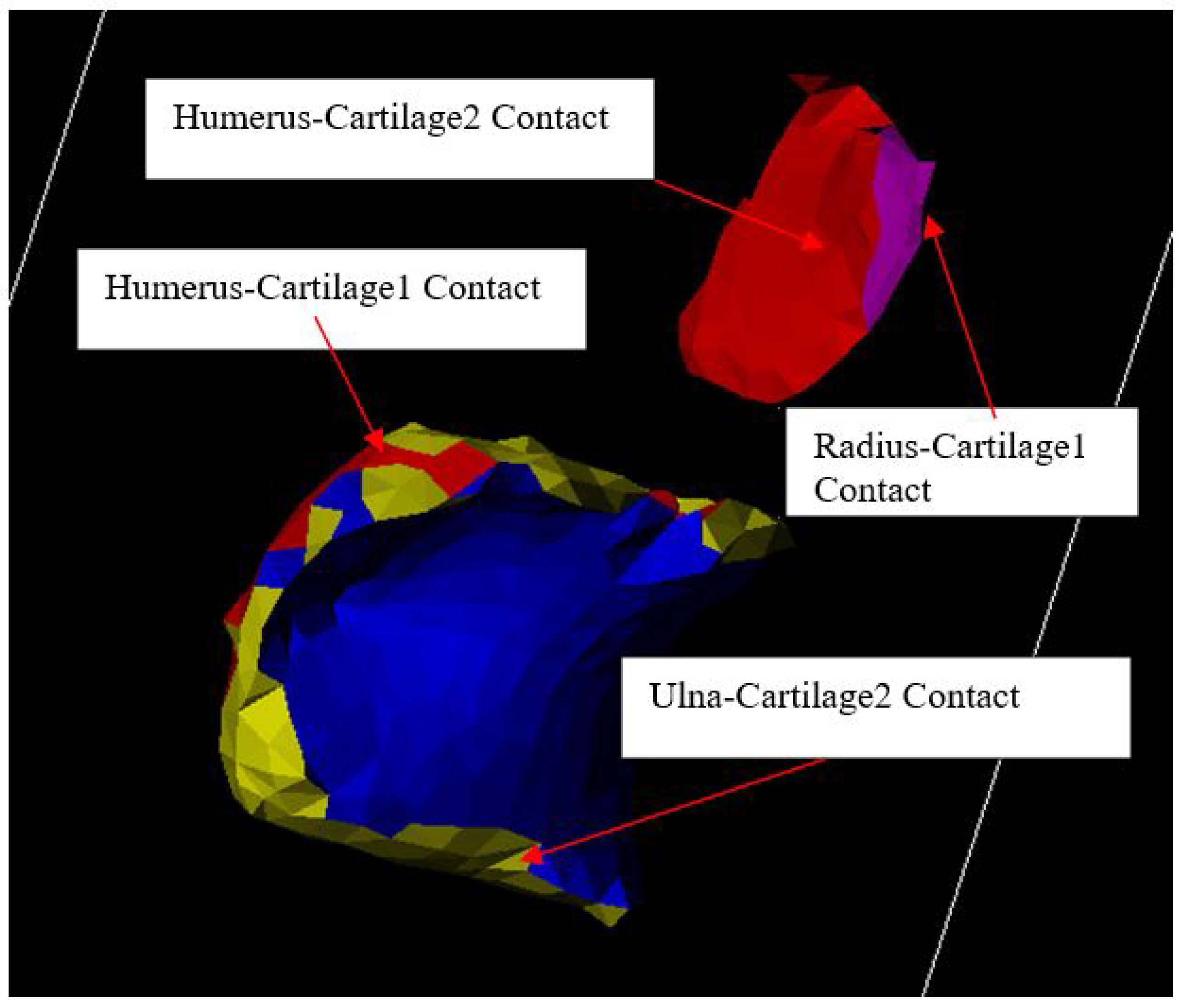
3.2.4. Contacts Formation
A contact is characterized as a surface comprising solely the exterior faces of a specified part, directly interacting with the exterior faces of another specified part. Consequently, a contact inherently exhibits uni-directional, signifying that it always represents a single-sided surface. It is defined by the two parts involved, designated as "from" and "to" parts, with the contact consistently belonging to the "from" part. Below is list of defined contacts generated in the established elbow joint model.
- Ulna surface in contact to Cartilage1
- Cartilage1 surface in contact to Humerus surface
- Radius surface in contact to Cartilage2
- Cartilage2 surface in contact to Humerus surface
- Ligament surface in contact to Ulna surface
- Ligament surface in contact to Humerus surface
- Ligament surface in contact to Radius surface
Figure 11.
Ligament contacts with ulna, radius and humerus.
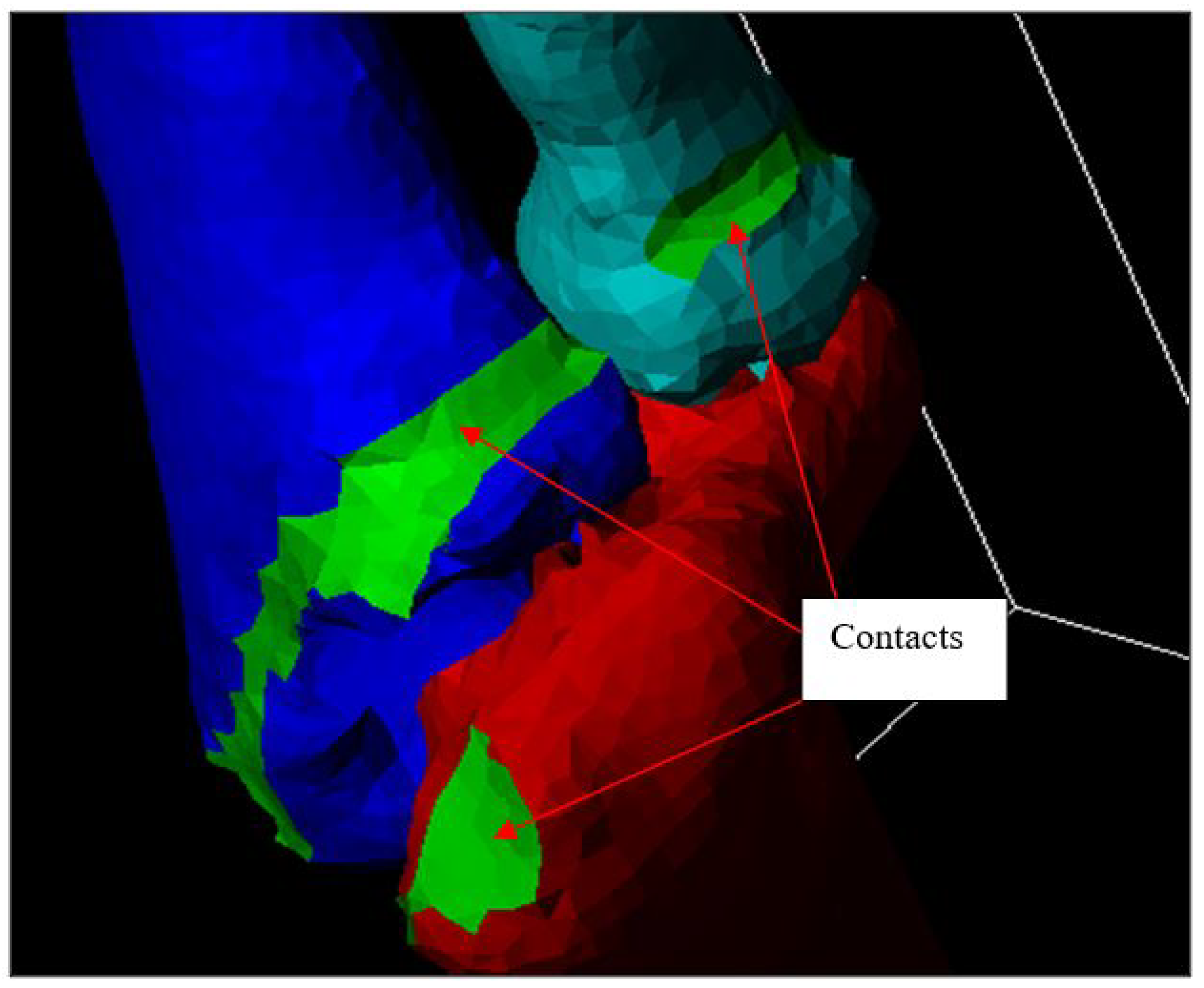
Figure 12.
Bone and cartilage contacts
3.2.5. Material Properties
The linear-elastic material properties for elbow parts need to be defined before exporting the model into ANSYS for FEA. There are three types of material property definitions such Placeholder, Homogeneous, and Grey scale. Homogeneous material type approach was adopted wherein constant values for Mass Density, Young’s Modulus, and Poisson’s Ratio are consolidated into a single linear-elastic material property definition. This simplifies the representation of material properties within the model, allowing for streamlined analysis and computation. Material properties for the ulna, radius, humerus, cartilage and ligaments were obtained from literature [26,35,36,37] (see Table 1) to ensure that the model accurately reflects the mechanical behavior of the anatomical structures within the elbow joint.
In the final step before exporting the 3D model into ANSYS, the element types were defined as all tetrahedral. Additionally, the contact elements were exported as the contact surface. Throughout this process, consistency was maintained in the choice of units, with meters being used consistently when ScanFE exported the node coordinates from the model.
3.2.6. 3D Elbow Model with Different Angles of Flexion and Forearm Configurations
To accurately model the elbow joint across various angles of flexion and forearm positions (pronation or supination), the humerus and the ulna-radius were segmented into separate entities. This segmentation allowed to simulate the complex bio-mechanics of the joint more effectively. The selection of flexion angle ranges was informed by experimental data obtained in literature [1] ensuring that the model reflects realistic physiological ranges of motion. By incorporating these data-driven parameters, the aim is to to achieve a more accurate representation of the dynamic behavior of the elbow joint under different loading conditions. Table 2 outlines the specific ranges of flexion angles considered in the model, providing a comprehensive reference for the simulated scenarios.
Simpleware CAD module offers interactive and intuitive tools for CAD import and integration with 3D images4. The resulting combined models can then be exported as multi-part CAD models and converted automatically into multi-part finite elements. Often the most difficult procedure in medical implant finite element simulations is to combine the image data of the bone with the CAD data of the implant. Previous techniques often leave overlaps and gaps where the bone meets the implant, which can cause contact issues during the simulation. Simpleware CAD module allows triangulated CAD data to be merged with the voxel data of the medical image quickly and robustly.

Table 2.
Model of the elbow joint with different angles of flexion and forearm orientation [1].
Table 2.
Model of the elbow joint with different angles of flexion and forearm orientation [1].
| Forearm orientation | Angle of flexion |
|---|---|
| Pronation | 5° |
| Pronation | 30° |
| Pronation | 45° |
| Pronation | 60° |
| Pronation | 75° |
| Pronation | 90° |
| Supination | 5° |
| Supination | 30° |
| Supination | 45° |
| Supination | 60° |
| Supination | 75° |
| Supination | 90° |
The process is illustrated in Figure 13 and Figure 14. The main step is to convert the CAD/STL data from a surface into the image data. This is done by voxelizing the CAD volume. Voxelization is a process where the surface is converted to voxels using a distance function to encode the CAD data. In the established model, a combination of accurate and robust conversions has been used to achieve the best desired results. The robust conversion artificially pads the CAD surface to generate a volume from an unsigned distance function where as the accuracy conversion requires manifold objects with closed volume.
3.2.7. Ligament Modeling around the Elbow Joint
Modeling ligaments presented a significant challenge, as CT scans did not provide meaningful data on ligament or soft tissue structures. To address this limitation, MRI data, which offers higher resolution and better visualization of ligaments, was used. By utilizing MRI images, precise ligament shapes for modeling were extracted in ScanIP, a process that enabled to achieve more accurate anatomical representations. Once the ligament shapes were extracted, ScanCAD was employed to connect these ligaments to the elbow bone model. This allowed to integrate the ligaments seamlessly with the bone structure, creating a cohesive and anatomically accurate representation of the elbow joint.
In the next section, the details of how the ligaments and cartilage were modeled will be presented, outlining the methods and techniques used to overcome the challenges posed by the lack of CT data and achieve high-fidelity anatomical representations. Through careful integration of MRI data and advanced modeling techniques, a comprehensive model that accurately reflects the complex anatomy of the elbow joint was created.
Magnetic Resonance Imaging (MRI) data of a 28-year-old healthy male human elbow (obtained with a 1.5-T commercial MR system) were used to extract the 3D geometry of the ligaments around the elbow. Data was imported into ScanIP and two masks were created, the Anterior Medial Collateral Ligament (AMCL) and the Lateral Collateral Ligament (LCL). Ligament mechanical properties were defined as in table (Table 3) The second step after modeling the ligaments was to use Simpleware CAD module manipulation feature to attach the ligament to the elbow bone model. The final step was to import the elbow joint model with the ligament into ScanFE to generate a volume mesh ready to be exported into Ansys for finite element analysis (FEA). Figure 15 and Figure 16 show the process in modeling the ligaments.
3.2.8. Cartilage Modeling
Modeling of the elbow joint cartilage plays an essential role in determining contact surface in finite element analysis. In the adopted approach, the cartilage was modeled as the gap between the surfaces of the ulna-humerus and the radius-humerus. To facilitate contact analysis, two masks were utilised in modeling the cartilage, which were named Cartilage1 and Cartilage2. These masks were assigned appropriate material properties to accurately represent the mechanical behavior of cartilage tissue. Figure 17 and Figure 18 provide a visual representation of the process of modeling the cartilage in Simpleware ScanIP and Simpleware FE module, respectively. These figures illustrate the steps involved in delineating the cartilage regions and assigning the appropriate material properties to ensure realistic simulation outcomes. Through modeling of cartilage and integration into our finite element analysis, the aim is to capture the complex interactions between the articulating surfaces of the elbow joint. This approach enables to simulate the distribution of stresses and strains within the joint.
4. Development of the Boundary Conditions, Contacts and FE Validation
4.1. FE Method Using ANSYS
The 3D FE elbow model developed is then imported into ANSYS (Figure 19). Loading and boundary conditions extracted from experimental data of posterior elbow dislocation shown in [1] are used to validate the model. The FE model is then used to investigate how the ligaments and cartilages behave under different flexion and extension angles. The development procedure of the boundary conditions, contacts, and FE validation is explained in the following subsection.
4.1.1. Boundary Conditions and Constraints
Loading and boundary conditions need to be applied on the elbow model to create similar conditions to the conducted experimental studies [1]. In the used experiment setup, the humerus was completely fixed and the ulna-radius allowed to have vertical movement (see Figure 20). Furthermore, the ulna-radius were cemented in a metal cup and subjected to either an axial force or hyper-extension force. In ANSYS, work was done in the x, y, and z coordinate system. Displacements are modeled as Ux, Uy and Uz and loads are modeled as Fx, Fy and Fz. All units in ANSYS are in SI (Standard International) units. In the axial loading group, the force was modeled in the Fx direction. The humerus was constrained in all degrees of freedom (Ux = 0, Uy = 0, Yz = 0) and the ulna-radius was constrained according to Ux = 0.01 m, Uy = 0, Uz = 0 (see Figure 21). In the group subjected to a hyper-extension force, the force was modeled in the Fz direction. Similarly, the humerus was constrained in all degrees of freedom (Ux = 0, Uy = 0, Uz = 0) and the ulna-radius was constrained according to Ux = 0, Uy = 0, Uz = 0.01 m (see Figure 22). In both groups, ligament attachments to the bone were constrained in all degrees of freedom (Ux = 0, Uy = 0, Uz = 0) (see Figure 23). Table 4 summarizes boundary and loading conditions in FE compared to Table 5 and Table 6 obtained from experimental results [1].
4.1.2. Contact Methods at the Elbow Joint
ANSYS supports both rigid-to-flexible and flexible-to-flexible surface contact elements. These contact elements use a “target surface” and a “contact surface” to form a contact pair. In the established model, surface-to-surface contact elements were used. Surface-to-surface elements are well-suited for applications involving interference fit assembly contact or entry contact, forging, and deep-drawing problems. The surface-to-surface contact elements have several advantages over standard contact elements. These elements support lower and higher order elements on the contact and target surfaces. They also provide better contact results needed for typical engineering purposes, such as, normal pressure and friction stress contour plots. They also have no restrictions on the shape of the target surface.
In the elbow model, eight contact pairs are assigned identification (ID) numbers to configure their properties, which significantly influence the solution results. Default values provided by ANSYS, such as the contact algorithm, friction, penetration tolerance, penalty stiffness, and contact detection, are utilized. The only modification made to the contact behavior is setting it to initial contact.
4.1.3. Static Analysis Type
The last step after building the 3D elbow model and applying all boundaries and loading conditions is to define the analysis type and options. In this step, the solution processor is used to define the analysis type and option, the application loads, the load step options, and also to initiate the finite element solution. The analysis type chosen is based on the loading conditions and the response to calculate. In 3D FE model, static analysis was used to calculate joint nodal stresses and joint nodal displacement. For accuracy and convergence purposes, the load was divided into sub-steps that were configured in the solution controls. 100 sub-steps were used with the maximum of 1000 and the minimum of 20.
5. FE Results and Analysis
5.1. Introduction
The 3D developed finite element model was validated using the experimental investigation results obtained and shown in [1]. Nodal displacement as well as nodal stress were noted while the elbow was in pronation or supination with flexion angles varying from (5°, 30°, 45°, 60°, 90°). In the validation process, a high-risk equation was used to model bone fracture and nodal displacement to model ligament tear or rupture.
5.2. Elbows in Pronation with Flexion Angles Varying from (5°, 30°, 45°, 60°, 90°)
5.2.1. Hyper-Extension Load with 5° of Flexion
In this model similar to the experimental results, nodal displacement was noted in ulna-radius, humerus, and ligaments. The experimental results allowed the development of three mechanisms of elbow dislocation with reproducible stages of dislocation. The first mechanism consists of a combined hyper-extension force and a supination at the elbow joint. Three reproducible stages of dislocation were observed in this mechanism:
- Anterior capsule tearing at the mid-portion.
- Anterior medial collateral and anterior capsule complete tear.
- Posterior displacement of the radius-ulna, and the posterior capsule and radial collateral ligament were left intact.
Similar to the produced experimental result, the FE Results showed posterior displacement of ulna-radius shown in Figure 24 and in Figure 25. High nodal displacement was noted in anterior medial collateral ligament versus small displacement at radial collateral ligament as shown in Figure 26 and Figure 27. Results also showed minimum to zero displacement at the distal of the humerus structure as shown in Figure 28, Figure 29, and Figure 30. Table 7 summarizes the maximum and minimum displacement produced in x, y, and z direction for all ulna-radius, humerus and ligaments.
Model solution produced minimal stresses at the coronoid process and the tip of the radial head shown in Figure 31, and Figure 32. These results could conclude the plain elbow dislocation with no fracture could be produced with the elbow joint being under hyper-extension load and at 5° of flexion. Results also showed minimal stresses at the humerus bone structure shown in Figure 28. Table 8 summarizes maximum and minimum stress values occurring at the coronoid process, tip of the radial head, and humerus.
5.2.2. Axial Load with Angles of Flexion 30°, 45°, and 60°
In this group, results similar to the experimental results posterior ulna-radius displacement were noted in all three models with angles of flexion 30°, 45° and 60°. Figure 33, Figure 34 and Figure 35 show ulna radius posterior displacement of the humerus. Results produced a maximum displacement of 0.01m in ulna-radius structure. High displacements also occurred in all three models at the anterior medial collateral ligament and posterior collateral ligament compared to radial collateral ligaments (Figure 36, Figure 37 and Figure 38). These high displacements may have resulted in a rupture or tear of the medial collateral ligament. Results also showed zero to minimum distal displacement of the humerus structure in all three models (Figure 39, Figure 40 and Figure 41). Table 9, Table 10, and Table 11 summarizes maximum and minimum displacement values occurring at the ulna-radius, ligaments and humerus.
The finite element solution produced high nodal stresses at the radial head tip for all three models with the forearm in pronation and the elbow flexed 30°, 45° and 60° respectively (Figure 42, Figure 43 and Figure 44). High nodal stress at the coronoid process only occurred while the forearm pronated and with the elbow in 60° of flexion. These high stresses could lead to bone fracture since the stress values exceed elastic material properties of the ulna-radius bone structure. Table 12 summarizes all of the stress that occurred at the coronoid process, radial head, and humerus in all three models.
Figure 42.
Nodal Stress at Conoriod Process and Radial Head 30° flexion and in pronation
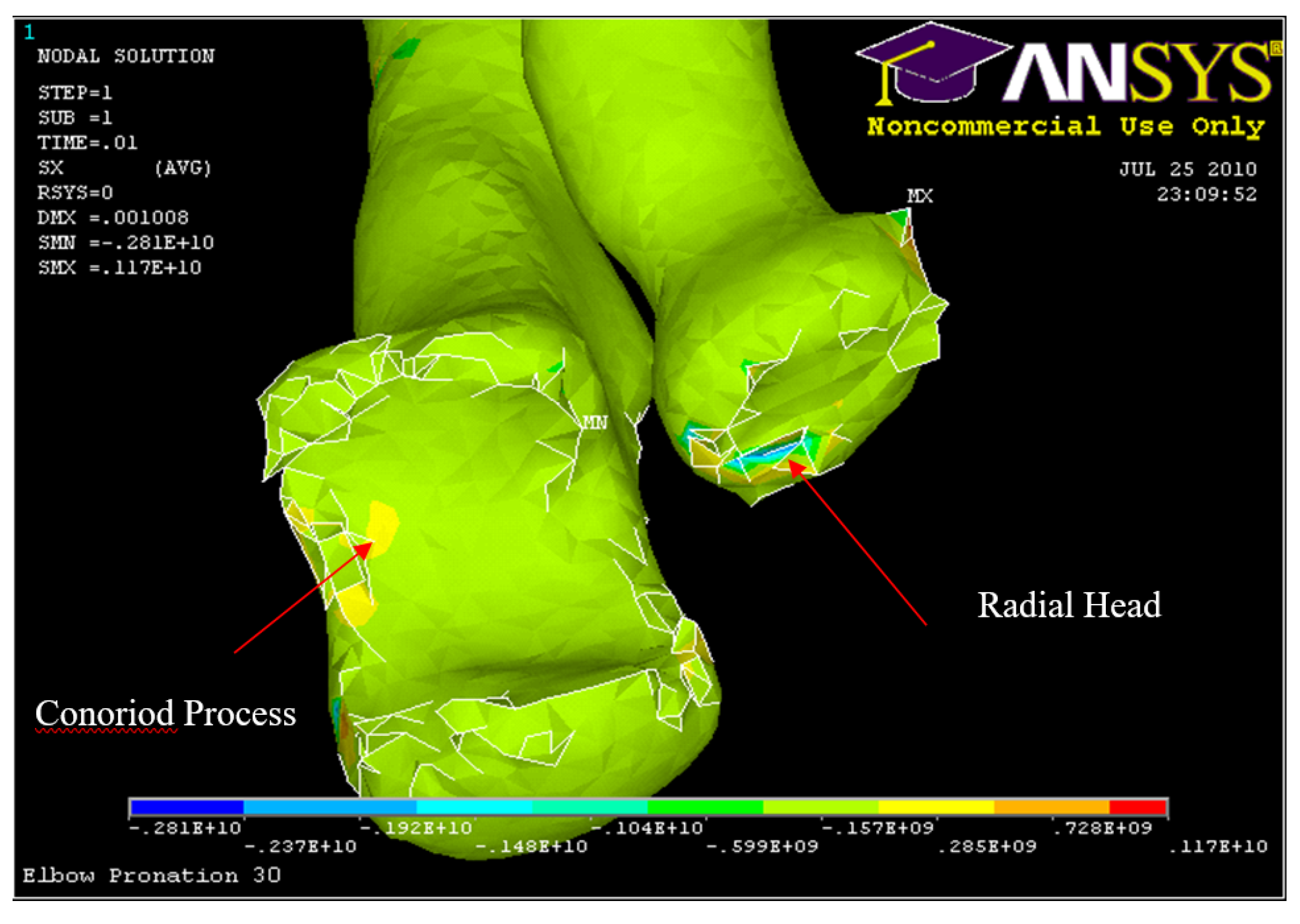
Figure 43.
Nodal Stress at Conoriod Process and Radial Head 45° flexion and in pronation
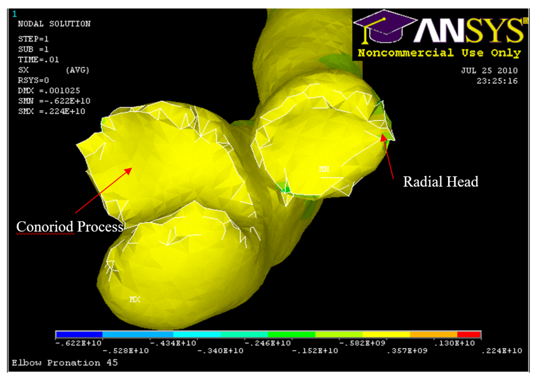
Figure 44.
Nodal Stress at Conoriod Process and Radial Head 60° flexion and in pronation
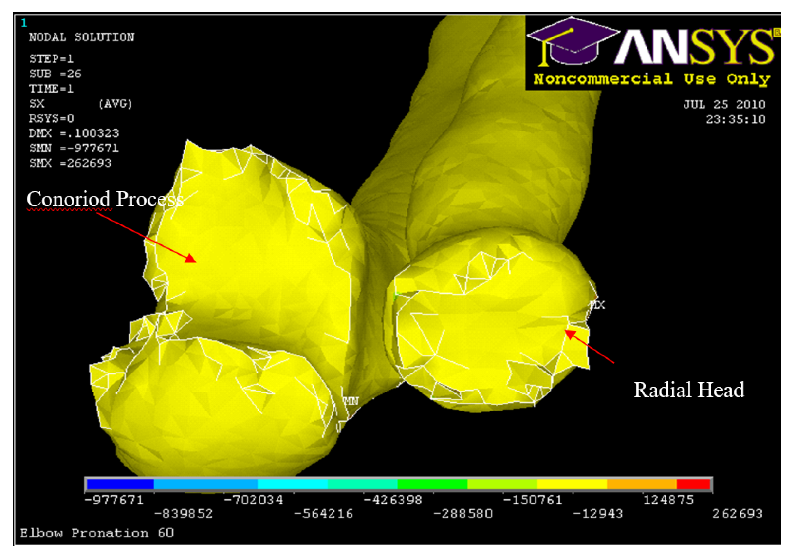
Figure 45.
Nodal Stress at Humerus 30° flexion and in pronation
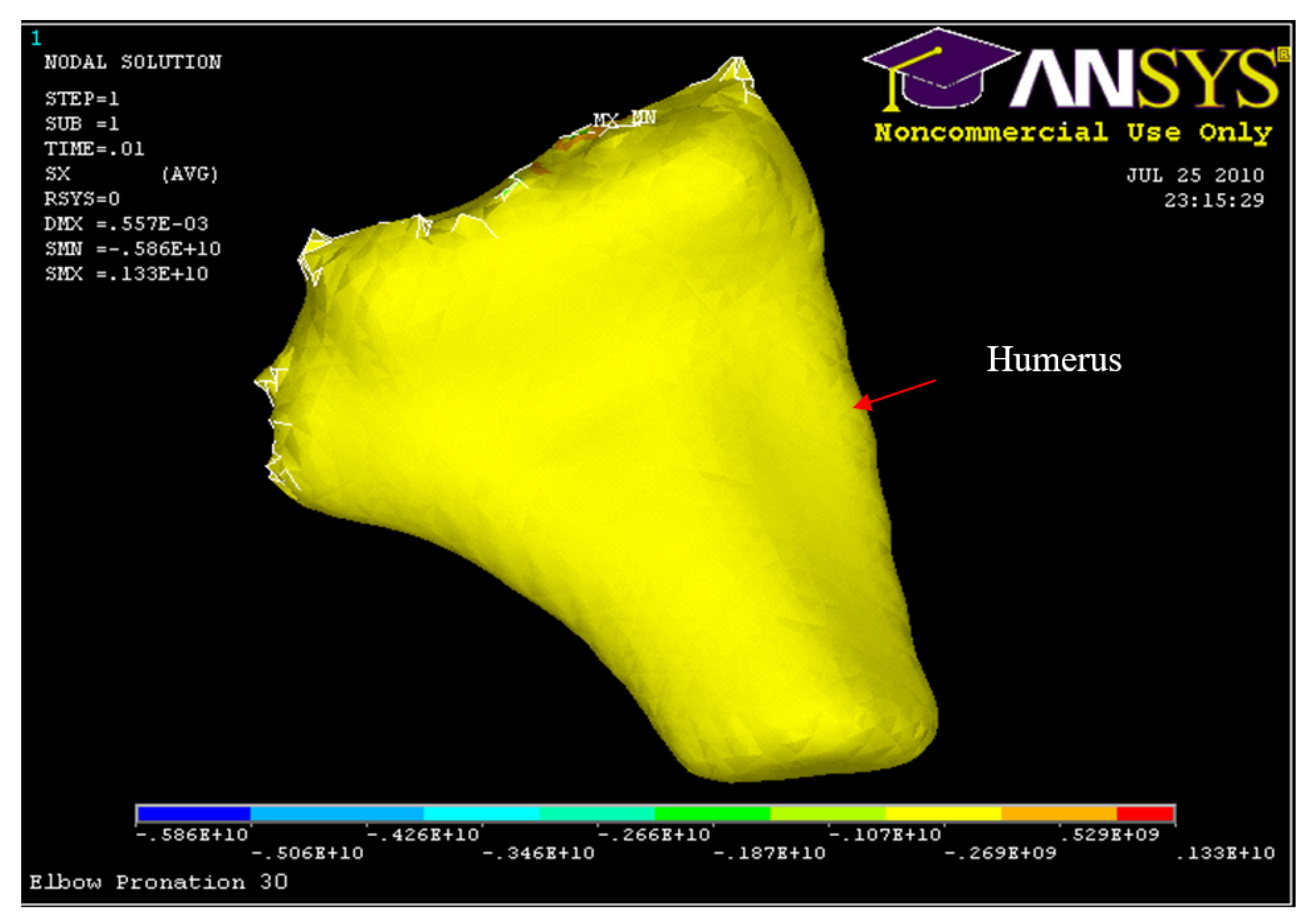
Figure 46.
Nodal Stress at Humerus 45° flexion and in pronation
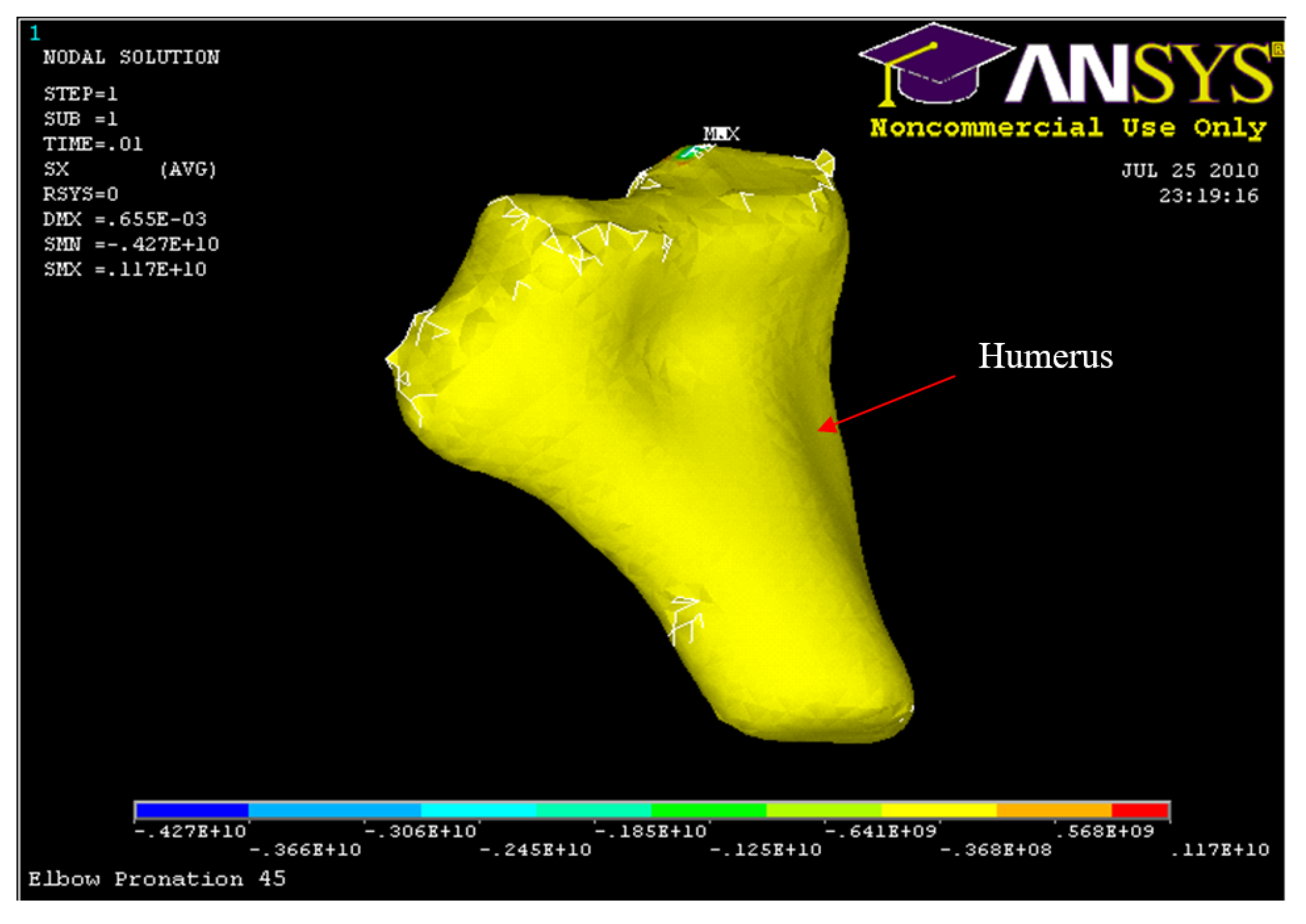
Figure 47.
Nodal Stress at Humerus 60° flexion and in pronation
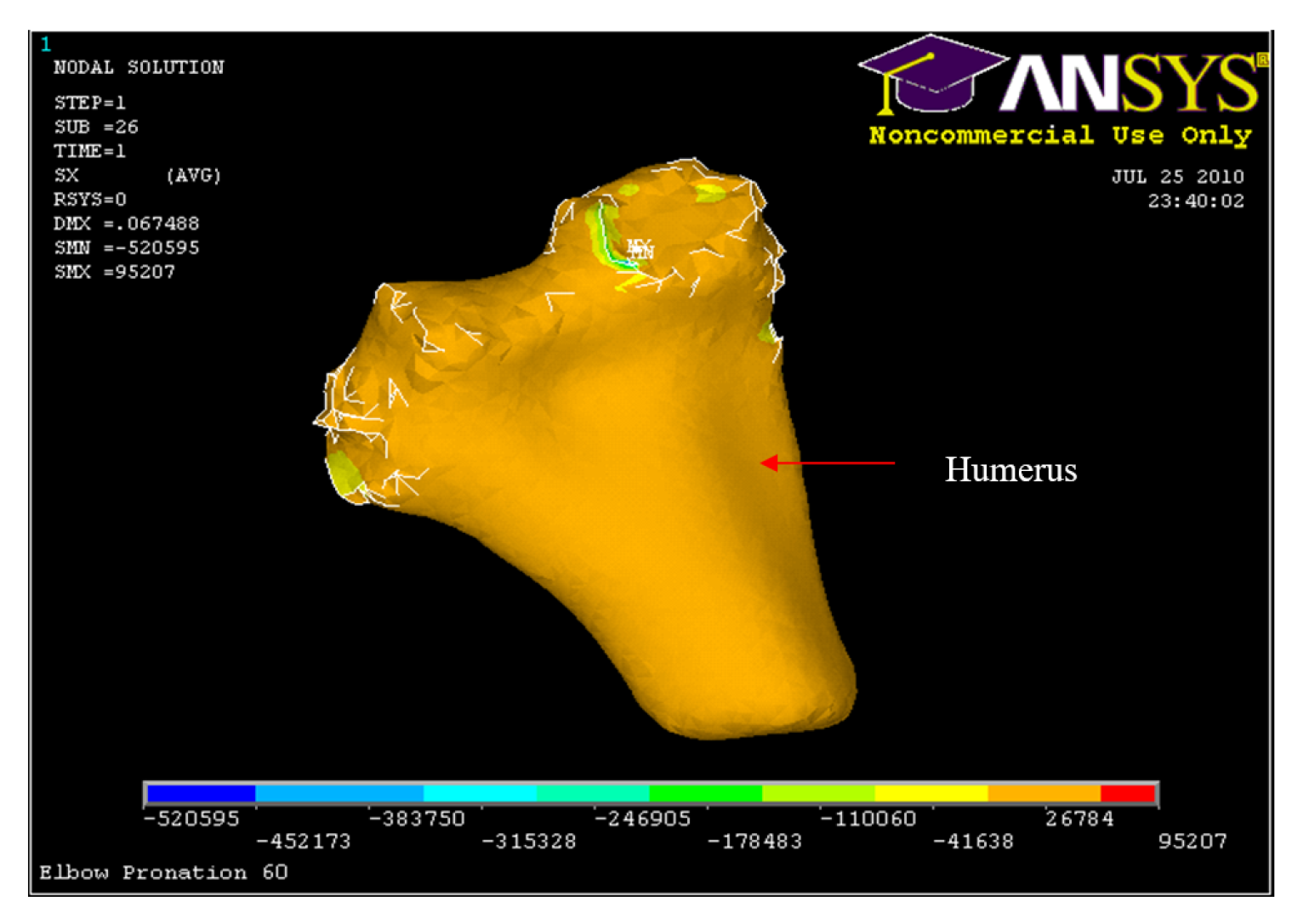
Table 12.
Nodal stresses occurred at coronoid process, radial head and humerus for 30°, 45° and 60° flexion and in pronation
Table 12.
Nodal stresses occurred at coronoid process, radial head and humerus for 30°, 45° and 60° flexion and in pronation
| Structure | Max compressive/tension stress MPa |
|---|---|
| Coronoid process (30° Model) | 59.9 |
| Radial head (30° Model) | 192 |
| Humerus (30° Model) | -107 |
| Coronoid process (45° Model) | 58.2 |
| Radial head (45° Model) | 152 |
| Humerus (45° Model) | 64.1 |
| Coronoid process (60° Model) | 150 |
| Radial head (60° Model) | 150 |
| Humerus (60° Model) | -41.6 |
The three stages of dislocation produced in the experimental results [1] were validated by the FE results as shown below.
- Posterior displacement of the radius and ulna followed by an anterior radial head and/or coronoid process ulna fracture. Additionally, the capsule and collateral ligament were stretched without tears. Figure 48 and Figure 49 illustrates the experimental results where as Figure 33 and Figure 42 illustrates the FE results.
- Ligament complex distal displacement from the radial head and an anterior medial collateral ligament. The medial anterior and lateral posterior capsules were torn. This was followed by a radial collateral and annular ligament complex distal displacement from the radial head and an anterior medial collateral ligament tear as shown in Figure 50.
- Complete medial and lateral tearing of the anterior capsule with the central portion intact. Also, the anterior medial collateral ligament ruptured, followed by a posterior medial collateral ligament tear of the ulna and a posterior capsule rupture as shown in Figure 51.
5.2.3. Axial Load with 90° of Flexion
In this model, significant displacement occurred at the distal humerus (Figure 53) in addition to posterior displacement of the ulna-radius Figure 52. In addition, high displacement was shown at the posterior medial collateral ligament compared to the rest of the ligament complex Figure 54. Table 13 summarizes the maximum and minimum displacements produced in x, y, and z directions for all ulna-radius, humerus and ligaments.
Finite element results showed very high stress (633 MPa) occurring at the distal of the humerus, which will lead to distal humerus fracture (Figure 56) which validates the experimental results of the third mechanism in which it is associated with falling on an outstretched hand, which is rare. The experiments consist of an axial compressive load at the elbow joint with 90° of flexion and either pronation or supination of the forearm. One stage was associated with this mechanism: fracture of the humerus without dislocation of the elbow (See Figure 55).
Conclusion
Based on the detailed developed 3D finite element model and analysis conducted in this study, several key conclusions have been drawn regarding elbow dislocation and instability. The 3D finite element model developed successfully simulates the complex bio-mechanics of the human elbow, providing insights into the stages of dislocation under various loading conditions.These stages were defined based on a common pattern observed in experiments reported by the authors in [1].
-
Stress Concentration and Dislocation Stages
- High stress was observed in the humerus at 90° of flexion and in the radial and coronoid processes at 30°, 45°, and 60° of flexion.
- Three reproducible stages of dislocation were identified, particularly when the elbow was flexed at 30° or 45° with the forearm in either pronation or supination. These stages align with experimental findings and highlight the initial occurrence of bony failures such as fractures of the radial head or ulnar coronoid process, which precede soft tissue tearing.
-
Initial vs. Advanced Stages
- study indicates that in the early stages of most low-impact posterior elbow dislocations, sufficient bony or soft tissue stability is maintained. This suggests that early intervention through closed reduction and early mobilization is feasible and can be effective.
- However, as the dislocation progresses, significant damage to the medial and lateral collateral ligaments is expected. This necessitates more intensive treatment and potentially surgical intervention to restore stability and function.
-
Clinical Implications
- The findings emphasize the importance of timely and appropriate intervention for elbow dislocations. Understanding the stages of dislocation can aid clinicians in deciding the most suitable treatment plan, potentially reducing recovery time and improving outcomes.
- The model’s ability to predict stress distribution and displacement provides a valuable tool for pre-surgical planning and the design of orthopedic devices, enhancing patient-specific treatments.
In summary, the comprehensive analysis using 3D finite element modeling has provided significant insights into the mechanisms of elbow dislocation. These findings support the use of early mobilization for low-impact dislocations and highlight the need for careful management as the injury progresses to prevent severe ligament damage. This research contributes to improved clinical practices and patient outcomes in the treatment of elbow dislocations.
Future Work
The findings from this study lay a solid foundation for further research into the biomechanics of elbow dislocation and instability. However, several areas require additional investigation to enhance our understanding and application of finite element modeling in clinical settings.
- Dynamic Loading Conditions: Extending the model to simulate dynamic loading conditions, such as those experienced during sports or accidental falls, would provide a more comprehensive understanding of dislocation mechanisms.
- Variability in Bone Density and Geometry: Accounting for variations in bone density and geometry among different populations (e.g., age, gender, ethnicity) could refine the model’s applicability and predictive capability.
- Machine Learning Integration: Exploring the integration of machine learning algorithms to predict dislocation outcomes and personalize treatment plans based on large datasets of elbow dislocation cases.
- Real-Time Simulations: Developing real-time simulation capabilities that could be used to guide surgeons during dislocation repair procedures.
References
- Al Kork, S.; Youssef, K.; Said, S.; Beyrouthy, T.; Karar, A.S.; Amirouche, F.; Abraham, E. Exploring the Causes and Effects of Elbow Dislocation: An Ex-Vivo Experimental Investigation Using Papio Anubis Baboon and Human Cadaver Models, 14 April 2024, PREPRINT (Version 1) available at Research Square. [CrossRef]
- Acosta Batlle, J.; Cerezal, L.; Parra, M.; Alba, B.; Resano, S.; Sánchez, J. The elbow: review of anatomy and common collateral ligament complex pathology using MRI. Insights into Imaging 2019, 10. [Google Scholar] [CrossRef] [PubMed]
- Zwerus, E.; Willigenburg, N.; Scholtes, V.; Somford, M.; Eygendaal, D.; van den Bekerom, M. Normative values and affecting factors for the elbow range of motion. Shoulder & Elbow 2017, 11, 175857321772871. [Google Scholar] [CrossRef]
- Magra, M.; Caine, D.; Maffulli, N. A Review of Epidemiology of Paediatric Elbow Injuries in Sports. Sports medicine (Auckland, N.Z.) 2007, 37, 717–735. [Google Scholar] [CrossRef] [PubMed]
- Reichert, I.; Ganeshamoorthy, S.; Aggarwal, S.; Arya, A.; Sinha, J. Dislocations of the elbow – An instructional review. Journal of Clinical Orthopaedics and Trauma 2021, 21, 101484. [Google Scholar] [CrossRef] [PubMed]
- Shanley, E.; Thigpen, C.A.; Boes, N.; Bailey, L.; Arnold, A.; Bullock, G.; Kissenberth, M.J. Arm injury in youth baseball players: a 10-year cohort study. Journal of Shoulder and Elbow Surgery 2023, 32, S106–S111. [Google Scholar] [CrossRef]
- Rezaie, N.; Gupta, S.; Service, B.C.; Osbahr, D.C. Elbow Dislocation. Clinics in Sports Medicine 2020, 39, 637–655. [Google Scholar] [CrossRef]
- Josefsson, P.O.; Nilsson, B.E. Incidence of elbow dislocation. Acta orthopaedica Scandinavica 1986, 57, 537–538. [Google Scholar] [CrossRef]
- Gong, M.; Wang, H.; Jiang, X.; Liu, Y.; Zhou, J. Traumatic divergent dislocation of the elbow in the adults. International Orthopaedics 2023, 47. [Google Scholar] [CrossRef]
- O’Driscoll, S.W.; Jupiter, J.B.; King, G.J.W.; Hotchkiss, R.N.; Morrey, B.F. The Unstable Elbow. The Journal of Bone and Joint Surgery 2000, 82, 724. [Google Scholar]
- Tyrdal, S.; Olsen, B. Combined hyperextension and supination of the elbow joint induces lateral ligament lesions. An experimental study of the pathoanatomy and kinematics in elbow ligament injuries. Knee Surgery, Sports Traumatology, Arthroscopy 1998, 6, 36–43. [Google Scholar] [CrossRef]
- Tyrdal, S.; Sanderhoff Olsen, B. Combined hyperextension and supination of the elbow joint induces lateral ligament lesions. An experimental study of the pathoanatomy and kinematics in elbow ligament injuries. Knee Surgery, Sports Traumatology, Arthroscopy 1998, 6, 36–43. [Google Scholar] [CrossRef] [PubMed]
- Mühlenfeld, N.; Frank, J.; Lustenberger, T.; Marzi, I.; Sander, A. Epidemiology and treatment of acute elbow dislocations: current concept based on primary surgical ligament repair of unstable simple elbow dislocations. European Journal of Trauma and Emergency Surgery 2022, 48. [Google Scholar] [CrossRef] [PubMed]
- Zhou, X.; Draganich, L.; Amirouche, F. A dynamic model for simulating a trip and fall during gait. Medical engineering & physics 2002, 24, 121–127. [Google Scholar] [CrossRef] [PubMed]
- Huiskes, R.; Chao, E.Y.S. A survey of finite element analysis in orthopedic biomechanics: the first decade. Journal of biomechanics 1983, 16, 385–409. [Google Scholar] [CrossRef]
- Heller, M.O. Chapter 32 - Finite element analysis in orthopedic biomechanics. In Human Orthopaedic Biomechanics; Innocenti, B., Galbusera, F., Eds.; Academic Press, 2022; pp. 637–658. [Google Scholar] [CrossRef]
- Kluess, D. Finite Element Analysis in Orthopaedic Biomechanics. 2010. [Google Scholar]
- Kladovasilakis, N.; Tsongas, K.; Tzetzis, D. Finite Element Analysis of Orthopedic Hip Implant with Functionally Graded Bioinspired Lattice Structures. Biomimetics 2020, 5, 44. [Google Scholar] [CrossRef] [PubMed]
- Kohli, A.; Mathad, M.; V Hosamani, S.; Adagimath, M.K.; Kotturshettar, B.B. Finite element analysis of knee joint implant for varying bio material using ANSYS. Materials Today: Proceedings 2022, 59, 941–950. [Google Scholar] [CrossRef]
- Naoum, S.; Vasiliadis, A.; Koutserimpas, C.; Mylonakis, N.; Kotsapas, M.; Katakalos, K. Finite Element Method for the Evaluation of the Human Spine: A Literature Overview. Journal of Functional Biomaterials 2021, 12, 43. [Google Scholar] [CrossRef]
- Zheng, M.; Zou, Z.; Bartolo, P.; Peach, C.; Ren, L. Finite Element Models of the Human Shoulder Complex: A Review of Their Clinical Implications and Modelling Techniques. International journal for numerical methods in biomedical engineering 2016, 33. [Google Scholar] [CrossRef] [PubMed]
- Taha, Z.; Norman, M.S.; Omar, S.F.S.; Suwarganda, E. A Finite Element Analysis of a Human Foot Model to Simulate Neutral Standing on Ground. Procedia Engineering 2016, 147, 240–245. [Google Scholar] [CrossRef]
- Saha, S.; Roy Chowdhury, A. Application of the Finite Element Method in Orthopedic Implant Design. Journal of long-term effects of medical implants 2009, 19, 55–82. [Google Scholar] [CrossRef]
- Alaneme, K.K.; Kareem, S.A.; Ozah, B.N.; Alshahrani, H.A.; Ajibuwa, O.A. Application of finite element analysis for optimizing selection and design of Ti-based biometallic alloys for fractures and tissues rehabilitation: a review. Journal of Materials Research and Technology 2022, 19, 121–139. [Google Scholar] [CrossRef]
- Herrera, A.; Ibarz, E.; Cegoñino, J.; Lobo, A.; Puértolas, S.; Lopez, E.; Mateo, J.; Gracia, L. Applications of finite element simulation in orthopedic and trauma surgery. World journal of orthopedics 2012, 3, 25–41. [Google Scholar] [CrossRef] [PubMed]
- Xu, G.; Yang, Z.; Yang, J.; Liang, Z.; Li, w. Finite Element Analysis of Elbow Joint Stability by Different Flexion Angles of the Annular Ligament. Orthopaedic surgery 2022. [Google Scholar] [CrossRef]
- Maya-Anaya, D.; Urriolagoitia-Sosa, G.; Romero-Ángeles, B.; Martinez-Mondragon, M.; German-Carcaño, J.M.; Correa-Corona, M.I.; Trejo-Enríquez, A.; Sánchez-Cervantes, A.; Urriolagoitia-Luna, A.; Urriolagoitia-Calderón, G.M. Numerical Analysis Applying the Finite Element Method by Developing a Complex Three-Dimensional Biomodel of the Biological Tissues of the Elbow Joint Using Computerized Axial Tomography. Applied Sciences 2023, 13, 8903. [Google Scholar] [CrossRef]
- Lechosa Urquijo, E.; Blaya Haro, F.; D’Amato, R.; Juanes, Mé; ndez, J.A. Finite Element model of an elbow under load, muscle effort analysis when modeled using 1D rod element. Eighth International Conference on Technological Ecosystems for Enhancing Multiculturality; Association for Computing Machinery: New York, NY, USA, 2021. TEEM’20. pp. 475–482. [Google Scholar] [CrossRef]
- Gupta, A.; Singh, O. Computer Aided Modeling and Finite Element Analysis of Human Elbow. 2016; Vol. 5, pp. 31–38. [Google Scholar] [CrossRef]
- Kahmann, S.L.; Sas, A.; Große Hokamp, N.; van Lenthe, G.H.; Müller, L.P.; Wegmann, K. A combined experimental and finite element analysis of the human elbow under loads of daily living. Journal of Biomechanics 2023, 158, 111766. [Google Scholar] [CrossRef] [PubMed]
- Ye, H.; Yang, Y.; Xing, T.; Tan, G.; Jin, S.; Zhao, Z.; Zhang, W.; Li, Y.; Zhang, L.; Wang, J.; Zheng, R.; Lu, Y.; Wu, L. Anatomical and Biomechanical Stability of Single/Double Screw-Cancellous Bone Fixations of Regan–Morry Type III Ulnar Coronoid Fractures in Adults: CT Measurement and Finite Element Analysis. Orthopaedic Surgery 2023, 15. [Google Scholar] [CrossRef]
- Wake, H.; Hashizume, H.; Nishida, K.; Inoue, H.; Nagayama, N. Biomechanical analysis of the mechanism of elbow fracturedislocations by compression force. Journal of Orthopaedic Science 2004, 9, 44–50. [Google Scholar] [CrossRef] [PubMed]
- Nalbone, L.; Monac, F.; Nalbone, L.; Ingrassia, T.; Ricotta, V.; Nigrelli, V.; Ferruzza, M.; Tarallo, L.; Porcellini, G.; Camarda, L. Study of a constrained finite element elbow prosthesis: the influence of the implant placement. Journal of Orthopaedics and Traumatology 2023, 24. [Google Scholar] [CrossRef] [PubMed]
- Ricotta, V.; Bragonzoni, L.; Marannano, G.; Nalbone, L.; Valenti, A. Biomechanical Analysis of a New Elbow Prosthesis. Design Tools and Methods in Industrial Engineering; Rizzi, C., Andrisano, A.O., Leali, F., Gherardini, F., Pini, F., Vergnano, A., Eds.; Springer International Publishing: Cham, 2020; pp. 812–823. [Google Scholar] [CrossRef]
- Stylianou, A. Computational approaches to study elbow biomechanics. Annals of Joint 2020, 6. [Google Scholar] [CrossRef]
- Sadeghi, S.; Lin, C.Y.; Bader, D.A.; Cortes, D.H. Evaluating Changes in Shear Modulus of Elbow Ulnar Collateral Ligament in Overhead Throwing Athletes Over the Course of a Competitive Season. Journal of Engineering and Science in Medical Diagnostics and Therapy 2018, 1, 041008. [Google Scholar] [CrossRef]
- Kamei, K.; Sasaki, E.; Fujisaki, K.; Harada, Y.; Yamamoto, Y.; Ishibashi, Y. Ulnar collateral ligament dysfunction increases stress on the humeral capitellum: a finite element analysis. JSES International 2021, 5, 307–313. [Google Scholar] [CrossRef] [PubMed]
| 1 | |
| 2 | |
| 3 | Available: https://www.ansys.com/
|
| 4 |
Figure 1.
Elbow anatomy
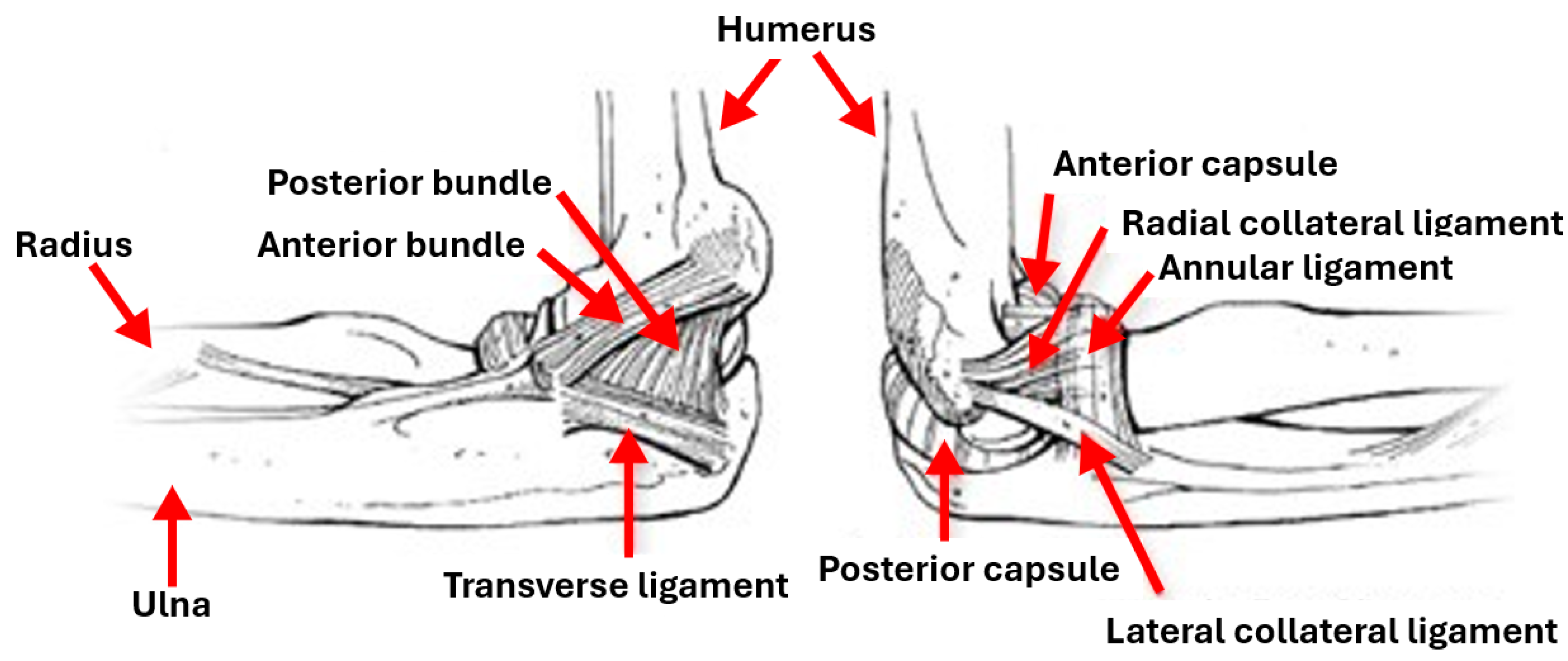
Figure 2.
3D Modeling Procedure followed
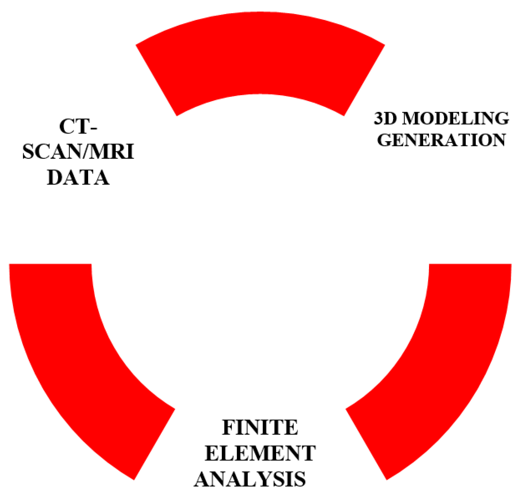
Figure 3.
CT scan data of the elbow joint.
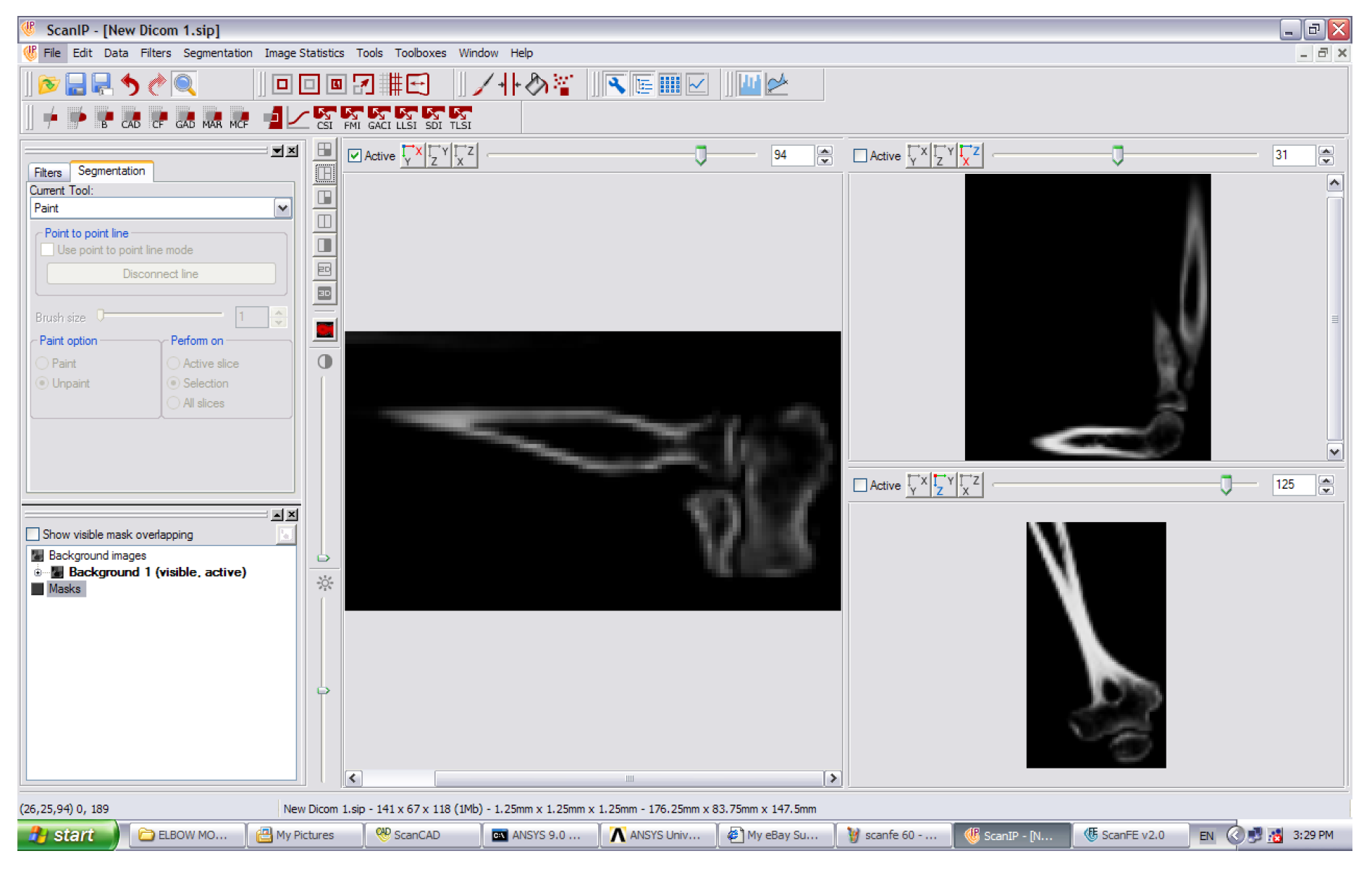
Figure 4.
Medical data processing steps
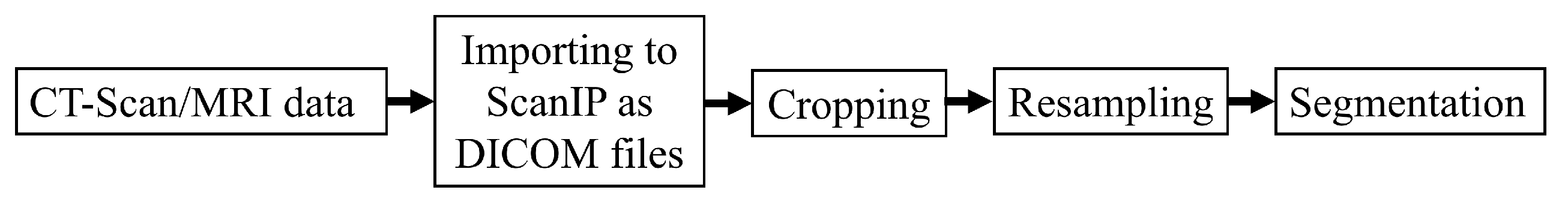
Figure 5.
2D schematic showing mask development of the humerus, ulna and radius.
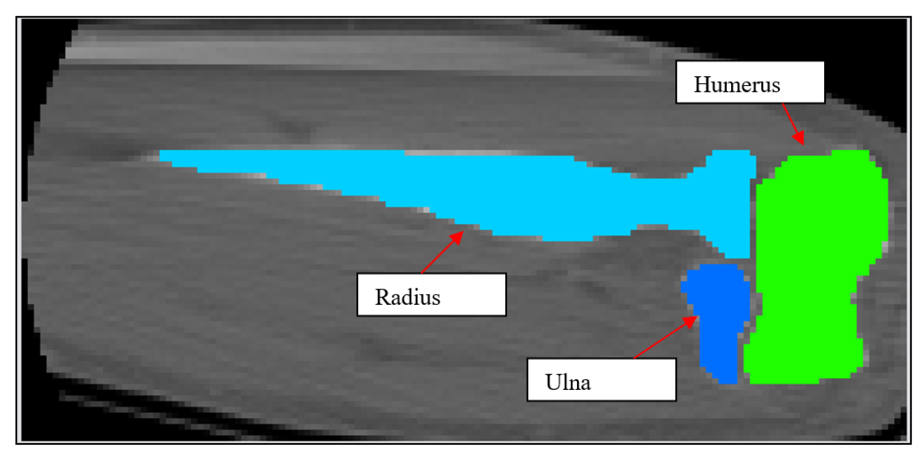
Figure 6.
2D schematic showing mask development of Cartilage 1 and Cartilage 2.
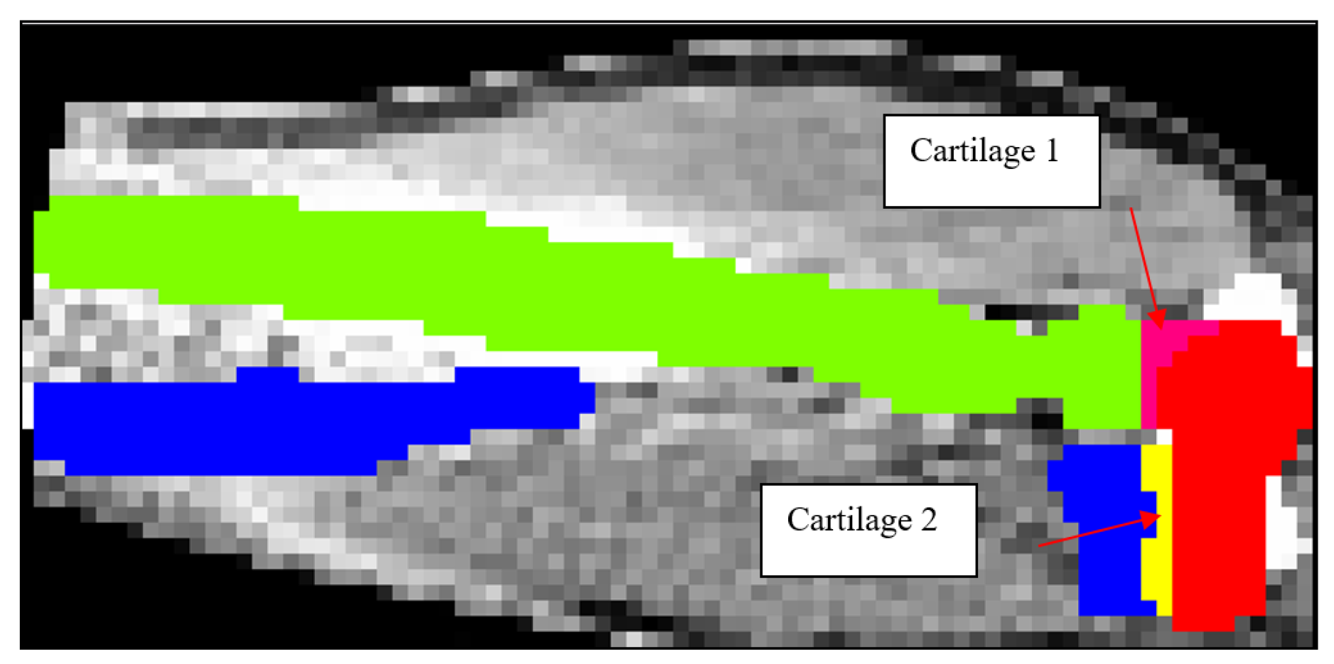
Figure 7.
2D schematic showing mask development of the ligaments.
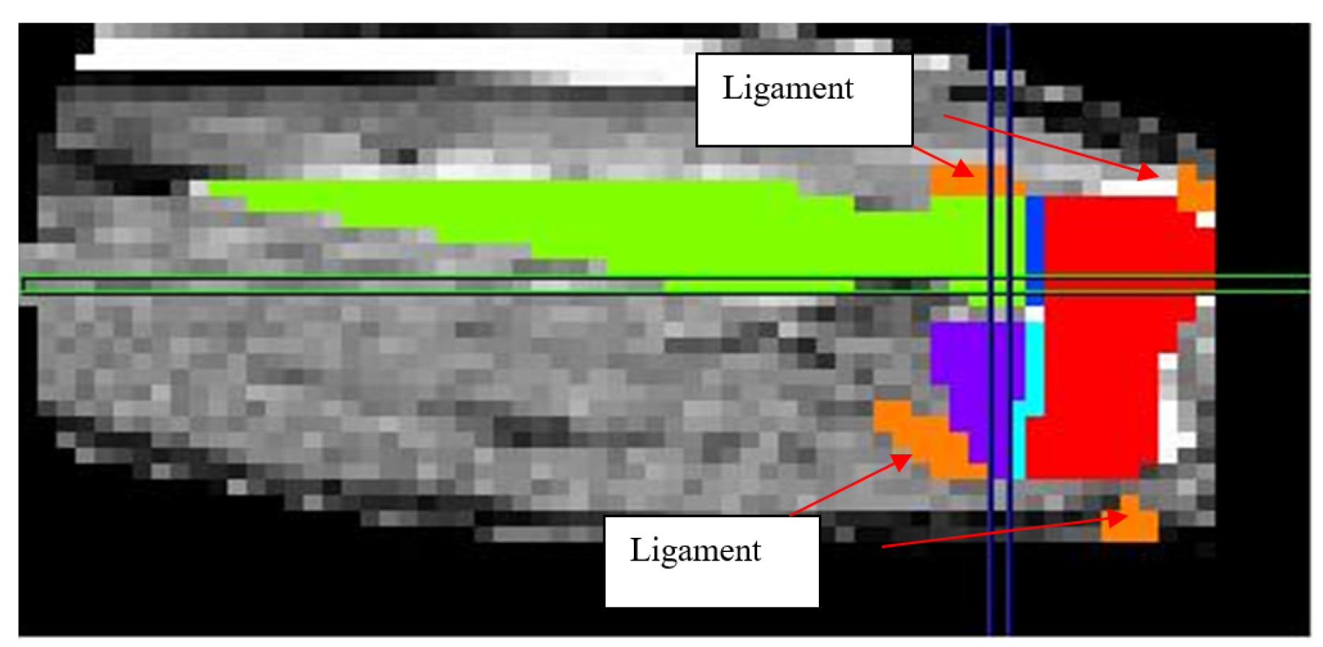
Figure 8.
3D solid model of the elbow joint.
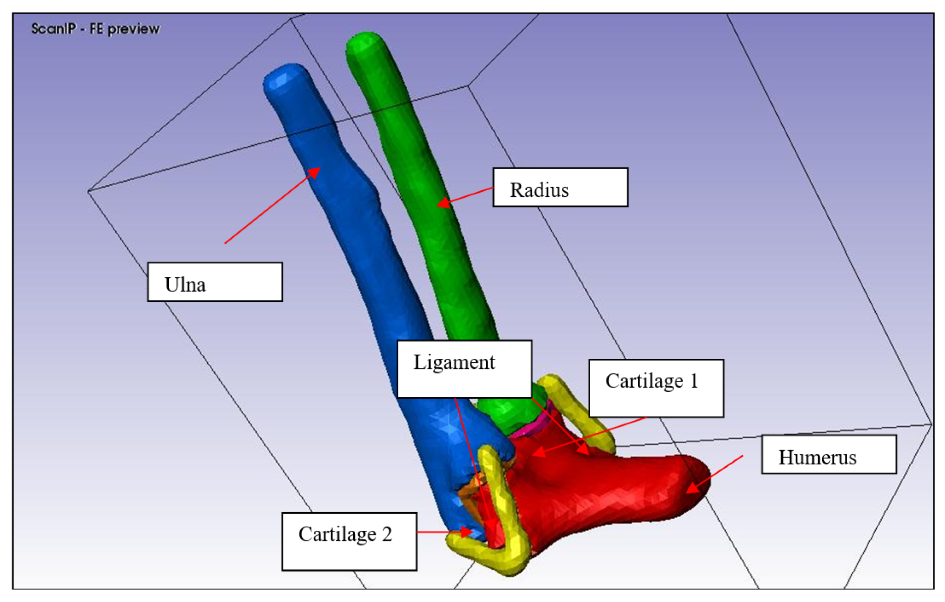
Figure 9.
FE generation without mesh refinement
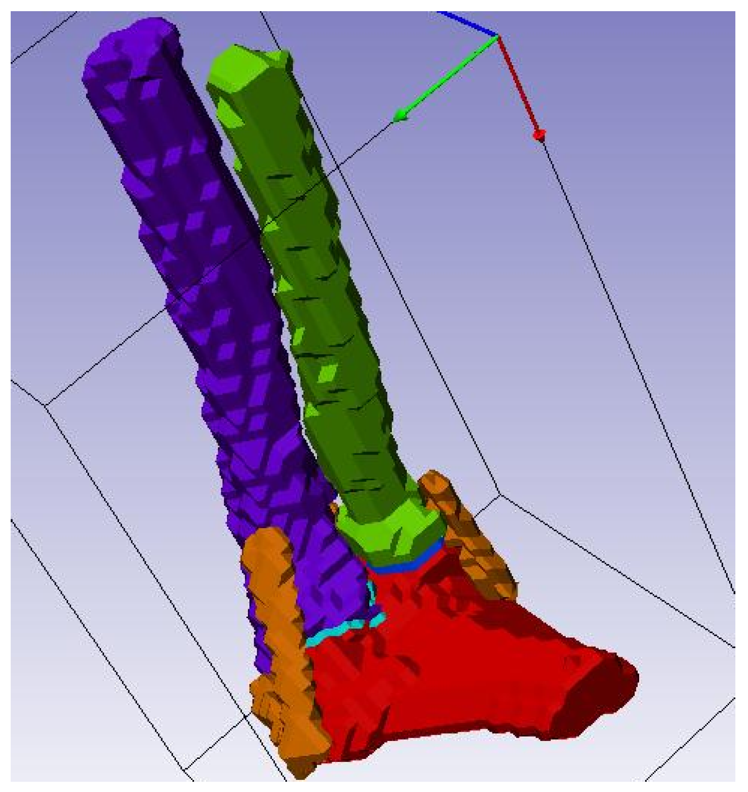
Figure 10.
FE generation with mesh refinement
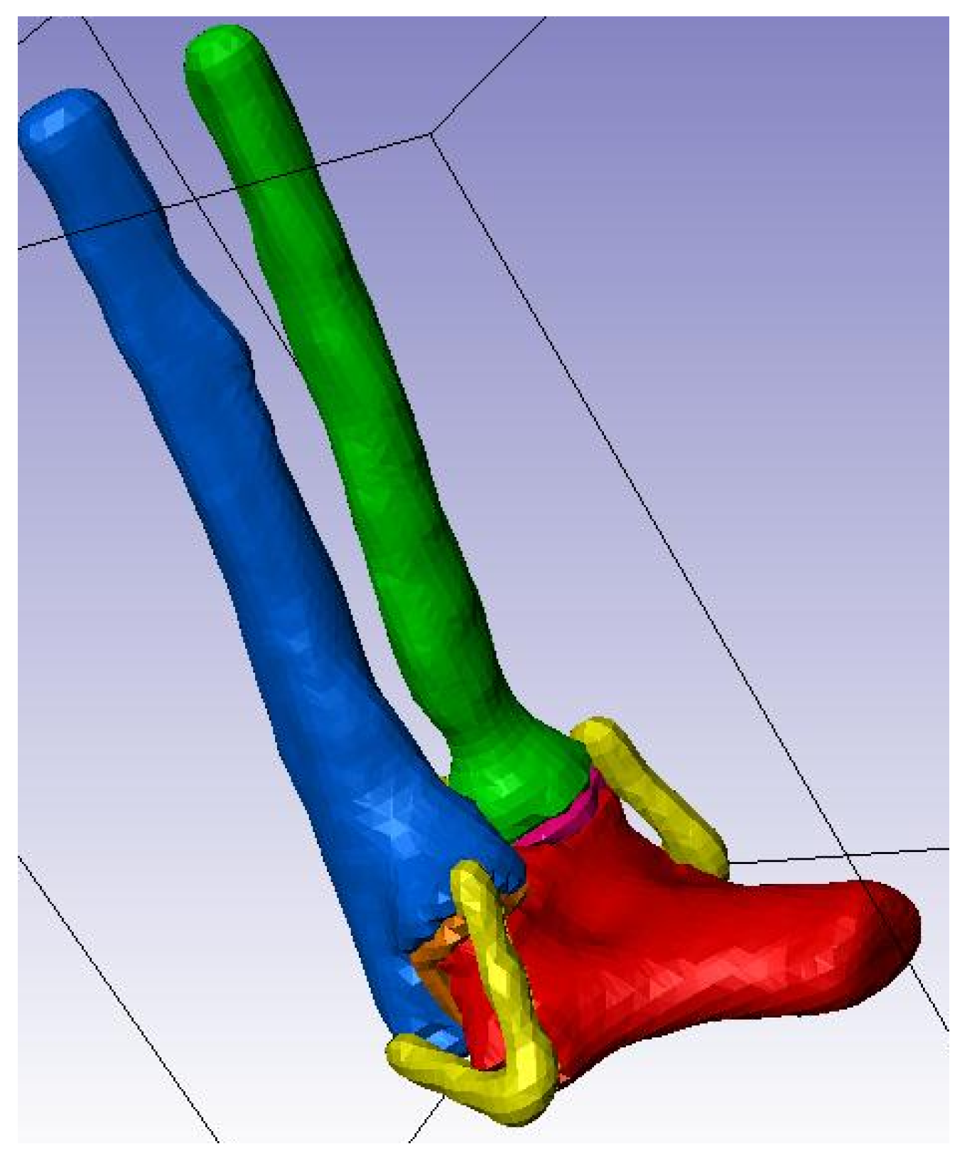
Figure 13.
Humerus and Ulna-Radius manipulation
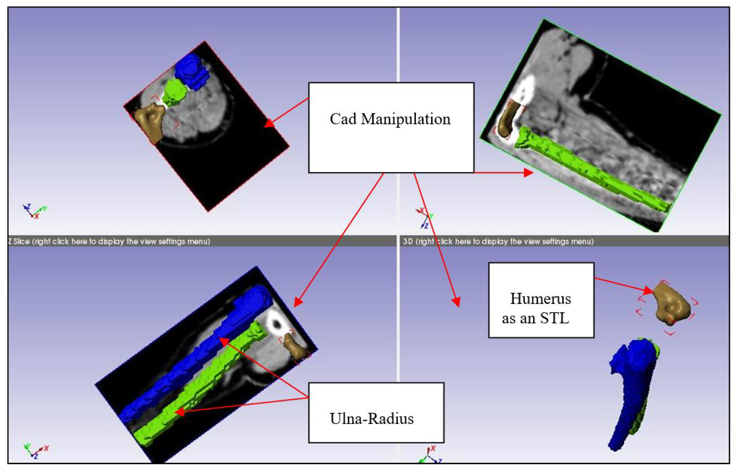
Figure 14.
Elbow joint at 90° of flexion
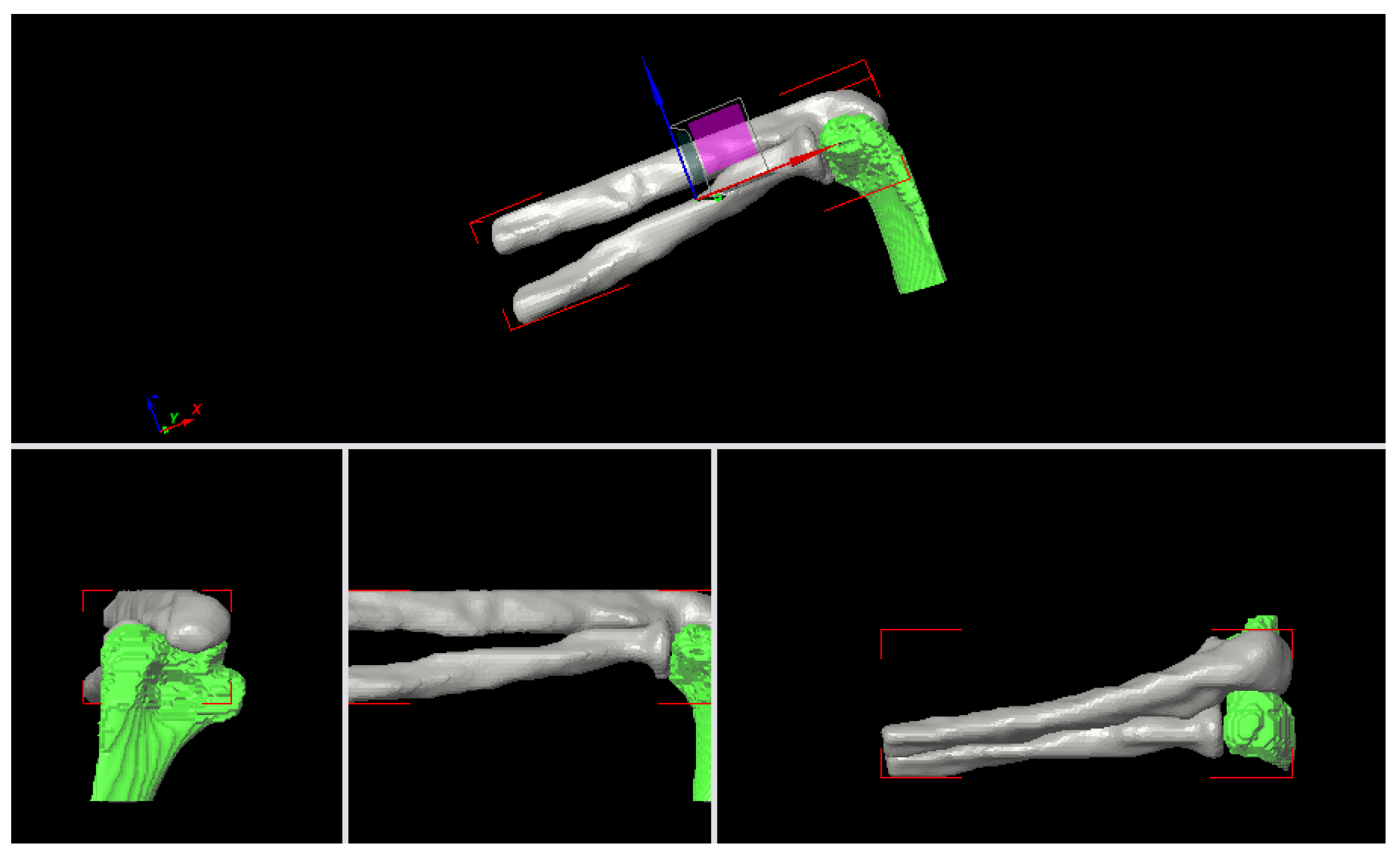
Figure 15.
Radial Collateral Ligament (RCL)
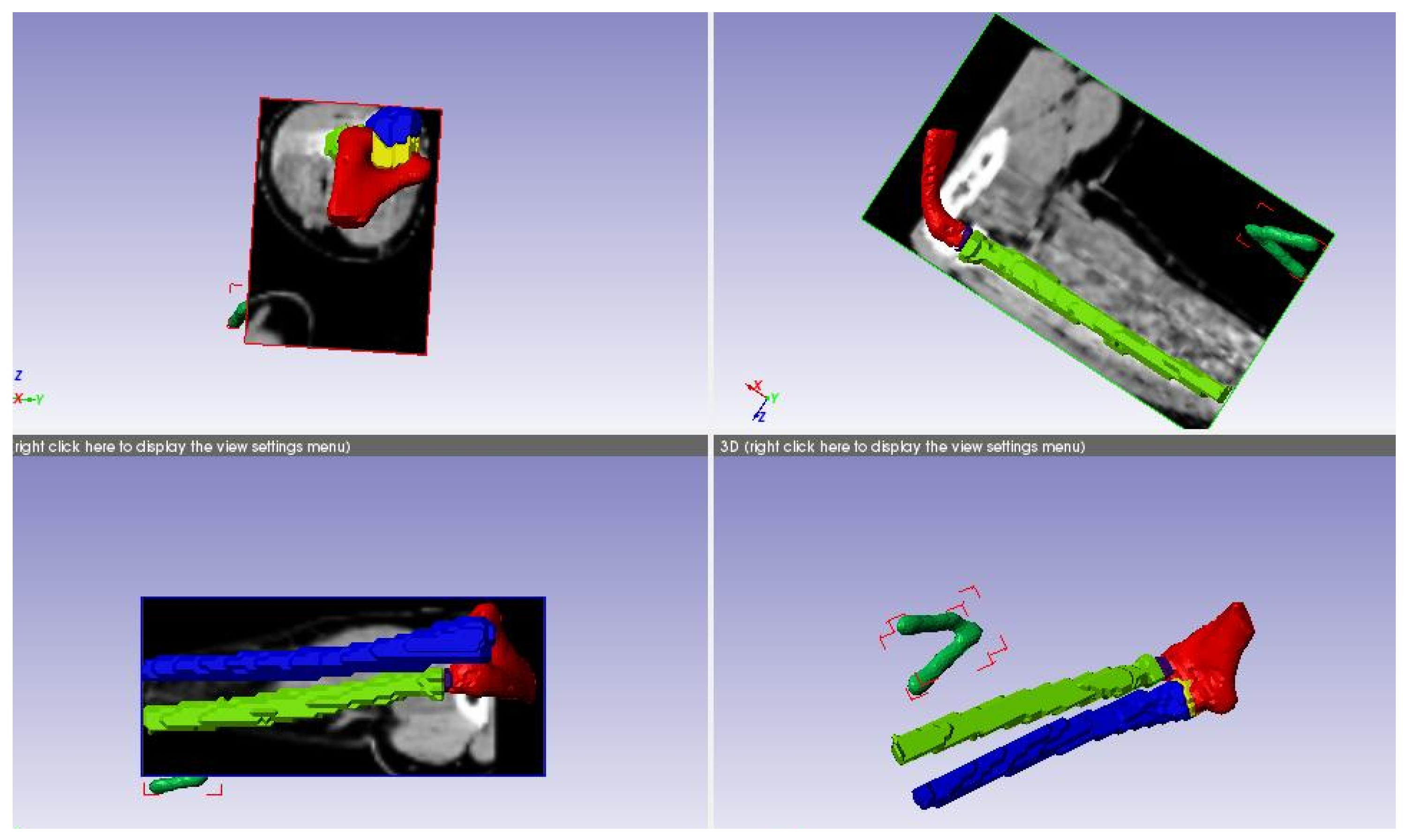
Figure 16.
Ulnar Collateral Ligament.
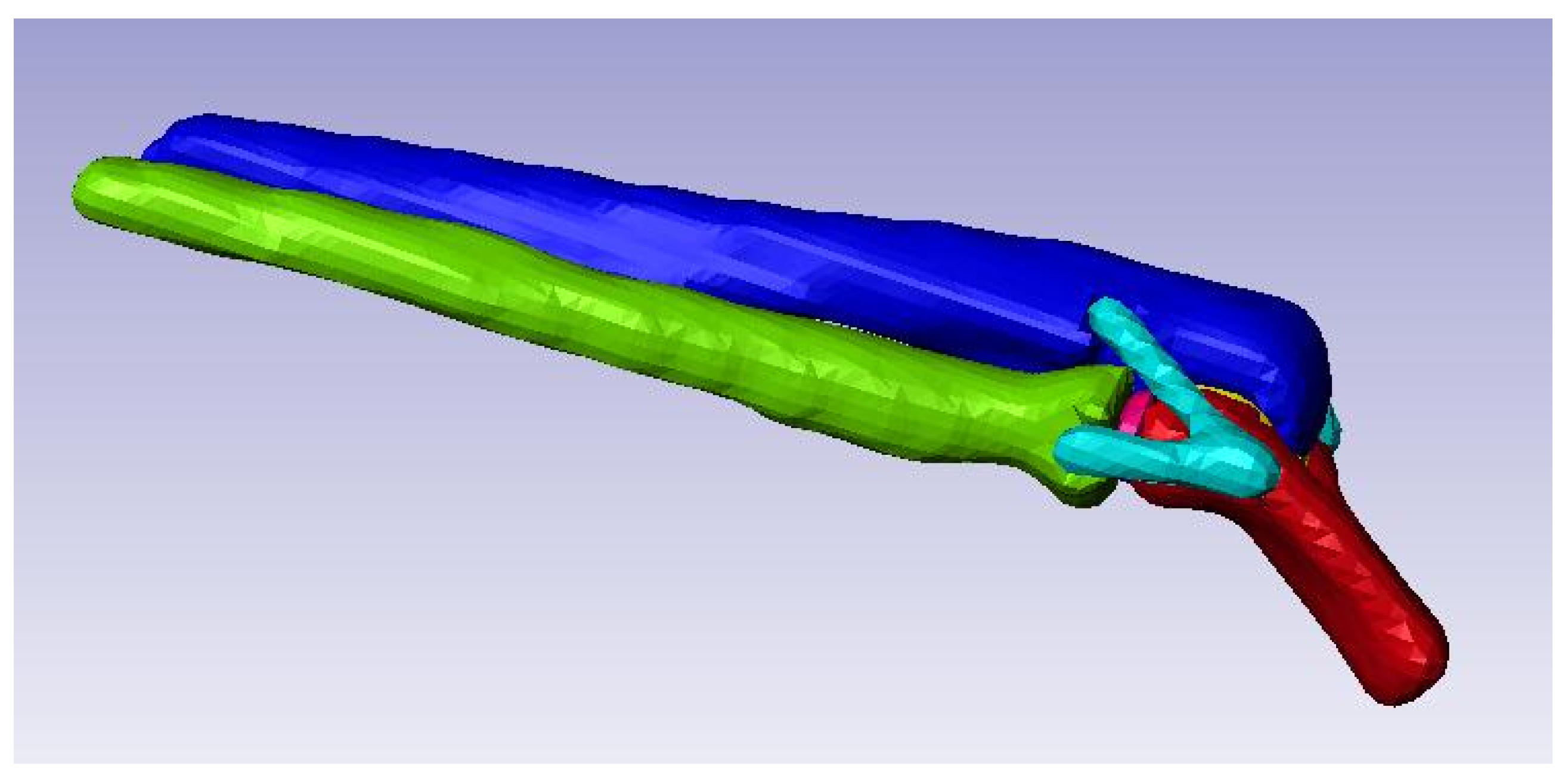
Figure 17.
Cartilage Modeling.
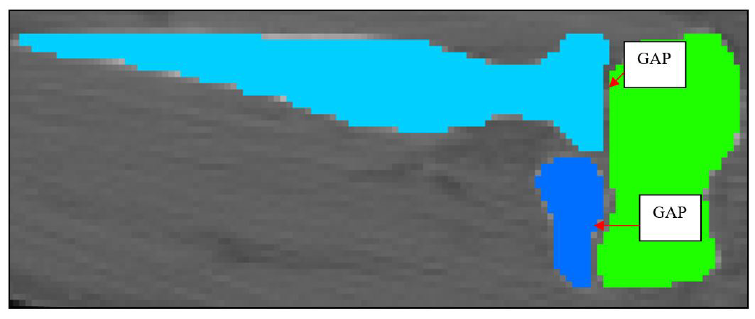
Figure 18.
2D Schematic of Cartilage 1 and Cartilage 2.
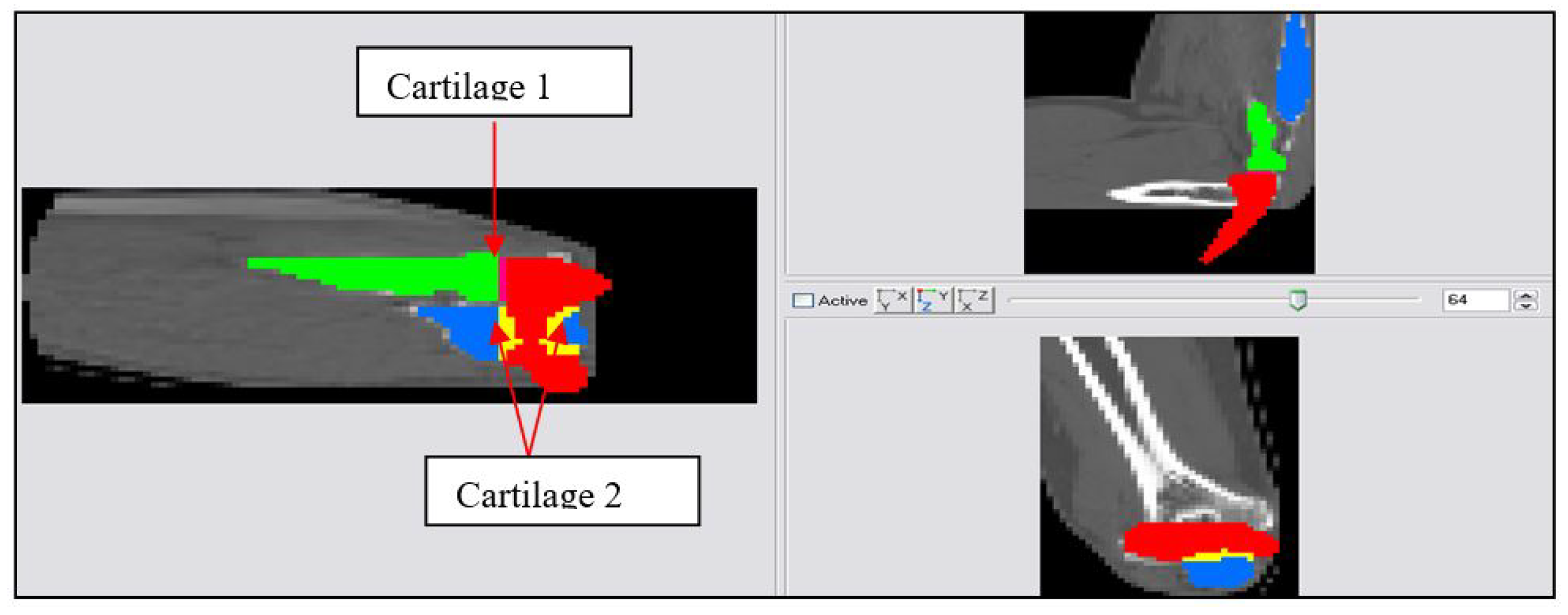
Figure 19.
3D FE model developed in Simpleware.
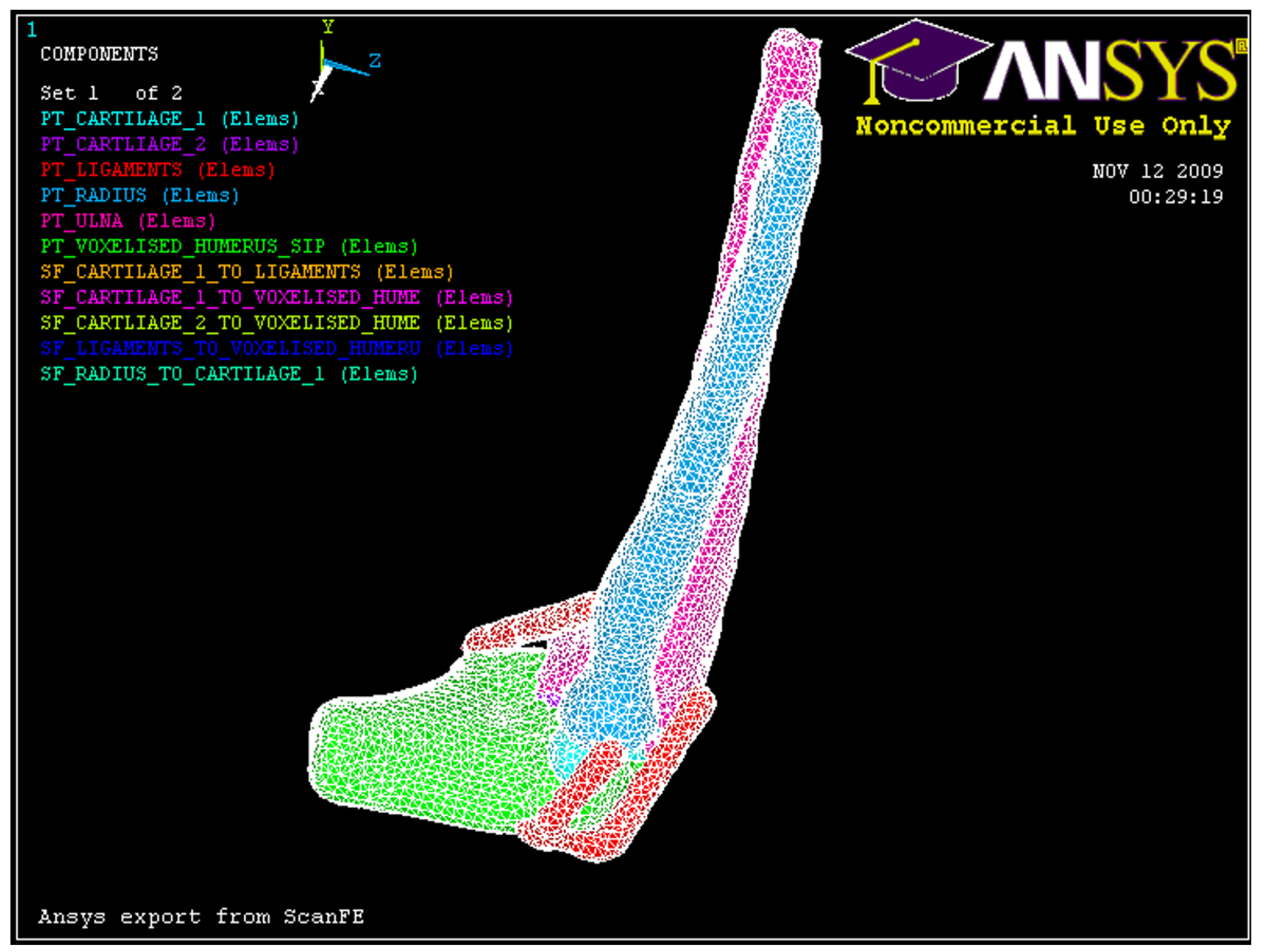
Figure 20.
Loading apparatus used with human cadaver arms [1]
Figure 20.
Loading apparatus used with human cadaver arms [1]
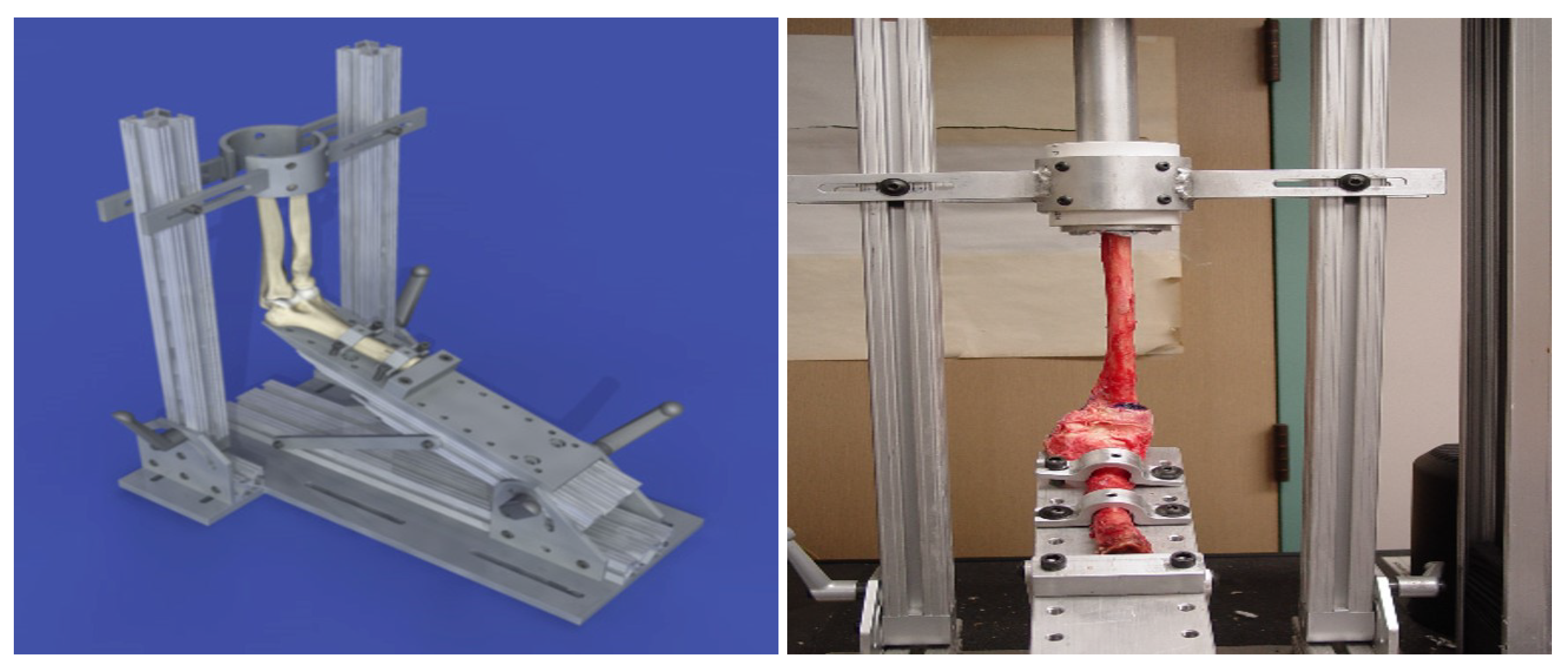
Figure 21.
Axial loading, Fx = 2000 N, Humerus (0.01 m, 0, 0), Ulna-Radius (0, 0, 0).
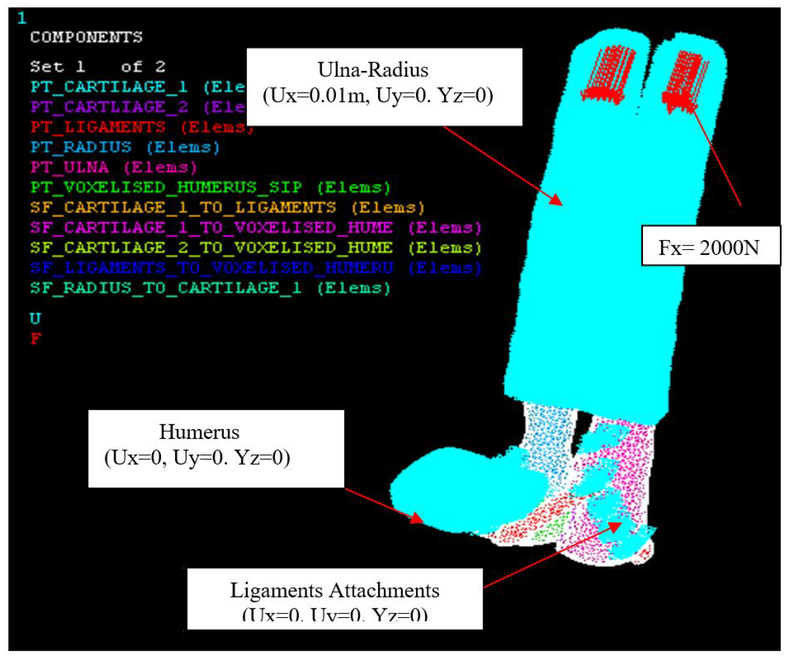
Figure 22.
Hyper-extension loading, Fz = 500 N, Humerus (0, 0, 0), Ulna-Radius (0, 0, 0.01 m).
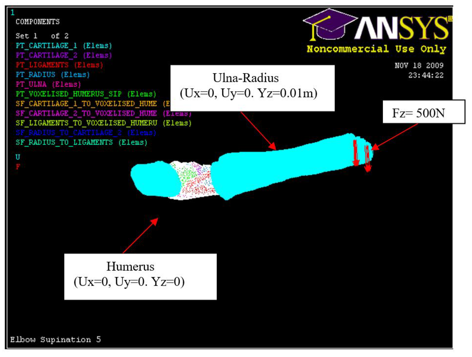
Figure 23.
Ligament attachments (0, 0, 0).
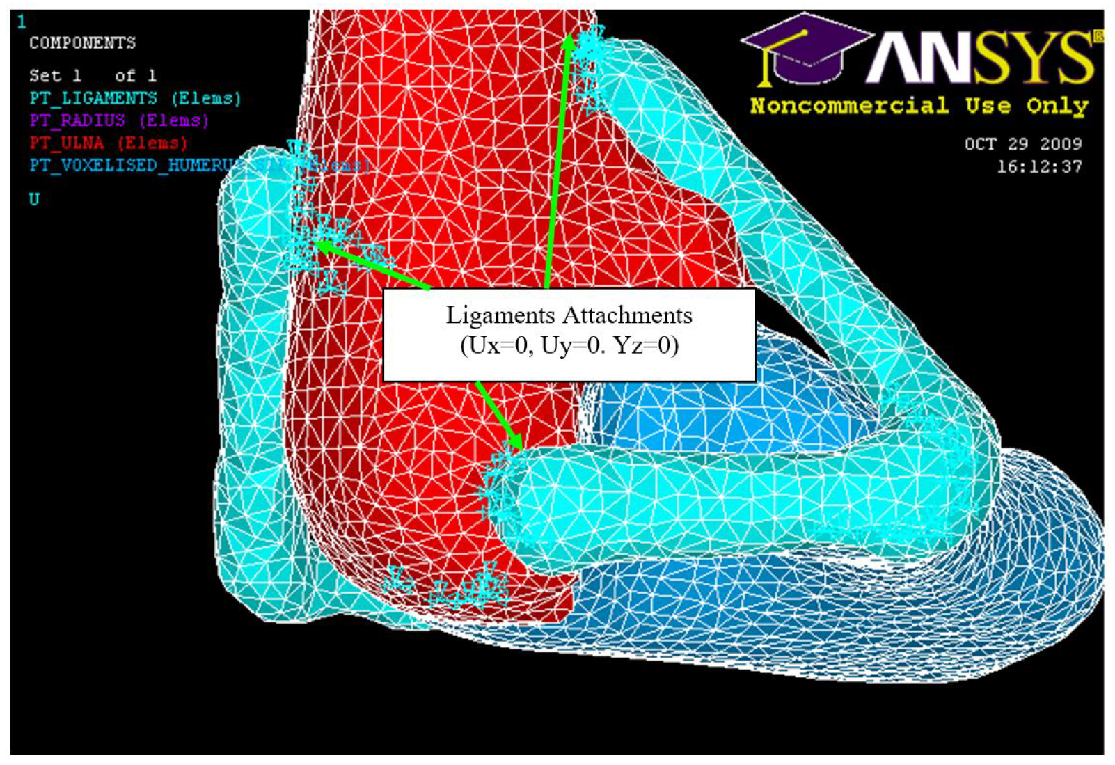
Figure 24.
FE: Posterior Displacement of ulna-radius with 5° of flexion and in pronation
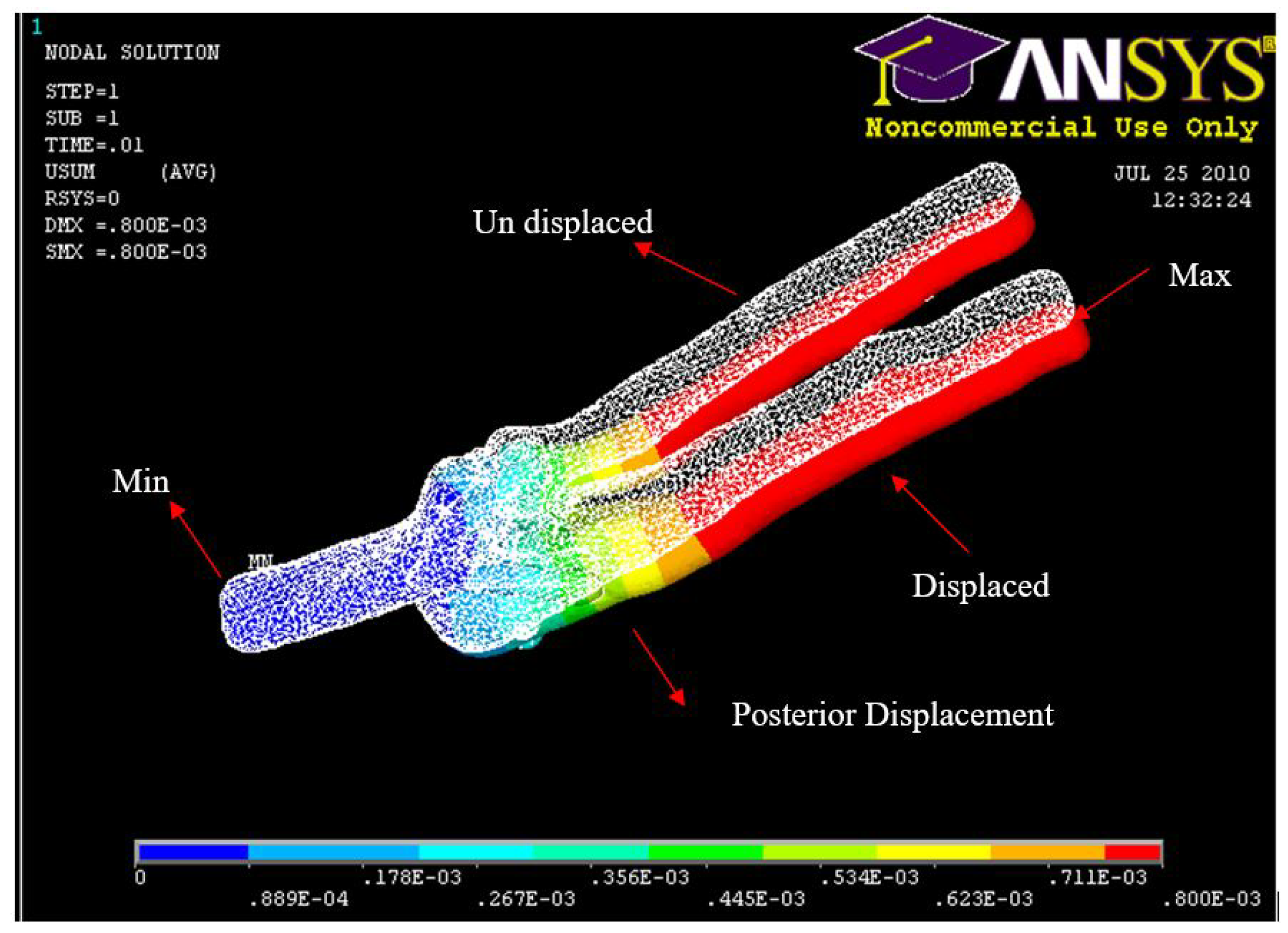
Figure 25.
Experiment: Posterior Displacement of ulna-radius with 5° of flexion and in pronation
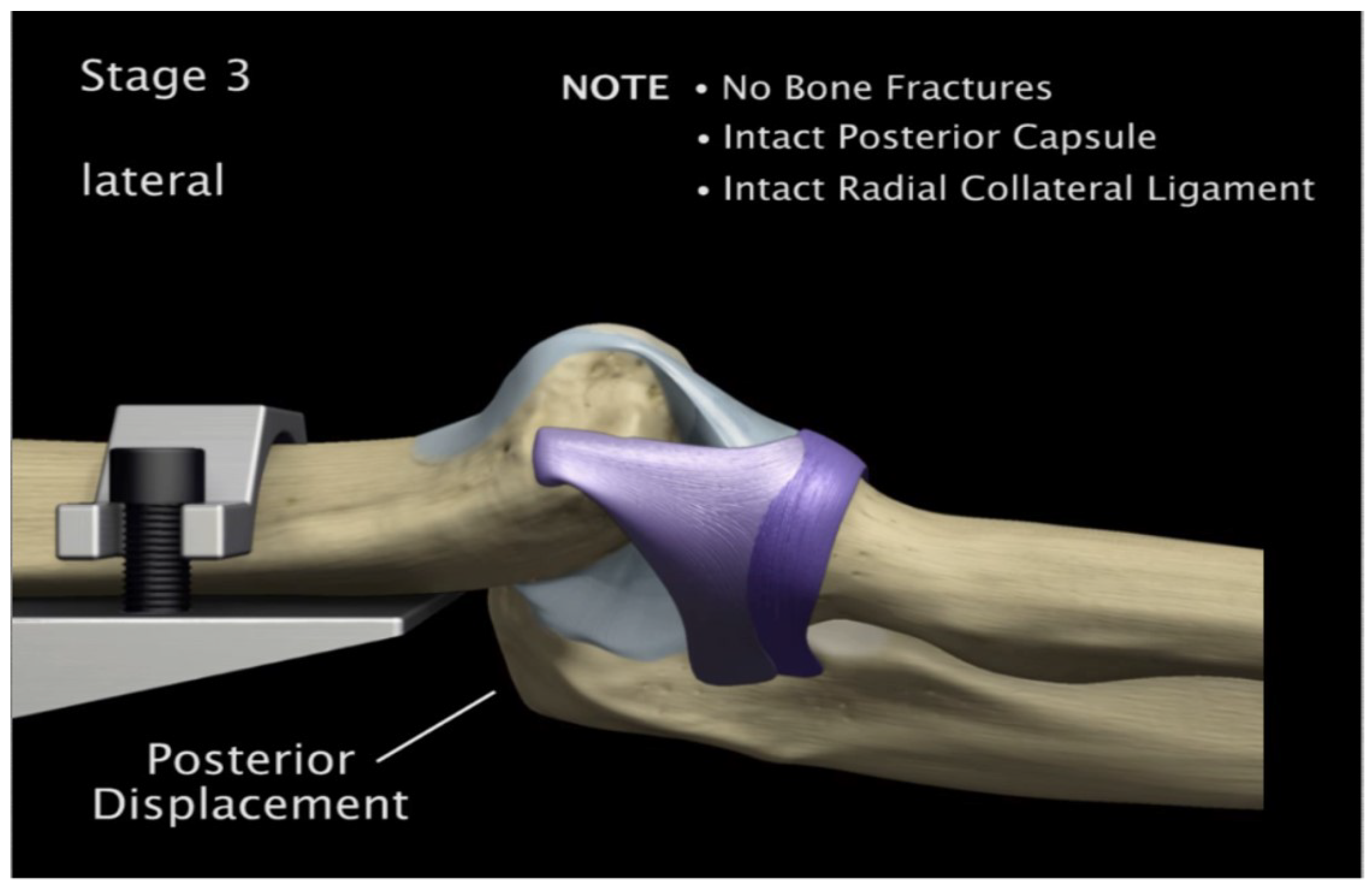
Figure 26.
FE: Displacement of AMCL, PMCL and RCL
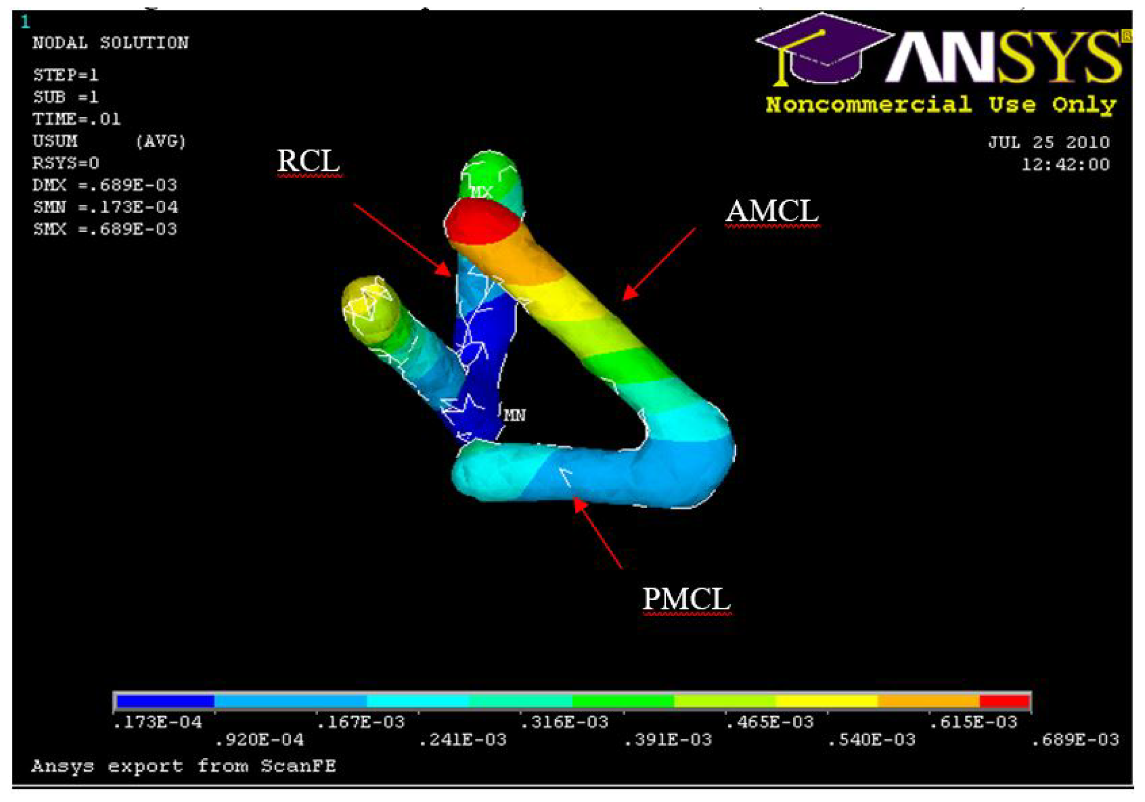
Figure 27.
Experiment: Anterior medial collateral and anterior capsule complete tear
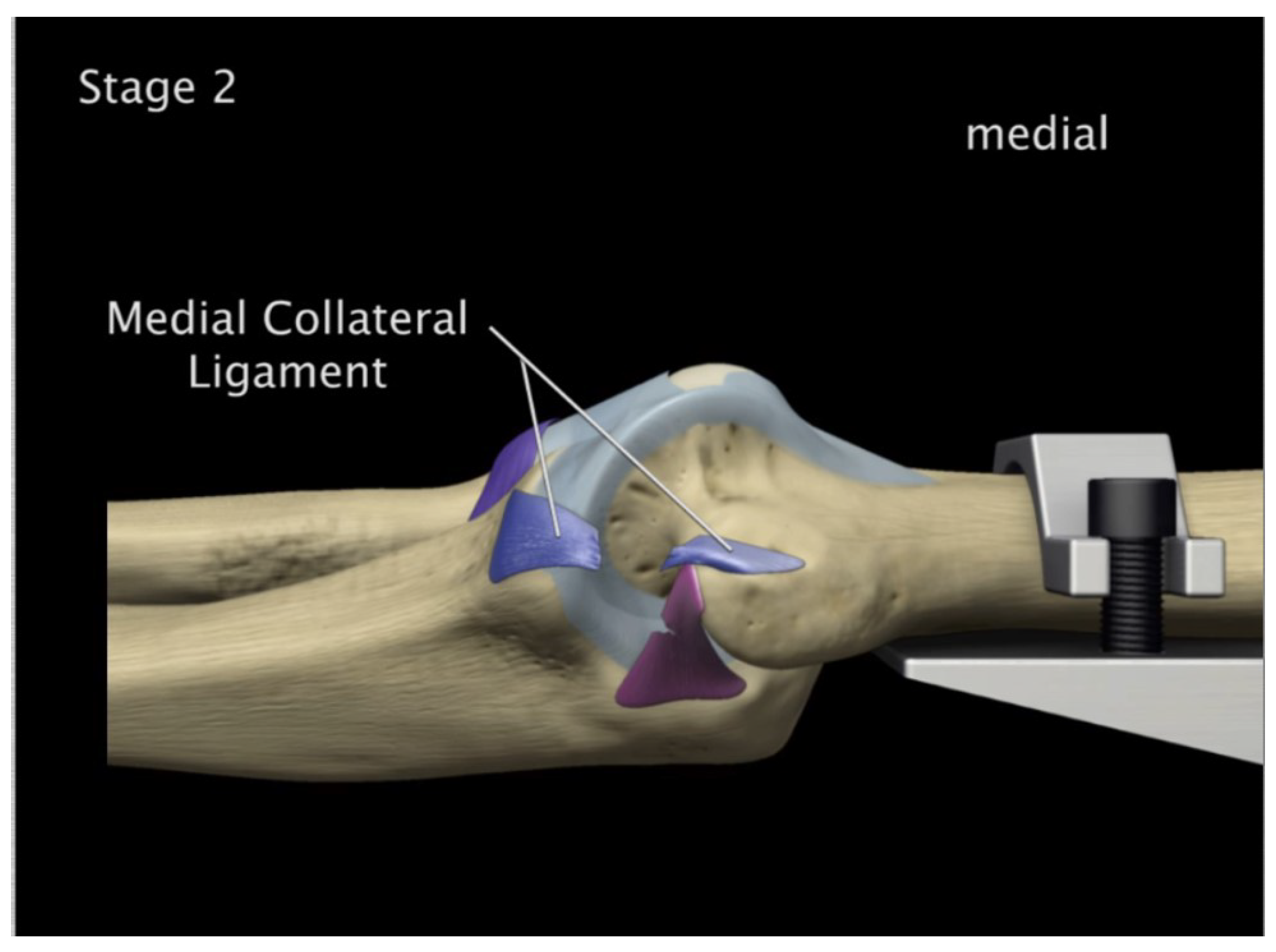
Figure 28.
FE: Displacement of humerus 5° flexion and in pronation
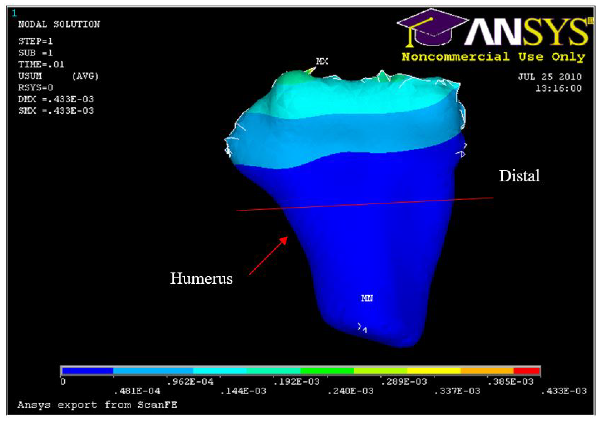
Figure 29.
Experiment Min Distal Humerus Displacement 5° flexion and in pronation
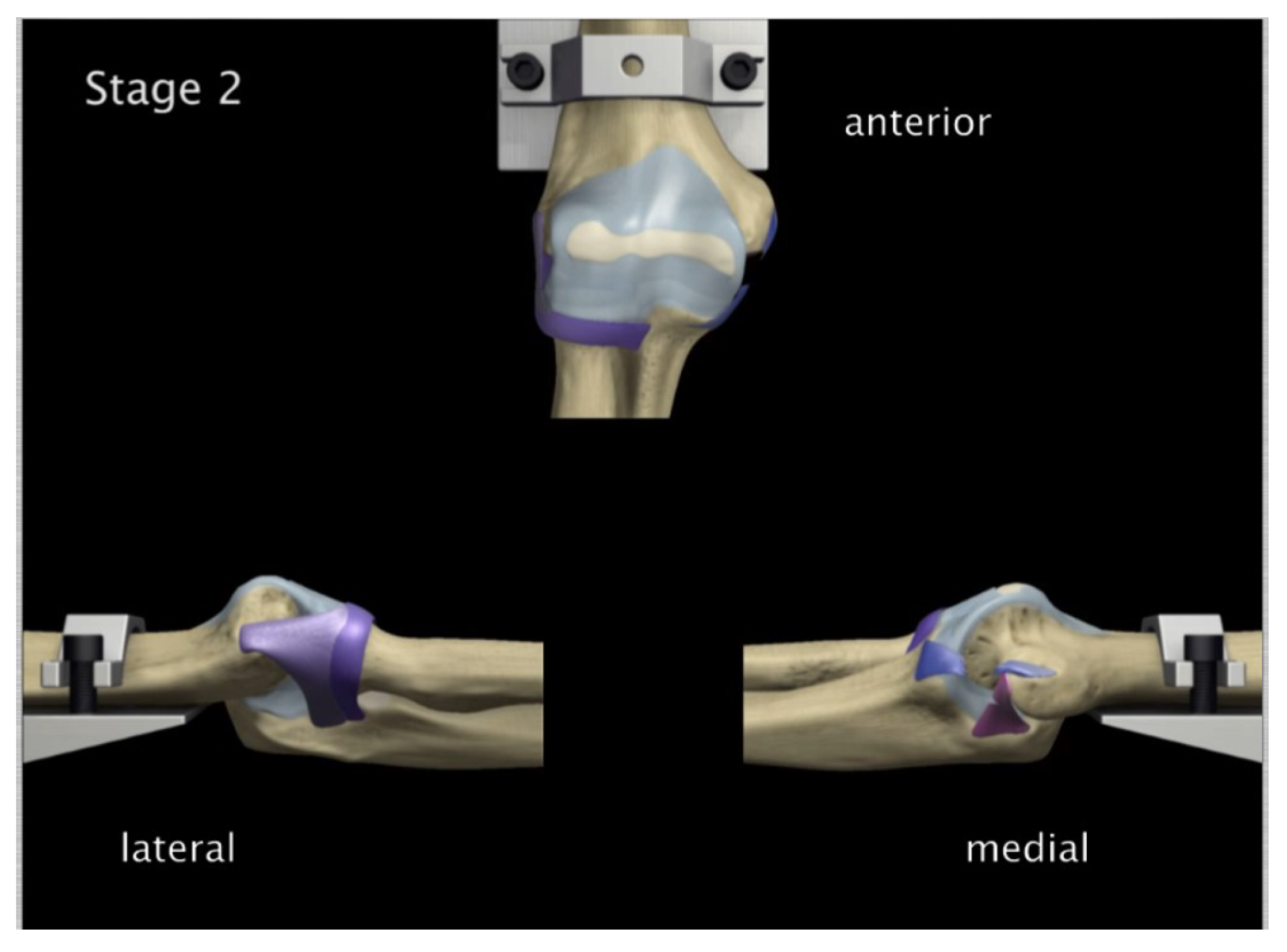
Figure 30.
Anterior capsule tearing at the mid-portion 5° flexion and in pronation
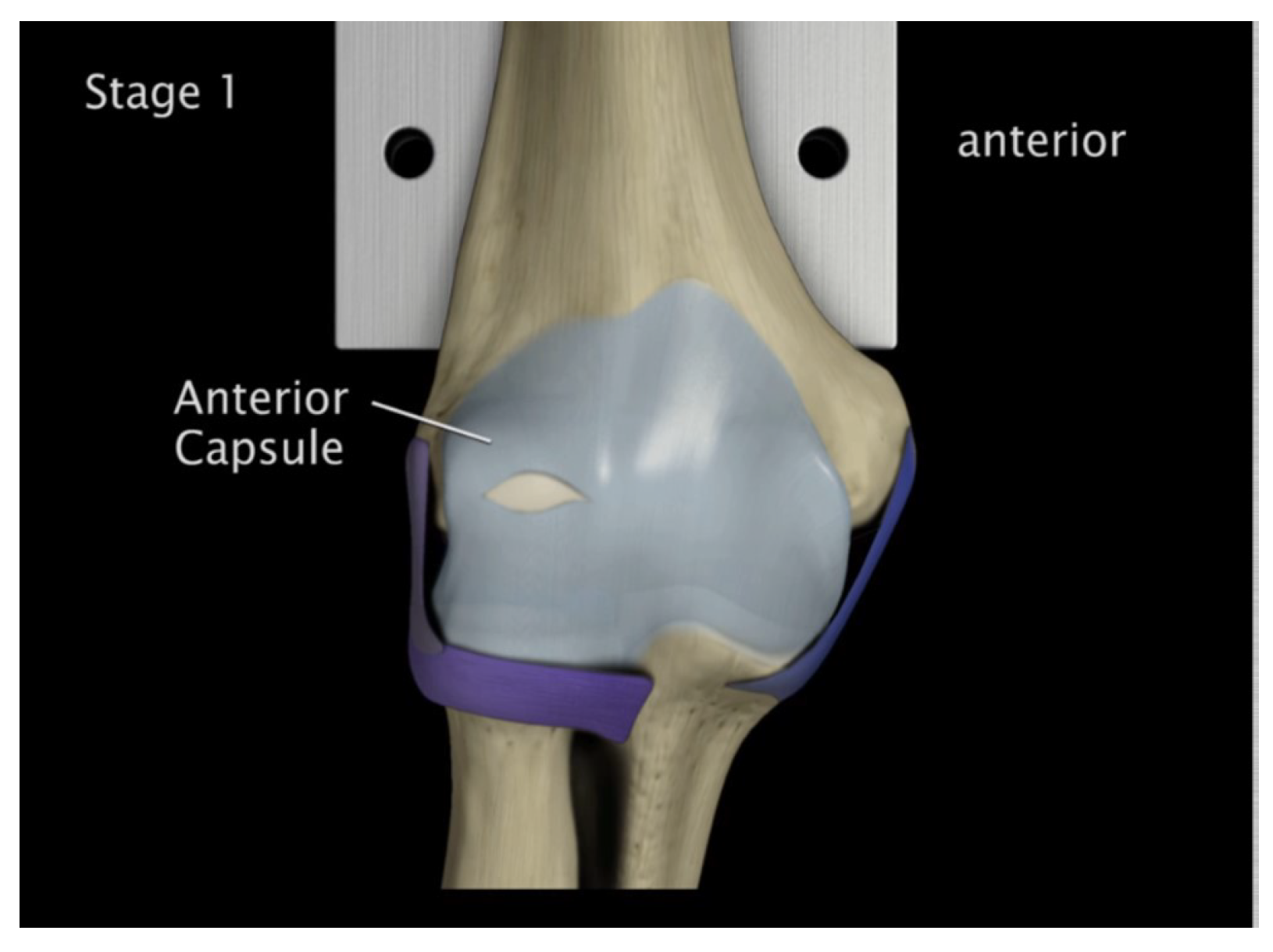
Figure 31.
FE: Nodal Stress at Conoriod Process and Radial Head 5° flexion and in pronation
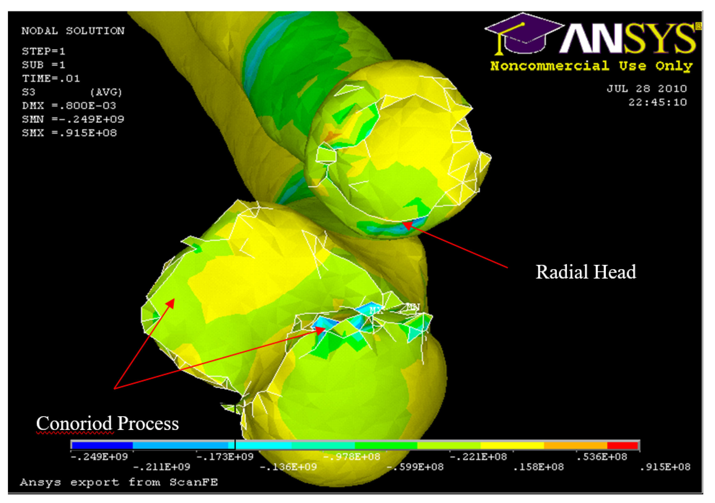
Figure 32.
Experiment: X-ray image of Radial and Conoriod Process Fracture 5° flexion and in pronation
Figure 32.
Experiment: X-ray image of Radial and Conoriod Process Fracture 5° flexion and in pronation
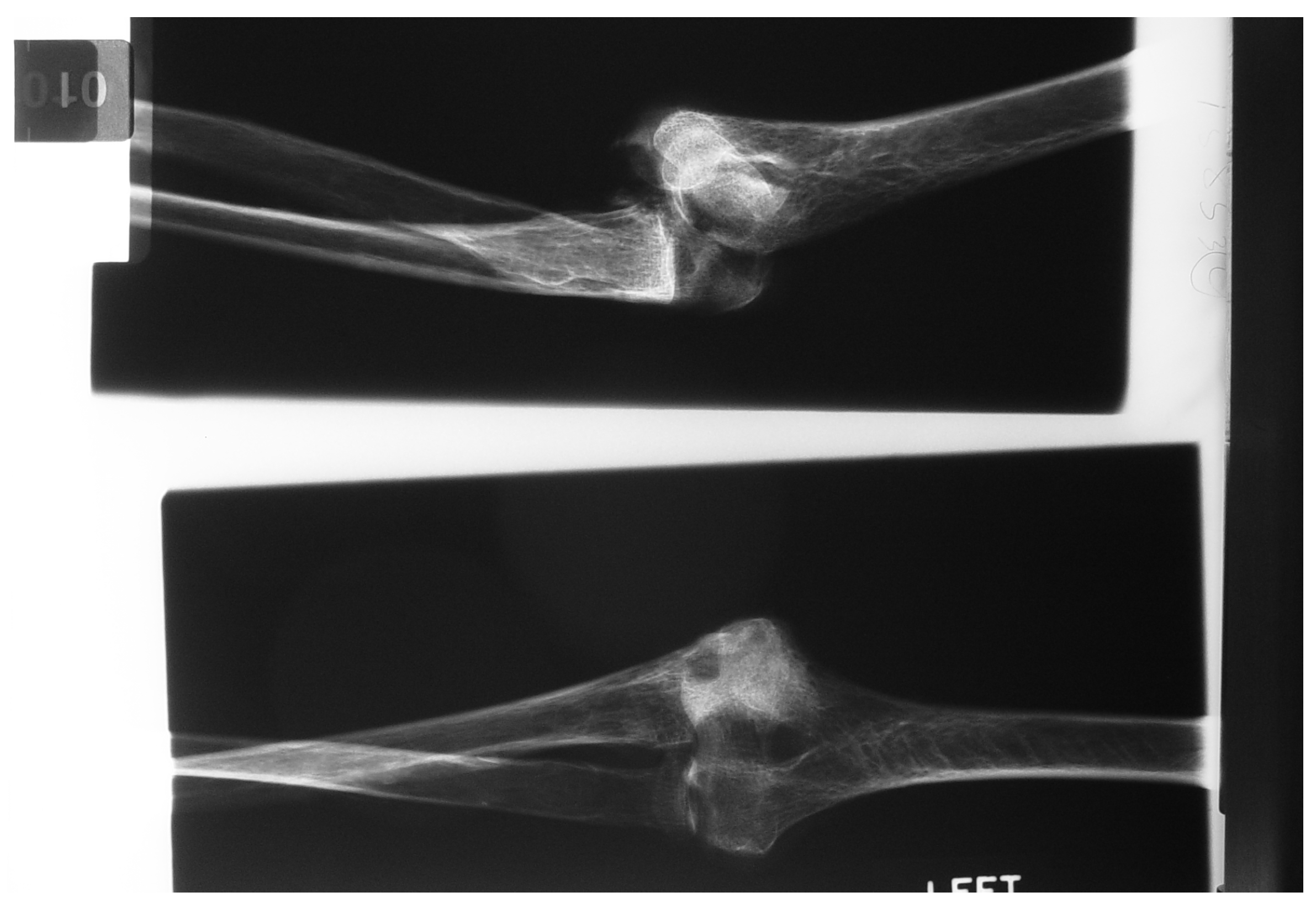
Figure 33.
Posterior Displacement 30° flexion and in pronation
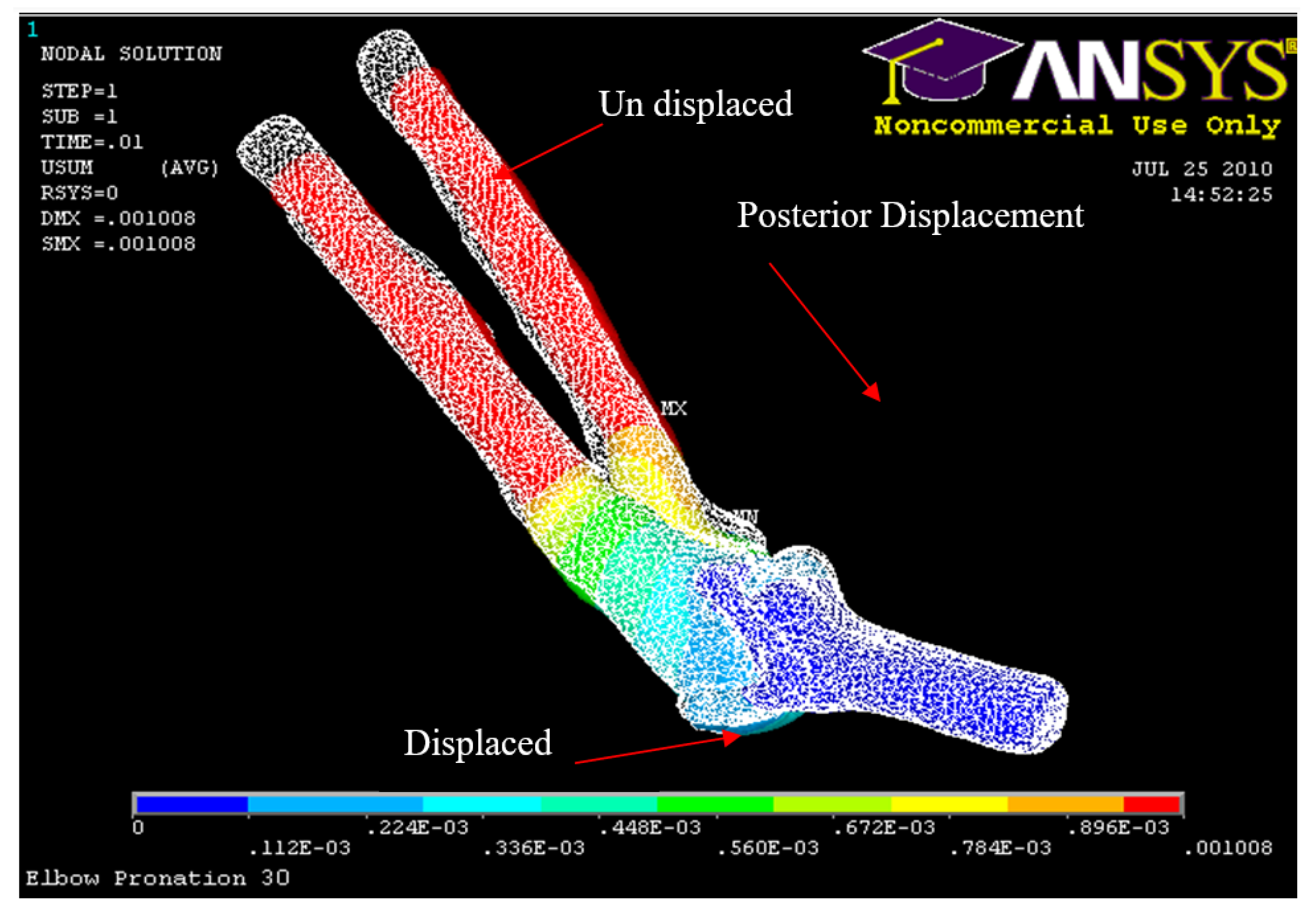
Figure 34.
Posterior Displacement 45° flexion and in pronation
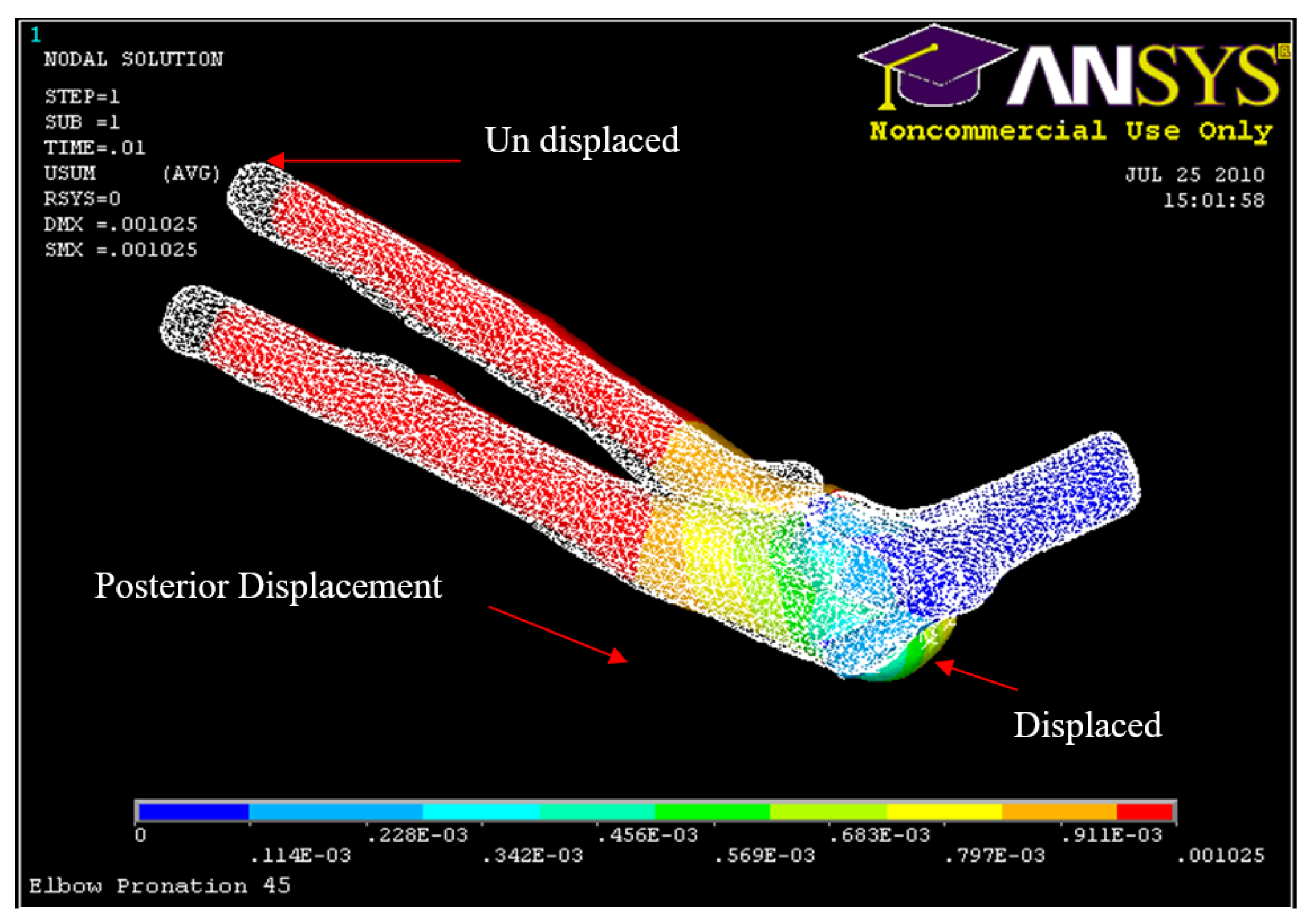
Figure 35.
Posterior Displacement 60° flexion and in pronation
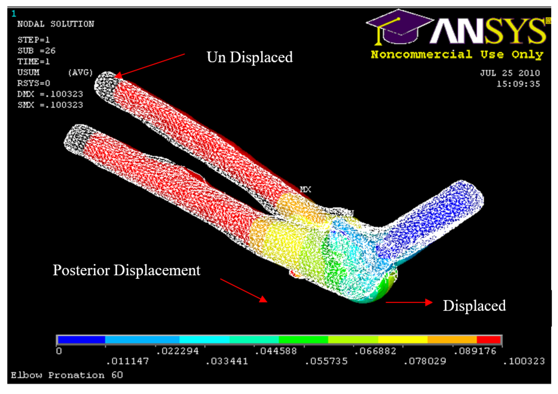
Figure 36.
Posterior Displacement of AMCL, PMCL and RCL 30° flexion and in Pronation
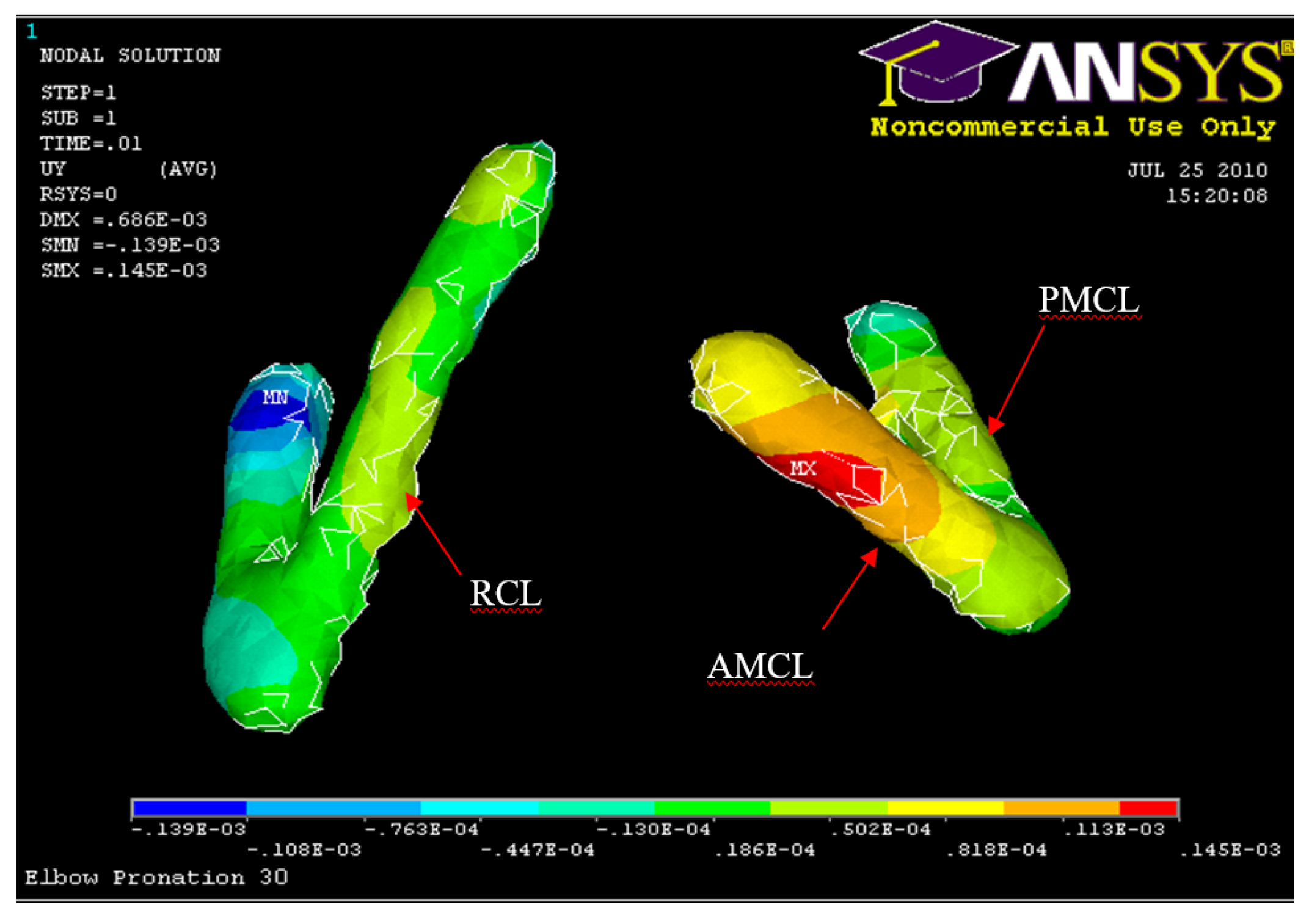
Figure 37.
Posterior Displacement of AMCL, PMCL and RCL 45° flexion and in pronation
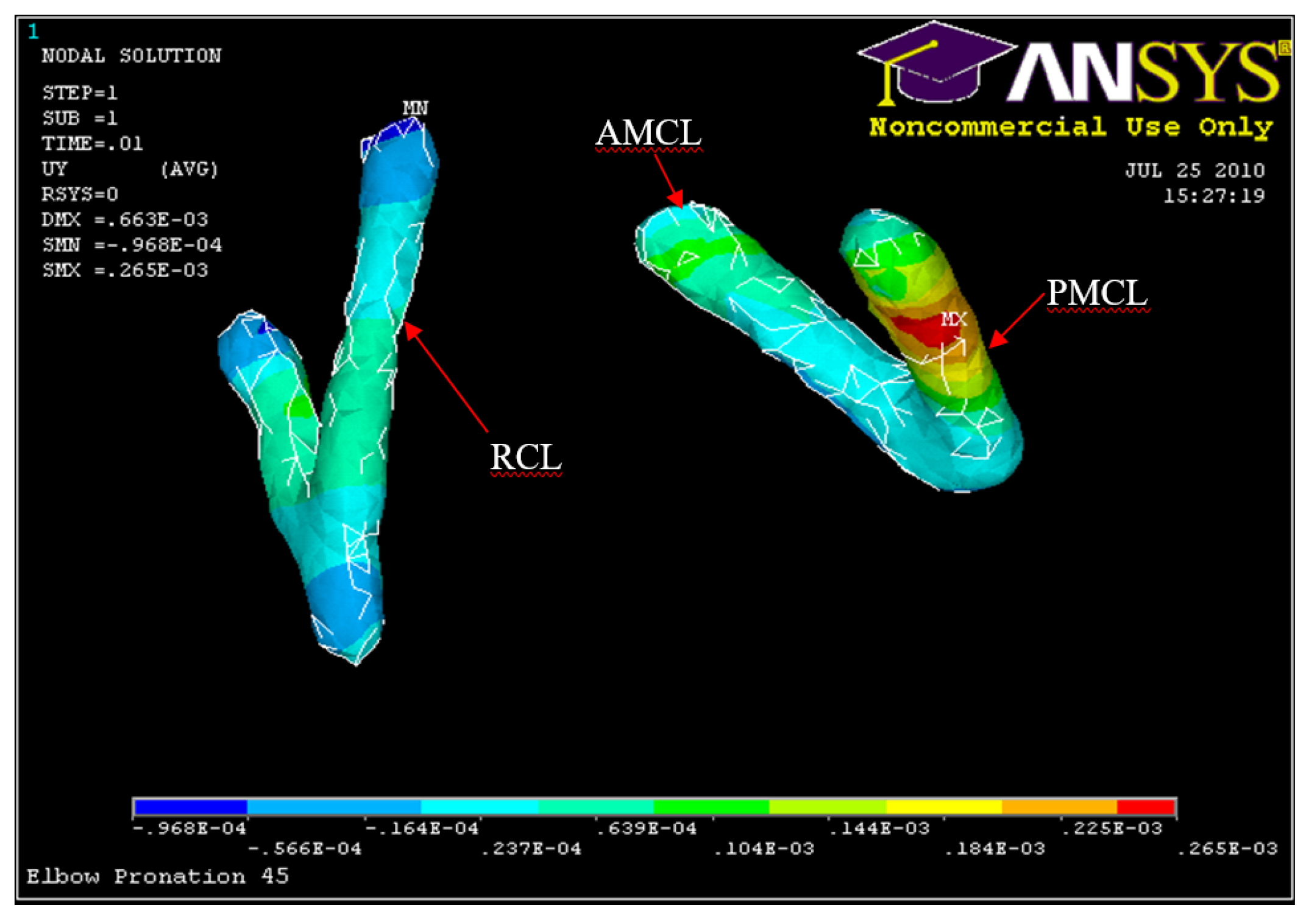
Figure 38.
Posterior Displacement AMCL, PMCL and RCL 60° flexion and in pronation
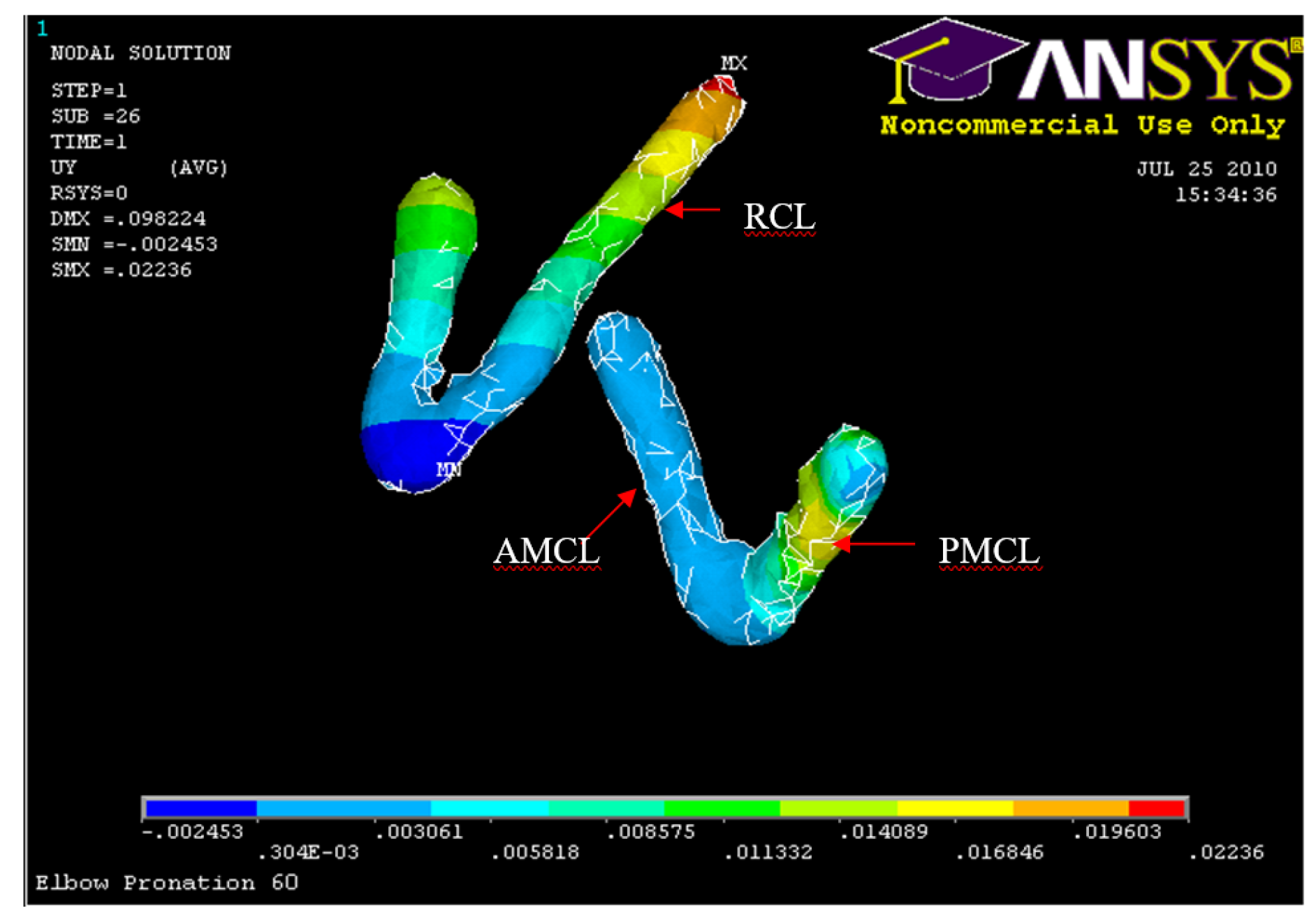
Figure 39.
Humerus Displacement 30° flexion and in pronation
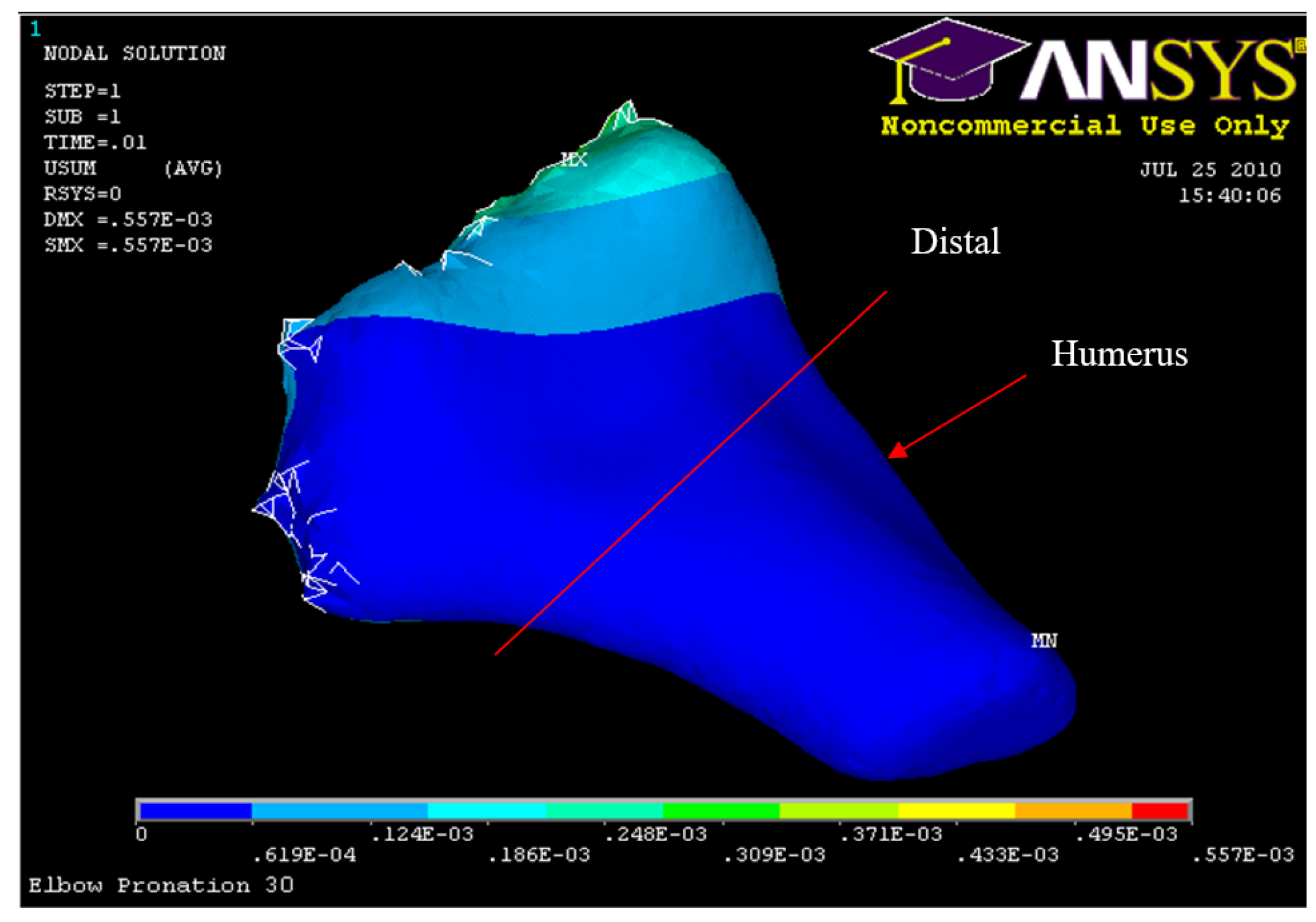
Figure 40.
Humerus Displacement 45° flexion and in pronation
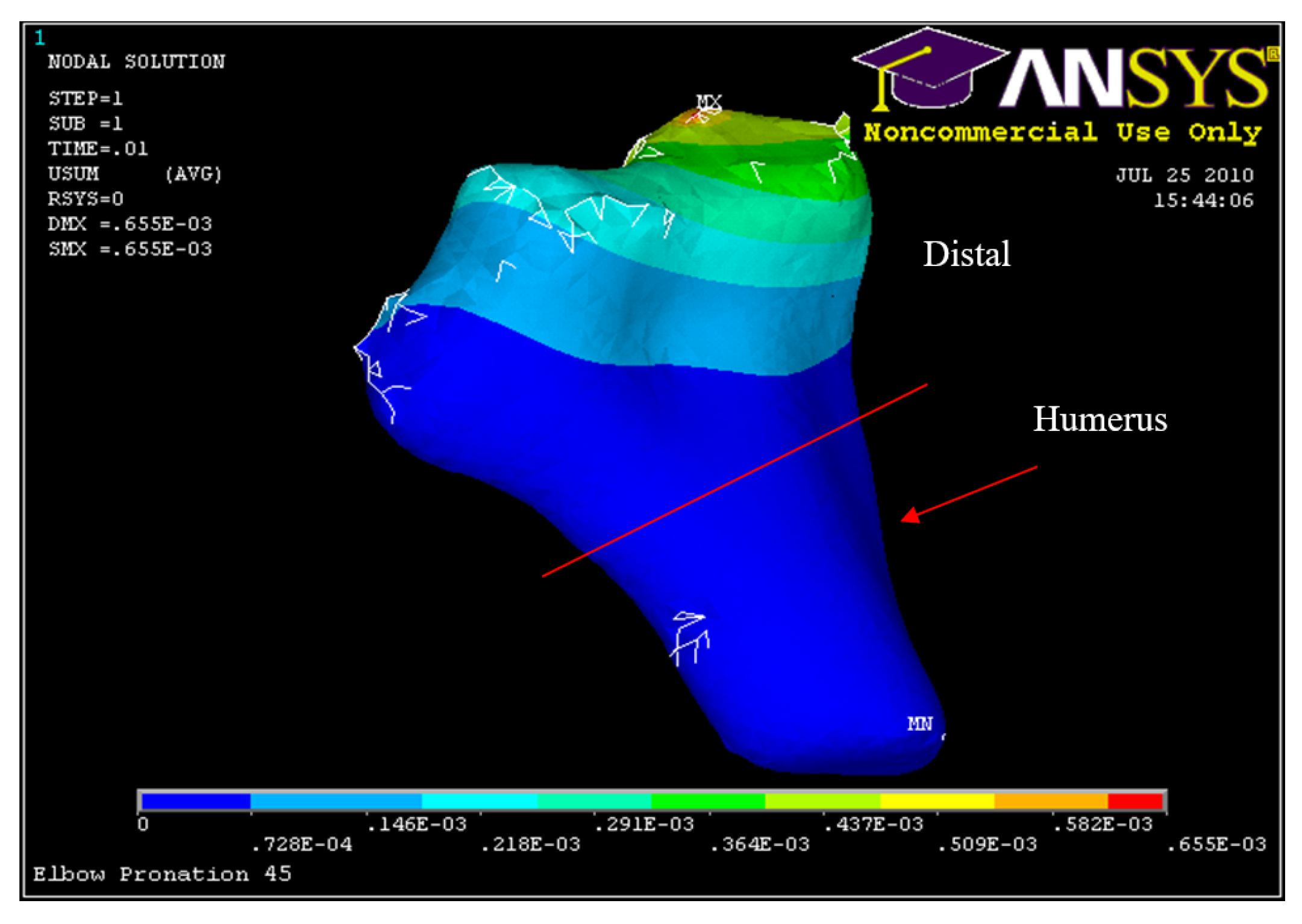
Figure 41.
Humerus Displacement 60° flexion and in pronation
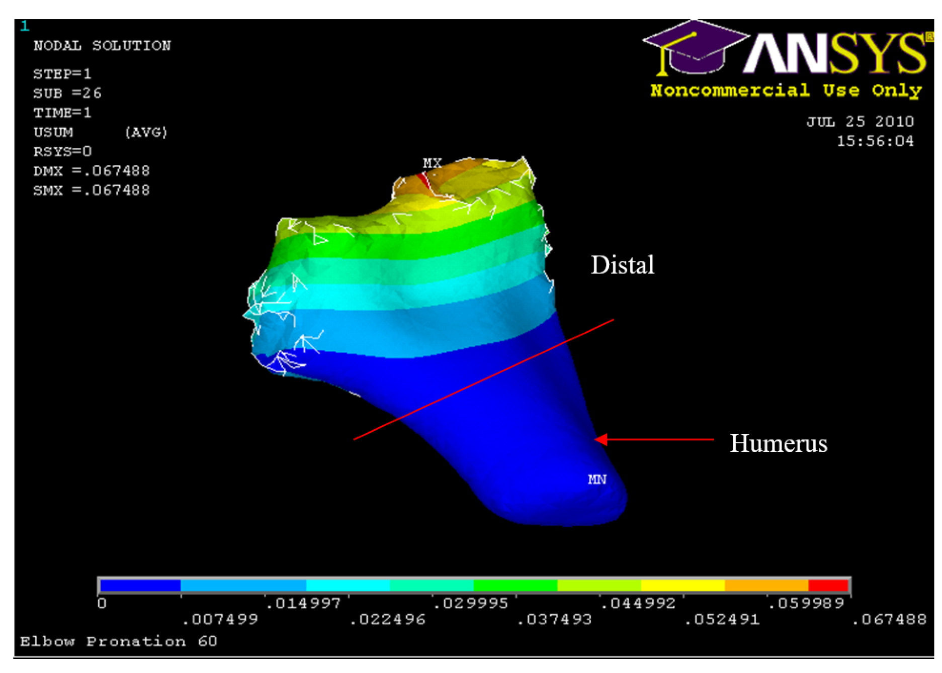
Figure 48.
Posterior Displacement Ulna-Radius
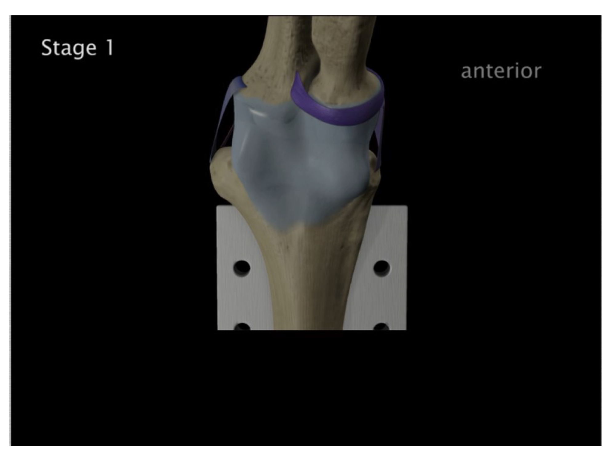
Figure 49.
Radial head & coronoid process fracture
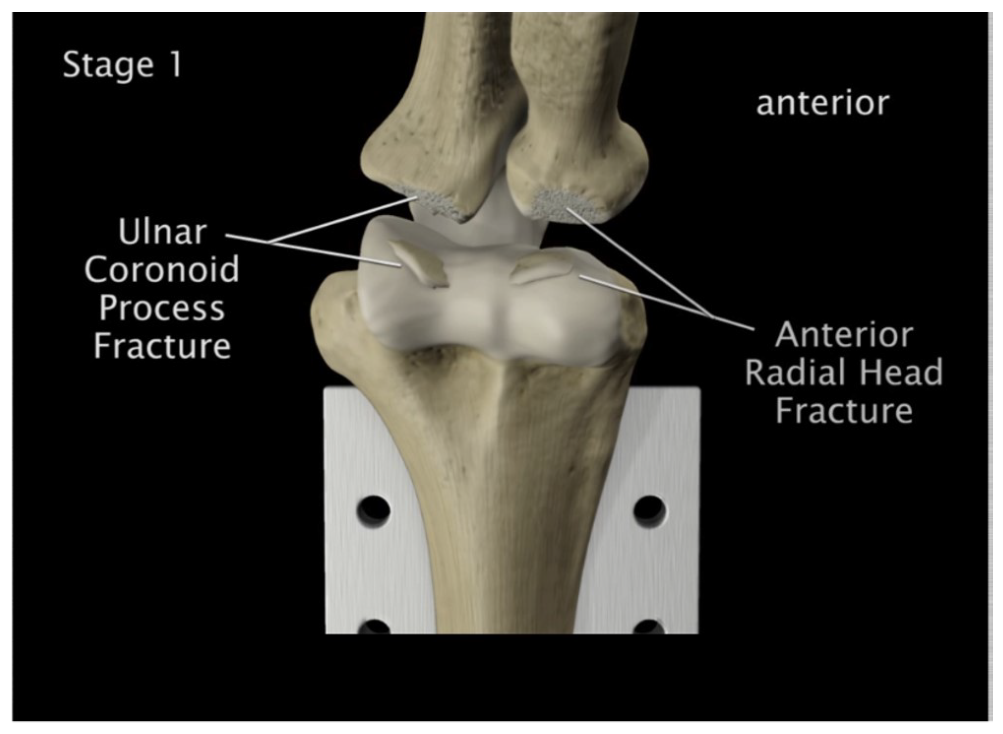
Figure 50.
Medial anterior and lateral posterior capsules were torn
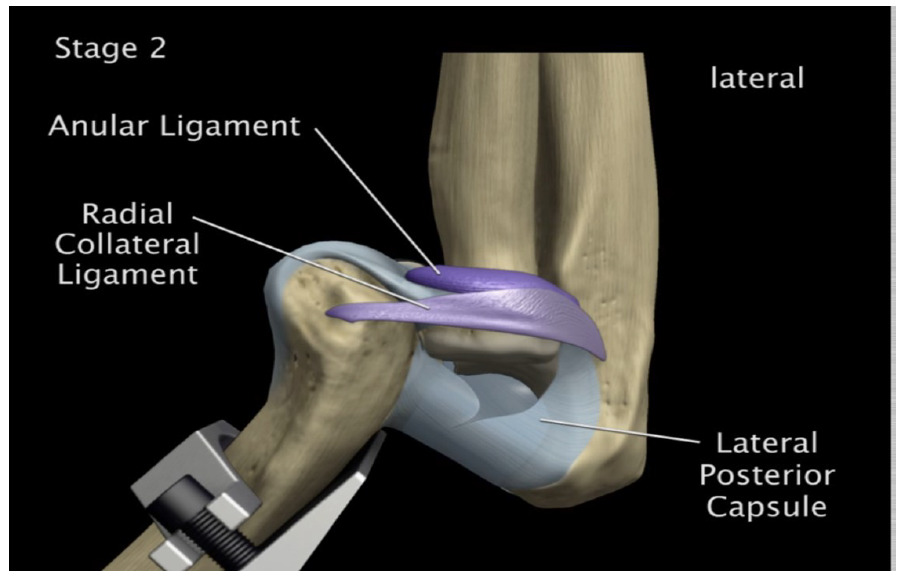
Figure 51.
Medial and lateral tearing of the anterior capsule
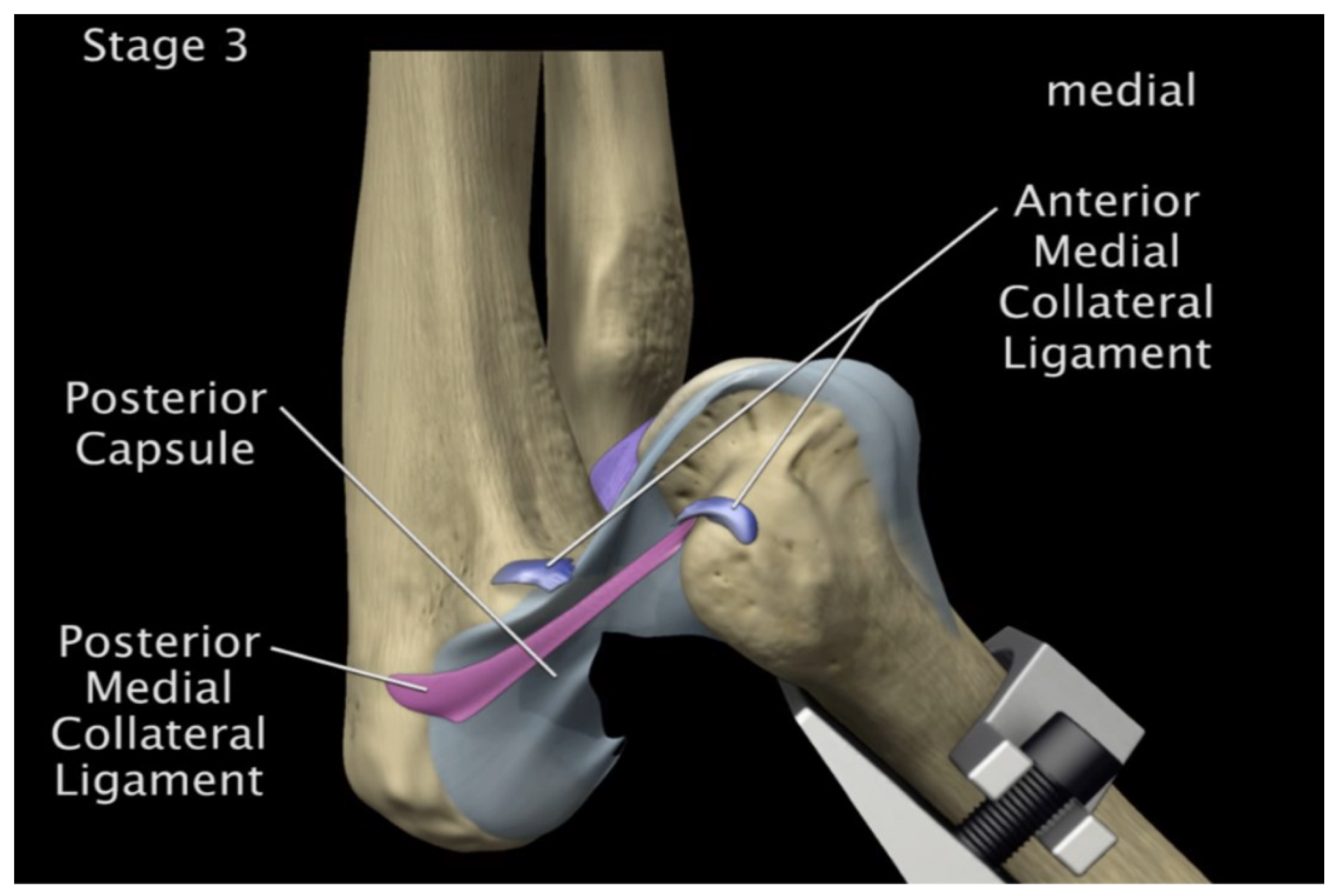
Figure 52.
Posterior displacement of ulna-radius 90° flexion and in pronation
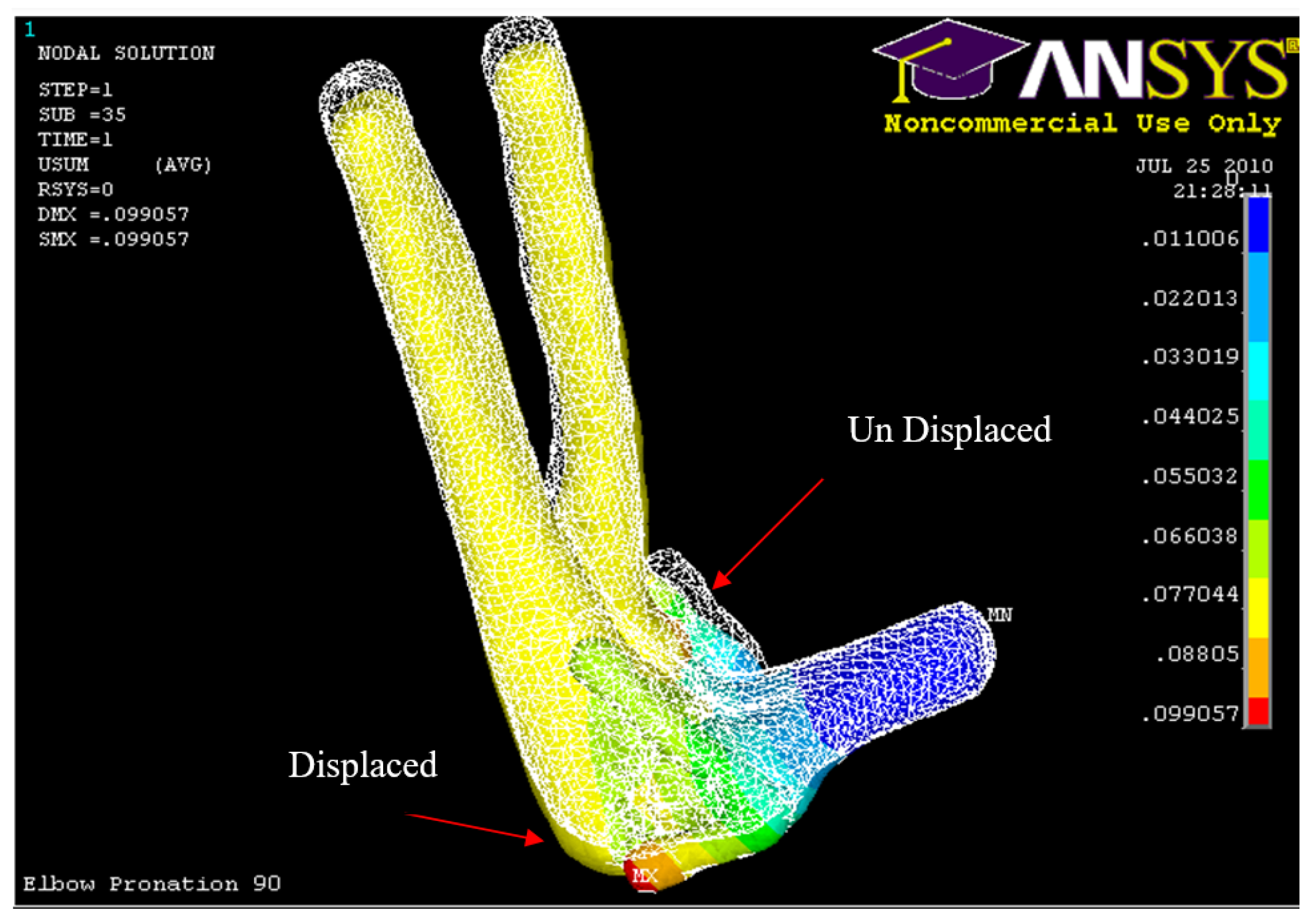
Figure 53.
Posterior Displacement of Humerus 90° flexion and in pronation
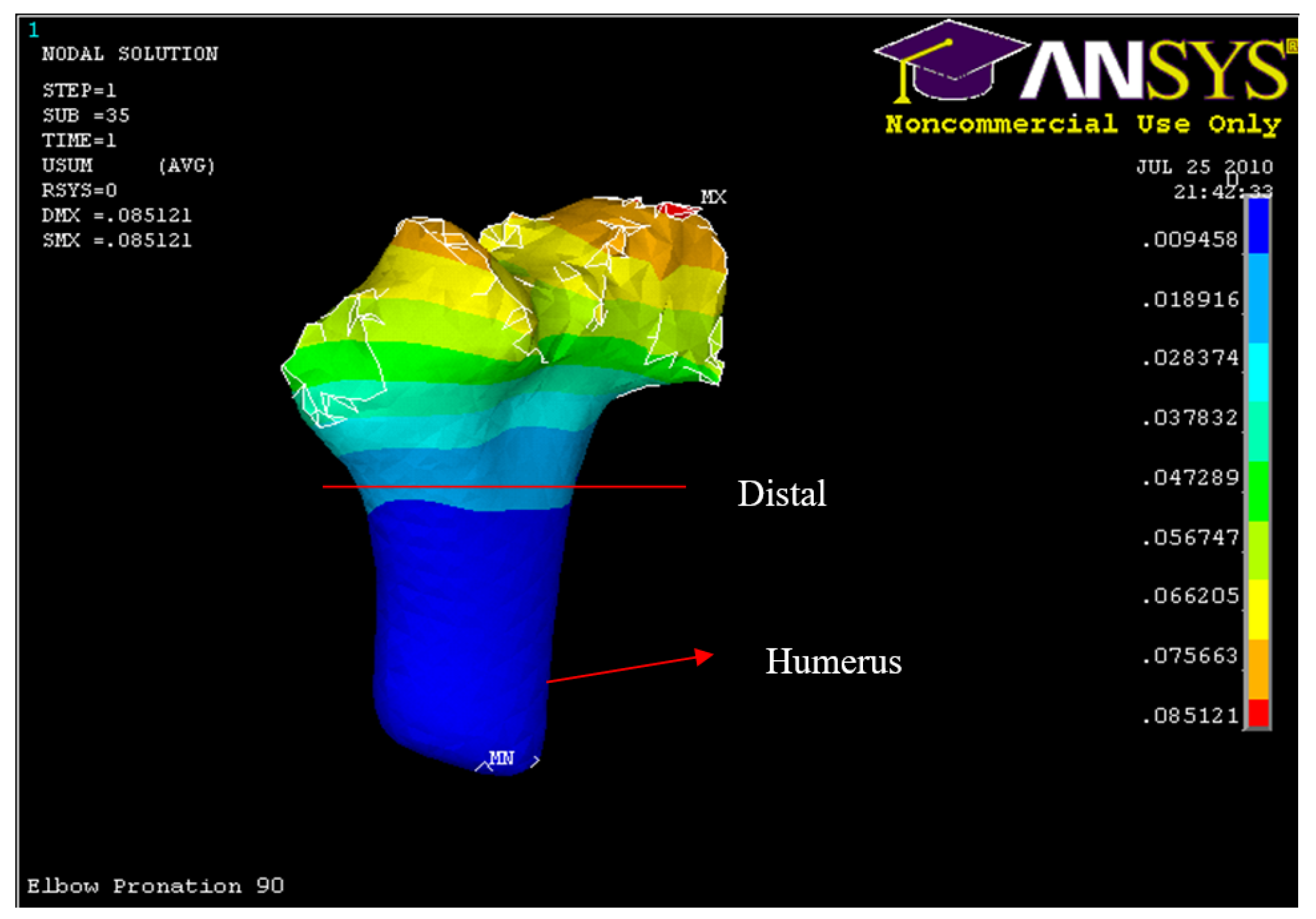
Figure 54.
Posterior Displacement of AMCL, PMCL and RCL in 90° flexion and in pronation
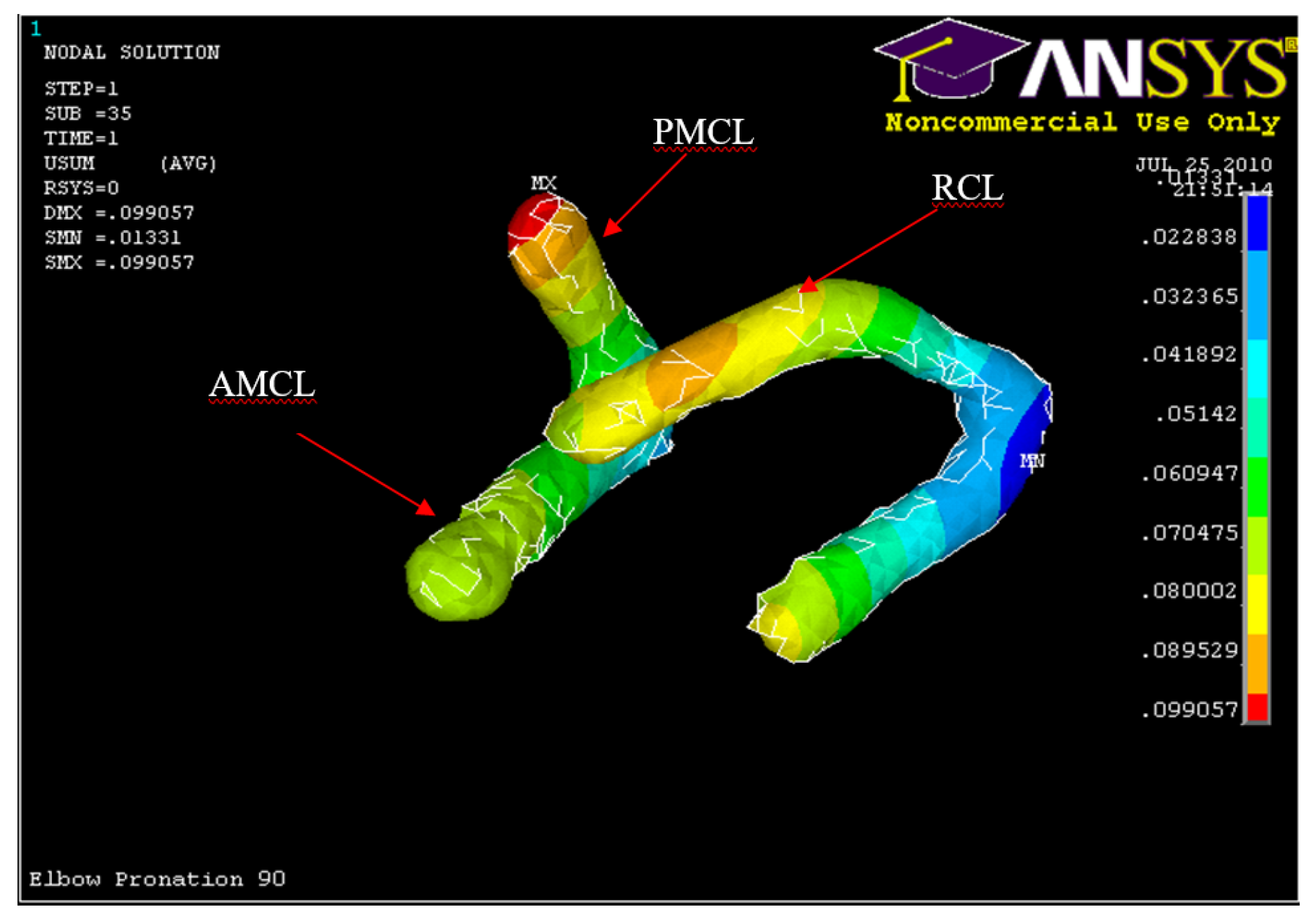
Figure 55.
Humerus distal fracture 90°flexion and in pronation
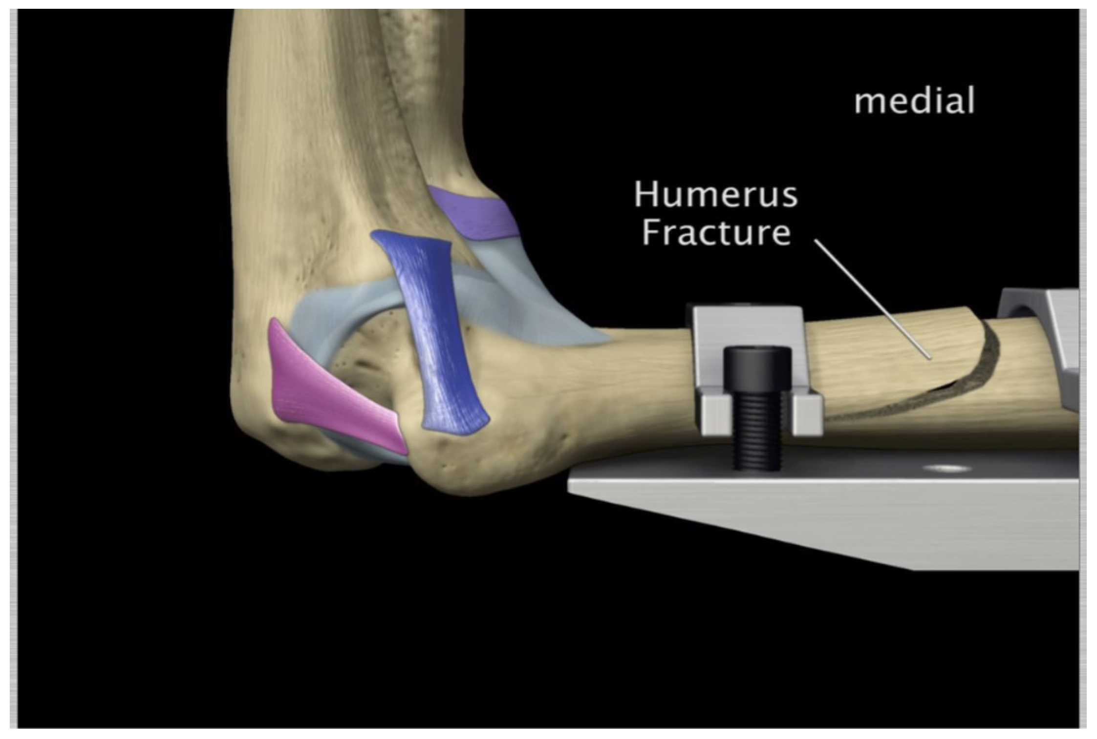
Figure 56.
Nodal Stress at Humerus 90° flexion and in pronation
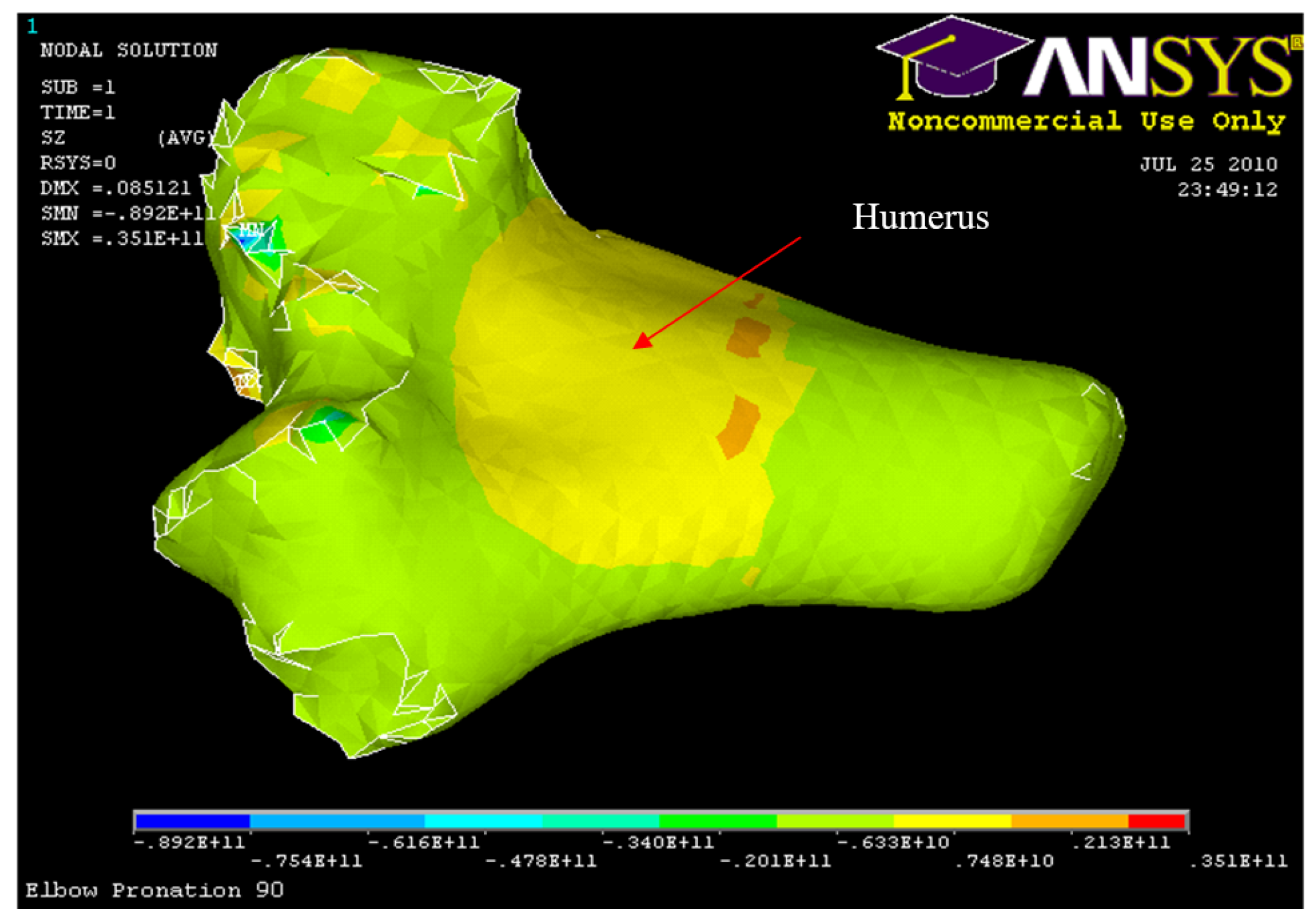
Table 1.
Material Properties of Bone and Soft Tissues
| Material | Young Modulus | Poisson’s | Yield Strength |
|---|---|---|---|
| Cortical Bone | 15-20 GPa | 0.3 | 115-133 MPa |
| Cancellous Bone | 500-1500 MPa | 0.2 | 3-10 MPa |
| Cartilage | 5 MPa | 0.49 | |
| AMCL | 118 MPa | 21 MPa | |
| PMCL | 97 MPa | 19 MPa | |
| RCL | 54 MPa | 16 MPa |
Table 3.
Ligament Mechanical Properties
| AMCL Stress MPa | Strain | PMCL Stress MPa | Strain | RCL Stress MPa | Strain |
|---|---|---|---|---|---|
| 2 | 4 | 0.6 | 4 | 0.6 | 4 |
| 3 | 5 | 1 | 5 | 1 | 5 |
| 4 | 6.5 | 1.5 | 6.5 | 1.4 | 6.5 |
| 5 | 7.9 | 2.2 | 7.9 | 2 | 7.9 |
| 7 | 10 | 3.5 | 10 | 3 | 10 |
| 8 | 11.2 | 4.2 | 11.2 | 3.2 | 11.2 |
| 9 | 12.8 | 5.2 | 12.8 | 3.6 | 12.8 |
| 10 | 13.2 | 5.9 | 13.2 | 3.9 | 13.2 |
| 11.6 | 15 | 7.2 | 15 | 4 | 15 |
| 16.9 | 20 | 12 | 20 | 6 | 20 |
| 22.2 | 25 | 17.4 | 25 | 8.9 | 25 |
| 26.9 | 30 | 25 | 30 | 11 | 30 |
Table 4.
Summary of loading and boundary conditions.
| Group | Components | Displacements (m) | Load (N) |
|---|---|---|---|
| Axial Group | Humerus | Ux = 0, Uy = 0, Uz = 0 | Fx = 0-2000 N |
| Ulna-Radius | Ux = 0.01, Uy = 0, Uz = 0 | ||
| Ligament Attachments | Ux = 0, Uy = 0, Uz = 0 | ||
| Hyper-extension Group | Humerus | Ux = 0, Uy = 0, Uz = 0 | Fz = 0-500 N |
| Ulna-Radius | Ux = 0, Uy = 0, Uz = 0.01 | ||
| Ligament Attachments | Ux = 0, Uy = 0, Uz = 0 |
Table 5.
Human Cadaver Arms Groups Experiments: Characteristics and Average Dislocation Loads Obtained
Table 5.
Human Cadaver Arms Groups Experiments: Characteristics and Average Dislocation Loads Obtained
| Group | Number of elbows | Side | Gender | Characteristics | Average dislocation load |
|---|---|---|---|---|---|
| 1 | 4 | Left | Male | Hyper-extension load 0° flexion | 600 N |
| 2 | 8 | Right | Female | Axial load 5°, 15°, 30°, 45° flexion | 1741 N |
| 4 | Left | ||||
| 2 | Left | Male | 2935 N | ||
| 3 | 2 | Male | Left | Axial load 90° flexion | 2766 N |
Table 6.
Human Cadaver Orientation used in the Experimental Study.
| Gender | Left/right | Orientation | Flexion angle | Number of elbows |
|---|---|---|---|---|
| Male | Left | Supination | 0° | 4 |
| Neutral | 30° | 1 | ||
| Pronation | 45° | 3 | ||
| Female | Left | Supination | 30° | 1 |
| Neutral | 15° | 1 | ||
| 30° | 1 | |||
| Pronation | 5° | 2 | ||
| Right | Pronation | 15° | 4 | |
| 30° | 1 | |||
| 45° | 2 | |||
| Neutral | 30° | 1 |
Table 7.
Max and min nodal displacement for ulna-radius, AMCL, PMCL, LCL and humerus (5° flexion and in pronation)
Table 7.
Max and min nodal displacement for ulna-radius, AMCL, PMCL, LCL and humerus (5° flexion and in pronation)
| Structure | Min vector sum displacement (m) | Max vector sum displacement (m) |
|---|---|---|
| Ulna-Radius | 0.0178 | 0.08 |
| AMCL | 0.00920 | 0.0689 |
| PMCL | 0.0167 | 0.0316 |
| RCL | 0.0 | 0.0615 |
| Humerus | 0.0 | 0.0192 |
Table 8.
Maximum Nodal Stresses occurred at Conoriod Process, Radial Head and Humerus
| Structure | Max compressive/tension stress MPa |
|---|---|
| Coronoid process | -13.6 |
| Radial head | -13.6 |
| Humerus | -17.5 |
Table 9.
List of max, min vector sum displacement of ulna radius (30°, 45°, and 60° flexion and in pronation)
Table 9.
List of max, min vector sum displacement of ulna radius (30°, 45°, and 60° flexion and in pronation)
| Structure | Min vector sum displacement (m) | Max vector sum displacement (m) |
|---|---|---|
| Ulna-Radius (30° Model) | 0.0224 | 0.1 |
| Ulna-Radius (45° Model) | 0.0569 | 0.1 |
| Ulna-Radius (60° Model) | 0.0668 | 0.1 |
Table 10.
List of max, min vector sum displacement of AMCL, PMCL and RCL (30°, 45°, and 60° flexion and in pronation)
Table 10.
List of max, min vector sum displacement of AMCL, PMCL and RCL (30°, 45°, and 60° flexion and in pronation)
| Structure | Min vector sum displacement (m) | Max vector sum displacement (m) |
|---|---|---|
| AMCL (30° Model) | 0.00106 | 0.0145 |
| PMCL (30° Model) | -0.00130 | 0.00502 |
| RCL (30° Model) | 0.00106 | 0.00502 |
| AMCL (45° Model) | 0.00639 | 0.0104 |
| PMCL (45° Model) | 0.00639 | 0.0265 |
| RCL (45° Model) | -0.00968 | 0.00639 |
| AMCL (60° Model) | 0.00857 | 0.00857 |
| PMCL (60° Model) | 0.00857 | 0.0196 |
| RCL (60° Model) | 0.00245 | 0.0223 |
Table 11.
List of max, min vector sum displacement of humerus (30°, 45°, and 60° flexion and in pronation)
Table 11.
List of max, min vector sum displacement of humerus (30°, 45°, and 60° flexion and in pronation)
| Structure | Min vector sum displacement (m) | Max vector sum displacement (m) |
|---|---|---|
| Humerus (30° Model) | 0.0 | 0.0248 |
| Humerus (45° Model) | 0.0 | 0.0437 |
| Humerus (60° Model) | 0.0 | 0.0449 |
Table 13.
Max and Min Nodal Displacement for ulna-radius, AMCL, PMCL, LCL and Humerus 90° flexion and in pronation
Table 13.
Max and Min Nodal Displacement for ulna-radius, AMCL, PMCL, LCL and Humerus 90° flexion and in pronation
| Structure | Min vector sum displacement (m) | Max vector sum displacement (m) |
|---|---|---|
| Ulna-Radius | 0.0330 | 0.0990 |
| AMCL | 0.0323 | 0.0704 |
| PMCL | 0.0323 | 0.0990 |
| RCL | 0.0228 | 0.0895 |
| Humerus | 0.0094 | 0.0756 |
Disclaimer/Publisher’s Note: The statements, opinions and data contained in all publications are solely those of the individual author(s) and contributor(s) and not of MDPI and/or the editor(s). MDPI and/or the editor(s) disclaim responsibility for any injury to people or property resulting from any ideas, methods, instructions or products referred to in the content. |
© 2024 by the authors. Licensee MDPI, Basel, Switzerland. This article is an open access article distributed under the terms and conditions of the Creative Commons Attribution (CC BY) license (http://creativecommons.org/licenses/by/4.0/).
Copyright: This open access article is published under a Creative Commons CC BY 4.0 license, which permit the free download, distribution, and reuse, provided that the author and preprint are cited in any reuse.


