
Submitted:
29 May 2024
Posted:
29 May 2024
You are already at the latest version
Abstract
This work focuses on identifying the most effective machine learning techniques and supervised learning models to precisely estimate power output from Photovoltaic (PV) plants. The performance of various regression models is analyzed by harnessing experimental data, including Random Forest, Support Vector Regression (SVR), Multi-layer Perceptron (MLP), Linear Regressor (LR), Gradient Boosting, and k-Nearest Neighbors (KNN). The methodology applied starts with meticulous data preprocessing steps aimed at ensuring dataset integrity. Following the preprocessing phase, which entails eliminating missing values and outliers using Isolation Feature selection based on a correlation threshold, is performed to identify relevant parameters for accurate prediction in PV systems. Subsequently, Isolation Forest is employed for outlier detection, followed by model training and evaluation using key performance metrics such as Root Mean Squared Error (RMSE), Normalized Root Mean Squared Error (NRMSE), Mean Absolute Error (MAE), and R-squared (R2). Among the array of models evaluated, Random Forest emerges as the top performer, highlighting promising results with an RMSE of 19.413, NRMSE of 0.048% and an R2 score of 0.968. Furthermore, the best-performing model is integrated into a MATLAB application for real-time predictions, thereby enhancing usability and accessibility for a wide range of applications in renewable energy.
Keywords:
PV prediction
; computational modeling
; regression techniques
1. Introduction
In the global pursuit of achieving net-zero emissions, every country has committed to vigorously advancing clean energy initiatives. Among these efforts, PV energy production stands out as a crucial and rapidly developing sustainable energy source, playing a vital role in ensuring the safe, stable, and cost-effective operation of electrical systems. However, the inherently variable nature of PV energy production, influenced by seasonal fluctuations, meteorological conditions, diurnal changes, and solar radiation intensity, presents significant challenges to the reliable integration of large-scale PV grids into the electricity system [1,2,3,4]. Accurate prediction of PV electricity production capacity is therefore essential for developing power generation plans, optimizing power dispatching, and promoting the adoption of new energy sources, ultimately reducing operational costs and enhancing system stability.
Recent efforts in predicting and forecasting PV generation have focused on various modeling approaches, including physical models, statistical analysis models, artificial intelligence (AI) models, and hybrid models [5,6,7].
Physical models rely on geographic and meteorological data to compute PV power, considering factors such as solar radiation, humidity, and temperature. However, modeling complexities arise from the need for detailed geographic and meteorological data specific to PV plants to anticipate production accurately.
On the other hand, statistical models capture historical time series relationships, often utilizing autoregressive moving average models. These autoregressive integrated moving average models, and other similar techniques are known for their simplicity and computational efficiency. Yet, these models are best suited for stable time series data, whereas actual PV data exhibit high variability and significant errors [8]. The advent of smart metering technologies has provided an abundance of real-world data, opening new ways for machine learning and deep learning techniques to enhance data-driven algorithms for PV power generation forecasting. Moreover, the integration of smart meters and data processing capabilities offers novel opportunities to improve the accuracy and reliability of PV production forecasts. By leveraging these advancements, researchers aim to develop more robust and effective prediction models capable of meeting the evolving needs of the renewable energy sector. Due to their potential for extracting representative features and data mining, AI-based models have proven to be more successful than physical and statistical ones [9].
In recent years, conventional machine learning algorithms have emerged as powerful tools for forecasting PV power generation. Demand response, proactive maintenance, energy production, and load predicting are just a few applications where machine learning models are the go-to toolkit for researchers [10]. These models can capture complex nonlinear relationships between various factors influencing power generation and accurately predicting future values [11]. The use of deep learning, nevertheless, can be useful when dealing with time series data.
Auto-Regressive Integrated Moving Averages (ARIMA) methods are effective for instantaneous forecasting of robust time series data. However, artificial neural networks (ANNs) are significantly more powerful than ARIMA models and traditional quantitative approaches, especially for modeling complex interactions [12]. Due to their ability to handle non-linear models, ANNs have increasingly become a popular tool for forecasting time series data in recent years.
In this study, several regression models, including linear regression (LR), support vector regressor (SVM), k-nearest neighbors regressor (KNN), random forest regressor (RF), gradient boosting regressor (GBR), and multilayer perceptron regressor (MLP), were employed for PV power generation forecasting, yielding promising results [13]. The effectiveness of the proposed regression model was compared with existing approaches.
This work makes several key contributions to the field, including advancements in predictive modeling for the renewable energy sector and valuable insights for optimizing PV systems and their management. Techniques such as Pearson and Spearman correlation analysis are used to identify the most pertinent environmental variables. This ensures that only influential factors are considered, boosting both the interpretability and performance of the predictive model. By integrating Isolation Forest for outlier detection during data preprocessing, the method effectively removes anomalies. This enhances the model’s ability to generalize to unseen data and prevents overfitting. Additionally, the use of Randomized Search CV streamlines hyperparameter tuning, with Random Forest emerging as the optimal model choice. Random Forest’s ensemble nature and capacity to capture non-linear relationships make it well-suited for modeling the intricate dynamics of PV system generation. On the other hand, the integration of Python-trained models into a MATLAB interface marks a significant advancement in accurately predicting key parameters for PV systems, such as PV generation, PDC (power at the direct current), VDC (voltage at the direct current), and IDC (current at the direct current). Moreover, this interface goes beyond mere prediction by incorporating calculations to evaluate yield, losses, and performance ratios (PR). This comprehensive assessment capability enables users to conduct thorough analyses system performance and health, providing valuable insights for optimizing efficiency and addressing potential issues.
The paper is structured as follows: In Section 2, we introduce the PV dataset used in the study, outlining the various environmental variables and parameters pertinent to PV systems. In this section, data preprocessing techniques are also described detailing the strategies for refining sensor data, emphasizing the importance of cleaning and normalization for ensuring data accuracy and reliability. The use of Pearson and Spearman correlation analysis to identify significant environmental variables for predictive modeling is also detailed in this section. Additionally, the approach to enhancing regression model performance through outlier detection using Isolation Forest during data preprocessing is discussed. The methodology, providing an overview of the regression models employed for predicting key parameters of PV systems, while outlines our process of hyperparameter tuning using Randomized Search CV and the evaluation metrics utilized to optimize model performance is analyzed too in Section 2. The development of a MATLAB App for Power Prediction, highlighting the integration of Python-trained models and the capabilities of the interface for accurate prediction and system performance evaluation is presented also in Section 2. In Section 3, results obtained are presented showing their implications for the renewable energy sector and suggesting potential avenues for future research. Finally, Section 4 focuses on the discussion of main results obtained.
2. Materials and Methods
The data collected in this study is from a grid-connected, ground-mounted PV system in Ain El-Melh.Algeria. lt is located in the Algerian highlands and serving as the gateway to the vast desert, the site’s coordinates are 34°51″ N and 04°11″ E, with an elevation of 910 meters above sea level.
This PV plant is integrated into Ain El-Melh’s medium voltage network and is part of a substantial 400 MW project overseen by SKTM Company, a subsidiary of Sonelgaz. Sonelgaz, mandated by the Algerian government for renewable energy development, has implemented 23 PV power plants across the highlands and central regions. The Ain El-Melh plant, boasting a total capacity of 20 MWp, spans across 40 hectares. Key design specifications of this 20 MWp PV facility are detailed in Table 1.
The PV modules are linked to 500 kW inverter cabinets via junction boxes, serving as the primary data source. Data gathering occurred from January 1, 2020, to December 31, 2021, with readings taken every fifteen minutes, resulting in 69,195 data points. This dataset encompasses various parameters such as solar panel temperature, tilt radiation, total radiation, dispersion radiation, direct radiation, wind speed, humidity, pressure, voltage, current, and PV power.
Table 2 shows a summary of environmental and electrical parameters of the PV System.
Table 3 provides the technical specifications of the PV modules utilized within this PV plant.
Data preprocessing is essential when working with real data collected from automatic sensors, as this data often contains errors and inconsistencies. To prepare the data for use with machine learning models, cleaning and organizing techniques are applied. The focus is on correcting minor inconsistencies and removing erroneous or missing data from the monitoring dataset.
One challenge encountered is the presence of empty records, particularly during nighttime (between 9 p.m. and 4 a.m.), when no measurements are collected. While solar irradiation is naturally zero during the night, air temperature data may still be missing. However, the absence of nighttime temperature data is irrelevant since there is no PV power production at that time. Including nighttime data would only add redundant information, increasing model complexity and calculation time without yielding meaningful results. To prevent the negative impact of empty records on learning models, rows containing null data are eliminated. The same procedure is applied to remove duplicated values or incomplete records.
After these preprocessing steps, the database ultimately contains 33,465 samples. To optimize the model’s performance and ensure data homogeneity, the min-max normalization method is employed. This process scales each data point to a range between 0 and 1. The equation for calculating the normalized value for a given value x is:
This normalization technique serves various purposes, including speeding up the optimization process, minimizing disparities between data values, removing dimensional influences, and reducing computational requirements.
The analysis examined correlation factors to ascertain the relationships among PDC and individual weather factors. The correlation coefficient, denoted as r, indicates the degree of association between two variables, and , is expressed as follows [15,16,17]:
By applying Equations (3) and (4) to Equation (2), the following equation can be driven:
where {, } and n are the mean and sample size, respectively, and {,} are the individual sample points indexed by i.
Two methods are used for estimating correlation and correlation coefficients between two variables: Pearson and Spearman. The Pearson method assesses the linear relationship between variables, indicating a proportional change between them. Conversely, the Spearman method evaluates a simple (ordinal or rank) relationship, where variables tend to change together without necessarily being proportional.
This study employed the Pearson correlation method to analyze the relationship between PDC and environmental variables. Figure 1 illustrates the outcomes of this correlation analysis, in the heatmap histograms in the diagonal plots demonstrating the frequency distributions of PDC and environmental data.
The correlation matrix provided offers insights into the relationships between PV power generation, voltage, or current and several environmental variables. Each cell in the matrix presents the correlation coefficient between two variables, ranging from -1 to 1. The sign of the coefficient indicates the direction of the relationship: “+” denotes a positive correlation, and “-” denotes a negative correlation. A higher absolute value of the correlation coefficient signifies a stronger association between the variables [18,19].
Analyzing the correlations, several noteworthy patterns were observed. Variables such as tilt solar radiation, Gdin, total Irradiance, Gtotal and direct solar radiation,Gdirect, exhibit strong positive correlations with PV power generation PDC, indicating that higher values of these environmental factors tend to coincide with increased PV power generation. Conversely, the variable H, representing humidity, demonstrates a notable negative correlation with PV power generation, suggesting that higher humidity levels may lead to decreased PV power output. Additionally, some variables, such as Tp, temperature of pv panel, and Gdisp, dispersed solar radiation, show moderate positive correlations with PV power generation. These correlations imply that temperature and dispersed solar radiation may also play significant roles in influencing PV power generation, albeit to a lesser extent compared to other factors like direct solar radiation Gdirect.
Moreover, certain variables, such as V_V, wind speed, and P, pressure, exhibit weaker correlations with PV power generation, as indicated by their correlation coefficients close to zero. While these variables may still have some influence on PV power generation, their impact appears to be relatively minor compared to other environmental factors.
Overall, this correlation analysis provides valuable insights into how various environmental variables relate to PV power generation. Understanding these relationships can inform decision-making processes related to optimizing PV system performance, forecasting energy production, and designing more efficient renewable energy systems.
After loading the dataset, remove any rows with missing values and eliminate the outliers, the target variable PDC is defined. Then, we compute both Pearson and Spearman correlation coefficients separately with the target variable. The correlation coefficients from both methods by selecting the maximum absolute value were combined. After that, the features whose absolute correlation coefficient with target variable is less than or equal to 0.1 were filtered. This process selects a subset of the original features that meet the correlation criterion. The number of input features remains the same; we do not remove any features from the dataset itself but identify which features are relevant based on the correlation threshold. This approach ensures that significant correlations regardless of the method used are captures. Figure 2 demonstrates feature selection based on correlation threshold for PDC data ensuring the identification of pertinent features crucial for accurate prediction and analysis in PV systems.
Isolation Forest is a popular algorithm used for outlier detection in machine learning. It works by isolating anomalies in the dataset rather than modeling the normal data points. This approach is particularly effective for high-dimensional datasets with complex structures. The main principle behind Isolation Forest is that anomalies are typically rare and have attributes that make them easy to isolate. The algorithm exploits this principle by randomly selecting a feature and then randomly selecting a split value between the maximum and minimum values of that feature. This process is repeated recursively until all data points are isolated or a predefined maximum tree depth is reached. During the isolation process, anomalies are expected to be isolated with fewer splits compared to normal data points. Therefore, the path length to isolate an anomaly is typically shorter than that of a normal data point. By measuring the average path length across multiple isolation trees, Isolation Forest assigns anomaly scores to each data point. Data points with shorter average path lengths are considered more anomalous.
In this work, Isolation Forest is used for outlier detection before training the regression models. Specifically, after loading and preprocessing the dataset, Isolation Forest is applied to detect and remove outliers from the dataset using the Isolation Forest class from the sklearn library. After setting the contamination parameter, representing the expected proportion of outliers in the dataset. Outlier predictions are then used to filter out the outliers from the original dataset, resulting in a cleaned dataset containing only the inlier data points. In Figure 3, we present the distributions of PDC before and after the removal of outliers. The X-axis represents PV generation values, while the Y-axis represents the frequency of occurrence. By comparing the two distributions, we gain insights into how the removal of outliers affects the overall distribution of PV generation values.
Figure 3 allows to compare the distribution of the target variables PDC before and after removing outliers, providing insights into the impact of outlier removal on the data distribution. Isolation Forest, by identifying and removing outliers, effectively isolates anomalous data points that may skew the distribution of the variables. By taking out many data points classified as outliers, Isolation Forest helps ensure that the resulting histograms accurately represent the distribution of normal data points within each bin. This enables a clearer understanding of how the data is distributed and how the removal of outliers affects the overall data distribution [20].
The methodology employed in this study began with thorough data preprocessing steps to ensure the integrity of the dataset. Missing values were addressed through either imputation or removal, and relevant features highly correlated with the target variable, Correlated features were identified using Pearson and Spearman correlation coefficients, and then both sets of correlated features were merged. Additionally, outlier detection and removal were performed using Isolation Forest to enhance the robustness of the models. Subsequently, the data were split into training and testing sets for model evaluation. Following data preprocessing, six regression models were selected for evaluation: k-Nearest Neighbors (KNN) [21], Support Vector Regression (SVR) [22], Random Forest [23], Multi-layer Perceptron (MLP), linear regressor (LR) and Gradient Boosting [24]. Each model was subjected to hyperparameter tuning using randomized search CV which involved optimizing various hyperparameters such as the number of estimators, maximum depth, learning rate, kernel type, activation function, and number of neighbors…. etc.
Once the hyperparameters were tuned, the performance of each model was evaluated using multiple metrics, including Root Mean Squared Error (RMSE), Normalized Root Mean Squared Error (NRMSE), Mean Absolute Error (MAE), and R-squared (R2). These metrics, defined in Equations 6-9, provided insights into the accuracy, precision, and goodness of fit of the models [25,26,27].
Results of the model evaluation were analyzed and compared in order to identify the best-performing model for PV generation prediction. This analysis helped highlight the strengths and weaknesses of each model and facilitated the selection of the most suitable model.
After identifying and selecting the best prediction model based on its performance metrics, the next step involves integrating this model into a MATLAB application. This process typically entails exporting the model, along with any necessary preprocessing steps or feature engineering techniques, specially the normalization process, into a format compatible with MATLAB. Once integrated, the model can be deployed within the MATLAB App after converting it into a desktop application using MATLAB App Designer, allowing users to input relevant data and receive predictions or insights based on the model’s calculations. This seamless integration facilitates real-time or on-demand predictions within the MATLAB environment, enhancing the usability and accessibility of the predictive model for various applications and users.
The methodology framework illustrated in Figure 4 guides the approach used. Initially, data collection and preprocessing is set, which includes database exploration and normalization, followed by the segmentation of the data into training and testing sets. In the modeling phase, the objective is to train the chosen algorithms using the training data until a satisfactory model is obtained. To achieve this goal, a randomized search algorithm to identify the best-Hyperparameters for best performing model is applied. Finally, the last stage entails evaluating the models using testing data, calculating estimation errors, then the best model along with its scaler is saved. Additionally, k-fold cross-validation in the training process with a fold size of 5 to enhance the robustness of the evaluations is incorporated.
Hyperparameters are parameters set before the learning process begins, influencing a model’s performance. Their adjustability directly affects model effectiveness. Finding optimal hyperparameters involves trying various combinations. Over time, several approaches, like Grid Search and Random Search, have emerged for hyperparameter optimization. Grid Search, a traditional method, systematically explores a subset of the hyperparameter space through complete search like the used in previous work [28,29]. It is evaluated using various performance metrics, commonly employing cross-validation on the training data. The Random Search Algorithm, also known as the Monte Carlo method or stochastic algorithm [30], operates by iteratively sampling parameter settings from a specified distribution [31], evaluating the model using cross-validation. In contrast to Grid Search, Random Search does not test all parameter values but samples several settings. Random Search demonstrates more efficient performance than Grid Search, as it avoids allocating excessive trials for less important dimensions to optimize the hyperparameters for the all used models [32]. This research employs hyperparameter tuning through a randomized search algorithm. The Randomized Search CV function from the sci-kit-learn library is implemented for this purpose [33]. The Randomized Search CV function randomly selects hyperparameters and evaluates the results. Evaluation is conducted using cross-validation, where the data is divided into two subsets: the learning process data and the validation data. Thus, this study utilizes 5-fold cross-validation to obtain a robust model. The fundamental concept of cross-validation is to split data into two or more subsets, with one subset being used to train the model and the other subset being used for testing the model’s accuracy. K-fold cross-validation is the most typical kind of cross-validation. The data is randomly partitioned into k-equal subgroups, or folds, for k-fold cross-validation. The model is tested on the last fold after being tested on k-1 folds. This process is repeated k times so that each fold is used as a testing set once. The results from each fold are then averaged to produce an overall performance estimate. Figure 5 presents the Process of the used cross-validation technique with 5-fold cross-validation.
In the realm of predictive analytics for power systems, the fusion of Python-based machine learning models with MATLAB’s versatile application framework (App designer) heralds a new era of efficiency and accuracy. The central focus of this work is the design and implementation of a user-friendly MATLAB application tailored for power prediction tasks. The application interface is created using the intuitive App Designer tool provided by MATLAB, allowing for easy interaction and seamless integration with underlying algorithms. Through the application, users can input relevant data, select prediction parameters, and visualize both measured and predicted results in real-time.
Key features of the developed application include:
Tab-Based Interface: The application is organized into tabs corresponding to different prediction tasks, such as predicting power demand, voltage, and current.
Interactive Controls: Users can interact with various components such as buttons, state buttons, and toggle buttons to initiate prediction tasks and customize parameters.
Visualization Tools: Graphical representations, including UI Axes components, facilitate the visualization of measured and predicted data, aiding in the analysis and interpretation of results.
Export Functionality: The application allows users to export prediction results for further analysis or integration with external systems.
Streamlined Integration: Use the generated Excel file from the PV station directly for real-time prediction without any preprocessing required.
The designed MATLAB app offering a user-friendly interface with distinct tabs catering to various prediction types such as Power Distribution Center (PDC), Voltage Distribution Center (VDC), Current Distribution (IDC), Yield, and Loss calculations is shown in Figure 6.
Each tab in the interface is meticulously crafted with intuitive functionality. It features clear visualization through UI Axes and streamlined operations with buttons for tasks like clearing data, triggering predictions, and exporting results.
Additionally, in the yield tab and loss tab, the following calculations are performed:
Reference Yield: Yr for measured or actual and YR for predicted.
This is the time that the sun must be shining with G0 = 1kW/m² in order to radiate the energy Ht to the PV array of the PV module.
Reference Yield = Ht/G0
Array Yield: Ya for Measured or actual and YA for predicted. It indicates the time that the PV system needs to work at the nominal power of the PV array P0 in order to produce the output DC energy EDC.
Array Efficiency = EDC/P0
Final Yield: Yf for Measured or actual and YF for predicted. It is the time that the PV system needs to operate at the nominal power of the PV array P0 in order to produce the output AC energy EAC.
Final Yield = EAC /P0
System Losses: Ls for Measured or actual and LS for predicted.
System Losses = Array Efficiency - Final Yield
Array Capture losses: Lc for Measured or actual and LC for predicted.
Array Capture losses = Reference Yield - Array Efficiency
Performance ratio: Pr for Measured or actual and PR for predicted.
Performance ratio = (Final Yield/ Reference Yield) ×100
The performance ratio represents the ratio between the effective energy EAC and those that would be generated from an ideal, lossless PV installation assuming a 25°C solar cell temperature with the same radiation level. Figure 7 shows the evaluation of the Performance Ratio and losses.
The “hold on plot” button enables users to maintain the UI axes, allowing for the simultaneous plotting of two or more graphs for comparison purposes enhancing accessibility.
Whether it involves predicting PDC, IDC current, and analyzing VDC voltages, or calculating losses, this MATLAB application allows users to seamlessly integrate machine learning models. This facilitates informed decision-making and optimizes performance in power system management.
3. Results
This section presents the results obtained along with the datasets used, showcasing the prediction outcomes of the PV system generation under various weather conditions. Furthermore, the results obtained from the MATLAB app are depicted in separate visualizations.
These results represent the performance metrics for different regression models across PDC datasets. Figure 8 and Figure 9 show a comparison of the measured and predicted PDC plots using RF.
Figure 10 and Table 4 show the comparative analysis of machine learning algorithms for predicting PV power outputs. As it can be seen in the figure, the Random Forest emerges as a top-performing model across all metrics, boasting an RMSE of 21.02 kW, an NRMSE of 0.048%, an MAE of 7.40 kW and an R2 of 0.968, indicating its superior predictive accuracy and robustness. Gradient Boosting also demonstrates competitive performance, particularly in terms of R2: 0.9524 and MAE: 8.60 kW. Conversely, Linear Regressor exhibits comparatively poorer performance across the board, with an RMSE of 30.26 kW, an NRMSE of 0.0670%, an MAE of 10.51 kW, and an R2 of 0.9104. These findings suggest that for accurate predictions of PV power outputs, leveraging Random Forest or Gradient Boosting models would be most beneficial, offering superior predictive capabilities over alternative algorithms
The same work and methodology used for the PDC dataset is applied for both IDC and VDC. Additionally, for the VDC dataset, a filter to exclude all values where the PV generator was not working for better training performance is included. Table 5 shows the results obtained for PDC, IDC, and VDC datasets, presenting various metrics and relevant parameters. The results presented in Figure 11 and Figure 12 pertain to the Random Forest predictions across the test datasets for IDC and VDC respectively.
Figure 13 shows the comparison between actual and predicted values for VDC by using RF. The same information is presented in Figure 14 for IDC.
The results obtained from the MATLAB app, utilizing the random forest regressor trained models for prediction under different weather conditions for PDC, IDC and VDC respectively, are depicted in Figure 15, Figure 16 and Figure 17 for a cloudy day and in Figure 18, Figure 19 and Figure 20 for as clear day.
The results obtained from the MATLAB application utilize the trained random forest regressor models, demonstrating significant success in predicting PV system generation under various weather conditions.
4. Discussion
The analysis carried out showcases the effectiveness of the Random Forest Regressor model in capturing the intricate relationships between environmental variables and PV system performance. For the PDC dataset, the Random Forest model achieved compelling performance with optimal parameters {‘max_depth’: 20, ‘min_samples_leaf’: 2, ‘min_samples_split’: 2, ‘n_estimators’: 200}, resulting in a best RMSE of 21.02 kW, NRMSE of 0.048%, MAE of 7.40 kW, and an impressive R-squared value of 0.968. Similarly, for IDC prediction, the Random Forest model by using the same parameters yielded promising results with a best RMSE of 24.499 kW, NRMSE of 0.0476, MAE of 8.089 kW, and R2 of 0.957, effectively capturing the complex nature of IDC despite fluctuations influenced by various factors. Additionally, for the VDC dataset, the Random Forest model, optimized with {‘max_depth’: 30, ‘min_samples_leaf’: 2, ‘min_samples_split’: 2, ‘n_estimators’: 150}, exhibited superior performance, achieving an RMSE of 11.691 kW, NRMSE of 0.060%, MAE of 7.424 kW, and R2 of 0.953. The analysis carried out revealed that each regression model exhibited varying degrees of performance. The Random Forest model demonstrated competitive performance, with low RMSE, NRMSE and MAE, along with a high R2 score. The SVR also showed promising results, particularly with certain kernel types and regularization parameters. MLP exhibited flexibility with different activation functions and hidden layer sizes but required careful tuning to avoid overfitting. Gradient Boosting and k-Nearest Neighbors showed moderate performance but may benefit from further optimization or feature engineering.
When considering the utilization of Machine Learning for PV power estimation, it’s valuable to compare results with previous studies in the literature. For instance, in [34], a season-customized Artificial Neural Network (ANN) was proposed to forecast the PV power of a system in Italy, achieving an average Mean Absolute Error (MAE) of 17 W. Similarly, the work in [35] reported average MAE values of 33.63 W for Support Vector Regression (SVR) and 50.69 W for ANN estimation of PV power output in Malaysia.
Furthermore, various methodologies have been employed to identify relevant features crucial for accurate prediction. One such approach integrated correlation heatmaps with Bayesian optimization techniques, yielding a R-squared of 0.8917 when utilizing Long Short-Term Memory (LSTM) models with a diverse set of 41 features [36]. Another study utilized wavelet transformation-based decomposition techniques in conjunction with a range of regression models, including WT-LSTM, LSTM, Ridge regression, Lasso regression, and elastic-net regression, achieving a high R-squared of 0.9505 [37]. Moreover, in a separate study, tree-based feature importance and principal component analysis were employed, with ANN and random forest models [38]. This research emphasized the significance of temperature, humidity, day, and time in predicting PV output, resulting in a R-squared of 0.9355. Additionally, traditional regression models such as Linear Regression, SVR, K-Nearest Neighbors Regression, Decision Tree Regression, Random Forest Regression, Multi-layer Perceptron, and Gradient Boosting Regression were assessed using Pearson’s correlation and heatmap analyses, considering factors like hour, power, irradiance, wind speed, ambient temperature, and panel temperature. Among these models, Random Forest Regression demonstrated the highest R-squared of 0.96, highlighting its effectiveness in predicting PV output power. These findings underscore the importance of feature selection methodologies in capturing pertinent features crucial for accurate prediction and analysis in PV systems [43].
On the other hand, Figure 15, Figure 16, Figure 17, Figure 18, Figure 19 and Figure 20 vividly illustrate the predictive outcomes for two distinct days: one characterized by cloudy weather and the other by clear skies. One of the notable advantages of the approach lies in the meticulous selection of relevant features, achieved through Pearson and Spearman correlation analyses. By computing both Pearson and Spearman correlation coefficients between each environmental variable and the target PV system generation, the method ensures a comprehensive understanding of their relationships. This approach enhances model interpretability and performance by incorporating both linear and monotonic correlations, capturing various aspects of the data’s behavior. Additionally, the integration of Isolation Forest for outlier detection enables robust data preprocessing, effectively filtering out anomalies and improving model generalization. Moreover, the implementation of Randomized Search CV facilitates efficient hyperparameter tuning, with Random Forest emerging as the best-performing model. Random Forest’s ensemble nature and ability to handle non-linear relationships make it particularly adept at capturing the complex dynamics of PV system generation. Its versatility, scalability, and resilience to overfitting further underscore its suitability for this application. By seamlessly integrating the trained Random Forest model into the MATLAB App, users can efficiently manage PV systems, leveraging accurate predictions to optimize resource allocation and decision-making.
5. Conclusions
This study has demonstrated the efficiency of employing machine learning techniques for accurate prediction of PV power generation. Through meticulous data preprocessing, feature selection, and model evaluation, Random Forest is identified as the top-performing model for estimating power output from PV plants located in Algeria. Leveraging historical data and computational methods, our approach not only achieves impressive performance metrics such as a low RMSE of 19.413 and high R-squared value of 0.968 but also offers valuable insights into the significance of feature selection and outlier detection in enhancing prediction accuracy.
Furthermore, in addition to models’ evaluation; the integration of the best-performing model into a MATLAB application for real-time predictions is proposed. This step not only enhances the usability and accessibility of predictive modeling in renewable energy but also lays the groundwork for practical implementation in addressing energy demands and promoting sustainability.
To look for further enhance prediction accuracy and robustness, one potential direction is the exploration of Depp learning and hybrid techniques. Additionally, incorporating more weather data, such as cloud cover, could improve the predictive capabilities of the models, especially in regions with variable weather patterns like Algeria. Furthermore, extending this research to consider the integration of energy storage systems, such as batteries, into the predictive models could facilitate better management of intermittent renewable energy sources like solar power. By forecasting both PV power generation and energy storage levels, operators can optimize energy dispatch strategies and improve grid stability.
In essence, as we move towards a future increasingly reliant on clean energy solutions, the integration of advanced computational methods holds immense promise in revolutionizing the renewable energy sector.
Author Contributions
Conceptualization, A.F.A. and A.C.; methodology, A.F.A.; validation, A.F.A., A.C., S.S., H.O. and S.K.; investigation, A.F.A., S.K., H.O., A.C. and S.S.; resources, A.C.; writing—original draft preparation, A.F.A., A.C., and S.S.; writing—review and editing, A.F.A., S.K., H.O., A.C. and S.S. All authors have read and agreed to the published version of the manuscript.
Funding
This research received no external funding.
Data Availability Statement
Data are contained within the article.
Conflicts of Interest
The authors declare no conflicts of interest.
References
- Wang, F.; Xuan, Z.; Zhen, Z.; Li, K.; Wang, T.; Shi, M. A day-ahead PV power forecasting method based on LSTM-RNN model and time correlation modification under partial daily pattern prediction framework. Energy Convers. Manag. 2020, 212, 112766. [Google Scholar] [CrossRef]
- Luo, X.; Zhang, D. An adaptive deep learning framework for day-ahead forecasting of photovoltaic power generation. Sustain. Energy Technol. Assess. 2022, 52, 102326. [Google Scholar] [CrossRef]
- Ahmed, R.; Sreeram, V.; Togneri, R.; Datta, A.; Arif, M.D. Computationally expedient Photovoltaic power Forecasting: A LSTM ensemble method augmented with adaptive weighting and data segmentation technique. Energy Convers. Manag. 2022, 258, 115563. [Google Scholar] [CrossRef]
- Woyte, A.; Van Thong, V.; Belmans, R.; Nijs, J. Voltage fluctuations on distribution level introduced by photovoltaic systems. IEEE Trans. Energy Conv. 2006, 21, 202–209. [Google Scholar] [CrossRef]
- Chen, J.; Zhang, N.; Liu, G.; Guo, L.; Li, J. Photovoltaic short-term output power forecasting based on EOSSA-ELM. Renew. Energy 2022, 40, 890–898. [Google Scholar]
- Mayer, M.J.; Grof, G. Extensive comparison of physical models for photovoltaic power forecasting. Applied Energy 2020, 283, 116239. [Google Scholar] [CrossRef]
- Shi, J.; Lee, W.J.; Liu, Y.Q.; Yang, Y.P.; Wang, P. Forecasting power output of photovoltaic systems based on weather classification and support vector machines. IEEE Trans. Ind. Appl. 2012, 48, 1064–1069. [Google Scholar] [CrossRef]
- Singh, S.N.; Mohapatra, A. Repeated wavelet transform based ARIMA model for very short-term wind speed forecasting. Renew. Energy 2019, 136, 758–768. [Google Scholar]
- Daut, M.A.M.; Hassan, M.Y.; Abdullah, H.; Rahman, H.A.; Abdullah, M.P.; Hussin, F. Building electrical energy consumption forecasting analysis using conventional and artificial intelligence methods: A review. Renew. Sustain. Energy Rev. 2017, 70, 1108–1118. [Google Scholar] [CrossRef]
- Zhou, H.; Rao, M.; Chuang, K.T. Artificial intelligence approach to energy management and control in the HVAC process: An evaluation, development and discussion. Dev. Chem. Eng. Miner. Process. 1993, 1, 42–51. [Google Scholar] [CrossRef]
- De Benedetti, M.; Leonardi, F.; Messina, F.; Santoro, C.; Vasilakos, A. Anomaly detection and predictive maintenance for photovoltaic systems. Neurocomputing 2018, 310, 59–68. [Google Scholar] [CrossRef]
- Elsaraiti, M.; Merabet, A. A comparative analysis of the arima and lstm predictive models and their effectiveness for predicting wind speed. Energies 2021, 14, 6782. [Google Scholar] [CrossRef]
- Lee, S.; Nengroo, S.H.; Jin, H.; Doh, Y.; Lee, C.; Heo, T.; Har, D. Anomaly detection of smart metering system for power management with battery storage system/electric vehicle. ETRI J. 2023, 45, 650–665. [Google Scholar] [CrossRef]
- Shi, J.; Lee, W.J.; Liu, Y.Q.; Yang, Y.P.; Wang, P. Forecasting power output of photovoltaic systems based on weather classification and support vector machines. IEEE Trans. Ind. Appl. 2012, 48, 1064–1069. [Google Scholar] [CrossRef]
- Spearman, C. ; The proof and measurement of association between two things. Amer. J. Psychol. 1904, 15, 1, 72–101. [Google Scholar] [CrossRef]
- Kuei Lin, L. ; Concordance correlation coefficient to evaluate repro-ducibility. Biometrics 1989, 45, 1, 255–268. [Google Scholar]
- Best, D.J.; Roberts, D.E. ; Algorithm AS 89: The upper tail proba-bilities of Spearman’s ρ. J. Roy. Statist. Ser. C (Appl. Statist.) 1975, 24, 377–379. [Google Scholar]
- Revelle, W. Psych v1.8.4, 2018. Available online: https://www.rdocumentation.org/packages/psych/versions/1.8.4/topics/pairs.panels (accessed on 5 May 2024).
- Weisstein, E.W.S. ; Rank correlation, coefficient 1999. Available online: https://mathworld.wolfram.com/SpearmanRankCorrelationCoefficient.html (accessed on 15 May 2024).
- Liu, F.T.; Ting, K.M.; Zhou, Z.H. Isolation-based anomaly detection. ACM Transactions on Knowledge Discovery from Data (TKDD) 2012, 6, 1–39. [Google Scholar] [CrossRef]
- Margoum, S. et al. Prediction of Electrical Power of Ag/Water-Based PVT System Using K-NN Machine Learning Technique. In Proceedings of the International Conference on Digital Technologies and Applications, Fez, Moroco, 27 Jan. 2023.
- Kuriakose, A.M.; Kariyalil, D.P.; Augusthy, M.; Sarath, S.; Jacob, J.; Antony, N.R. ; Comparison of Artificial Neural Network, Linear Regression and Support Vector Machine for Prediction of Solar PV Power. In Proceedings of the 2020 IEEE Pune Section International Conference (PuneCon), Pune, India, 16 December 2020. [Google Scholar]
- Khalyasmaaet, A. al. Prediction of Solar Power Generation Based on Random Forest Regressor Model. In Proceedings of the International Multi-Conference on Engineering, Computer and Information Sciences (SIBIRCON), Novosibirsk, Russia, 21 October 2019. [Google Scholar]
- Gupta, R.; Yadav, A.K.; JHA, S.K.; et al. Predicting global horizontal irradiance of north central region of India via machine learning regressor algorithms. Engineering Applications of Artificial Intelligence 2024, 133, 108426. [Google Scholar] [CrossRef]
- Shah, I.; Iftikhar, H.; Ali, S. Modeling and Forecasting Electricity Demand and Prices: A Comparison of Alternative Approaches. J. Math. 2022, 3581037. [Google Scholar] [CrossRef]
- Shah, I.; Jan, F.; Ali, S. Functional data approach for short-term electricity demand forecasting. Math. Probl. Eng. 2022, 6709779. [Google Scholar] [CrossRef]
- Lisi, F.; Shah, I. Forecasting next-day electricity demand and prices based on functional models. Energy Syst. 2020, 11, 947–979. [Google Scholar] [CrossRef]
- Amiri, A.F.; Oudira, H.; Chouder, A.; Kichou, S. Faults detection and diagnosis of PV systems based on machine learning approach using random forest classifier. Energy Conversion and Management 2024, 301, 118076. [Google Scholar] [CrossRef]
- Amiri, A.F.; Kichou, S.; Oudira, H.; Chouder, A.; Silvestre, S. Fault Detection and Diagnosis of a Photovoltaic System Based on Deep Learning Using the Combination of a Convolutional Neural Network (CNN) and Bidirectional Gated Recurrent Unit (Bi-GRU). Sustainability 2024, 16, 1012. [Google Scholar] [CrossRef]
- Vapnik, V.N. ; Statistical learning theory. Wiley, New York, USA,1998.
- Rojas-Dominguez, L.C.; Padierna, J.M.; Carpio Valadez, H.J. ; Puga-Soberanes and. Fraire, H.J.; Optimal Hyper-Parameter Tuning of SVM Classifiers with Application to Medical Diagnosis I.EEE Access 2018, 6, 7164–7176. [Google Scholar]
- Ramaprakoso. Analisis-Sentimen, GitHub. Available online: https://github.com/ramaprakoso/analisis-sentimen/blob/master/ kamus/acronym.txt. (accessed on 20 March 2024).
- Ahmad, M.; Aftab, S.; Salman, M.; Hameed, N.; Ali, I. and Nawaz, Z. SVM Optimization for Sentiment Analysis. International Journal of Advanced Computer Science and Applications 2018, 9, 393–398. [Google Scholar]
- Radicioni, M.; Lucaferri, V.; De Lia, F.; Laudani, A.; Lo Presti, R.; Lozito, G.M.; Riganti Fulginei, F.; Schioppo, R.; Tucci, M. Power Forecasting of a Photovoltaic Plant Located in ENEA Casaccia Research Center. Energies 2021, 14, 707. [Google Scholar] [CrossRef]
- Das, U.; Tey, K.; Seyedmahmoudian, M.; Idna Idris, M.; Mekhilef, S.; Horan, B.; Stojcevski, A. SVR-Based Model to Forecast PV Power Generation under Different Weather Conditions. Energies 2017, 10, 876. [Google Scholar] [CrossRef]
- Aslam, M.; Lee, S.-J.; Khang, S.-H.; Hong, S. Two-stage attention over LSTM with Bayesian optimization for day-ahead solar power forecasting. IEEE Access 2021, 9, 107387–107398. [Google Scholar] [CrossRef]
- Mishra, M.; Dash, P.B.; Nayak, J.; Naik, B.; Swain, S.K. Deep learning and wavelet transform integrated approach for short-term solar power prediction. Measurement 2020, 166, 108250. [Google Scholar] [CrossRef]
- Munawar, U.; Wang, Z. A framework of using machine learning approaches for short-term solar power forecasting. J. Electr. Eng. Technol. 2020, 15, 561–569. [Google Scholar] [CrossRef]
- Abdullah, B.U.D.; Khanday, S.A.; Islam, N.U.; Lata, S.; Fatima, H.; Nengroo, S.H. Comparative Analysis Using Multiple Regression Models for Forecasting Photovoltaic Power Generation. Energies 2024, 17, 1564. [Google Scholar] [CrossRef]
Figure 1.
The heatmap of the outcomes of this correlation analysis.
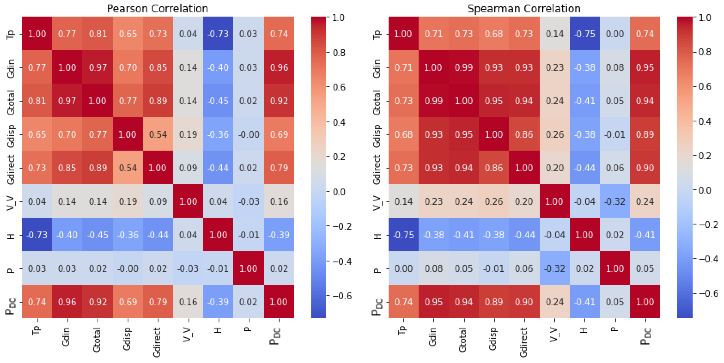
Figure 2.
The Feature Selection based on Correlation Threshold for PDC.
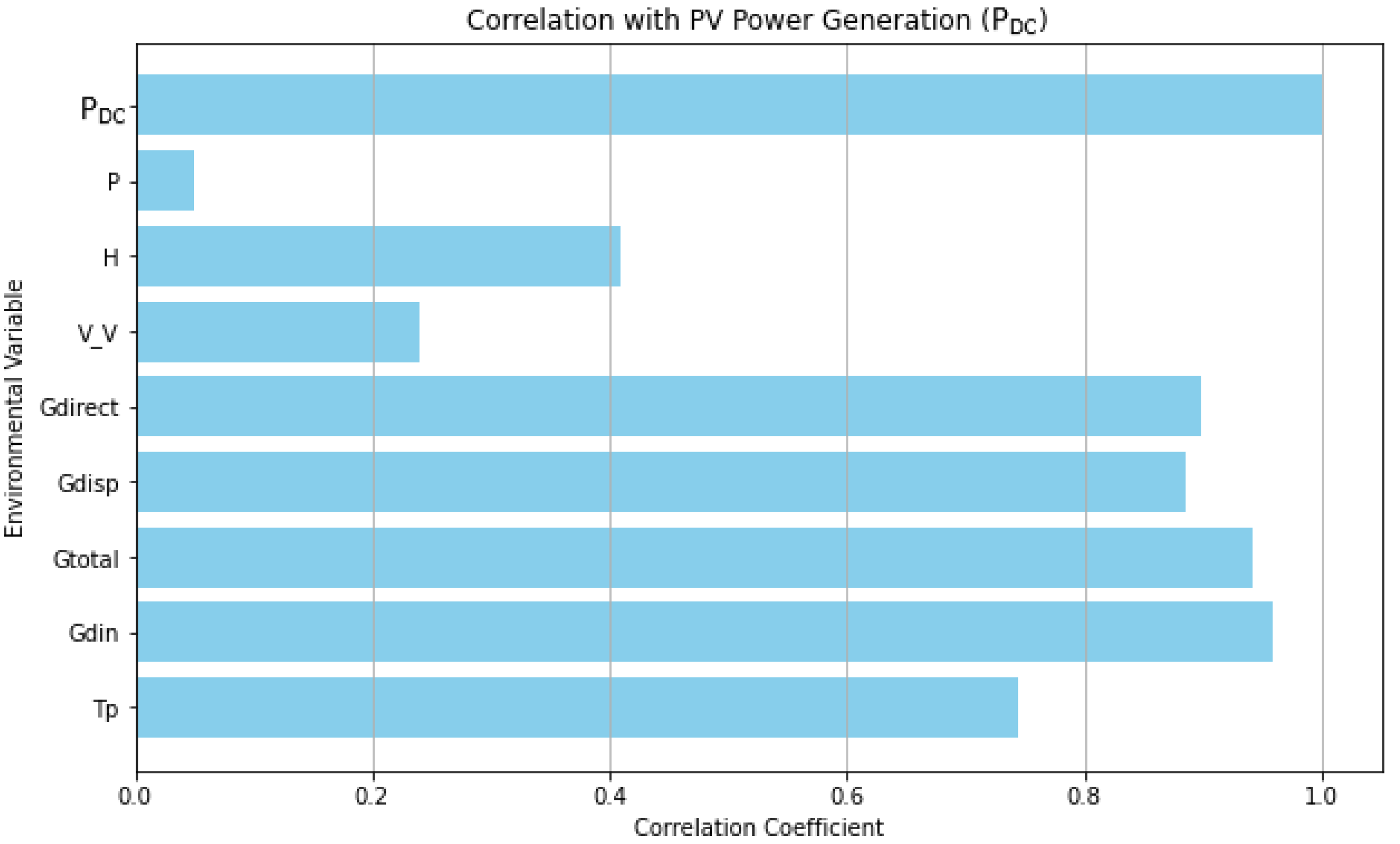
Figure 3.
Distribution of PDC Before and After Removing Outliers.
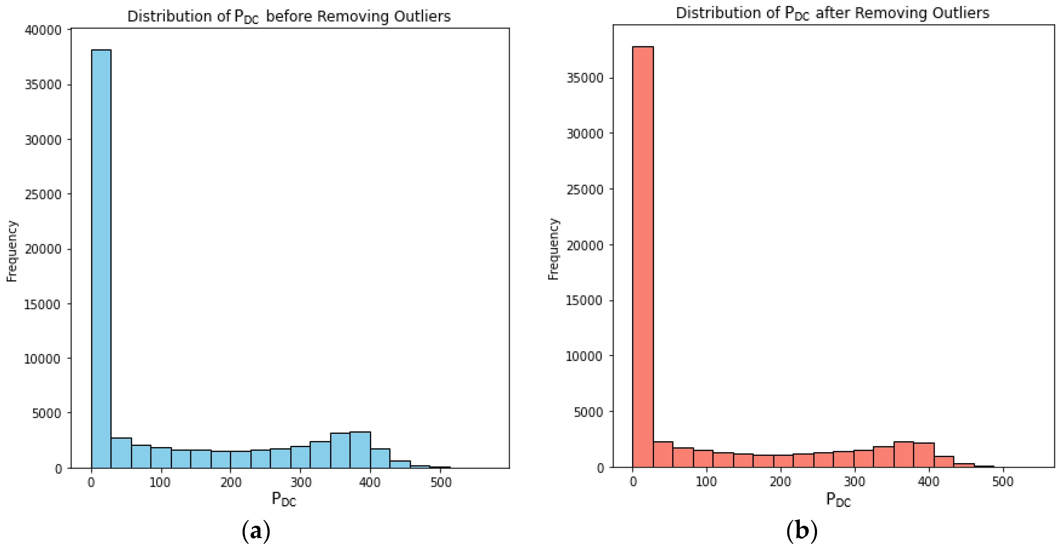
Figure 4.
The methodology framework.
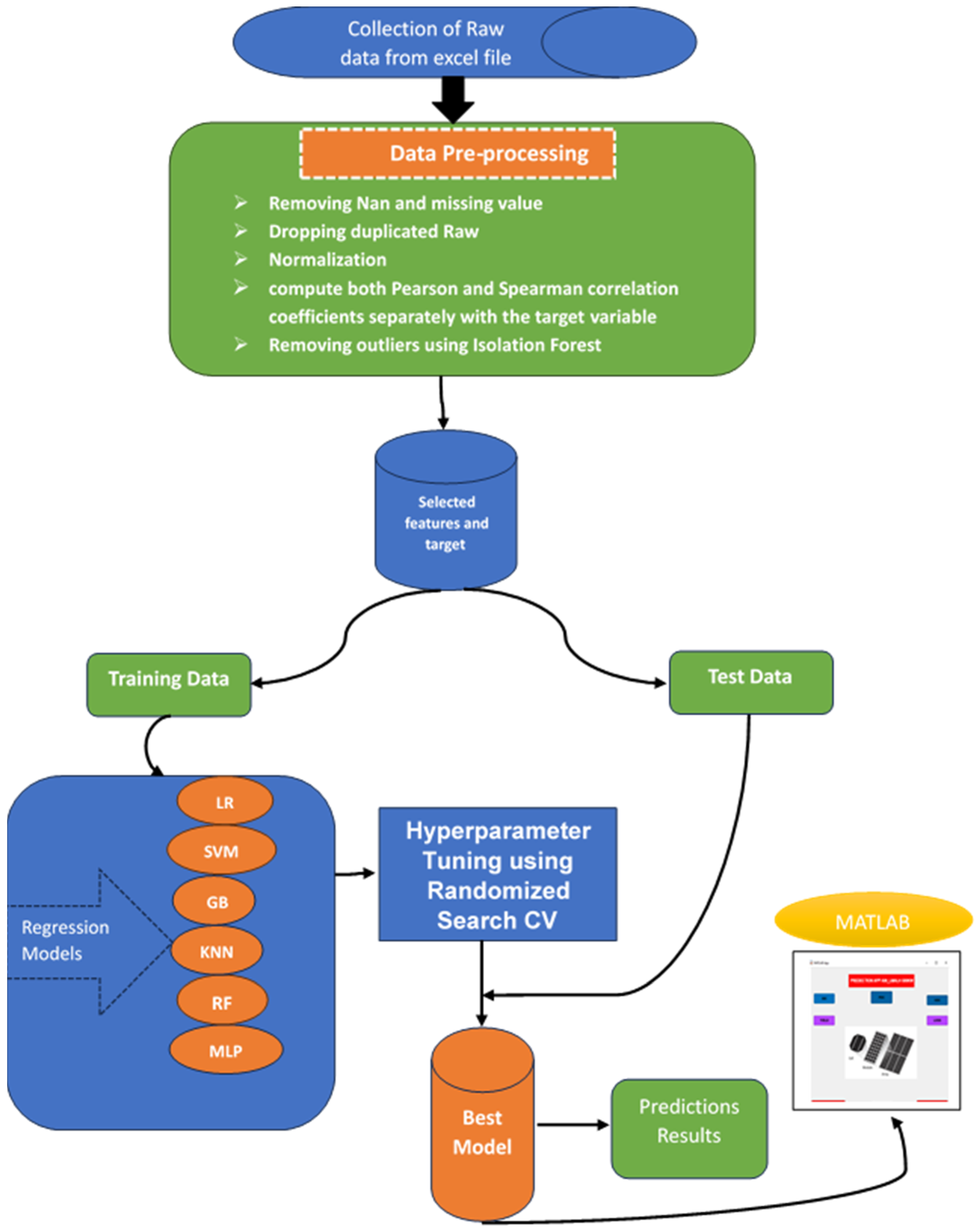
Figure 5.
Process of the used cross-validation technique with 5-fold cross-validation.
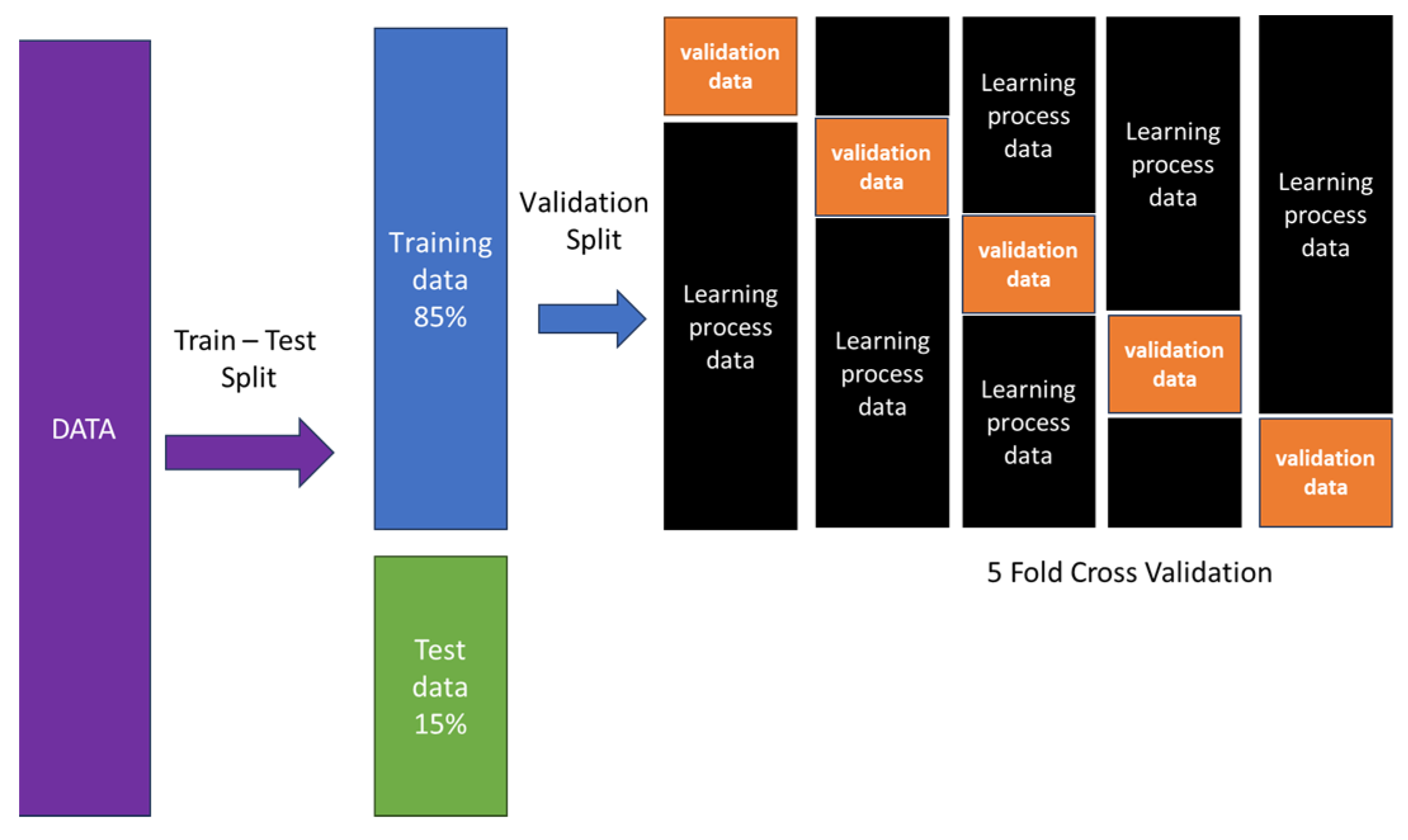
Figure 6.
Main page of the MATLAB App.
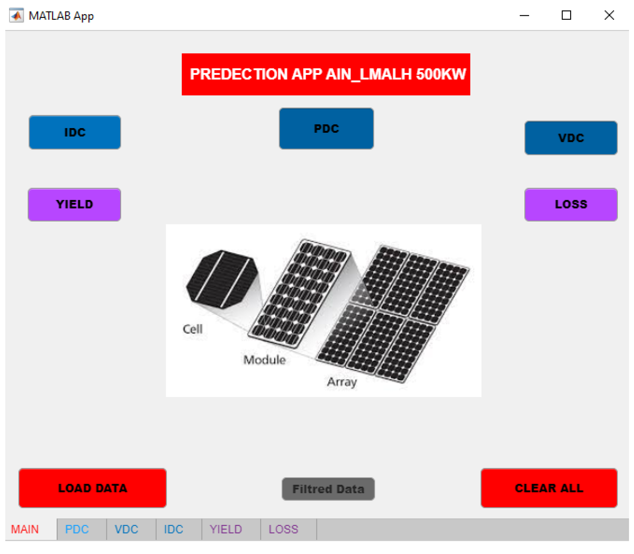
Figure 7.
Performance Ratio (a) and Loss Tab (b) of the designed MATLAB App.
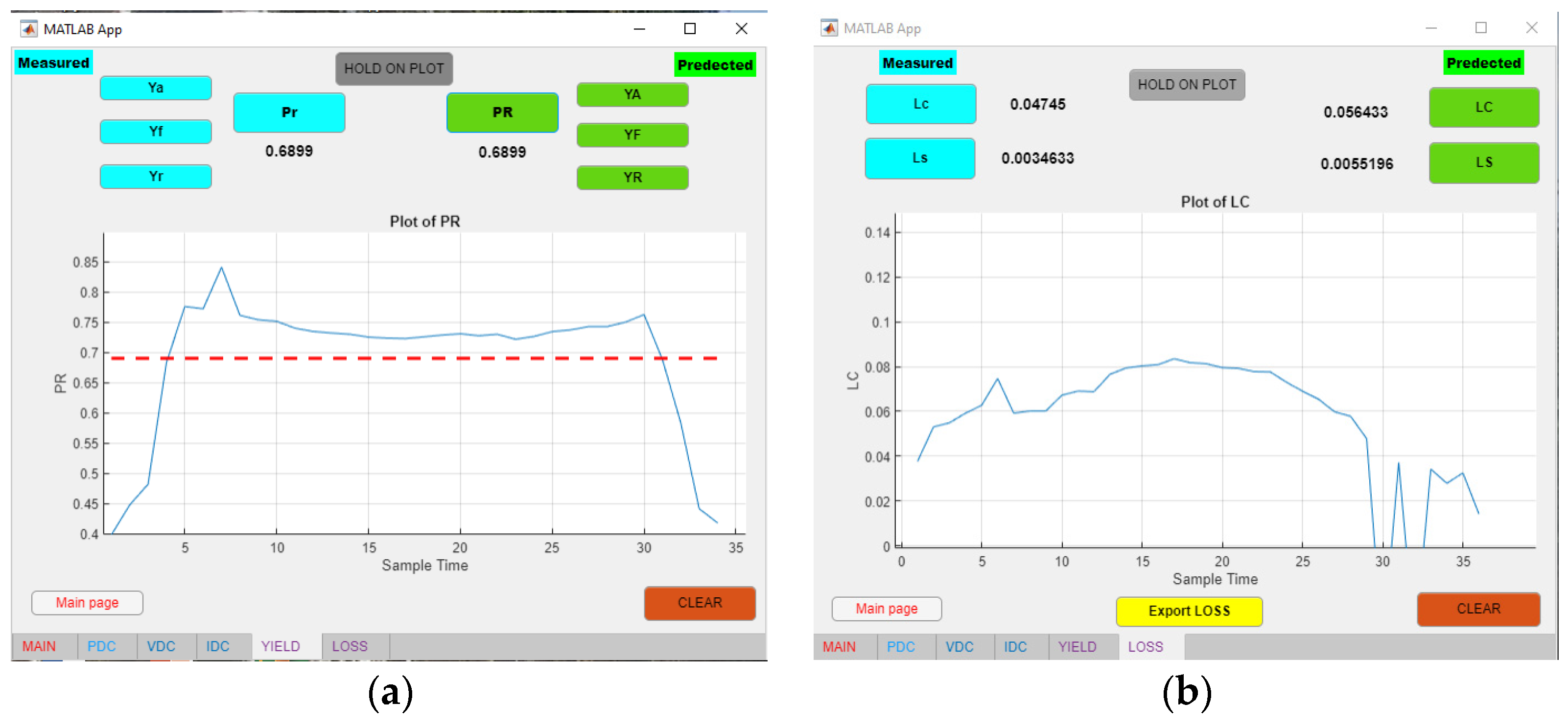
Figure 8.
Random Forest predictions across the test datasets for PDC.
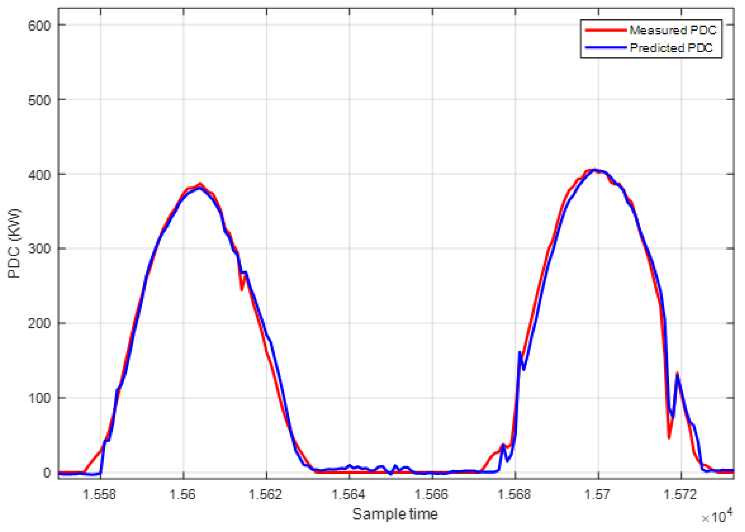
Figure 9.
Actual and predicted plots using RF for PDC.
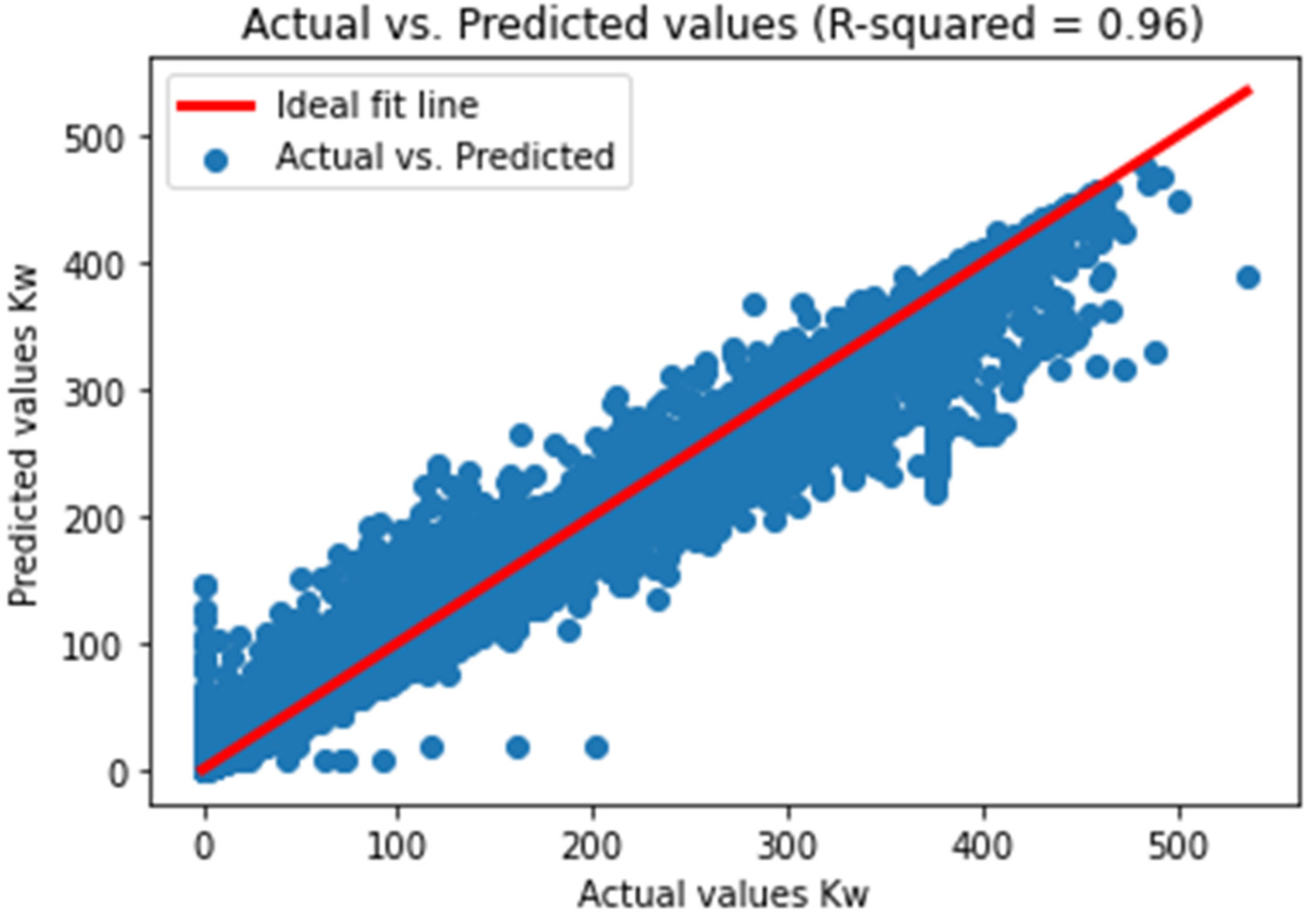
Figure 10.
Error metrics of PDC outputs for the different machine learning algorithms used: RMSE (a), R2 (b), MAE (c) and NRMSE (d).
Figure 10.
Error metrics of PDC outputs for the different machine learning algorithms used: RMSE (a), R2 (b), MAE (c) and NRMSE (d).
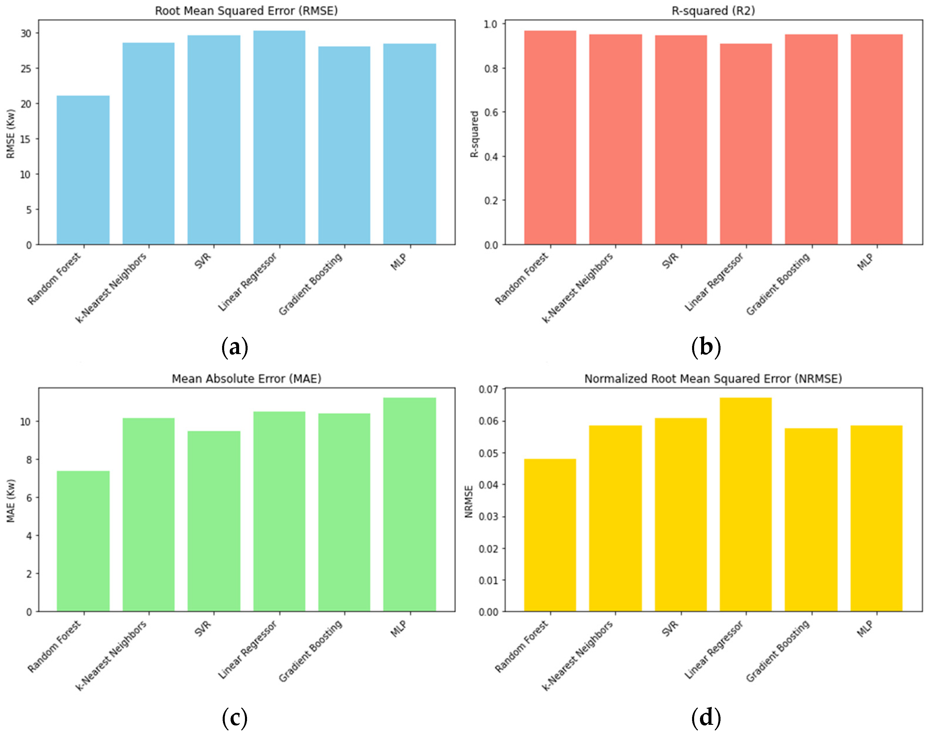
Figure 11.
Random Forest predictions across the test datasets for IDC.
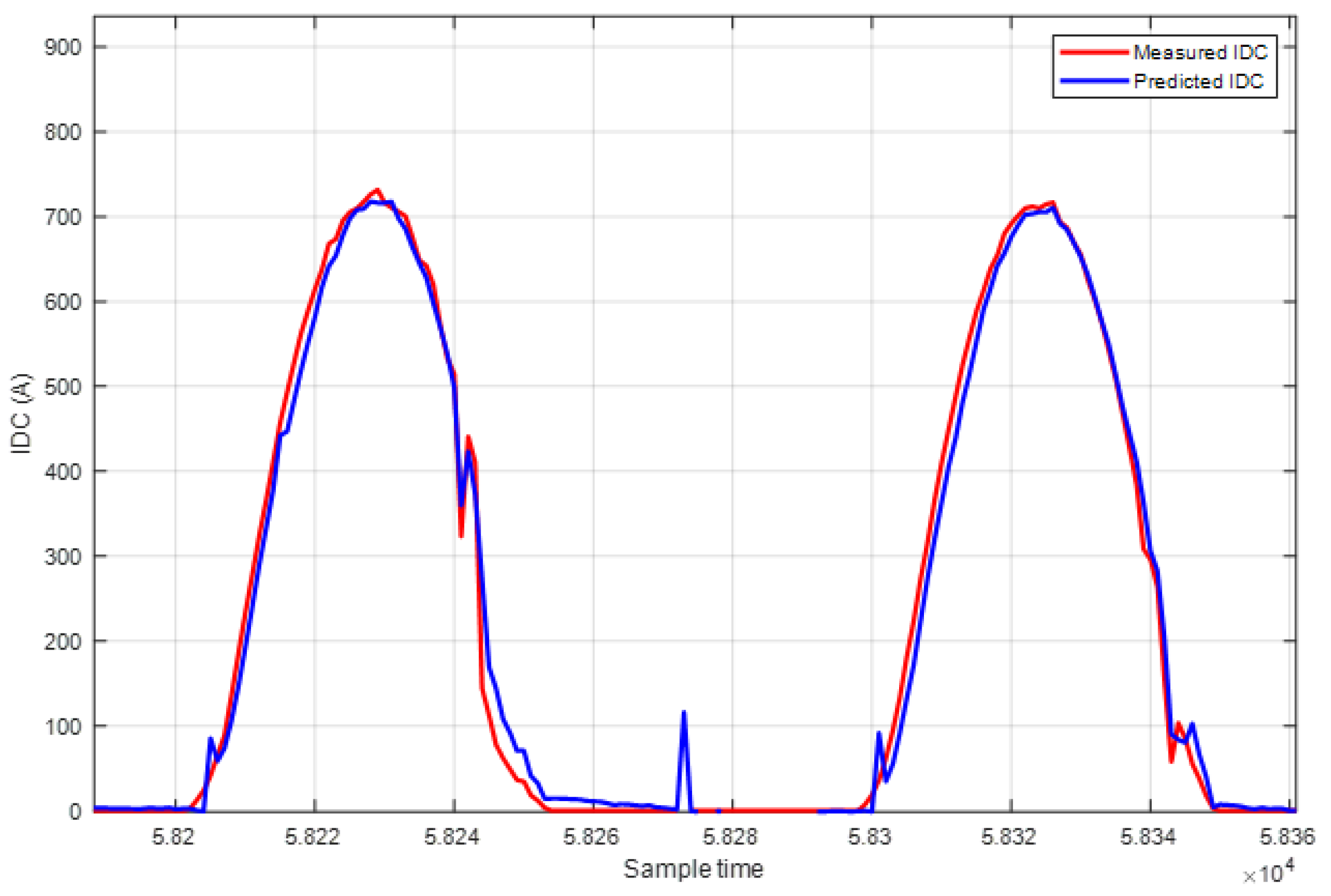
Figure 12.
Random Forest predictions across the test datasets for VDC.
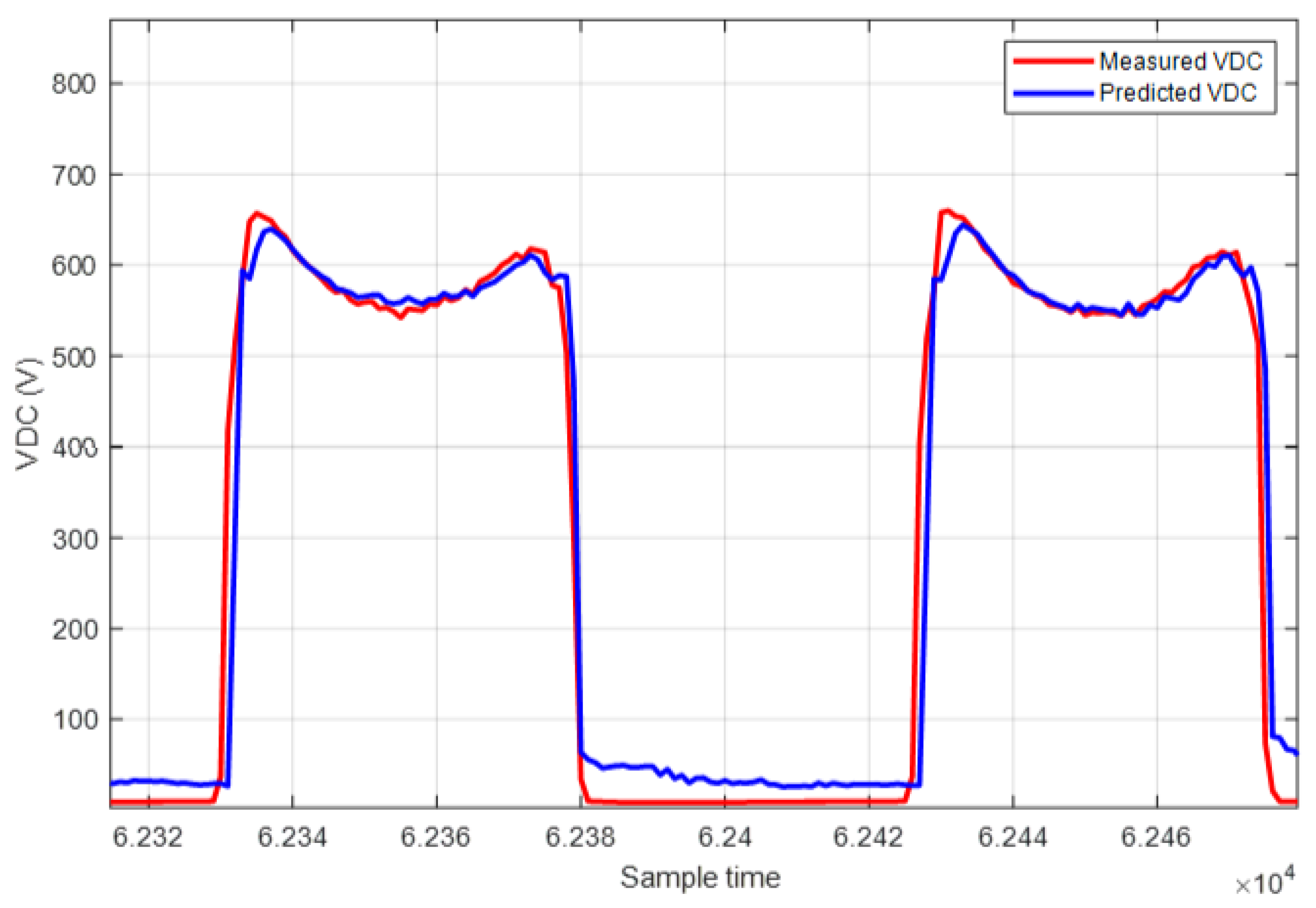
Figure 13.
Actual and predicted plots using RF for VDC.
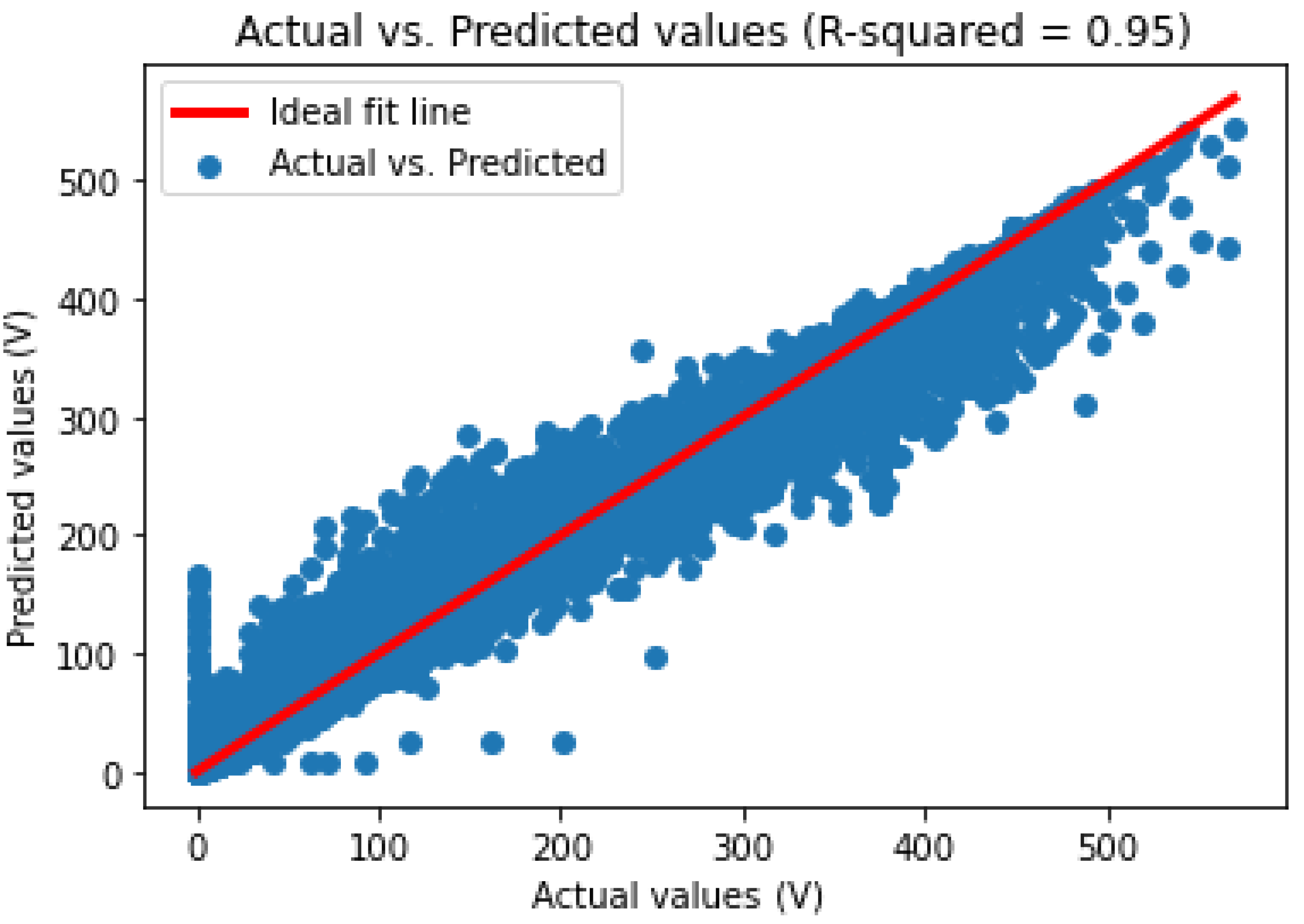
Figure 14.
Actual and predicted plots using RF for IDC.
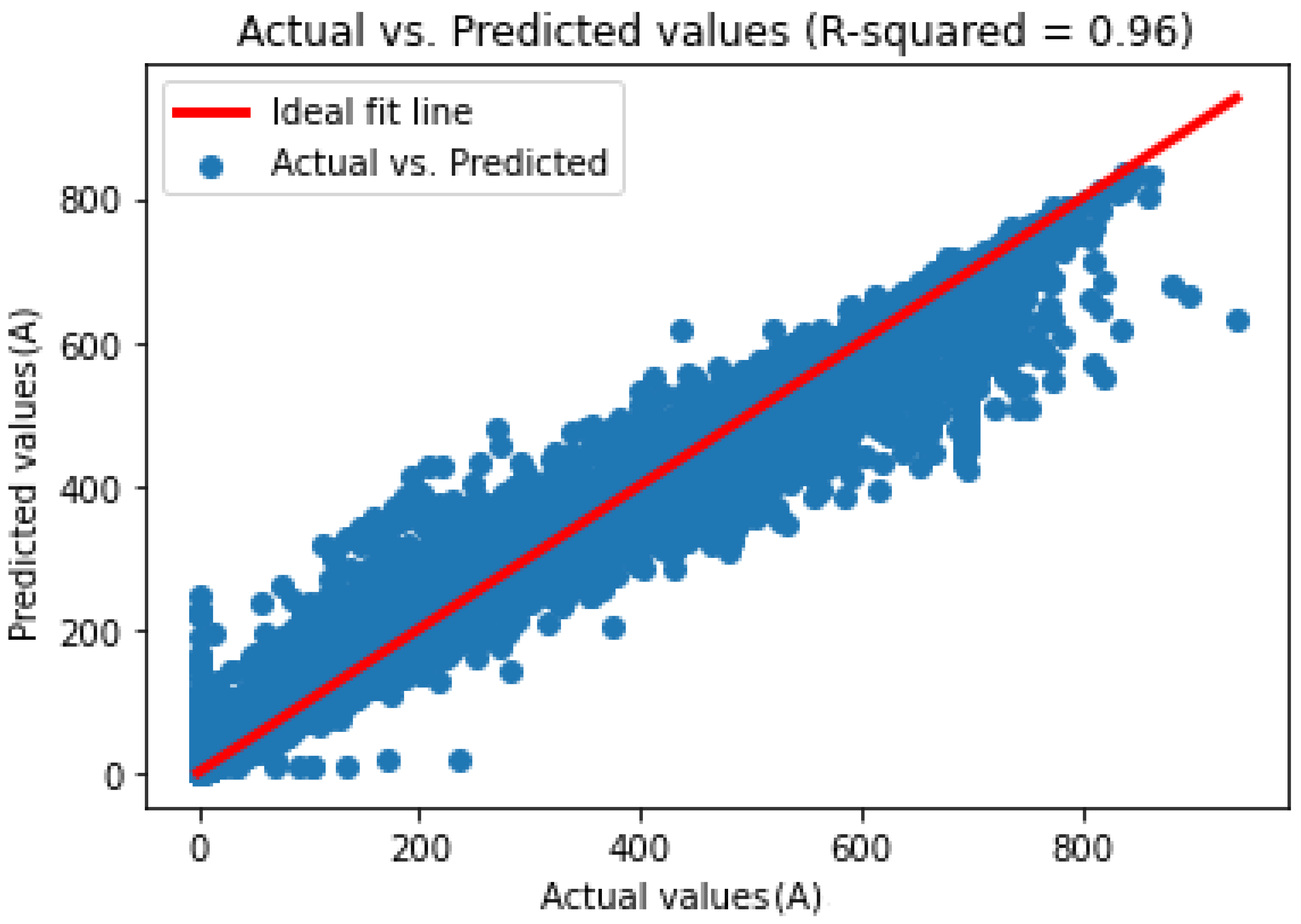
Figure 15.
PDC prediction results obtained from the MATLAB app for Clair day.
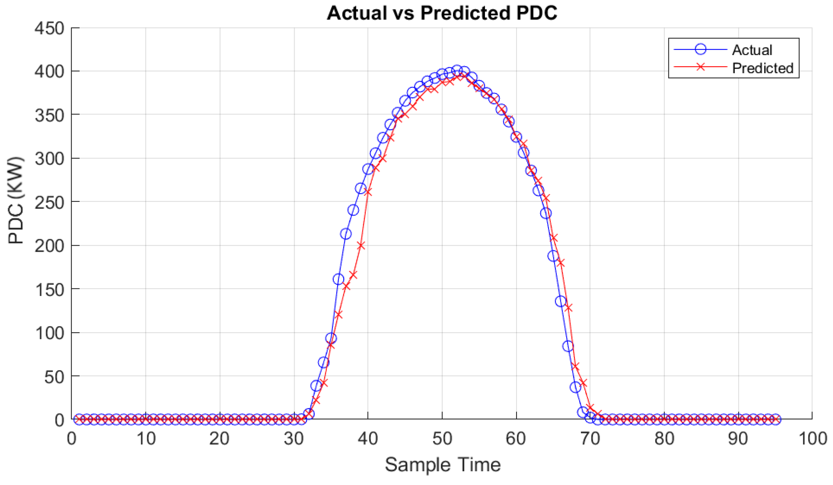
Figure 16.
IDC prediction results obtained from the MATLAB app for Clair day.
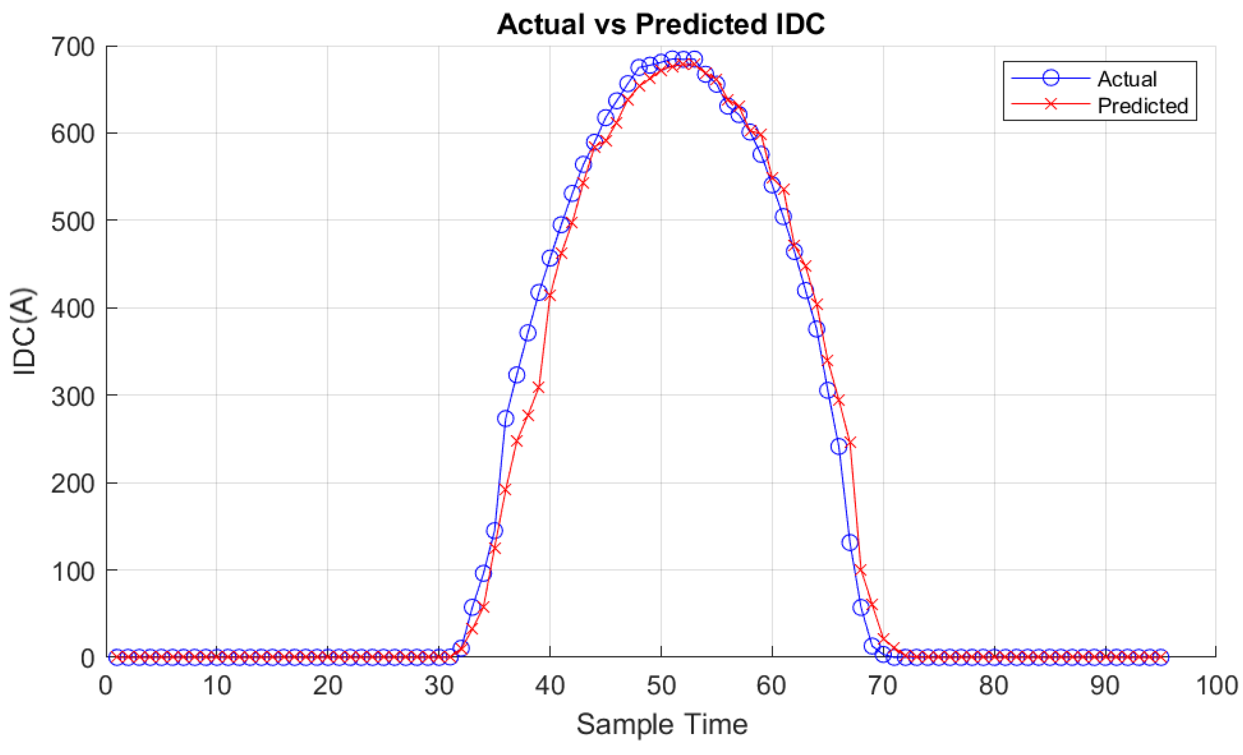
Figure 17.
VDC prediction results obtained from the MATLAB app for Clair day.
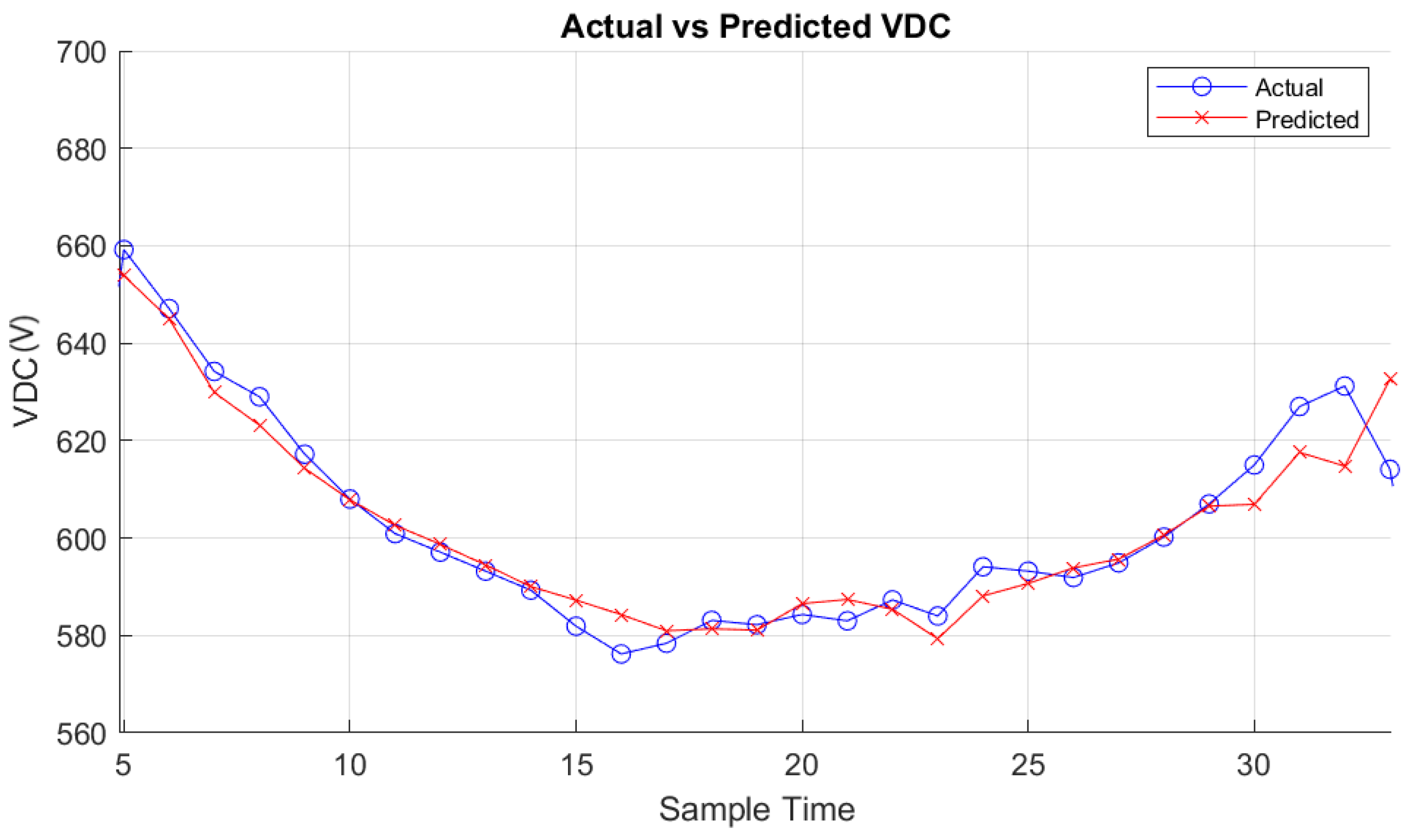
Figure 18.
PDC prediction results obtained from the MATLAB app for cloudy day.
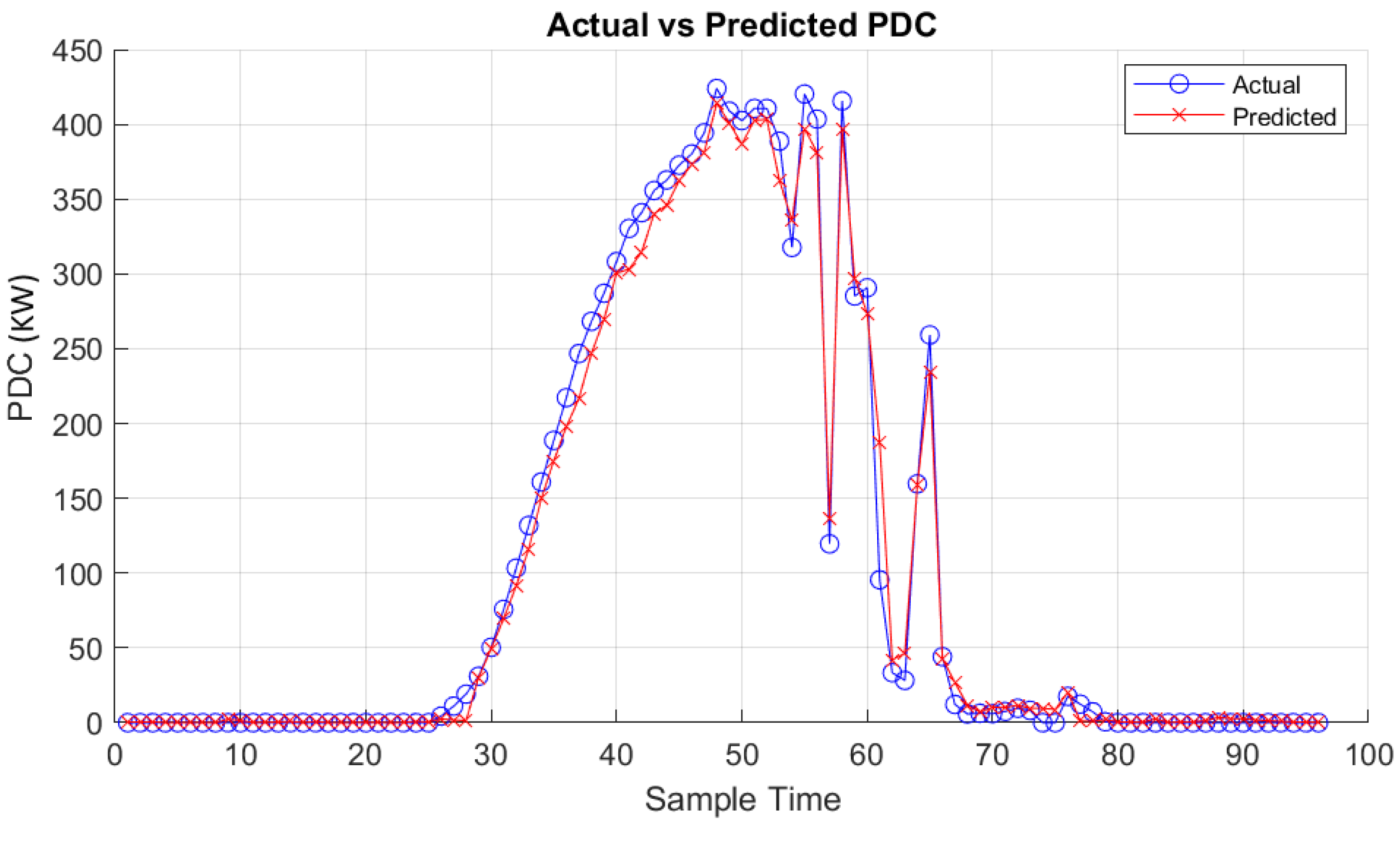
Figure 19.
IDC prediction results obtained from the MATLAB app for cloudy day.
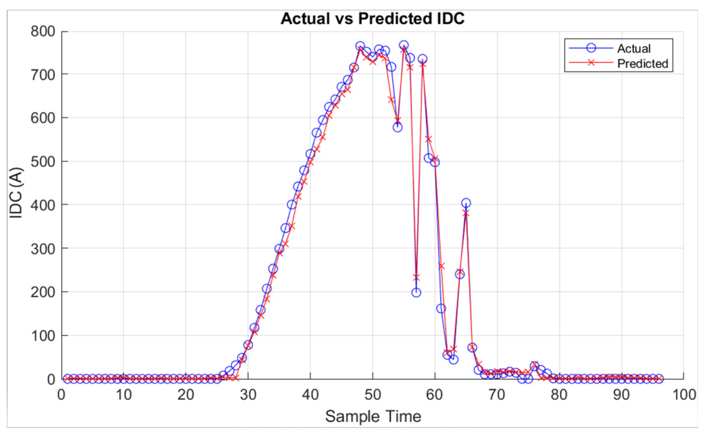
Figure 20.
VDC prediction results obtained from the MATLAB app for cloudy day.
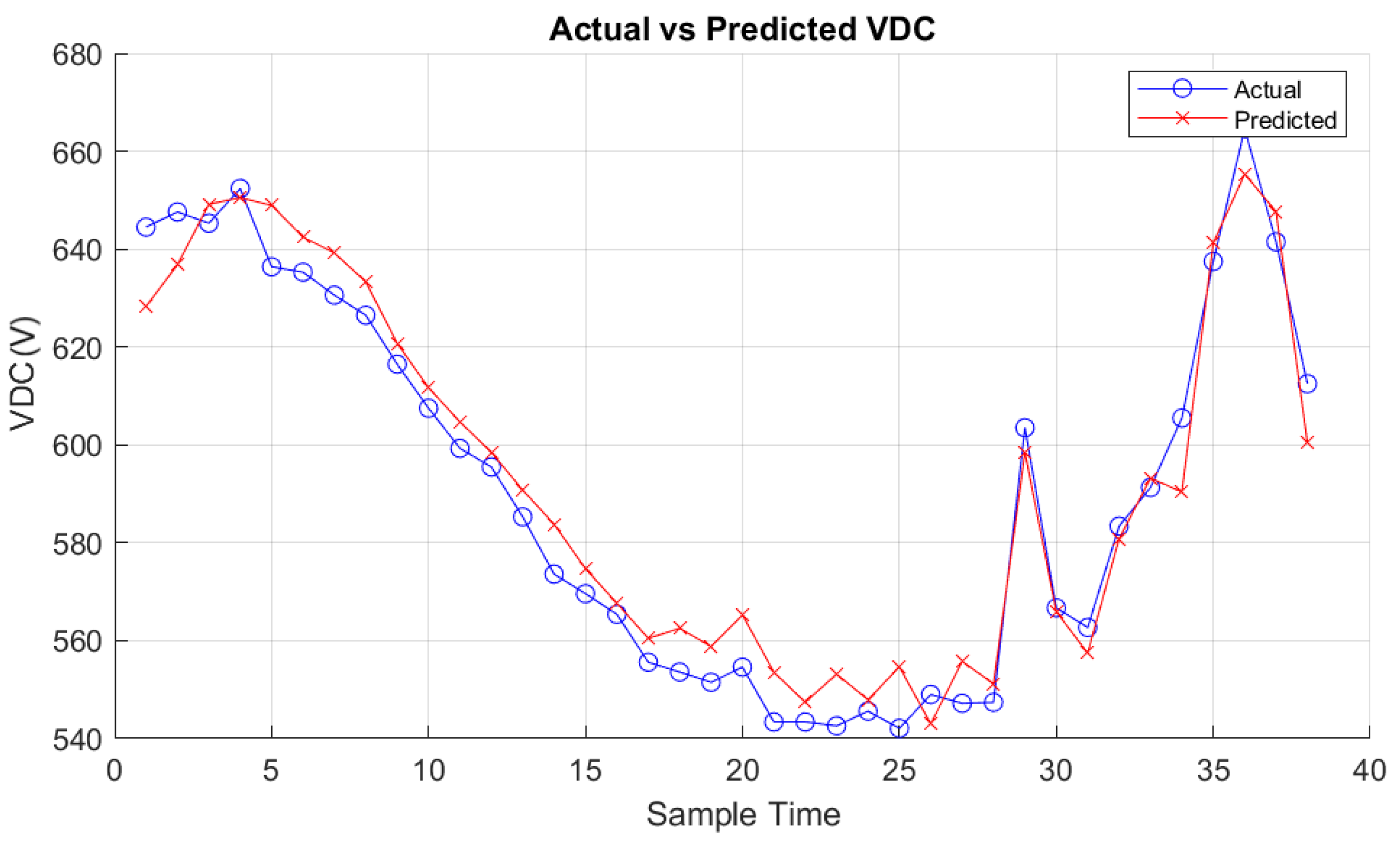

Table 1.
Ain El-Melh PV power plant design parameters (20MWp).
| Parameter | Characteristics |
|---|---|
| Type of module Efficiency of PV module Tilt and Orientation Type of installation PV rows distance Inverter nominal power Characteristics of transformers |
Poly-crystalline silicon 15% 33° South Fixed structure 5 meters 500 KW 1250 kVA, 47–52 Hz, 315 V/31.5 kV |
Table 2.
PV plant monitored data.
| Feature | Description | Maximum | Minimum | Average |
|---|---|---|---|---|
| Tp Gdin Gtotal Gdisp Gdirect V_V H P VDC IDC PDC |
Module temperature (°C) Inclined irradiance (W/m2) Total Irradiance (W/m2) Dispersion (W/m2) Direct Irradiance (W/m2) Wind speed (m/s) Humidity (%) Pressure (Pa) Voltage (V) Current (A) PV power (kW) |
74.800 1651.200 1395.600 686.400 1365.600 22.200 71.600 927.000 780.400 985.400 569.441 |
-2.5 0.0 0.0 0.0 0.0 0.0 0.0 0.0 0.0 0.0 0.0 |
27.987833 310.162255 239.705539 76.567325 232.813488 3.760438 36.119596 912.473873 329.776418 183.593662 108.289535 |
Table 3.
PV modules characteristics (Yingli Solar YL2545-29b).
| PV Module | Specifications |
|---|---|
| STC power rating | 250 Wp ±5% |
| Number of cells | 60 |
| Vmp | 29.8 V |
| Isc | 8.92 A |
| Imp | 8.39 A |
| Voc | 37.6 V |
| Power temperature coefficient | -0.45%/K |
| NOCT (°C) | 46±2 |
Table 4.
Comparative Analysis of Machine Learning Algorithms for Predicting PV Power Outputs.
| Model | RMSE(kW) | NRMSE (%) | MAE(kW) | R2 |
|---|---|---|---|---|
| Random Forest | 21.02 | 0.048 | 7.40 | 0.968 |
| SVR | 29.63 | 0.0648 | 9.51 | 0.9162 |
| MLP | 28.24 | 0.0626 | 9.47 | 0.9509 |
| Gradient Boosting | 27.26 | 0.0575 | 8.60 | 0.9524 |
| k-Nearest Neighbors | 28.54 | 0.0585 | 8.49 | 0.9506 |
| Linear Regressor | 30.26 | 0.0670 | 10.51 | 0.9104 |
Table 5.
Optimization Results and Performance Evaluation of Machine Learning Models for Power Distribution Predictions.
Table 5.
Optimization Results and Performance Evaluation of Machine Learning Models for Power Distribution Predictions.
| Dataset | Parameter | Value |
|---|---|---|
| PDC | Best Parameters | {‘max_depth’: 20, ‘min_samples_leaf’: 2, ‘min_samples_split’: 2, ‘n_estimators’: 200} |
| Best RMSE | 21.02kW | |
| NRMSE | 0.048% | |
| MAE | 7.40kW | |
| R-squared (R2) | 0.968 | |
| IDC | Best Parameters | {‘max_depth’: 20, ‘min_samples_leaf’: 2, ‘min_samples_split’: 2, ‘n_estimators’: 200} |
| Best RMSE | 24.499kW | |
| NRMSE | 0.0476% | |
| MAE | 8.089 kW | |
| R-squared (R2) | 0.957 | |
| VDC | Best Parameters | {‘max_depth’: 30, ‘min_samples_leaf’: 2, ‘min_samples_split’: 2, ‘n_estimators’: 150} |
| Best RMSE | 11.691 kW | |
| NRMSE | 0.060% | |
| MAE | 7.424 kW | |
| R-squared (R2) | 0.953 |
Disclaimer/Publisher’s Note: The statements, opinions and data contained in all publications are solely those of the individual author(s) and contributor(s) and not of MDPI and/or the editor(s). MDPI and/or the editor(s) disclaim responsibility for any injury to people or property resulting from any ideas, methods, instructions or products referred to in the content. |
© 2024 by the authors. Licensee MDPI, Basel, Switzerland. This article is an open access article distributed under the terms and conditions of the Creative Commons Attribution (CC BY) license (http://creativecommons.org/licenses/by/4.0/).
Copyright: This open access article is published under a Creative Commons CC BY 4.0 license, which permit the free download, distribution, and reuse, provided that the author and preprint are cited in any reuse.


