Submitted:
27 May 2024
Posted:
29 May 2024
You are already at the latest version
Abstract
The stability properties of the Hill equation are discussed, and especially those of the Mathieu equation that characterize ion motion in electrodynamic traps. The solutions of the Mathieu equation for a trapped ion are characterized by using the Floquet theory and Hill's Method solution, which yields an infinite system of linear and homogeneous equations whose coefficients are recursively determined. Stability is discussed for parameters $a$ and $q$ that are real. Characteristic curves are introduced naturally by the Sturm-Liouville problem for the well known even and odd Mathieu equations $ce_m(z,q)$ and $se_m(z,q)$. We illustrate the stability diagram for a combined (Paul and Penning) trap and represent the frontiers of the stability domains for axial and radial motion. In case of a Paul trap the stable solution corresponds to a superposition of harmonic motions. The problem of evaluating the maximum amplitudes of stable oscillations for the ideal conditions (taken into consideration) is also approached. Anharmonic corrections are discussed within the frame of the perturbation theory, while the frontiers of the modified stability domains are determined as a function of the chosen perturbation parameter. The results apply to 2D and 3D ion traps used for different applications in quantum engineering, among which optical clocks, quantum logic and quantum metrology, but not restricted only to these.
Keywords:
Mathieu-Hill equation
; Floquet theory
; Sturm-Liouville problem
; perturbation method
; Paul trap
; stability diagram
MSC: 37.10.Ty
1. Introduction
Linear differential equations (LDEs) with variable (periodic) coefficients are ubiquitous in both physics and engineering, but their solutions are generally identified by means of numerical simulations. In an effort to identify a solution for such system, it is essential to infer the so called Floquet or characteristic exponents that define a fundamental matrix associated to the system [1]. One of the most prevalent approaches used in case of LDEs with periodic coefficients is based on truncated Fourier series [2], whose coefficients are derived by means of the Harmonic Balance (HB) approximate method [3,4] that is employed to investigate non-linear oscillating systems described by ordinary non-linear differential equations (NLDEs) [5].
Mathieu functions of period or , also known as elliptic cylinder functions, were introduced in 1868 by Mathieu [6] together with the so-called modified Mathieu functions [7], in order to characterize the vibrations of an elastic membrane placed in a fixed elliptical hoop [8,9]. As the Mathieu equation does not possess closed-form analytic solution, its applications are affected with analytical [10] and numerical approximation schemes [11], along with nonlinear analysis of the associated stability charts [12,13]. Therefore, analytical solutions of Mathieu (Hill) or Duffing equations are generally investigated by means of various perturbation techniques [14,15,16], while other approaches also use non-perturbative techniques to characterize the parametric damping nonlinear Mathieu–Duffing oscillator [17].
During the last 150 years, Mathieu-type linear or nonlinear parametric differential equations have been the subject of large scientific interest, because of their frequent use in applied mathematics [18,19], quantum physics [20,21], quantum optics [22], engineering [12], analytical chemistry, mechanics [13,14], as well as in general relativity [23] and astrophysics [24]. For instance, the Mathieu-Hill equation is employed to characterize periodic orbits in a classical model of the magnetic hydrogen atom in Ref. [25]. An infinite Hill determinant may be computed, which enables one to infer the discriminant of the relevant Whittaker-Hill equation [26] that is used to characterize the stability of the H atom periodic orbits. Such method is less elaborate in comparison with the numerical integrations of the associated orbits.
Analytic periodic approximations for differential equations of Hill type are investigated in [3], where two different methods are employed in the straightforward case of a Mathieu equation. The first method is triggered by the HB method [4,27], with an aim to identify analytic approximations for the critical values and focus on periodic solutions of the Mathieu equation. It is demonstrated that kind of solutions are valid for any values of the parameter q. The second method exploits truncations of Fourier series [2].
1.1. Applications of Mathieu (Hill) Equation in Case of Electrodynamic Ion Traps. Nonlinear (Anharmonic) Traps. Kicked Mathieu-Duffing (Parametric) Oscillator
Scientists have always focused on developing new experimental techniques intended for confining single particles (neutral or electrically charged atoms and molecules, photons, electrons, antimatter, etc.) in a sharply defined region in space, under conditions of minimal perturbations (by creating an almost interaction free environment) [28,29,30,31,32]. This pursuit led to the development of radically new methods aimed at confining atomic and subatomic particles, which resulted in the maturation of optical tweezers, ion trap or magneto-optical (MOT) trap based techniques (including optical lattices) [20,33,34,35]. Prof. W. Paul had the idea of using a rotating or vibrating saddle–like electrostatic potential to confine ions or electrically charged particles [28,36] within a well defined area, under conditions of dynamical equilibrium [37,38]. Ion dynamics in a Paul (or RF) trap is characterized by a Mathieu-Hill type equation [20,39]. The Paul trap apparatus [in case of both 2D linear ion traps (LIT) and 3D versions] has been developed and refined for high finesse quantum engineering experiments, high precision spectroscopy [40,41], along with classical mass spectrometry (MS) [42,43,44,45,46,47] or chemical analysis [48], including the detection of aerosols and chemical warfare [49,50,51,52,53,54,55,56,57]. Besides, ion traps also enable exceptional control in preparing and manipulating atomic quantum states [58,59,60,61,62,63], which is why their wide area of applications also includes quantum logic [64,65,66,67,68], quantum sensing [69,70,71,72], quantum metrology [73,74] and even time fractals [75] or time crystals [76]. To these one adds high accuracy optical frequency standards [77,78,79,80], which are amongst the most sensitive quantum sensors [81,82] used to perform searches for physics beyond the Standard Model (BSM) [83,84,85] or to disseminate atomic time scales and redefine the SI unit of time, the second [86,87,88,89,90].
An electrodynamic trap is highly susceptible to geometric imperfections and electrode misalignment [44,91,92], that lead to the occurrence of local minima in the trapping potential and nonlinear resonances in the ion dynamics [47,93,94,95,96]. In case of 2D traps, motional coupling between axial and radial directions is reported [97,98]. Deviations of the trap potential from an ideal quadrupole lead to parasitic effects [99] and impose limitations on the number of ions that can be confined, and implicitly on the signal to noise ratio (SNR) [70,100,101]. The effects produced by the presence of higher order anharmonic terms [65] of the trapping potential (for linear strings of trapped ions) is investigated in [102], where two distinct effects are emphasized: a) an alteration of the oscillation frequencies and amplitudes of the ions’ normal modes of vibration in case of many-ion crystals, because each ion experiences a different curvature in the trap potential, along with b) significant amplitude-dependent shifts of the normal-mode frequencies, triggered by increased anharmonicity or higher excitation amplitude. As the ratio between the anharmonic and harmonic terms typically increases when the ion-electrode distance is reduced, it is demonstrated that anharmonic effects become more critical by lessening the ion trap scale. This requires special care, particularly in quantum computing with trapped ions [70,103] or in case of single ion [104,105,106] and multi-ion optical clocks [79,107,108,109]. On the other hand, it was demonstrated that an increased dodecapole potential generated in an asymmetric linear ion trap (LIT) [97] opens new pathways for exciting applications in mass spectrometry or Coulomb crystals. Such a setup also enables dark ion (inappropriate confined species) elimination from a trapped ion-chain consisting of physical qubits [47], or performing searches for time and parity violations that could constrain sources of new physics BSM [83,110,111].
Ref. [112] introduces a flow equation to approximate the solution of a weakly nonlinear Mathieu equation (NME), employed to characterize ion dynamics in the neighbourhood of the stability boundary of ideal traps. The HB method [4] is employed in [113] to explore the coupling effects of hexapole and octopole fields on ion dynamics in a quadrupole ion trap (QIT). Ion motion characteristics, e.g. motion center displacement, secular frequency shift, nonlinear resonance curve and buffer gas damping effects have been investigated. It turns out that hexapole fields have larger impact on ion motion center displacement, while octopole fields are mainly responsible for the ion secular frequency shift. In addition, the nonlinear features induced by hexapole and octopole fields may enhance or cancel each other. Ion dynamics in nonlinear Paul traps is investigated in [114] using the theoretical HB method, which allows one to derive the analytical ion trajectory and ion motion frequency in the superimposed octopole field by solving the NME [99]. The HB method is then validated by means of the numerical fourth-order Runge-Kutta (4th RK) method. The incremental HB method alongside with the path-following technique is applied in Ref. [115], where the Mathieu-Duffing nonlinear oscillator model (a Mathieu equation with cubic nonlinear term [4,116]) is employed to explore the steady-state response of a nonlinear piezoelectric energy harvester which undergoes external and parametric excitation. Ref. [115] also establishes that for some specific combination of the system parameters, vibration amplitudes and harvested power can be amplified up to three or five times in comparison to the classical broadband nonlinear energy harvester based on the forced (kicked) Duffing oscillator (DO) [15,116,117]. A method to generate stability plots for the Mathieu equation in case of a toroidal ion trap mass analyser is presented in [118].
The response of a DO to a harmonic excitation in the presence of (viscous) damping is known to exhibit, among other features, hysteretic and chaotic behaviors [1,13,98,116,119]. It is demonstrated that in particular cases the damping force may induce instability in the ion dynamics [120,121]. For instance, Ref. [122] explores the role of field inhomogeneities in altering the stability boundaries in nonlinear Paul traps, taking into account higher order terms in the equation of motion. The Poincaré-Lighthill-Kuo (PLK) method is employed in [123] to derive an analytical expression on the stability boundary and characterize the ion trajectory within a nonlinear Paul trap. The paper shows that a multipole superposition model (which essentially involves the octopole component) explains quite well how the field inhomogeneities shift the stable trapping region.
Particle dynamics in a nonlinear quadrupole Paul trap with octopole anharmonicity (which is a well-known dissipative system [38,124]), is described by a NME [4,125] which includes all perturbing contributions such as: damping, multipole terms of the potential and a harmonic excitation force (periodic kicking). To complicate the picture even more, the ion also undergoes interaction with a laser field [126], in presence of contributions from the hexapole and octopole fields that superpose over the harmonic trap potential. Hence, it was demonstrated that a damped parametric oscillator (PO) levitated in a Paul trap exhibits fractal properties and complex chaotic orbits, along with the emergence of strange attractors (which are often called fractal sets) [126,127]. Ion motion on the strange attractor exhibits sensible dependence on the initial conditions. Several recent papers also demonstrate that ion dynamics within a Paul trap can be assimilated with the equation that describes a damped driven DO [98,99]. The equation of motion for such system is similar to a perturbed Duffing-type equation [15], which is a generalization of the linear differential equation that describes damped and forced harmonic motion [128,129].
Quantum dynamics of general time-dependent three coupled oscillators based on using the unitary transformation method is explored in Ref. [130], which also applies to particle trapping in ion traps and electromagnetic fields. Ref. [131] explores classical and quantum integrability for a trapped ion Hamiltonian in 3D space, under conditions of a non-quadratic potential with superpositions of the hexapole and octopole terms in the series expansion of the electric potential [132]. The Painlevé analysis is employed to determine new integrable cases. It is also demonstrated that the 3D perturbed Hamiltonian is completely integrable in the sense of Liouville [131]. Late results also show the effective potential of an ion in 3D multipole fields in the mixed-mode is characterized by multiple isolated local minima. In addition, the specific number and spatial positions of the stable quasi-equilibrium points depend on the parameters ratio and the polarity of the electrodes DC voltage component [133]. An iterative method is employed to derive the stability parameters from measured secular frequencies, which is presented in Ref. [104].
1.2. Mass Spectrometry with Ion Traps. Late Developments
As the Mathieu equation describes the associated ion dynamics, the dependence of an electrodynamic (Paul) trap on both the ion mass and charge makes confinement of two ion species quite intricate. This is an outcome of the fact that heavier ion species exhibit a lower specific charge ratio, which results in weaker confinement by the RF trapping field [134]. In contrast, confining electrons in a Paul trap requires drive frequencies around 1 GHz, while confinement of different ion species (Al, Ca, Ba, Sr, Yb) requires oscillating electric quadrupole fields in the range of tens of MHz. Commercial Off-The-Shelf (COTS) Quadrupole Mass Spectrometers (QMS) available on the market use oscillating quadrupole fields that operate at frequencies starting from the MHz range (in case of light ions) down to tens of kHz, when investigating heavy molecules characterized by low ratio. Probability plots illustrate that heavy ions are more probably distributed near the maximum of their oscillation amplitude, while lighter ions position themselves at the center of their oscillation [135].
What is more, it is estimated that COTS MS and modified COTS hardware represent versatile tools that are capable of lessening the costs associated with exploration missions [136]. Hence, evaluation and optimization of COTS systems for space mission requirements is presumed to provide affordable analytical tools that enable a wider science community to bring a contribution in space science missions. An example would be the Mass Spectrometer Observing Lunar Operations (MSOLO) [137] that is intended to help NASA’s Volatiles Investigating Polar Exploration Rover (VIPER) mission science team to investigate the chemical composition of the lunar soil and search for water on the surface of the Moon. Another example is the Development and Advancement of Lunar Instrumentation Program (DALI) implemented by NASA. The DALI program has funded the development of the Environmental Analysis of the Bounded Lunar Exosphere (ENABLE) project. One of the tasks of ENABLE- performed at the Southwest Research Institute (sWRI) - lies in adapting a COTS QMS to operate as a space-qualified prototype instrument that could serve aboard multiple mission platforms to monitor environmental conditions under multiple lunar mission scenarios [138,139].
1.3. Ultraprecise Optical Atomic Clocks Based on Ultracold Ions. Current Directions of Action
Different ion trap geometries and electrode space arrangements are generally used (especially hyperbolic and cylindrical traps), in order to achieve a harmonic (electric) trapping potential around the trap centre. Whilst hyperbolic geometries surround the trap centre almost entirely, cylindrical ones usually exhibit open-endcap designs that allow better axial access to the centre and enhanced interaction between levitated particles and laser beams used for cooling or manipulation [140], which makes them suited for quantum logic, quantum optics and quantum metrology applications. For this reason, classical (hyperbolic) endcap electrode geometries are frequently employed when building single ion optical clocks, as they provide certain benefits such as a saddle shaped trapping potential which is essentially quadrupole, along with an open electrode structure that enables effective fluorescence detection [104,106]. Furthermore, a hyperbolic trap potential exhibits true azimuthal angle independence due to the electrode symmetry [141]. An open endcap trap design also exhibits a smaller quadrupole field component in the series expansion of the trap potential, while higher order terms must be considered when calculating the potential apart from the origin. Consequently, a careful trap design must consider and minimize issues such as potential frequency shifts and systematic errors in the atomic clock operation.
The sensitivity of optical atomic clocks [77,142] as quantum sensors is limited by the Standard Quantum Limit (SQL), imposed by the inherent projection noise of a quantum measurement [143]. Recent developments in atomic physics have enabled the experimental generation of many-body entangled states to boost the performance of quantum sensors beyond the SQL [60,71,144,145]. Furthermore, it is anticipated that the use of compound atomic clocks can enhance the stability of single ion clocks with long clock transition lifetimes to levels comparable to that of optical lattice clocks [80,106]. For ion species with shorter lifetimes, the stability can be improved directly by increasing the number of ions, but this approach requires special care in the selection of the atomic transition and offers the potential for a stability beyond the SQL , which could be a viable method to further improve the stability of optical clocks [109] and provide quantum-limited optical time transfer [87,146] to achieve intercontinental clock comparisons through a common-view node in geostationary orbit (GEO). Several missions such as NASA’s Deep Space Atomic Clock (DSAC) or several European Space Agency (ESA) missions are based on deploying optical clocks in space.
1.4. Structure of the Paper
All the aspects presented above motivate the interest towards further investigations on the Hill (Mathieu) class of equations, in order to identify new methods and techniques to mitigate anharmonic effects in case of custom made Paul traps used in laboratories, including anharmonic terms in the potential energy [147]. As the technology matures and the trap dimensions continuously scale down, studies are focused on exploring the anharmonic terms of the RF trapping potential for different implementations (geometries) of a quadrupole Paul trap [101,102]. Even if ion traps are intensely investigated both theoretically and experimentally, the effect of small perturbations from ideal conditions due to higher order (multipole) terms of the electric potential, trap asymmetry and geometric imperfections [92,98], along with patch potentials or other perturbing effects, is an issue of high interest. The paper brings new contributions towards this direction.
Section 1 is also conceived as a review of the applications of ion traps in quantum technologies, mass spectrometry and searches for physics BSM, where among the References the reader will discover some of the most recent advances in the domain. As traps used in experiments across world laboratories are far from being ideal, parasitic effects alter the dynamics of trapped ions and intense efforts are performed to mitigate and minimize their influence. Section 2 investigates the properties of the Mathieu-Hill equations. Based on the Floquet theorem use Floquet’s theorem and Hill’s Method solution, a recurrence relation is inferred. The Brillouin method is also explained. Section 3 investigates stability properties of the solutions of the Mathieu-Hill equation for a trapped ion. It is shown that the solution can be expressed as a Hill series, which introduced into the Mathieu equation yields a recurrence relationship that helps finding the characteristic (Floquet) exponent by employing Sträng’s technique, which is explicitly detailed in Appendix A.1. The stable solution of motion corresponds to a superposition of harmonic motions. The stability diagram for an electrodynamic (Paul) trap is illustrated as a function of the Mathieu function eigenvalues, along with the stability diagram for a combined (Paul and Penning) trap, where both axial and radial dynamics is considered. Ion trajectories in the phase space are discussed and we infer the transfer matrix along with the maximum amplitude of stable oscillations for trapped ions.
Section 4 approaches an issue of large interest by exploring the competition between the ion micromotion and the multipole anharmonicities of the trap electric potential, with an aim to characterize ion dynamics and eventually discriminate between ordered and irregular (chaotic) motion [126]. We supply the modified frontiers of the stability diagram in case of an electrodynamic trap with nonlinear octopole term of the electric potential by using the perturbation theory, as a function of the perturbation parameter we choose.
2. Mathieu-Hill Equations
The Hill differential equation is similar to Mathieu’s equation, but exhibits a more general nature. It arises in Hill’s method [148,149] to establish the motion of the Lunar Perigee and it represents a generalisation of the Mathieu equation [18,26,150]. The Mathieu-Hill equation is a homogeneous, second-order ordinary differential equation (ODE) with variable (periodic) coefficients [4,13]. It characterizes dynamical systems that exhibit intrinsic periodicity and parametric behaviour, such as modulation of radio carrier waves, transverse vibrations of a tense elastic membrane, stability of periodic motion in a non-linear system, the focus and defocus of beams in particle accelerators [151,152], or it is employed to explore planet dynamics [24]. The Hill equation takes the canonical or standard form of a reduced linear equation of the second order [8,10,19,153]:
where J stands for a continuous and even function, periodic in . The period is usually taken equal to for historical reasons [153]. The differential equation (1) was discussed by Mathieu in 1868 in connexion with the problem of vibrations of an elliptic membrane [6]. It is also assumed that the function can be expressed as a Fourier series [26]
which converges within an infinite band in the plan that includes the real axis. If for , then eq. (1) turns into the Mathieu equation. What is more, eq (1) can also be arranged as:
where represents a continuous and even function of period , while a and q denote adimensional parameters [154]. In the particular case of Mathieu’s general equation or Hill’s equation, a fundamental system of solutions consists of and , as the equation is invariable to the change . Consequently, Floquet demonstrated that the complete solution of Mathieu’s general equation (1) can be expressed as [26,150,153,155,156]:
where is called Floquet or characteristic exponent and it is a definite function of the a and q parameters, is a periodic class function (twice continuously differentiable) [157], while stand for arbitrary constants. Then, based on the Floquet theorem and according to Hill’s method one may assume a series solution
By introducing eq. (5) into eq. (1) one infers a recurrence relation:
where is the set of integer numbers, while . If one tries to eliminate the term in eq. (6), then a nonconvergent infinite determinant [26] would result. To avoid such an outcome, every expression in eq. (6) is divided to its central term . To determine the characteristic exponent, one multiplies the system matrix described by eq. (6) with a diagonal matrix. Then, a matrix results whose diagonal entries are each one equal to unity, assuming that none of the terms vanishes. By denoting the determinant of this matrix as , the equation that determines the Floquet exponent is [26]
What is more, eq. (7) can be further arranged as:
When has been determined, the coefficients can be inferred in terms of and co-factors of . Thus, the solution of the Hill differential equation is complete. In case of a fairly rapid convergence of the determinant , eq. (7) can be used in its algebraic as well as recursive and explicit form, which represents Hill’s original method [9,26]. Evaluation of the determinant and use of eq. (8) represents an alternative method when this determinant converges quite well. A practical method to solve the Hill equation was suggested by Brillouin [153], based on the expression
where and stand for two fundamental solutions. If a periodic fundamental solution exists for the Mathieu equation, then the existence of the other fundamental solution is forbidden and the characteristic exponent of the periodic solution corresponds to the a and q parameters of the characteristic curves that separate the stability domains. In case of the Hill equation, such property is not generally satisfied. Eq. (9) is useful to compare with Whittaker’s theory on the Hill equation [26]. The advantage of applying such method lies in the fact that it works with periodic functions that exhibit a finite number of discontinuities.
For example, Ref. [158] investigates the modes which diagonalize the dynamical problem for linearly coupled Mathieu equations, which leads to the Floquet–Lyapunov transformation where the motion is associated with decoupled linear oscillators. The method is then used to solve the Heisenberg equations of the corresponding quantum-mechanical problem, and to determine the quantum wavefunctions for stable oscillations in the configuration (Hilbert) space. Such transformation and solution can be applied to more generic linear systems with periodic coefficients, such as coupled Hill equations and periodically driven parametric oscillators.
3. Stability of the Solutions of the Mathieu-Hill Equation for a Trapped Ion
The equation of motion for an ion confined within a Paul (electrodynamic) trap exhibits the standard form of the Mathieu equation [18,159,160,161]
with dimensionless, where is the RF of the trapping voltage applied between the electrodes. To investigate the stability of ion trajectories one uses the stability properties of the Mathieu equation solutions. As shown in eqs. (4) and (5), the solution of eq. (10) can be expressed as a Hill series
where the A and B constants are determined from the initial conditions. If , then using eq. (11) one infers a fundamental system of solutions associated to eq. (10) for and (the Floquet theorem [18,26]). The characteristic exponent and the coefficients are functions of the parameters a and q [159].
By introducing the solution supplied by eq. (5) in the Mathieu equation (10), the latter is cast into
which after matching the terms according to the powers of s results into a recurrence relation
One further multiplies with and then divides with the middle term in eq. (13), which leads to an infinite system of linear equations which are homogeneous in the coefficients [155]:
which can be written as
with
The system of equations (15) admits a nontrivial solution if and only if the corresponding infinite determinant vanishes for s noninfinite [26,162]
Due to the symmetry of , . Solving this determinant is not a simple issue, which is why one uses the approach of Whittaker [26]. The method is described in Appendix A, and it was introduced by Sträng [162,163]. The equation
supplies the characteristic exponent , while eqs. (15) enable one to recursively determine the coefficients . The infinite order determinant is absolutely convergent and it represents a meromorphic function [164,165] of , with simple poles for . Hence, eq. (17) is equivalent with [18]
Hereinafter we discuss the stability of the solutions of eq. (10) for . The solution of eq. (11) is stable and respectively unstable, if is bounded, respectively unbounded along the semi-axis. From eq. (19) one infers , which renders the solution of eq. (11) as stable when , so for real non-integer. If , then , while is bounded along the axis. In such case is bounded along the semiaxis only when or . As an outcome, the plan is divided into stability regions with and instability regions characterized by , separated by the curves for which a stable and periodic solution of eq. (10) exists, although the general solution is unbounded. The curves characterized by integer values of are called characteristic curves. They are naturally introduced by means of the Sturm-Liouville (eigenvalue) problem [26,154,166] for the Mathieu functions and [19,161], which are treated as characteristic functions of eq. (10) with the limit conditions
The and functions [7,167] are even and odd respectively, known up to a constant factor, with period when m is even, and with period for m odd [18,26]. The characteristic curves and , correspond to the Mathieu functions with , respectively , with . In addition, the characteristic curves are analytical in q, while being characterized by the subsequent properties [26]
with , and .
The family of curves characterized by coincides with the family made up by the characteristic curves with , and with , which divide the plan into stability regions [ranging from to for , and from to or from to for ], and instability regions located below or ranging from to .
Ref. [168] shows that in case of microparticles levitated within a 2D linear Paul trap (LPT) operating under Standard Temperature and Pressure (STP) Conditions (in air), the Mathieu equations describing the trapping process are homogeneous along the x and y axes, with the well known solutions and stability domains. On the other hand, the z-axis motion is described by an inhomogeneous Mathieu equation. In this case, stability is obtained for (a) ; (b) and (c) and , where is the Floquet exponent, , K stands for the coefficient which describes the drag aerodynamic force and m represents the particle mass. Hence, stability regions for solutions of the inhomogeneous equations of motion in presence of drag forces include both the stability regions of the homogeneous equations along with a part of the instability regions, which extends them considerably.
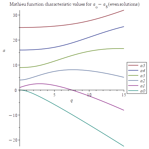
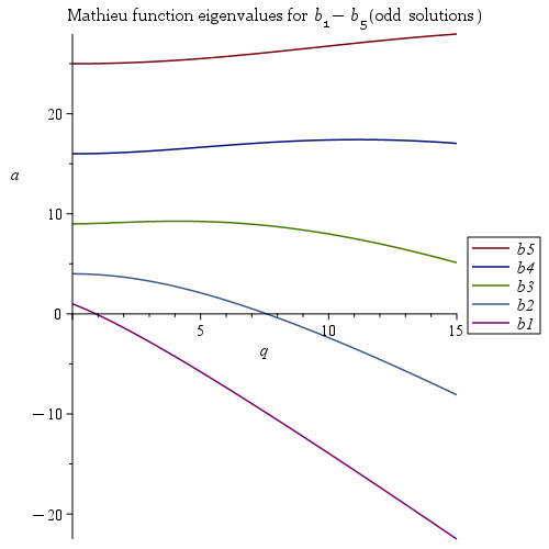
The Mathieu equation (10) exhibits and periodic solutions on continuous stability curves , starting from points . What is more, the periodic solutions and the boundaries between stability and instability regions in the parameter plane can be found by means of the Lindstedt-Poincaré method [16]. A cosine elliptic and a sine elliptic functions are associated to any value of n, where each one of these functions has its own characteristic number and . The Mathieu functions and their eigenvalues (characteristic numbers) in power series of q, for , are expressed as:
The eigenvalue associated with the even solutions of the Mathieu functions, is labelled by , while the one associated with the odd Mathieu function, , is denoted as , as illutrated in Figure 1. The higher rank terms that describe the frontiers of the stability regions are given in Appendix B. To graphically illustrate the stability diagram (associated to the Mathieu equation) that characterizes the dynamics of an ion confined within a combined quadrupole trap (a combination between a Penning and a Paul trap), we have used eqs. (23 - 27) and eqs. (A20 - A28). The result is shown in Figure 1.
The stable solution of the equation of motion (10) (for ) corresponds to a superposition of harmonic motions [20,31,101]
with the frequency spectrum
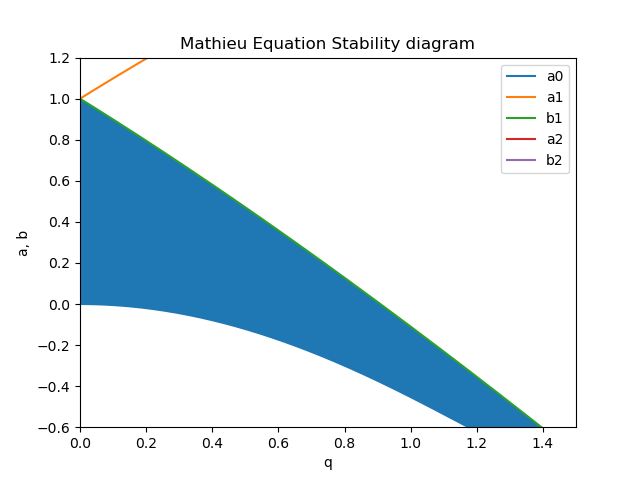
In Figure 3 we have illustrated the stability diagram for a combined (Paul and Penning trap). One notices that represent the frontiers of the stability diagram associated with the canonical Mathieu equation that describes axial motion. We also introduce
Further on, we will consider trap operating points of that lie within the first stability region, with and . By minimizing the parameters a and , the coefficients (with ) rapidly converge to zero, in such a way that higher harmonics are practically insignificant and the fundamental frequency prevails [169]. In such event , where stands for the average of the shift during the interval and . Under such circumstances, the solution of the Mathieu equation can be approxi-
mated as the solution of the equation
By averaging eq. (33) over a period of the RF voltage (which is exactly the case of the pseudopotential approximation, when the electric forces that are time-averaged over an RF period generate a harmonic potential [20,31,170,171]), one derives
The shift in eq. (34) corresponds to the harmonic motion of fundamental frequency , while the correction is determined by the higher harmonics , . The axial frequencies are twice the radial frequencies: and , while the trapped ions describe approximate Lissajoux trajectories when the ratio between the frequencies along the axes is . The initial conditions have no effect whatsoever on the stability of ion trajectories, but they establish their position with respect to the area located between the trap electrodes for every operating point fixed within a stability domain. In this regard, the problem of evaluating the maximum amplitude of stable oscillations under given initial conditions is approached. The maximum admits upper bounds determined by the relative position of the electrodes. For optimum operating parameters it is mandatory to take into account all axes for whom the equation of motion is of Mathieu type.
One considers the stable solution of eq. (28) expressed as
with
where both and are differentiable functions. If (which also implies that the coefficients ), then and are linearly dependent functions. Hence, and form a fundamental system of solutions of the Mathieu eq. (10) and the Wronskian determinant [7] is
Furthermore, the derivative of the Wronskian determinant is
The modulo of the solution of eq. (35) admits the following upper limit
One denotes
Hence, for an initial given phase , eq. (43) represents the equation of an ellipse of area in the plan . For initial conditions given such that the point is located on the ellipse described by eq. (43) or within it, one finds at any moment in time. The ions are not captured at the electrodes if all points w (with ) belong to the projection along the w axis of the region located within the electrodes.
To investigate ion trajectories in the phase space it will suffice to build the family of ellipses described by eq. (43), for ranging between . Indeed
with the transfer matrix expressed as
The maximum amplitude of stable oscillations for trapped ions results from eq. (43)
3.1. the Kicked Damped Parametric Oscillator
One considers the differential equation (DE) which describes a damped, kicked parametric oscillator (PO)
where and h are continuous functions of , while stands for the kicking term, which is usually a periodic. The homogeneous equation
exhibits the fundamental solutions which we denote as and . Then, the general solution of eq. (48) is expressed as
with is the Wronskian determinant. Eq. (49) changes into the normal form
with
In particular, if the J function is periodic and continuous, the normal form described by eq. (51) is a Hill equation. In case when f is a constant function , one derives
It can be noticed that the solution of eq. (48) is stable if , with the Floquet exponent given by eq. (4). If w is stable, then definitely u is also stable. Nevertheless, there exist unstable solutions w for which the corresponding solutions u are stable. The frontiers of the stability domains are supplied by the equation .
4. Anharmonic Corrections for Electrodynamic (Paul) Traps. Perturbation Method Analysis
An issue of large interest lies in exploring the competition between the ion micromotion and the multipole anharmonicities of the trap electric potential, in order to discriminate between stable and unstable (chaotic) dynamics [172,173,174,175]. Ref. [126] reports on the dynamics of an ion confined in a nonlinear Paul trap [61,122,176], assimilated with a time-periodic differential dynamical system. As such systems are characterized by low dissipation, exotic phenomena can be observed such as strange attractors, limit cycles, period doubling bifurcation and fractal basin boundaries [75,127,175]. We investigate the following equation of motion, which describes the axial dynamics for a particle of mass M and electric charge Q, confined within a quadrupole Paul trap, with anharmonicity derived from an octopole (quartic) electric potential [126,177]:
where the adimensional parameters a and q are expressed as
while and stand for the Paul trap radial and axial dimensions. Generally, in case of a typical 3D Paul trap, and . The frequency of the applied a.c. voltage (micromotion) is denoted by , and stand for the static and time-varying trapping voltages, respectively. Analytical modelling of the dimensionless equation (54) is based on employing techniques characteristic to the global bifurcation theory [14,128]. Numerical modelling is used to explore the associated dynamics and discuss chaos in such a nonlinear system [172,173,174,175].
Further on we introduce the perturbation parameter and choose , with the anharmonicity parameter fixed. Then, one can perform a series expansion of the a parameter and z coordinate as a function of the parameter:
4.1. Solutions of the Mathieu Equation
The frontiers of the stability domains in the plan of the control parameters are determined by the periodic solutions of eq. (54) [104,126]. There is a requirement that z is a periodic solution, of period and known parity, Within the limit the z solution is expressed as or , with . One considers the case when , with an anharmonicity parameter. Then, eq. (54) writes as
whose solution can be expressed as . Then, and eq. (57) changes into
We use the expression for derived above and revert to eq. (54)
Then, eq. (61) can be cast into
Therefore, by employing eqs. (56) and (54), after identifying the rank of the parameter, one infers a system of differential equations that recursively determines the parameters and coordinates:Eq. (62) can be expressed as
where or , with . Therefore, the frontiers of the Mathieu stability diagram are either even functions or odd functions that depend on the parameter q, which within the limit approaches , respectively . The k and j indexes are integer, with cu and . By performing a series expansion of these functions depending on q parameter , one derives the first frontiers of the stability diagram [178]
where and is a constant.
Hence, the frontiers of the stability diagrams for the Mathieu equation with anharmonic perturbation are characterized by eqs. (64) - (67). It is evident how the frontiers of the stability diagram are shifted towards negative values along the a axis, in the control parameters plan . Figure 4 and Figure 5 illustrate the stability diagram for the dynamics of an ion in the anharmonic trap we have investigated.
It can be noticed that the first stability region is bounded by the curves a̧nd , while the second stability region is bounded by the curves and , respectively. As opposed to the pseudopotential approximation when the electric RF potential is described by a polynomial of rank 2 in [20,30,31,114,156], consideration of the micromotion leads to stability regions that are qualitatively similar to those of the Mathieu equation for low enough values of c, but generally with frontiers sensibly altered as a function oi the anharmonicity parameter . Hence, explicit analitic calculus which is numerically illustrated, enables one to establish the differences between the stability domains of the nonlinear dynamical system that is periodic in time (described by eq. (Figure 5)) and those of the autonomous dynamical system that is associated by means of the pseudopotential approximation [171].
4.2. the Frontiers of the Stability Diagram for the Mathieu Equation with Nonlinear Term
This section of the paper presents the technique we have developed to derive . The frontiers of the stability diagrams of the Mathieu equation with nonlinear term (anharmonic perturbation) are given by eqs. (64 - 67), which correspond to the following limit solutions for :
The motion of a single charged particle in a nonlinear Paul trap, in presence of the damping force, is investigated theoretically in [120] and the modified stability diagrams in the parameter space are calculated. The results show that the stable regions in the parameter plane are not only enlarged but also shifted. Our results also show that the frontiers of the stability diagrams for the Mathieu equation are shifted towards negative values of the a parameter (within the plan defined by the control parameters ). In disagreement with the pseudopotential approximation for a Paul (RF) trap [114,171], when the electric potential is described by a polynomial of rank 2 in , by taking into account the micromotion (when not in the pseudopotential approximation) stability regions result that are qualitatively similar to those of the Mathieu equation, but with frontiers that are shifted depending on the anharmonicity parameter . Further on we express eq. (63) in case as
and we compute the right term for . Then, the right hand of eq. (69) is cast into
which can be further expressed as (See Appendix C)
One writes
as
Then, one derives
Hence, eq. (74) becomes
Using eq. (75) we infer
Then, eq. (69) becomes
The general solution of the harmonic oscillator (HO) writes as
We choose an even solution, such as . Then, one tries a particular solution such as
with
Hence, the solution of the Mathieu equation can be expressed as
More explicit details with respect to solving the Mathieu equation by means of the perturbation theory and determining approximations to all other Mathieu functions and eigenvalues are supplied in Appendix C.
5. Discussion
We use Floquet’s theorem, where any fundamental solution of Mathieu’s equation is compelled to satisfy the boundary value equations. In addition, the Wronskian determinant of the system does not vanish. Mathieu’s equations will admit an even an odd pair solution, which will define any other solution. We then assume Hill’s Method solution which we introduce into Mathieu’s equation, and infer a recursive relation as a function of the a and q parameters, as well as the coefficients of the Hill’s solution . We show these coefficients exhibit non-trivial solutions if the infinite determinant satisfies (vanishes) for noninfinite s. Then, a holomorphic function with a single pole (similar to the determinant) is introduced, and we use the Liouville theorem for complex calculus and derive the expression of the Floquet characteristic exponent. It is assumed the Floquet characteristic exponent is chosen to satisfy the prerequisite such that the determinant described by eq. (17) vanishes. The solution will be unbounded unless the Floquet exponent is imaginary, and we supply this solution as a function of . To calculate this last determinant, one uses the Sträng recursion formula (method) [163], which is described in Appendix A.1.
We then discuss the stability of the Mathieu-Hill equation solution for a trapped ion and characterize ion dynamics as stable, respectively unstable, depending if the solution is bounded, respectively unbounded. We show the plan is divided into stability regions and instability regions, separated by the curves for which a stable and periodic solution of eq. (10) exists, although the general solution is unbounded. The curves characterized by integer values of are called characteristic curves. They are naturally introduced by means of the Sturm-Liouville (eigenvalue) problem [26,166] for the Mathieu functions and [19], which are treated as characteristic functions of eq. (10) with limit conditions. We also show the periodic solutions and the boundaries between stability and instability regions in the parameter plane can be found by means of the Lindstedt-Poincaré method. We illustrate the stability diagram for the Mathieu equation in case of an electrodynamic trap, as a function of the associated eigenvalues and show the stable solution to be a superposition of harmonic motions.
We then represent the stability diagram for the Mathieu equation in case of a combined (Paul and Penning) trap, illustrating the frontiers for axial and radial motion, taking into account an extra parameter that is proportional to the cyclotronic frequency in a Penning trap.
Then, we consider trap operating points of that lie within the first stability region. We show that by minimizing the parameters a and q, the coefficients of the Hill series solution rapidly converge to zero, in such a way that higher harmonics are practically insignificant and only the fundamental frequency prevails. We infer the solution of the Hill equation in such case and find the solution by means of the pseudopotential approximation. We show the initial conditions have no effect whatsoever on the stability of ion trajectories, but they establish their position with respect to the area located between the trap electrodes for every operating point located within a stability domain. In this regard, the problem of evaluating the maximum amplitude of stable oscillations under given initial conditions is approached. The maximum admits upper bounds determined by the relative position of the electrodes. To investigate ion trajectories in the phase space we build a family of ellipses, while we supply the transfer matrix and find the maximum amplitude of stable oscillations. We exemplify our analytical model for the case of a damped, kicked PO and characterize the solutions and discuss the frontiers of the stability domains.
Axial stability for ion dynamics in a nonlinear Paul trap is investigated. In case of the octopole trap (with an anharmonicity of order 4) considered, the frontiers of the stability diagram have been explicitly determined as a series expansion of the control parameters chosen. We illustrate graphically that the frontiers of the stability diagrams for the Mathieu equation with anharmonic perturbation are shifted towards negative values along the a axis, in the control parameters plan .
We consider the results to be of interest for 2D and 3D ion traps used for different applications in high-resolution spectroscopy, MS, and especially in the domain quantum technologies (QT) based on ion traps, among which optical clocks (as extremely high precision quantum sensors), quantum logic and quantum metrology.
Funding
This research was funded by the Ministry of Research, Innovation and Digitalization, under the Romanian National Core Program LAPLAS VII - Contract No. 30N/2023.
Data Availability Statement
No new data were created or analyzed in this study. Data sharing is not applicable to this article.
Conflicts of Interest
The authors declare no conflicts of interest.
Abbreviations
The following abbreviations are used in this manuscript:
| 2D | 2-Dimensional |
| 3D | 3-Dimensional |
| BSM | Beyond the Standard Model |
| COTS | Commercial Off-The-Shelf |
| DALI | Development and Advancement of Lunar Instrumentation Program |
| DC | Direct Current |
| DE | Differential Equation |
| DO | Duffing Oscillator |
| DSAC | Deep Space Atomic Clock |
| ENABLE | Environmental Analysis of the Bounded Lunar Exosphere |
| GEO | Geostationary Orbit |
| HB | Harmonic Balance |
| HPM | Homotopy Perturbation Method |
| HO | Harmonic Oscillator |
| LIT | Linear Ion Trap |
| LPT | Linear Paul Trap |
| MOT | Magneto-Optical Trap |
| MS | Mass Spectrometry |
| MSOLO | Mass Spectrometer Observing Lunar Operations |
| NLDE | Non-Linear Differential Equations |
| NME | Nonlinear Mathieu Equation |
| ODE | Ordinary Differential Equation |
| QMS | Quadrupole Mass Spectrometer |
| PKL | Poincaré-Lighthill-Kuo |
| PO | Parametric Oscillator |
| QIT | Quadrupole Ion Trap |
| RF | Radiofrequency |
| RK | Runge-Kutta |
| SI | International System of Units |
| SNR | Signal-to-Noise Ratio |
| SQL | Standard Quantum Limit |
| STP | Standard Temperature and Pressure |
| VIPER | Volatiles Investigating Polar Exploration Rover |
Appendix A. Hill’S Method to Find the Solution of the Mathieu Equation
Solving eq. (17) is not an easy task, and we present Hill’s method below [162,163]. One considers the function
According to eq. (16) the holomorphic function exhibits a single pole at , so that the function
does not show singularities if is adequately chosen and it is restricted to infinity, where , given that the functions vanish and only the diagonal terms are left. In the same time , considering that as . In such case the second term in eq. (A2) vanishes and . Liouville’s Theorem states that a bounded holomorphic function on the entire complex plane must be constant [179], which means that
In case when one infers
Further on, we assume the Floquet characteristic exponent is chosen to satisfy the prerequisite such that the determinant (17) vanishes. Then
which gives
We showed in eq. (4) that the solution of the Hill (Mathieu) equation can be expressed as
which is unbounded except the case when (imaginary). Hence, one obtains
The next step lies in calculating , which is quite straightforward based on the method of Sträng [163], who inferred an effective recursion rule presented below.
Appendix A.1. Sträng’s Recursion Formula for △0
According to Sträng’s method [163], one defines
with and . In addition, . Then can be decomposed in terms of
Using the Laplace decomposition method [180], the determinant of the above matrix is expressed as
In the equation above represents with its most right column discarded. According to Sträng [163], stands for the matrix A with its leftmost column removed, denotes the matrix A with its lowest row removed, while is the matrix A with its upper most row removed. Finally, , and owing to the symmetry involved, . Following this technique one finds[162,163]
By using the Laplace decomposition method once more we infer
which allows us to obtain
so as to
and
Out of eq. (A16) one infers
Further on, one defines and , which finally leads to
It can be observed that one can recursively solve the equation above for to an accuracy as fine as desired. In addition, computer algebra programs such as Axiom, Maxima, Maple, Mathematica and SageMath, can be used to identify all stable values of , which satisfy eq. (A8) as real values (i.e. all iso- values for which is exclusively imaginary).
Appendix B. the Frontiers of the Stability Regions
Appendix C. Solving the Mathieu Equation. Perturbation Theory
If is small, the Mathieu equation can be solved by applying the perturbation theory. Hence, many terms can be derived in the perturbation expansion of both the eigenvalues and Mathieu functions. What is more, the perturbative approach theory [17] is also fitted to investigate Hill’s equation. We express the Mathieu equation as
In addition, one assumes that both and [181] may be defined as power series in q
where all functions are periodic and are either all even, in case of the Mathieu functions, or all odd, for the functions. By assigning and one obtains the approximation for . On the other hand, by setting and , one derives the approximation for . By using eqs. (A30) and (A29) and then identifying the coefficients of , a set of linear differential equations results as follows:
By separating the terms in , one derives
As and , eq. (A34) becomes
Hence, a recurrence relation is inferred [181]
Eq. (A36) depends on and . It can be solved for both and by enforcing the periodic boundary conditions and the parity requirement. Such method is similar to Lindstedt’s method [3,149,182]. What is more, the Lindstedt-Poincaré method is particularly applicable to infer the periodic solutions of the Mathieu equation for small values of the parameter q [16]. Further on we detail the method used in [181] to find an approximation to the smallest eigenvalue and its eigenfunction , which represents a special case.
Thus, the Mathieu equation comes down to
whose solutions are and .
Appendix C.1. Perturbation Theory
We revert to eq. (A32). If , the only non-trivial, periodic solution of the equation, apart from an arbitrary multiplication constant, is [181]. Then, eq. (A32) turns into
By integrating eq. (A38) one obtains
which exhibits a periodic solution only if (implicitly the constants ). Therefore, the solution is
As a result, eq. (A41) can be finally written as
After integration one infers
which is periodic only if (along with the requirement that ), and one derives
We revert to eq. (A35) and focus on the first term in the right hand part of the equation
and use eq. (A43) to express it as
The equation above is periodic if and only if (and of course the coefficients ), which simplifies to
The method can be further applied to any order based on the algorithm presented above, which leads to [181]
and
The same technique can be employed to identify approximations to all other Mathieu funcitons and eigenvalues, but taking into account that things are lightly dissimilar in case when . The example below illustrates the expansions of and , for which and . The equation for appears as
One uses
Then eq. (A54) modifies accordingly
which exhibits a periodic solution provided that . On the other hand, when the solution would contain the non-periodic term proportional to . Therefore, one must choose to derive
where and represent two constants. As is an odd function and is an even function, one infers . What is more, it is redundant to include the term, as this harmonic is already included in . Incorporation of this term is analogous with multiplying the solution with a constant, which means that we also choose .
We now turn our attention to the equation that characterizes
which can be expressed as
which exhibits a periodic solution when the parenthesis vanishes, namely , which allows one to infer the solution as
By further iterating one infers
and
The normalised function is
This approach can be employed for any specific value of n and to any order. However, for common n values it yields a series in where the coefficient of contains the factor in the denominator. Accordingly, when using this series for a specific value of n it must be truncated at the term, while the last few terms of this series are erroneous.
References
- Nayfeh, A.H.; Sanchez, N.E. Bifurcations in a forced softening duffing oscillator. Int. J. Nonlin. Mech. 1989, 24, 483 – 497. https://doi.org/10.1016/0020-7462(89)90014-0. [CrossRef]
- Serov, V. Fourier Series, Fourier Transform and Their Applications to Mathematical Physics; Applied Mathematical Sciences, Springer: Cham, 2017. https://doi.org/10.1007/978-3-319-65262-7. [CrossRef]
- Gadella, M.; Giacomini, H.; Lara, L. Periodic analytic approximate solutions for the Mathieu equation. Appl. Math. Comput. 2015, 271, 436 – 445. https://doi.org/10.1016/j.amc.2015.09.018. [CrossRef]
- Rand, R.H. CISM Course: Time-Periodic Systems Sept. 5 - 9, 2016. http://audiophile.tam.cornell.edu/randpdf/rand_mathieu_CISM.pdf.
- Krack, M.; Gross, J. In Harmonic Balance for Nonlinear Vibration Problems; Schröder, J.; Weigand, B., Eds.; Mathematical Engineering, Springer: Cham, 2019. https://doi.org/10.1007/978-3-030-14023-6. [CrossRef]
- Mathieu, E. Mémoire sur le mouvement vibratoire d’une membrane de forme elliptique. J. Math. Pures Appl. 1868, 13, 137–203.
- Arfken, G.B.; Weber, H.J.; Harris, F.E. In Mathematical Methods for Physicists, 7th ed.; Academic Press: Waltham, 2013; chapter 32, pp. 1 – 29.
- Daniel, D.J. Exact solutions of Mathieu’s equation. Prog. Theor. Exp. Phys. 2020, 2020, 043A01. https://doi.org/10.1093/ptep/ptaa024. [CrossRef]
- Brimacombe, C.; Corless, R.M.; Zamir, M. Computation and Applications of Mathieu Functions: A Historical Perspective. SIAM Review 2021, 63, 653 – 720. https://doi.org/10.1137/20M135786X. [CrossRef]
- Wilkinson, S.A.; Vogt, N.; Golubev, D.S.; Cole, J.H. Approximate solutions to Mathieu’s equation. Physica E: Low Dimens. Syst. Nanostruct. 2018, 100, 24 – 30. https://doi.org/10.1016/j.physe.2018.02.019. [CrossRef]
- Corless, R.M. An Hermite–Obreshkov method for 2nd-order linear initial-value problems for ODE. Numer. Algor. 2024. https://doi.org/10.1007/s11075-023-01738-z. [CrossRef]
- Butikov, E. Analytical expressions for stability regions in the Ince–Strutt diagram of Mathieu equation. Am. J. Phys. 2018, 86, 257 – 267. https://doi.org/10.1119/1.5021895. [CrossRef]
- Kovacic, I.; Rand, R.; Sah, S.M. Mathieu’s Equation and Its Generalizations: Overview of Stability Charts and Their Features. Appl. Mech. Rev. 2018, 70, 020802. https://doi.org/10.1115/1.4039144. [CrossRef]
- Nayfeh, A.H. Introduction to Perturbation Techniques; Wiley Classics Library, Wiley, 2011.
- Doroudi, A. Application of a Modified Homotopy Perturbation Method for Calculation of Secular Axial Frequencies in a Nonlinear Ion Trap with Hexapole, Octopole and Decapole Superpositions. J. Bioanal. Biomed. 2012, 4, 85 – 91. https://doi.org/10.4172/1948-593x.1000068. [CrossRef]
- Jazar, R.N. Perturbation Methods in Science and Engineering; Springer: Cham, 2021. https://doi.org/10.1007/978-3-030-73462-6. [CrossRef]
- El-Dib, Y.O. An innovative efficient approach to solving damped Mathieu–Duffing equation with the non-perturbative technique. Commun. Nonlinear Sci. Numer. Simul. 2024, 128, 107590. https://doi.org/10.1016/ j.cnsns.2023.107590. [CrossRef]
- McLachlan, N.W. Theory and application of Mathieu functions; Vol. 1233, Dover Publications: New York, 1964.
- Abramowitz, M.; Stegun, I.A., Eds. Mathieu Functions; Vol. 55, Appl. Math. Series, US Dept. of Commerce, National Bureau of Standards: Washington, DC, 1972; chapter 20, pp. 722 – 750.
- Major, F.G.; Gheorghe, V.N.; Werth, G. Charged Particle Traps: Physics and Techniques of Charged Particle Field Confinement; Vol. 37, Springer Series on Atomic, Optical and Plasma Physics, Springer: Berlin, Heidelberg, 2005. https://doi.org/10.1007/b137836. [CrossRef]
- Morais, J.; Porter, R.M. Reduced-quaternionic Mathieu functions, time-dependent Moisil-Teodorescu operators, and the imaginary-time wave equation. Appl. Math. Comput. 2023, 438, 127588. https://doi.org/10.1016/ j.amc.2022.127588. [CrossRef]
- Orszag, M. Quantum Optics: Including Noise Reduction, Trapped Ions, Quantum Trajectories, and Decoherence, 3rd ed.; Springer Intl. Publishing: Cham, 2016. https://doi.org/10.1007/978-3-319-29037-9. [CrossRef]
- Birkandan, T.; Hortaçsu, M. Examples of Heun and Mathieu functions as solutions of wave equations in curved spaces. J. Phys. A: Math. Theor. 2007, 40, 1105 – 1116. https://doi.org/10.1088/1751-8113/40/5/016. [CrossRef]
- Quinn, T.; Perrine, R.P.; Richardson, D.C.; Barnes, R. A SYMPLECTIC INTEGRATOR FOR HILL’S EQUATIONS. Astron. J. 2010, 139, 803. https://doi.org/10.1088/0004-6256/139/2/803. [CrossRef]
- Edmonds, A.R. Application of the theory of Hill’s equation to the study of the stability of periodic classical orbits. J. Phys. A: Math. Gen. 1989, 22, L673. https://doi.org/10.1088/0305-4470/22/14/004. [CrossRef]
- Whittaker, E.T.; Watson, G.N. In A Course of Modern Analysis, 5th ed.; Moll, V.H., Ed.; Cambridge Univ. Press: Cambridge, UK, 2021. https://doi.org/10.1017/9781009004091. [CrossRef]
- Gadella, M.; Lara, L.P. A variational modification of the Harmonic Balance method to obtain approximate Floquet exponents. Math. Meth. Appl. Sci. 2023, 46, 8956 – 8974. https://doi.org/10.1002/mma.9029. [CrossRef]
- Knoop, M.; Madsen, N.; Thompson, R.C., Eds. Physics with Trapped Charged Particles: Lectures from the Les Houches Winter School; Imperial College Press & World Scientific: London, 2014. https://doi.org/10.1142/p928. [CrossRef]
- Knoop, M.; Madsen, N.; Thompson, R.C., Eds. Trapped Charged Particles: A Graduate Textbook with Problems and Solutions; Advanced Textbooks in Physics, World Scientific Europe: London, 2016. https://doi.org/10.1142/ q0004. [CrossRef]
- Vasil’ev, I.A.; Kushchenko, O.M.; Rudyi, S.S.; Rozhdestvenskii, Y.V. Effective Rotational Potential of a Molecular Ions in a Plane Radio-Frequency Trap. Tech. Phys. 2019, 64, 1379 – 1385. https://doi.org/10.1134/ S1063784219090202. [CrossRef]
- Kajita, M. Ion Traps; IOP Publishing, 2022. https://doi.org/10.1088/978-0-7503-5472-1. [CrossRef]
- Vogel, M. In Particle Confinement in Penning Traps: An Introduction, 2nd ed.; Babb, J.; Bandrauk, A.D.; Bartschat, K.; Joachain, C.J.; Keidar, M.; Lambropoulos, P.; Leuchs, G.; Velikovich, A., Eds.; Springer: Cham, 2024; Vol. 100, Springer Series on Atomic, Optical, and Plasma Physics. https://doi.org/10.1007/978-3-031-55420-9. [CrossRef]
- Haroche, S.; Raimond, J.M. Exploring the Quantum: Atoms, Cavities and Photons; Oxford Graduate Texts, Oxford Univ. Press: Clarendon, Oxford, 2006. https://doi.org/10.1093/acprof:oso/9780198509141.001.0001. [CrossRef]
- Vinante, A.; Pontin, A.; Rashid, M.; Toroš, M.; Barker, P.F.; Ulbricht, H. Testing collapse models with levitated nanoparticles: Detection challenge. Phys. Rev. A 2019, 100, 012119. https://doi.org/10.1103/PhysRevA.100. 012119. [CrossRef]
- Kaiser, R.; Leduc, M.; Perrin, H., Eds. Ultra-Cold Atoms, Ions, Molecules and Quantum Technologies; EDP Sciences: 91944 Les Ulis Cedex A, France, 2022. https://doi.org/10.1051/978-2-7598-2745-9. [CrossRef]
- Paul, W. Electromagnetic traps for charged and neutral particles. Rev. Mod. Phys. 1990, 62, 531 – 540. https://doi.org/10.1103/RevModPhys.62.531. [CrossRef]
- Mihalcea, B.M.; Lynch, S. Investigations on Dynamical Stability in 3D Quadrupole Ion Traps. Appl. Sci. 2021, 11, 2938. https://doi.org/10.3390/app11072938. [CrossRef]
- Mihalcea, B.M.; Filinov, V.S.; Syrovatka, R.A.; Vasilyak, L.M. The physics and applications of strongly coupled Coulomb systems (plasmas) levitated in electrodynamic traps. Phys. Rep. 2023, 1016, 1 – 103. https://doi.org/10.1016/j.physrep.2023.03.004. [CrossRef]
- Baril, M.; Septier, A. Piégeage des ions dans un champ quadrupolaire tridimensionnel à haute fréquence. Rev. Phys. Appl. (Paris) 1974, 9, 525 – 531. https://doi.org/10.1051/rphysap:0197400903052500. [CrossRef]
- Schulte, M.; Lörch, N.; Leroux, I.D.; Schmidt, P.O.; Hammerer, K. Quantum Algorithmic Readout in Multi-Ion Clocks. Phys. Rev. Lett. 2016, 116, 013002. https://doi.org/10.1103/PhysRevLett.116.013002. [CrossRef]
- Keller, J.; Burgermeister, T.; Kalincev, D.; Didier, A.; Kulosa, A.P.; Nordmann, T.; Kiethe, J.; Mehlstäubler, T.E. Controlling systematic frequency uncertainties at the 10-19 level in linear Coulomb crystals. Phys. Rev. A 2019, 99, 013405. https://doi.org/10.1103/PhysRevA.99.013405. [CrossRef]
- Zhao, X.; Granot, O.; Douglas, D.J. Quadrupole Excitation of Ions in Linear Quadrupole Ion Traps with Added Octopole Fields. J. Am. Soc. Mass Spectrom. 2008, 19, 510 – 519. https://doi.org/10.1016/j.jasms.2007. 12.007. [CrossRef]
- Austin, D.E.; Hansen, B.J.; Peng, Y.; Zhang, Z. Multipole expansion in quadrupolar devices comprised of planar electrode arrays. Int. J. Mass Spectrom. 2010, 295, 153 – 158. Harsh Environment Mass Spectrometry: New Developments and Applications, https://doi.org/10.1016/j.ijms.2010.05.009. [CrossRef]
- Wang, Y.; Zhang, X.; Feng, Y.; Shao, R.; Xiong, X.; Fang, X.; Deng, Y.; Xu, W. Characterization of geometry deviation effects on ion trap mass analysis: A comparison study. Int. J. Mass Spectrom. 2014, 370, 125 – 131. https://doi.org/10.1016/j.ijms.2014.07.014. [CrossRef]
- Reece, M.P.; Huntley, A.P.; Moon, A.M.; Reilly, P.T.A. Digital Mass Analysis in a Linear Ion Trap without Auxiliary Waveforms. J. Am. Soc. Mass Spectrom. 2019, 31, 103 – 108. https://doi.org/10.1021/jasms.9b00012. [CrossRef]
- Nolting, D.; Malek, R.; Makarov, A. Ion traps in modern mass spectrometry. Mass Spectrom. Rev. 2019, 38, 150 – 168. https://doi.org/10.1002/mas.21549. [CrossRef]
- Mandal, P.; Mukherjee, M. Non-degenerate dodecapole resonances in an asymmetric linear ion trap of round rod geometry. Int. J. Mass Spectrom. 2024, 498, 117217. https://doi.org/10.1016/j.ijms.2024.117217. [CrossRef]
- Kaur Kohli, R.; Van Berkel, G.J.; Davies, J.F. An Open Port Sampling Interface for the Chemical Characterization of Levitated Microparticles. Anal. Chem. 2022, 94, 3441 – 3445. https://doi.org/10.1021/acs.analchem. 1c05550. [CrossRef]
- Harris, W.A.; Reilly, P.T.A.; Whitten, W.B. Detection of Chemical Warfare-Related Species on Complex Aerosol Particles Deposited on Surfaces Using an Ion Trap-Based Aerosol Mass Spectrometer. Anal. Chem. 2007, 79, 2354 – 2358. https://doi.org/10.1021/ac0620664. [CrossRef]
- Pan, Y.L.; Wang, C.; Hill, S.C.; Coleman, M.; Beresnev, L.A.; Santarpia, J.L. Trapping of individual airborne absorbing particles using a counterflow nozzle and photophoretic trap for continuous sampling and analysis. Appl. Phys. Lett. 2014, 104, 113507. https://doi.org/10.1063/1.4869105. [CrossRef]
- Fachinger, J.R.W.; Gallavardin, S.J.; Helleis, F.; Fachinger, F.; Drewnick, F.; Borrmann, S. The ion trap aerosol mass spectrometer: field intercomparison with the ToF-AMS and the capability of differentiating organic compound classes via MS-MS. Atmos. Meas. Tech. 2017, 10, 1623 – 1637. https://doi.org/10.5194/amt-10-1623-2017. [CrossRef]
- Rajagopal, V.; Stokes, C.; Ferzoco, A. A Linear Ion Trap with an Expanded Inscribed Diameter to Improve Optical Access for Fluorescence Spectroscopy. J. Am. Soc. Mass Spectrom. 2018, 29, 260 – 269. https://doi.org/10.1007/s13361-017-1763-3. [CrossRef]
- Johnston, M.V.; Kerecman, D.E. Molecular Characterization of Atmospheric Organic Aerosol by Mass Spectrometry. Annu. Rev. Anal. Chem. 2019, 12, 247 – 274. https://doi.org/10.1146/annurev-anchem-061516-045135. [CrossRef]
- Snyder, D.T.; Szalwinski, L.J.; St. John, Z.; Cooks, R.G. Two-Dimensional Tandem Mass Spectrometry in a Single Scan on a Linear Quadrupole Ion Trap. Anal. Chem. 2019, 91, 13752 – 13762. https://doi.org/10.1021/ acs.analchem.9b03123. [CrossRef]
- Newsome, G.A.; Rosen, E.P.; Kamens, R.M.; Glish, G.L. Real-time Detection and Tandem Mass Spectrometry of Secondary Organic Aerosols with a Quadrupole Ion Trap. ChemRxiv 2020. https://doi.org/10.26434/ chemrxiv.12633836.v1. [CrossRef]
- joo Cho, H.; Kim, J.; Kwak, N.; Kwak, H.; Son, T.; Lee, D.; Park, K. Application of Single-Particle Mass Spectrometer to Obtain Chemical Signatures of Various Combustion Aerosols. Int. J. Environ. Res. Pub. Health 2021, 18, 11580. https://doi.org/10.3390/ijerph182111580. [CrossRef]
- Gonzalez, L.E.; Szalwinski, L.J.; Marsh, B.M.; Wells, J.M.; Cooks, R.G. Immediate and sensitive detection of sporulated Bacillus subtilis by microwave release and tandem mass spectrometry of dipicolinic acid. Analyst 2021, 146, 7104 – 7108. https://doi.org/10.1039/D1AN01796A. [CrossRef]
- Wineland, D.J.; Monroe, C.; Meekhof, D.M.; King, B.E.; Leibfried, D.; Itano, W.M.; Bergquist, J.C.; Berkeland, D.; Bollinger, J.J.; Miller, J. Quantum state manipulation of trapped atomic ions. Proc. R. Soc. Lond. A 1998, 454, 411 – 429. https://doi.org/10.1098/rspa.1998.0168. [CrossRef]
- Blaum, K.; Novikov, Y.N.; Werth, G. Penning traps as a versatile tool for precise experiments in fundamental physics. Contemp. Phys. 2010, 51, 149 – 175. https://doi.org/10.1080/00107510903387652. [CrossRef]
- Wineland, D.J. Nobel Lecture: Superposition, entanglement, and raising Schrödinger’s cat. Rev. Mod. Phys. 2013, 85, 1103 – 1114. https://doi.org/10.1103/RevModPhys.85.1103. [CrossRef]
- Mihalcea, B.M. Squeezed coherent states of motion for ions confined in quadrupole and octupole ion traps. Ann. Phys. (N. Y.) 2018, 388, 100 – 113. https://doi.org/10.1016/j.aop.2017.11.004. [CrossRef]
- Wan, Y.; Jördens, R.; Erickson, S.D.; Wu, J.J.; Bowler, R.; Tan, T.R.; Hou, P.Y.; Wineland, D.J.; Wilson, A.C.; Leibfried, D. Ion Transport and Reordering in a 2D Trap Array. Adv. Quantum Technol. 2020, 3, 2000028. https://doi.org/10.1002/qute.202000028. [CrossRef]
- Mihalcea, B.M. Quasienergy operators and generalized squeezed states for systems of trapped ions. Ann. Phys. (N. Y.) 2022, 442, 169826. https://doi.org/10.1016/j.aop.2022.168926. [CrossRef]
- Häffner, H.; Roos, C.F.; Blatt, R. Quantum computing with trapped ions. Phys. Rep. 2008, 469, 155 – 203. https://doi.org/10.1016/j.physrep.2008.09.003. [CrossRef]
- Pagano, G.; Hess, P.W.; Kaplan, H.B.; Tan, W.L.; Richerme, P.; Becker, P.; Kyprianidis, A.; Zhang, J.; Birckelbaw, E.; Hernandez, M.R.; Wu, Y.; Monroe, C. Cryogenic trapped-ion system for large scale quantum simulation. Quantum Sci. Technol. 2018, 4, 014004. https://doi.org/10.1088/2058-9565/aae0fe. [CrossRef]
- Bruzewicz, C.D.; Chiaverini, J.; McConnell, R.; Sage, J.M. Trapped-ion quantum computing: Progress and challenges. Appl. Phys. Rev. 2019, 6, 021314. https://doi.org/10.1063/1.5088164. [CrossRef]
- Mokhberi, A.; Hennrich, M.; Schmidt-Kaler, F. Chapter Four - Trapped Rydberg ions: A new platform for quantum information processing. In Adv. In Atomic, Molecular, and Optical Phys.; Dimauro, L.F.; Perrin, H.; Yelin, S.F., Eds.; Academic Press, 2020; Vol. 69, pp. 233 – 306. https://doi.org/10.1016/bs.aamop.2020.04.004. [CrossRef]
- LaPierre, R. Introduction to Quantum Computing; The Materials Research Society Series, Springer: Cham, 2021. https://doi.org/10.1007/978-3-030-69318-3. [CrossRef]
- Reiter, F.; Sørensen, A.S.; Zoller, P.; Muschik, C.A. Dissipative quantum error correction and application to quantum sensing with trapped ions. Nature Comm. 2017, 8, 1822. https://doi.org/10.1038/s41467-017-01895-5. [CrossRef]
- Fountas, P.N.; Poggio, M.; Willitsch, S. Classical and quantum dynamics of a trapped ion coupled to a charged nanowire. New J. Phys. 2019, 21, 013030. https://doi.org/10.1088/1367-2630/aaf8f5. [CrossRef]
- Wolf, F.; Schmidt, P.O. Quantum sensing of oscillating electric fields with trapped ions. Measurement: Sensors 2021, 18, 100271. https://doi.org/10.1016/j.measen.2021.100271. [CrossRef]
- Affolter, M.; Ge, W.; Bullock, B.; Burd, S.C.; Gilmore, K.A.; Lilieholm, J.F.; Carter, A.L.; Bollinger, J.J. Toward improved quantum simulations and sensing with trapped two-dimensional ion crystals via parametric amplification. Phys. Rev. A 2023, 107, 032425. https://doi.org/10.1103/PhysRevA.107.032425. [CrossRef]
- Sinclair, A. An Introduction to Trapped Ions, Scalability and Quantum Metrology. Quantum Information and Coherence; Andersson, E.; Öhberg, P., Eds. Springer, 2011, Vol. 67, Scottish Graduate Series, pp. 211 – 246. https://doi.org/10.1007/978-3-319-04063-9_9. [CrossRef]
- Colombo, S.; Pedrozo-Peñafiel, E.; Adiyatullin, A.F.; Li, Z.; Mendez, E.; Shu, C.; Vuletić, V. Time-reversal-based quantum metrology with many-body entangled states. Nat. Phys. 2022, 18, 925 – 930. https://doi.org/10.1038/s41567-022-01653-5. [CrossRef]
- Lee, D.; Watkins, J.; Frame, D.; Given, G.; He, R.; Li, N.; Lu, B.N.; Sarkar, A. Time fractals and discrete scale invariance with trapped ions. Phys. Rev. A 2019, 100, 011403. https://doi.org/10.1103/PhysRevA.100.011403. [CrossRef]
- Li, T.; Gong, Z.X.; Yin, Z.Q.; Quan, H.T.; Yin, X.; Zhang, P.; Duan, L.M.; Zhang, X. Space-Time Crystals of Trapped Ions. Phys. Rev. Lett. 2012, 109, 163001. https://doi.org/10.1103/PhysRevLett.109.163001. [CrossRef]
- Vanier, J.; Tomescu, C. The Quantum Physics of Atomic Frequency Standards: Recent Developments; CRC Press: Boca Raton, 2015. https://doi.org/10.1201/b18738. [CrossRef]
- Ludlow, A.D.; Boyd, M.M.; Ye, J.; Peik, E.; Schmidt, P.O. Optical atomic clocks. Rev. Mod. Phys. 2015, 87, 637 – 701. https://doi.org/10.1103/RevModPhys.87.637. [CrossRef]
- Nordmann, T.; Didier, A.; Doležal, M.; Balling, P.; Burgermeister, T.; Mehlstäubler, T.E. Sub-kelvin temperature management in ion traps for optical clocks. Rev. Sci. Instrum. 2020, 91, 111301. https://doi.org/10.1063/ 5.0024693. [CrossRef]
- Hausser, H.N.; Keller, J.; Nordmann, T.; Bhatt, N.M.; Kiethe, J.; Liu, H.; von Boehn, M.; Rahm, J.; Weyers, S.; Benkler, E.; Lipphardt, B.; Doerscher, S.; Stahl, K.; Klose, J.; Lisdat, C.; Filzinger, M.; Huntemann, N.; Peik, E.; Mehlstäubler, T.E. An An 115In+–172Yb+ Coulomb crystalclockwith 2.5 × 10⁻¹⁸ systematic uncertainty, 2024, [arXiv:physics.atom-ph/2402.16807].
- Barontini, G.; Boyer, V.; Calmet, X.; Fitch, N.J.; Forgan, E.M.; Godun, R.M.; Goldwin, J.; Guarrera, V.; Hill, I.R.; Jeong, M.; Keller, M.; Kuipers, F.; Margolis, H.S.; Newman, P.; Prokhorov, L.; Rodewald, J.; Sauer, B.E.; Schioppo, M.; Sherrill, N.; Tarbutt, M.R.; Vecchio, A.; Worm, S. QSNET, a network of clock for measuring the stability of fundamental constants. Quantum Technology: Driving Commercialisation of an Enabling Science II; Padgett, M.J.; Bongs, K.; Fedrizzi, A.; Politi, A., Eds. International Society for Optics and Photonics, SPIE, 2021, Vol. 11881, pp. 63 – 66. https://doi.org/10.1117/12.2600493. [CrossRef]
- Tsai, Y.D.; Eby, J.; Safronova, M.S. Direct detection of ultralight dark matter bound to the Sun with space quantum sensors. Nat. Astron. 2023, 7, 113 – 121. https://doi.org/10.1038/s41550-022-01833-6. [CrossRef]
- Safronova, M.S.; Budker, D.; DeMille, D.; Kimball, D.F.J.; Derevianko, A.; Clark, C.W. Search for new physics with atoms and molecules. Rev. Mod. Phys. 2018, 90, 025008. https://doi.org/10.1103/RevModPhys.90.025008. [CrossRef]
- Schkolnik, V.; Budker, D.; Fartmann, O.; Flambaum, V.; Hollberg, L.; Kalaydzhyan, T.; Kolkowitz, S.; Krutzik, M.; Ludlow, A.; Newbury, N.; Pyrlik, C.; Sinclair, L.; Stadnik, Y.; Tietje, I.; Ye, J.; Williams, J. Optical atomic clock aboard an Earth-orbiting space station (OACESS): enhancing searches for physics beyond the standard model in space. Quantum Sci. Technol. 2022, 8, 014003. https://doi.org/10.1088/2058-9565/ac9f2b. [CrossRef]
- Derevianko, A.; Gibble, K.; Hollberg, L.; Newbury, N.R.; Oates, C.; Safronova, M.S.; Sinclair, L.C.; Yu, N. Fundamental physics with a state-of-the-art optical clock in space. Quantum Sci. Technol. 2022, 7, 044002. https://doi.org/10.1088/2058-9565/ac7df9. [CrossRef]
- McGrew, W.F.; Zhang, X.; Leopardi, H.; Fasano, R.J.; Nicolodi, D.; Beloy, K.; Yao, J.; Sherman, J.A.; Schäffer, S.A.; Savory, J.; Brown, R.C.; Römisch, S.; Oates, C.W.; Parker, T.E.; Fortier, T.M.; Ludlow, A.D. Towards the optical second: verifying optical clocks at the SI limit. Optica 2019, 6, 448 – 454. https://doi.org/10.1364/OPTICA.6.000448. [CrossRef]
- Shen, Q.; Guan, J.Y.; Ren, J.G.; Zeng, T.; Hou, L.; Li, M.; Cao, Y.; Han, J.J.; Lian, M.Z.; Chen, Y.W.; Peng, X.X.; Wang, S.M.; Zhu, D.Y.; Shi, X.P.; Wang, Z.G.; Li, Y.; Liu, W.Y.; Pan, G.S.; Wang, Y.; Li, Z.H.; Wu, J.C.; Zhang, Y.Y.; Chen, F.X.; Lu, C.Y.; Liao, S.K.; Yin, J.; Jia, J.J.; Peng, C.Z.; Jiang, H.F.; Zhang, Q.; Pan, J.W. Free-space dissemination of time and frequency with 10-19 instability over 113 km. Nature 2022, 610, 661 – 666. https://doi.org/10.1038/s41586-022-05228-5. [CrossRef]
- Kim, M.E.; McGrew, W.F.; Nardelli, N.V.; Clements, E.R.; Hassan, Y.S.; Zhang, X.; Valencia, J.L.; Leopardi, H.; Hume, D.B.; Fortier, T.M.; Ludlow, A.D.; Leibrandt, D.R. Improved interspecies optical clock comparisons through differential spectroscopy. Nat. Phys. 2023, 19, 25 – 29. https://doi.org/10.1038/s41567-022-01794-7. [CrossRef]
- Peik, E. Optical Atomic Clocks. In Photonic Quantum Technologies; Benyoucef, M., Ed.; Wiley, 2023; chapter 14, pp. 333 – 348. https://doi.org/10.1002/9783527837427.ch14. [CrossRef]
- Dimarcq, N.; Gertsvolf, M.; Mileti, G.; Bize, S.; Oates, C.W.; Peik, E.; Calonico, D.; Ido, T.; Tavella, P.; Meynadier, F.; Petit, G.; Panfilo, G.; Bartholomew, J.; Defraigne, P.; Donley, E.A.; Hedekvist, P.O.; Sesia, I.; Wouters, M.; Dubé, P.; Fang, F.; Levi, F.; Lodewyck, J.; Margolis, H.S.; Newell, D.; Slyusarev, S.; Weyers, S.; Uzan, J.P.; Yasuda, M.; Yu, D.H.; Rieck, C.; Schnatz, H.; Hanado, Y.; Fujieda, M.; Pottie, P.E.; Hanssen, J.; Malimon, A.; Ashby, N. Roadmap towards the redefinition of the second. Metrologia 2024, 61, 012001. https://doi.org/10.1088/1681-7575/ad17d2. [CrossRef]
- Joshi, M.K.; Satyajit, K.T.; Rao, P.M. Influence of a geometrical perturbation on the ion dynamics in a 3D Paul trap. Nucl. Instrum. Methods Phys. Res. A 2015, 800, 111 – 118. https://doi.org/10.1016/j.nima.2015.07.046. [CrossRef]
- Tian, Y.; Decker, T.K.; McClellan, J.S.; Wu, Q.; De la Cruz, A.; Hawkins, A.R.; Austin, D.E. Experimental Observation of the Effects of Translational and Rotational Electrode Misalignment on a Planar Linear Ion Trap Mass Spectrometer. J. Am. Soc. Mass. Spectrom. 2018, 29, 1376 – 1385. https://doi.org/10.1007/s13361-018-1942-x. [CrossRef]
- Alheit, R.; Kleineidam, S.; Vedel, F.; Vedel, M.; Werth, G. Higher order non-linear resonances in a Paul trap. Int. J. Mass Spectrom. Ion Proc. 1996, 154, 155 – 169. https://doi.org/10.1016/0168-1176(96)04380-7. [CrossRef]
- Takai, R.; Nakayama, K.; Saiki, W.; Ito, K.; Okamoto, H. Nonlinear Resonance Effects in a Linear Paul Trap. J. Phys. Soc. Japan 2007, 76, 014802. https://doi.org/10.1143/JPSJ.76.014802. [CrossRef]
- Xiong, C.; Zhou, X.; Zhang, N.; Zhan, L.; Chen, Y.; Nie, Z. Nonlinear Ion Harmonics in the Paul Trap with Added Octopole Field: Theoretical Characterization and New Insight into Nonlinear Resonance Effect. J. Am. Soc. Mass Spectrom. 2016, 27, 344 – 351. https://doi.org/10.1007/s13361-015-1291-y. [CrossRef]
- Marchenay, M.; Pedregosa-Gutierrez, J.; Knoop, M.; Houssin, M.; Champenois, C. An analytical approach to symmetry breaking in multipole RF-traps. Quantum Sci. Technol. 2021, 6, 024016. https://doi.org/10.1088/ 2058-9565/abeaf6. [CrossRef]
- Shaikh, F.A.; Ozakin, A. Stability analysis of ion motion in asymmetric planar ion traps. J. Appl. Phys. 2012, 112, 074904. https://doi.org/10.1063/1.4752404. [CrossRef]
- Wu, H.Y.; Xie, Y.; Wan, W.; Chen, L.; Zhou, F.; Feng, M. A complicated Duffing oscillator in the surface-electrode ion trap. Appl. Phys. B 2014, 114, 81 – 88. https://doi.org/10.1007/s00340-013-5541-z. [CrossRef]
- Ghosh, I.; Saxena, V.; Krishnamachari, A. Resonance Curves and Jump Frequencies in a Dual-Frequency Paul Trap on Account of Octopole Field Imperfection. IEEE Trans. Plasma Sci. 2023, 51, 1924 – 1931. https://doi.org/10.1109/TPS.2023.3285260. [CrossRef]
- Mihalcea, B.M.; Visan, G.T.; Giurgiu, L.C.; Radan, S. Optimization of ion trap geometries and of the signal to noise ratio for high resolution spectroscopy. J. Optoelectron. Adv. Mat. 2008, 10, 1994 – 1998.
- Pedregosa, J.; Champenois, C.; Houssin, M.; Knoop, M. Anharmonic contributions in real RF linear quadrupole traps. Int. J. Mass Spectrom. 2010, 290, 100 – 105. https://doi.org/10.1016/j.ijms.2009.12.009. [CrossRef]
- Home, J.P.; Hanneke, D.; Jost, J.D.; Leibfried, D.; Wineland, D.J. Normal modes of trapped ions in the presence of anharmonic trap potentials. New J. Phys. 2011, 13, 073026. https://doi.org/10.1088/1367-2630/13/7/073026. [CrossRef]
- Sutherland, R.T.; Yu, Q.; Beck, K.M.; Häffner, H. One- and two-qubit gate infidelities due to motional errors in trapped ions and electrons. Phys. Rev. A 2022, 105, 022437. https://doi.org/10.1103/PhysRevA.105.022437. [CrossRef]
- Lindvall, T.; Hanhijärvi, K.J.; Fordell, T.; Wallin, A.E. High-accuracy determination of Paul-trap stability parameters for electric-quadrupole-shift prediction. J. Appl. Phys. 2022, 132, 124401. https://doi.org/10.1063/ 5.0106633. [CrossRef]
- Huang, Y.; Zhang, B.; Zeng, M.; Hao, Y.; Ma, Z.; Zhang, H.; Guan, H.; Chen, Z.; Wang, M.; Gao, K. Liquid-Nitrogen-Cooled Ca+ Optical Clock with Systematic Uncertainty of 3 ×10-18. Phys. Rev. Appl. 2022, 17, 034041. https://doi.org/10.1103/PhysRevApplied.17.034041. [CrossRef]
- Spampinato, A.; Stacey, J.; Mulholland, S.; Robertson, B.I.; Klein, H.A.; Huang, G.; Barwood, G.P.; Gill, P. An ion trap design for a space-deployable strontium-ion optical clock. Proc. R. Soc. A 2024, 480, 20230593. https://doi.org/10.1098/rspa.2023.0593. [CrossRef]
- Leibrandt, D.R.; Porsev, S.G.; Cheung, C.; Safronova, M.S. Prospects of a thousand-ion Sn2+ Coulomb-crystal clock with sub-10-19 inaccuracy, 2022, [arXiv:physics.atom-ph/2205.15484].
- Martínez-Lahuerta, V.J.; Eilers, S.; Mehlstäubler, T.E.; Schmidt, P.O.; Hammerer, K. Ab initio quantum theory of mass defect and time dilation in trapped-ion optical clocks. Phys. Rev. A 2022, 106, 032803. https://doi.org/10.1103/PhysRevA.106.032803. [CrossRef]
- Zhiqiang, Z.; Arnold, K.J.; Kaewuam, R.; Barrett, M.D. 176Lu+ clock comparison at the 10-18 level via correlation spectroscopy. Sci. Adv. 2023, 9, eadg1971. https://doi.org/10.1126/sciadv.adg1971. [CrossRef]
- Fan, M.; Holliman, C.A.; Shi, X.; Zhang, H.; Straus, M.W.; Li, X.; Buechele, S.W.; Jayich, A.M. Optical Mass Spectrometry of Cold RaOH+ and RaOCH3+. Phys. Rev. Lett. 2021, 126, 023002. https://doi.org/10.1103/ PhysRevLett.126.023002. [CrossRef]
- Landau, A.; Eduardus.; Behar, D.; Wallach, E.R.; Pašteka, L.F.; Faraji, S.; Borschevsky, A.; Shagam, Y. Chiral molecule candidates for trapped ion spectroscopy by ab initio calculations: From state preparation to parity violation. J. Chem. Phys. 2023, 159, 114307. https://doi.org/10.1063/5.0163641. [CrossRef]
- Rajanbabu, N.; Marathe, A.; Chatterjee, A.; Menon, A.G. Multiple scales analysis of early and delayed boundary ejection in Paul traps. Int. J. Mass Spectrom. 2007, 261, 170 – 182. https://doi.org/10.1016/j.ijms.2006.09.009. [CrossRef]
- Wang, Y.; Huang, Z.; Jiang, Y.; Xiong, X.; Deng, Y.; Fang, X.; Xu, W. The coupling effects of hexapole and octopole fields in quadrupole ion traps: a theoretical study. J. Mass Spectrom. 2013, 48, 937 – 944. https://doi.org/10.1002/jms.3239. [CrossRef]
- Xiong, C.; Zhou, X.; Zhang, N.; Zhan, L.; Chen, Y.; Chen, S.; Nie, Z. A Theoretical Method for Characterizing Nonlinear Effects in Paul Traps with Added Octopole Field. J. Am. Soc. Mass Spectrom. 2015, 26, 1338 – 1348. https://doi.org/10.1007/s13361-015-1145-7. [CrossRef]
- Karličić, D.; Chatterjee, T.; Cajić, M.; Adhikari, S. Parametrically amplified Mathieu-Duffing nonlinear energy harvesters. J. Sound Vib. 2020, 488, 115677. https://doi.org/10.1016/j.jsv.2020.115677. [CrossRef]
- Kovacic, I.; Brenner, M.J., Eds. The Duffing Equation: Nonlinear Oscillations and their Behaviour; Theoretical, Computational, and Statistical Physics, Wiley: Chichester, West Sussex, 2011. https://doi.org/10.1002/ 9780470977859. [CrossRef]
- Moatimid, G.M.; Amer, T.S.; Amer, W.S. Dynamical analysis of a damped harmonic forced duffing oscillator with time delay. Sci. Rep. 2023, 13, 6507. https://doi.org/10.1038/s41598-023-33461-z. [CrossRef]
- Kotana, A.N.; Mohanty, A.K. Computation of Mathieu stability plot for an arbitrary toroidal ion trap mass analyser. Int. J. Mass Spectrom. 2017, 414, 13 – 22. https://doi.org/10.1016/j.ijms.2016.11.021. [CrossRef]
- Strogatz, S.H. Nonlinear Dynamics and Chaos: With Applications to Physics, Biology, Chemistry, and Engineering, 2nd ed.; Studies in Nonlinearity, CRC Press: Boca Raton, 2015. https://doi.org/10.1201/9780429492563. [CrossRef]
- Hasegawa, T.; Uehara, K. Dynamics of a single particle in a Paul trap in the presence of the damping force. Appl. Phys. B 1995, 61, 159 – 163. https://doi.org/10.1007/BF01090937. [CrossRef]
- Sevugarajan, S.; Menon, A.G. Frequency perturbation in nonlinear Paul traps: A simulation study of the effect of geometric aberration, space charge, dipolar excitation, and damping on ion axial secular frequency. Int. J. Mass Spectrom. 2000, 197, 263 – 278. https://doi.org/10.1016/S1387-3806(99)00265-1. [CrossRef]
- Sevugarajan, S.; Menon, A.G. Transition curves and iso-βu lines in nonlinear Paul traps. Int. J. Mass Spectrom. 2002, 218, 181 – 196. https://doi.org/10.1016/S1387-3806(02)00692-9. [CrossRef]
- Zhou, X.; Zhu, Z.; Xiong, C.; Chen, R.; Xu, W.; Qiao, H.; Peng, W.P.; Nie, Z.; Chen, Y. Characteristics of stability boundary and frequency in nonlinear ion trap mass spectrometer. J. Am. Soc. Mass Spectrom. 2010, 21, 1588 – 1595. https://doi.org/10.1016/j.jasms.2010.04.013. [CrossRef]
- Ishizaki, R.; Sata, H.; Shoji, T. Chaos-Induced Diffusion in a Nonlinear Dissipative Mathieu Equation for a Charged Fine Particle in an AC Trap. J. Phys. Soc. Jpn. 2011, 80, 044001. https://doi.org/10.1143/JPSJ.80.044001. [CrossRef]
- Brouwers, J.J.H. Asymptotic solutions for Mathieu instability under random parametric excitation and nonlinear damping. Physica D 2011, 240, 990 – 1000. https://doi.org/10.1016/j.physd.2011.02.009. [CrossRef]
- Mihalcea, B.M.; Vişan, G.G. Nonlinear ion trap stability analysis. Phys. Scr. 2010, T140, 014057. https://doi.org/10.1088/0031-8949/2010/T140/014057. [CrossRef]
- Rybin, V.; Rudyi, S.; Rozhdestvensky, Y. Nano- and microparticle nonlinear damping identification in quadrupole trap. Int. J. Non Linear Mech. 2022, 147, 104227. https://doi.org/10.1016/j.ijnonlinmec.2022.104227. [CrossRef]
- Nayfeh, A.H.; Balachandran, B. Applied Nonlinear Dynamics: Analytical, Computational, and Experimental Methods, 2nd ed.; Wiley Series in Nonlinear Science, Wiley-VCH, 2004. https://doi.org/10.1002/9783527617548. [CrossRef]
- Kyzioł, J.; Okniński, A. Duffing-type equations: Singular points of amplitude profiles and bifurcations. Acta Phys. Pol. B 2021, 52, 1239 – 1262. https://doi.org/10.5506/APhysPolB.52.1239. [CrossRef]
- Hassoul, S.; Menouar, S.; Benseridi, H.; Choi, J.R. Quantum dynamics for general time-dependent three coupled oscillators based on an exact decoupling. Phys. A: Stat. Mech. Appl. 2022, 604, 127755. https://doi.org/10.1016/j.physa.2022.127755. [CrossRef]
- El Fakkousy, I.; Zouhairi, B.; Benmalek, M.; Kharbach, J.; Rezzouk, A.; Ouazzani-Jamil, M. Classical and quantum integrability of the three-dimensional generalized trapped ion Hamiltonian. Chaos Solit. Fractals 2022, 161, 112361. https://doi.org/10.1016/j.chaos.2022.112361. [CrossRef]
- Mihalcea, B.M. Study of quasiclassical dynamics of trapped ions using the coherent state formalism and associated algebraic groups. Rom. J.. Phys. 2017, 62, 113.
- Rudyi, S.; Vasilyev, M.; Rybin, V.; Rozhdestvensky, Y. Stability problem in 3D multipole ion traps. Int. J. Mass Spectrom. 2022, 479, 116894. https://doi.org/10.1016/j.ijms.2022.116894. [CrossRef]
- Foot, C.J.; Trypogeorgos, D.; Bentine, E.; Gardner, A.; Keller, M. Two-frequency operation of a Paul trap to optimise confinement of two species of ions. Int. J. Mass. Spectrom. 2018, 430, 117 – 125. https://doi.org/10.1016/j.ijms.2018.05.007. [CrossRef]
- Neugebauer, T.S.; Drewello, T. Probability distributions in quadrupole ion traps. Int. J. Mass Spectrom. 2021, 468, 116641. https://doi.org/10.1016/j.ijms.2021.116641. [CrossRef]
- Snyder, D.T.; Kaplan, D.A.; Danell, R.M.; van Amerom, F.H.W.; Pinnick, V.T.; Brinkerhoff, W.B.; Mahaffy, P.R.; Cooks, R.G. Unique capabilities of AC frequency scanning and its implementation on a Mars Organic Molecule Analyzer linear ion trap. Analyst 2017, 142, 2109 – 2117. https://doi.org/10.1039/C7AN00664K. [CrossRef]
- MSOLO Science Instrument for VIPER Arrives at Johnson Space Center. https://www.nasa.gov/image-article/msolo-science-instrument-viper-arrives-johnson-space-center/, accessed on 03. 05. 2024.
- Patrick, E.L.; Blase, R.C.; Libardoni, M.J.; Poston, M.J. Environmental Analysis of the Bounded Lunar Exosphere (ENABLE): Lessons in Gas Sources from Apollos 11 to 17. Proc. of the 53rd Lunar and Planetary Science Conference (LPSC). Lunar and Planetary Institute & NASA, 2022.
- Paving the way to the Moon and Beyond. https://www.swri.org/technology-today/article/paving-the-way-the-moon-beyond, accessed on 03. 05. 2024.
- Chimwal, D.; Kumar, S.; Joshi, Y.; Lal, A.A.; Nair, L.; Quint, W.; Vogel, M. Electrostatic anharmonicity in cylindrical Penning traps induced by radial holes to the trap center. Phys. Scr. 2024, 99, 055404. https://doi.org/10.1088/1402-4896/ad38e7. [CrossRef]
- Nötzold, M.; Hassan, S.Z.; Tauch, J.; Endres, E.; Wester, R.; Weidemüller, M. Thermometry in a Multipole Ion Trap. Appl. Sci. 2020, 10. https://doi.org/10.3390/app10155264. [CrossRef]
- Tomescu, C.; Giurgiu, L. Atomic Clocks and Time Keeping in Romania. Rom. Rep. Phys. 2018, 70, 205.
- Itano, W.M.; Bergquist, J.C.; Bollinger, J.J.; Gilligan, J.M.; Heinzen, D.J.; Moore, F.L.; Raizen, M.G.; Wineland, D.J. Quantum projection noise: Population fluctuations in two-level systems. Phys. Rev. A 1993, 47, 3554 – 3570. https://doi.org/10.1103/PhysRevA.47.3554. [CrossRef]
- Wineland, D.J.; Bollinger, J.J.; Itano, W.M.; Heinzen, D.J. Squeezed atomic states and projection noise in spectroscopy. Phys. Rev. A 1994, 50, 67–88. https://doi.org/10.1103/PhysRevA.50.67. [CrossRef]
- Wolf, F.; Shi, C.; Heip, J.C.; Gessner, M.; Pezzè, L.; Smerzi, A.; Schulte, M.; Hammerer, K.; Schmidt, P.O. Motional Fock states for quantum-enhanced amplitude and phase measurements with trapped ions. Nat. Commun. 2019, 10, 2929. https://doi.org/10.1038/s41467-019-10576-4. [CrossRef]
- Caldwell, E.D.; Sinclair, L.C.; Deschenes, J.D.; Giorgetta, F.; Newbury, N.R. Application of quantum-limited optical time transfer to space-based optical clock comparisons and coherent networks. APL Photonics 2024, 9, 016112. https://doi.org/10.1063/5.0170107. [CrossRef]
- McAneny, M.; Freericks, J.K. Intrinsic anharmonic effects on the phonon frequencies and effective spin-spin interactions in a quantum simulator made from trapped ions in a linear Paul trap. Phys. Rev. A 2014, 90, 053405. https://doi.org/10.1103/PhysRevA.90.053405. [CrossRef]
- Hill, G.W. On the part of the motion of lunar perigee which is a function of the mean motions of the sun and moon. Acta Math. 1886, 8, 1 – 36. https://doi.org/10.1007/BF02417081. [CrossRef]
- Viswanath, D. The Lindstedt–Poincaré Technique as an Algorithm for Computing Periodic Orbits. SIAM Review 2001, 43, 478 – 495. https://doi.org/10.1137/S0036144500375292. [CrossRef]
- Magnus, W.; Winkler, S. Hill’s Equation; Vol. 20, Interscience Tracts in Pure and Applied Mathematics, Wiley: New York, 1966. https://doi.org/10.1002/zamm.19680480218. [CrossRef]
- Wilson, E.; Holzer, B.J. Beam Dynamics. In Particle Physics Reference Library : Volume 3: Accelerators and Colliders; Myers, S.; Schopper, H., Eds.; Springer International Publishing: Cham, 2020; pp. 15–50. https://doi.org/10.1007/978-3-030-34245-6_2. [CrossRef]
- Rodriguez, A.; Collado, J. Periodic Solutions in Non-Homogeneous Hill Equation. Nonlinear Dyn. Syst. Theory 2020, 20, 78 – 91.
- Brillouin, L. A practical method for solving Hill’s equation. Quart. Appl. Math. 1948, 6, 167 – 178. https://doi.org/10.1090/qam/27111. [CrossRef]
- Moussa, R.A. Generalization of Ince’s Equation. J. Appl. Math. Phys. 2014, 2, 1171 – 1182. https://doi.org/ 10.4236/jamp.2014.213137. [CrossRef]
- Wolf, G. Mathieu Functions and Hill’s Equation. In NIST Handbook of Mathematical Functions; Olver, F.W.J.; Lozier, D.W.; Boisvert, R.F.; Clark, C.W., Eds.; NIST & Cambridge Univ. Press: New York, NY, 2010; chapter 28, pp. 651 – 681.
- Landa, H.; Drewsen, M.; Reznik, B.; Retzker, A. Modes of oscillation in radiofrequency Paul traps. New J. Phys. 2012, 14, 093023. https://doi.org/10.1088/1367-2630/14/9/093023. [CrossRef]
- Ck Function. https://mathworld.wolfram.com/C-kFunction.html, accessed on 02. 05. 2024.
- Landa, H.; Drewsen, M.; Reznik, B.; Retzker, A. Classical and quantum modes of coupled Mathieu equations. J. Phys. A: Math. Theor. 2012, 45, 455305. https://doi.org/10.1088/1751-8113/45/45/455305. [CrossRef]
- Frenkel, D.; Portugal, R. Algebraic methods to compute Mathieu functions. J. Phys. A: Math. Gen. 2001, 34, 3541 – 3551. https://doi.org/10.1088/0305-4470/34/17/302. [CrossRef]
- Wong, C.W. Introduction to Mathematical Physics: Methods and Concepts, 2nd ed.; Oxford Univ. Press: Oxford, 2013. https://doi.org/10.1093/acprof:oso/9780199641390.002.0003. [CrossRef]
- Gezerlis, A. Numerical Methods in Physics with Python, 2nd ed.; Cambridge Univ. Press: Cambridge, 2023. https://doi.org/10.1017/9781009303897. [CrossRef]
- Jones, T. Mathieu’s Equations and the ideal RF-Paul Trap. http://einstein.drexel.edu/~tim/open/mat/mat.pdf, accessed on 21. 05. 2024.
- Sträng, J.E. On the characteristic exponents of Floquet solutions to the Mathieu equation. Bull. Acad. R. Belg. 2005, 16, 269–287. https://doi.org/10.3406/barb.2005.28492. [CrossRef]
- Weyl, H. Meromorphic Functions and Analytic Curves; Vol. 12, Annals of Mathematics Studies, Princeton Univ. Press - De Gruyter: New Jersey, 2016. https://doi.org/10.1515/9781400882281.
- Meromorphic Function. https://mathworld.wolfram.com/MeromorphicFunction.html, accessed on 02. 05. 2024.
- Canosa, J. Numerical solution of Mathieu’s equation. J. Computat. Phys. 1971, 7, 255 – 272. https://doi.org/ 10.1016/0021-9991(71)90088-X. [CrossRef]
- Bibby, M.M.; Peterson, A.F. In Accurate Computation of Mathieu Functions; Balanis, C.A., Ed.; Morgan&Claypool, 2014; Vol. Lecture 32, Synthesis Lectures on Computational Electromagnetics. https://doi.org/10.2200/ S00526ED1V01Y201307CEM032. [CrossRef]
- Gheorghe, V.N.; Giurgiu, L.; Stoican, O.; Cacicovschi, D.; Molnar, R.; Mihalcea, B. Ordered Structures in a Variable Length AC Trap. Acta Phys. Pol. A 1998, 93, 625 – 629. https://doi.org/10.12693/aphyspola.93.625. [CrossRef]
- Wuerker, R.F.; Shelton, H.; Langmuir, R.V. Electrodynamic Containment of Charged Particles. J. Appl. Phys. 1959, 30, 342 – 349. https://doi.org/10.1063/1.1735165. [CrossRef]
- Dehmelt, H. Radiofrequency Spectroscopy of Stored Ions I: Storage; Academic Press, 1968; Vol. 3, Advances in Atomic and Molecular Physics, pp. 53 – 72. https://doi.org/10.1016/S0065-2199(08)60170-0. [CrossRef]
- March, R.E.; Todd, J.F.J. In Quadrupole Ion Trap Mass Spectrometry, 2nd ed.; Winefordner, J.D., Ed.; Wiley: Hoboken, NJ, 2005; Vol. 165, Chemical Analysis. https://doi.org/10.1002/0471717983. [CrossRef]
- Breslin, J.K.; Holmes, C.A.; Milburn, G.J. Quantum signatures of chaos in the dynamics of a trapped ion. Phys. Rev. A 1997, 56, 3022 – 3027. https://doi.org/10.1103/PhysRevA.56.3022. [CrossRef]
- Gardiner, S.A.; Cirac, J.I.; Zoller, P. Quantum Chaos in an Ion Trap: The Delta-Kicked Harmonic Oscillator. Phys. Rev. Lett. 1997, 79, 4790 – 4793. https://doi.org/10.1103/PhysRevLett.79.4790. [CrossRef]
- Menicucci, N.C.; Milburn, G.J. Single trapped ion as a time-dependent harmonic oscillator. Phys. Rev. A 2007, 76, 052105. https://doi.org/10.1103/PhysRevA.76.052105. [CrossRef]
- Rudyi, S.S.; Rybin, V.V.; Semynin, M.S.; Shcherbinin, D.P.; Rozhdestvensky, Y.V.; Ivanov, A.V. Period-doubling bifurcation in surface radio-frequency trap: Transition to chaos through Feigenbaum scenario. Chaos 2023, 33, 093133. https://doi.org/10.1063/5.0157397. [CrossRef]
- Mihalcea, B.M. Semiclassical dynamics for an ion confined within a nonlinear electromagnetic trap. Phys. Scr. 2011, T143, 014018. https://doi.org/10.1088/0031-8949/2011/T143/014018. [CrossRef]
- Mihalcea, B.M. Nonlinear harmonic boson oscillator. Phys. Scr. 2010, T140, 014056. https://doi.org/10.1088/ 0031-8949/2010/T140/014056. [CrossRef]
- Gheorghe, V.N.; Mihalcea, B.M.; Gheorghe, A. Ion stability in laser fields and anharmonic RF potentials. 29th EGAS Conference Abstracts; Kronfeldt, H.D., Ed.; European Physical Society, European Physical Society: Berlin, 1997; p. 427.
- Taylor, M.E. Introduction to Complex Analysis; Vol. 202, Graduate Studies in Mathematics, American Mathematical Society, 2019. https://doi.org/10.1090/gsm/202. [CrossRef]
- Khan, H.; Shah, R.; Kumam, P.; Baleanu, D.; Arif, M. Laplace decomposition for solving nonlinear system of fractional order partial differential equations. Adv. Differ. Equ. 2020, 2020, 375. https://doi.org/10.1186/ s13662-020-02839-y. [CrossRef]
- Richards, D. Advanced Mathematical Methods with Maple; Cambridge Univ. Press: Cambridge, 2009.
- Liu, C.S.; Chen, Y.W. A Simplified Lindstedt-Poincaré Method for Saving Computational Cost to Determine Higher Order Nonlinear Free Vibrations. Mathematics 2021, 9. https://doi.org/10.3390/math9233070. [CrossRef]
Figure 1.
Mathieu function eigenvalues (characteristic values) for even and odd solutions respectively, of the Mathieu equation
Figure 1.
Mathieu function eigenvalues (characteristic values) for even and odd solutions respectively, of the Mathieu equation
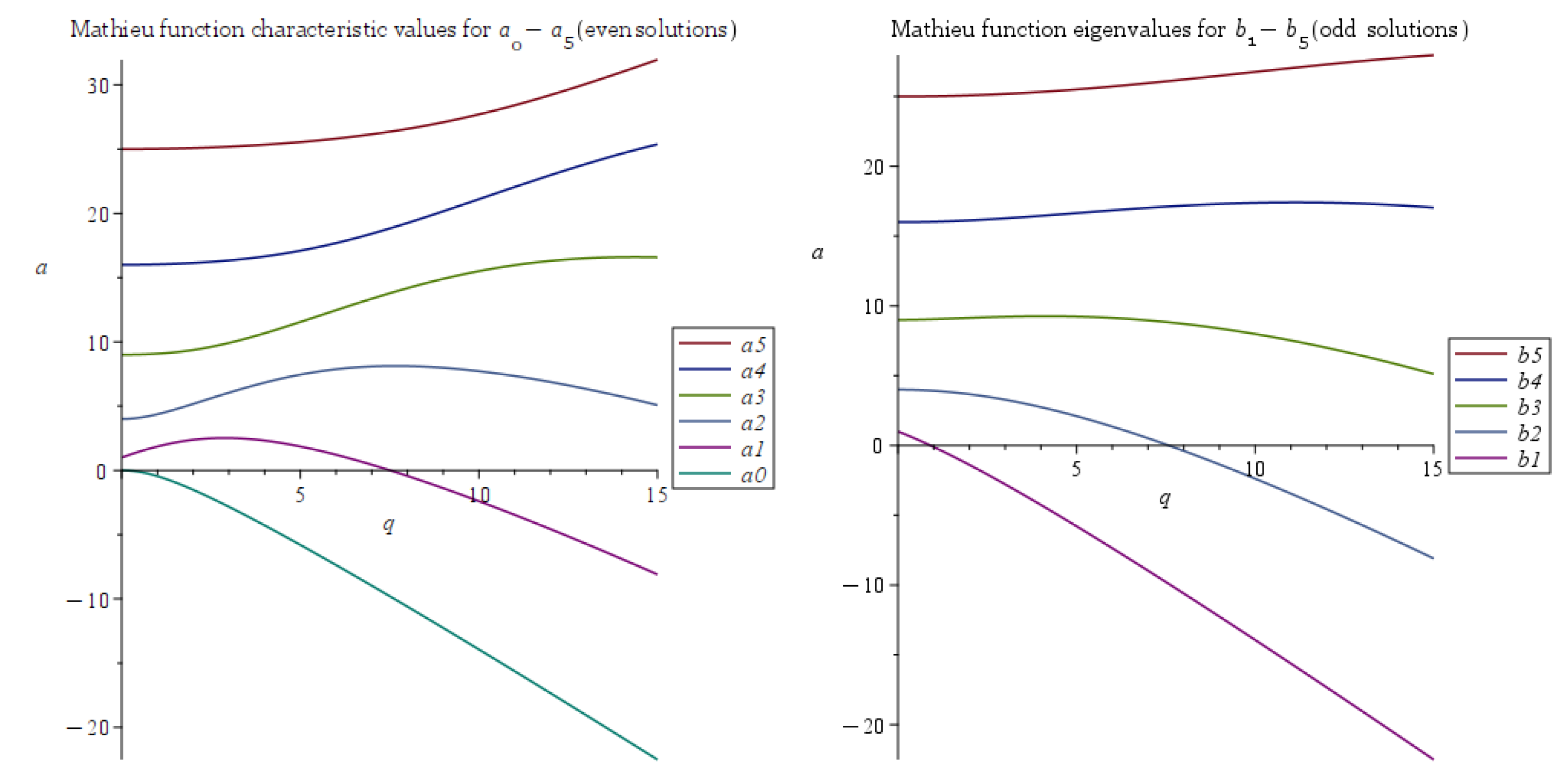
Figure 2.
The first image presents an extended view of the Mathieu equation stability diagram. The second image is focused on the first stability region delimited by the eigenvalues and , while the third image illustrates this stability region as shaded. The second stability region is delimited by the eigenvalues and .
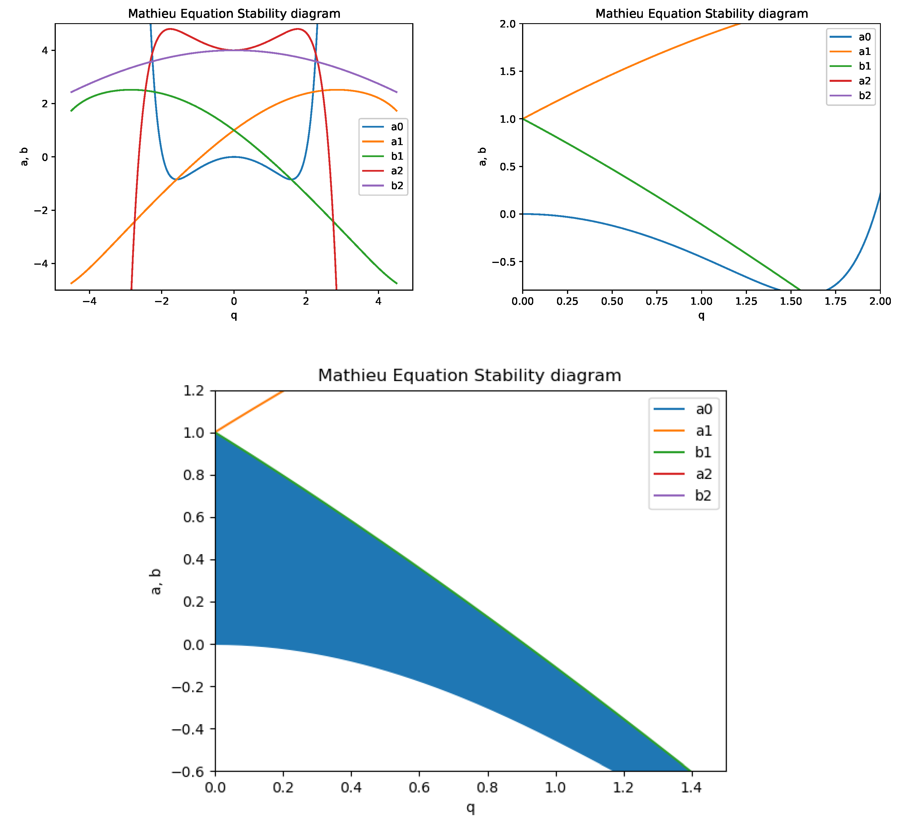
Figure 3.
The stability diagram for the combined (Paul and Penning) trap, where illustrate the frontiers of the stability diagram for the canonical Mathieu equation for axial motion. The frontiers of the stability domains for the radial trap motion are characterized by and . The c parameter is proportional with the cyclotronic frequency [20,28,32,132]. The central stability region is bounded by the characteristic curves of the eigenvalues and .
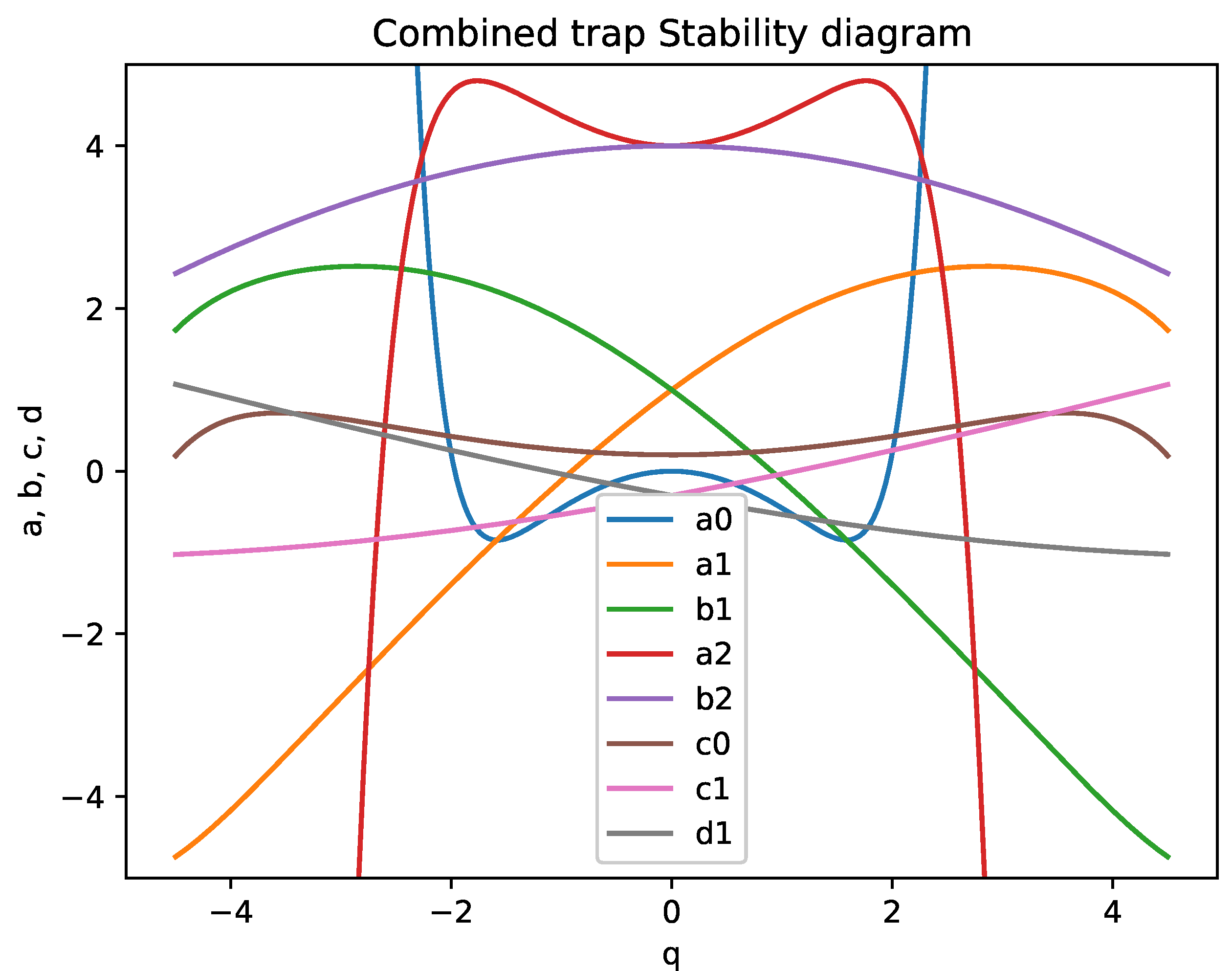
Figure 4.
The stability diagram for the 4th order nonlinear Paul trap. The first stability domains are characterized by the frontiers (filled in blue), respectively in case of the linear Mathieu equation () in eqs. (64 - 67).
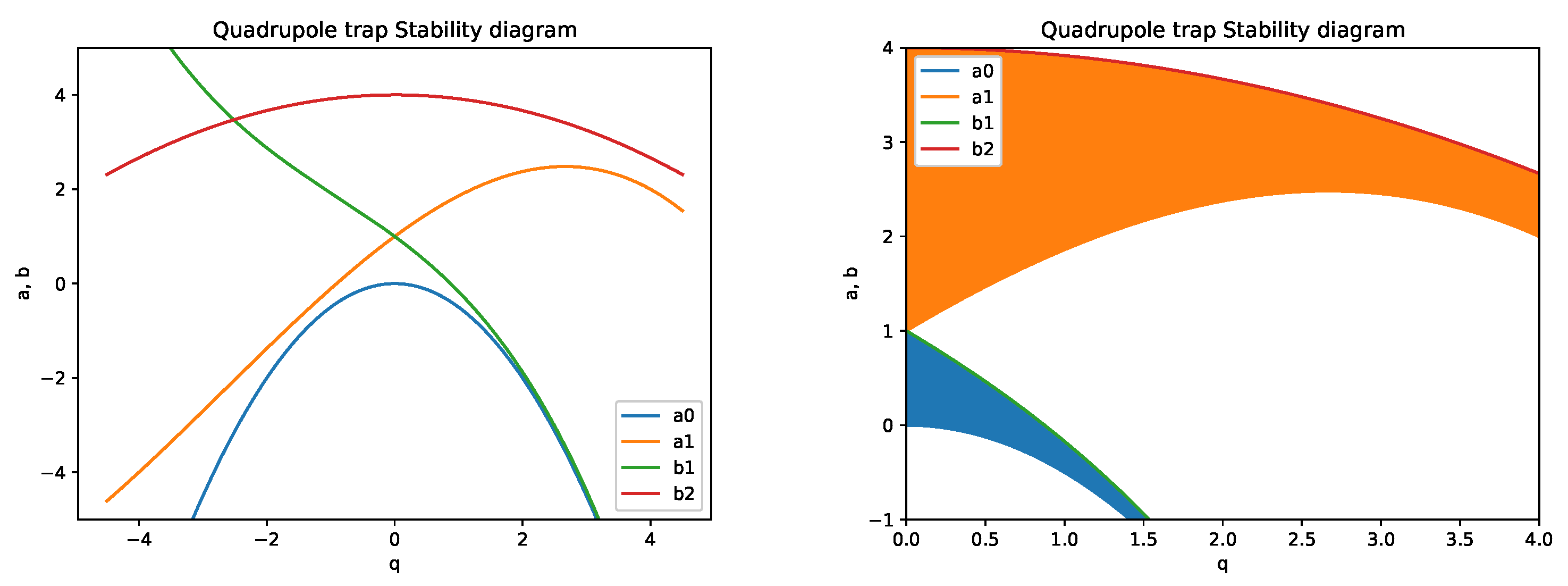
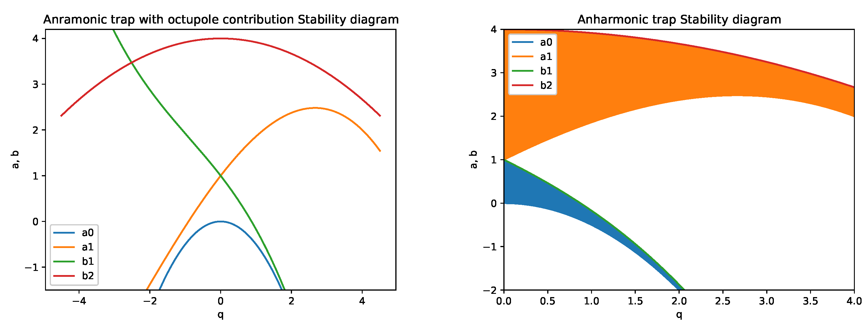
Disclaimer/Publisher’s Note: The statements, opinions and data contained in all publications are solely those of the individual author(s) and contributor(s) and not of MDPI and/or the editor(s). MDPI and/or the editor(s) disclaim responsibility for any injury to people or property resulting from any ideas, methods, instructions or products referred to in the content. |
© 2024 by the authors. Licensee MDPI, Basel, Switzerland. This article is an open access article distributed under the terms and conditions of the Creative Commons Attribution (CC BY) license (http://creativecommons.org/licenses/by/4.0/).
Copyright: This open access article is published under a Creative Commons CC BY 4.0 license, which permit the free download, distribution, and reuse, provided that the author and preprint are cited in any reuse.


