Optimal Investments in the Portfolia Yield Reactives (PYR)‡

Nikolaos Loukeris; Iordanis Eletheriadis

doi:10.20944/preprints202405.1065.v1

Submitted:

15 May 2024

Posted:

16 May 2024

Read the latest preprint version here

Abstract

We evolve our past models PYR, Loukeris, et al. (2016) to provide a competitive system whose infiltration of categorical information and fundamentals into advanced higher moments, supports a more objective Portfolio Selection, aided by Intelligent Computing. The system of Portfolia Yield Reactives (PYR) searches for hidden prototypes into big data of accounting and financial statements, restricting malicious patterns such as hoax, noise, manipulation, incorporated to a novel optimal portfolio selection method.

Keywords:

generalised feed forward networks

;

support vector machines

;

radial basis functions

;

genetic algorithms

;

regressions

;

integrated systems

;

portfolio selection

;

optimisation

Subject:

Business, Economics and Management - Finance

I. Introduction

The Epicurus measure of Eudaimonia, (serenity), as a dominant characteristic of his philosophy of Hedonism influenced the mathematical substratum two Millennia later. The quadratic investor preferences, and the returns distributions of Normal probability as given by the von Neumann-Morgenstern axioms of choice is the main approach in many portfolio selection models that follow the Markowitz’s mean-variance criterion. The empirical practice and the academic research clarified that neither of the two conditions hold, Merton (2009), as non-quadratic distributions are more efficient to describe investment patterns, and the returns are non-Normally Independently and Ideally Distributed. The Power Utility demonstrated a slight superior performance towards the Quadratic function, Loukeris et al. (2009). In support to that the implementation of higher moments than the fourth, establishes new qualities in the utility function behavior. Investors usually select positive skewness, derived of high profits from extreme positive events, Boyle and Ding (2005), against low kurtosis of low risk caused by extreme losses or profits in both sides of the distribution, Athayde and Flores (2003), Ranaldo and Favre (2003), Lai, Yu and Wang (2006). Loukeris et al. (2014a, 2015b, 2021), Loukeris (2021, 2022, 2023) remarked that advanced modeling is necessary to provide upgraded reliability to investor’s preferences under advanced higher moments. The m₁₀ HyperUltraKurtosis, in the Expected Utility, reflects more detailed forms of risk, eliminating hoax, noise or manipulation effects. The Hypothesis we make at this point is that the noise of systemic risk is provided by biased expectations or manipulation. We have had many cases that support this phenomenon: the Maddoff pryramids, the Toxic Bonds, the Greek Crisis, and many other cases of varying magnitude, that produce bubbles and instabilities.

Subrahmanyam (2007) rejects the theories of rational utility maximizers as an optimal behavioral tool as they are non-realistic, far from the markets.

The rest of this paper is organized as follows. Section 2 describes the theoretical part Section 3 analyses our model of portfolio selection in the Isoelastic Utility, the innovative limits of fundamentals in Intelligent Computing. Section 4 demonstrated the data. Section 5 supports the discussion of the results and Section 6 provides the conclusions.

II. Behavioral Parameters

In actual markets a high level of bias is endogenous on the portfolio, with limited diversification, Fidora, Fratzscher and Thimann (2006), Coeurdacier and Rey (2012). The risk differentials on stocks causes a partial effect in the cross-section of expected returns, Ang, Hodrick Xing and Zhang (2006), whilst data-mining is a significant aspect of empirical work. This loss avoidance agrees to the Epicouros (306 BC) philosophy of Hδονισμός (Hedonism-pursuit of pleasure), where the main goal of individuals is Hδονή – pleasure, through Aπονία – avoidance of unnecessary pain (risk). The loss averse investors with lesser emphasis to risk averse is the core of our model to the non-rational patterns of firm’s proximity to investor, time, period of the year, gender, etc.

III. Higher moments

The returns are non n.i.i.d. as the Efficient Market Hypothesis is insufficient to describe the complex real market phenomena. Subrahmanyam (2007), underlined that investors are interested mainly in their potential losses. The investors optimize their utilitarian preferences balancing fears and expectations to their earnings. Loukeris et al. (2014a, b), Loukeris et al. (2015b, a) introduced the 5^th moment of hyperskewness, the 6^th of hyperkyrtosis, the 7^th ultraskewness and 8^th ultrakurtosis. In this paper we introduce the 9^th of hyperultraskewness, and the 10^th of the hyperultrakurtosis on the Isoelastic Utility of the HARA family as:

Ut(R_t+1) = aE_t(R_t+1) – bVar_t(R_t+1) + cSkew_t(R_t+1) - dKurt_t(R_t+1) + eHypSkew_t(R_t+1) – fHypKurt_t(R_t+1) + gUltraSkew_t(R_t+1) –hUltraKurt_t(R_t+1) + iHypUltraSkew_t(R_t+1) –kHypUltraKurt_t(R_t+1)

(1)

Where

Kurt_t(R_t+1) = Var_t²(R_t+1)

(2)

HypKurt_t(R_t+1) = Kurt_t²(R_t+1) = Var_t⁴(R_t+1)

(3)

HypUltraKurt_t(R_t+1) = Kurt_t⁴(R_t+1) = Var_t⁸(R_t+1)

(4)

Where Ut(R_t+1) the overall utility the investor receives, a a proportion of mean return in the overall happiness of the investor, E_t(R_t+1) the expected return, b the proportion of risk to the utility measure, Var_t(R_t+1) the variance, c the proportion of skewness in the investor’s happiness, Skew_t(R_t+1) the skewness, d the proportion of Kurtosis, Kurt_t(R_t+1) the kurtosis of the investment, e the proportion of HyperSkewness, HypSkew_t(R_t+1) the HyperSkewness, f the proportion of HyperKurtosis, HypKurt_t(R_t+1) the HyperKurtosis of the investment, etc.

(2, 3, 4,) as a series of higher order moments can be extended to the desired level of analysis. The general form, Loukeris et al. (2015a, b) of the utility function is:

U_{t} (R_{t + 1}) = \sum_{λ_{ν} = 1}^{ω} {(- 1)}^{λ_{ν} + 1} \frac{a_{λ_{ν}}}{n} {\sum_{i = 1}^{n} (x_{i} - \sum \frac{x_{i}}{n})}^{n}

(5)

where λ_ν is the accuracy on investors utility preferences to risk, depending on the behavior, a_λν a constant on investors profile: a_λν = 1 for rational risk averse individuals, a_λν ≠ 1 for the non-rational, x_i the value of return i in time t. The Isoelastic Utility, of Constant Relative Risk Aversion, is on the risk averse investors:

U = \{\begin{matrix} \frac{W^{1 - λ} - 1}{1 - λ}, λ \in (0, 1) \cup (1, + \infty] \\ \log (x), λ = 1 \end{matrix}

(6)

where λ a measure of risk aversion, W the wealth. Loukeris et al. (2014a, b), Loukeris et al. (2015a, b) revealed that the Makowitz model can ease its essential assumption on the normally distributed prices.

IV. Methodology

A. Past models

The convex problem of quadratic utility maximization, Markowitz (1952), is a vague approach on the markets. Maringer and Parpas (2009) reformed it to:

\min_{x} f (x) = λ V a r (r_{p}) - (1 - λ) E (r_{p})

(7)

B. Problem Definition

Loukeris et al. (2014a, b), and Loukeris et al. (2015a, b), noticed the necessity of advanced higher to preferences to :

\min_{x} f (x) = λ υ_{γ} [b V a r_{t} (r_{p}) + d K u r t_{t} (r_{p}) + f H y p K u r t_{t} (r_{p})]

min_xf(x)=λυ_γ[bVar_t(r_p)+dKurt_t(r_p)+fHypKurt_t(r_p)+hUltraKurt_t (r_p)+kHypUltraKurt_t(r_p)]

(8)

υ_{γ} = 1 - ε_{τ}

(9)

r_{p} = \sum_{i} x_{i} r_{i}^{*}

(10)

where r_i^* stock’s i return on the efficient frontier- superior to the others, υ_γ the company’s financial health (binary: 0 to bankruptcy, 1 healthy), ε_τ the heuristic model output that is the evaluation result (binary: 0 healthy, 1distressed), x_i their weights.

The superiority of the selected stocks in the portfolio is:

i^* sup j if and only if R_t(i^*)>R_t(j), in:

Var_tR_t(i*)<Var_tR_t(j)

(11)

Kur_tR_t(i*)<Kur_tR_t(j)

(12)

HypKur_tR_t(i*)<HypKur_tR_t(j)

(13)

UltraKur_tR_t(i*) < UltraKur_tR_t(j)

(14)

HypUltraKur_tR_t(i*) < HypUltraKur_tR_t(j)

(15)

Stocks that don’t support all these superiority conditions are non-optimal, and removed from the optimal portfolio set, below the efficient frontier. Hence the Utility becomes, Loukeris et al. (2014a, b), Loukeris ae al. (2015a, b):

U_{t} (R_{t} (i)) = \sum_{λ_{ν} = 1}^{ω} {(- 1)}^{λ_{ν} + 1} \frac{a_{λ_{ν}}}{n} {\sum_{i = 1}^{n} (x_{i} - \sum \frac{x_{i}}{n})}^{n}

(16)

in

U_{t} (R_{t} (i^{*})) > U_{t} (R_{t} (x_{j}))

(17)

Being identical to

max_x E(U_P(w,λ)) (18)

As

E (U_{P} (w, λ)) = \max \{\frac{\sum_{i} {[1 + \exp (r_{i} x_{i})]}^{1 - \frac{υ_{γ}}{λ}}}{^{1 - \frac{υ_{γ}}{λ}}}\} / N

(19)

for Var_t²(r_p)=z

(20)

Var_t(R_t+1)=y

(21)

as z=y²=𝜎⁴ (22)

then

min_x f(x)=λv_yVar_t(r_p)[b+dz+fz²]

min_xf(x)=λυ_γ Var_t(r_p)[b+dz+fz²+hz⁴+kz⁶]

(23)

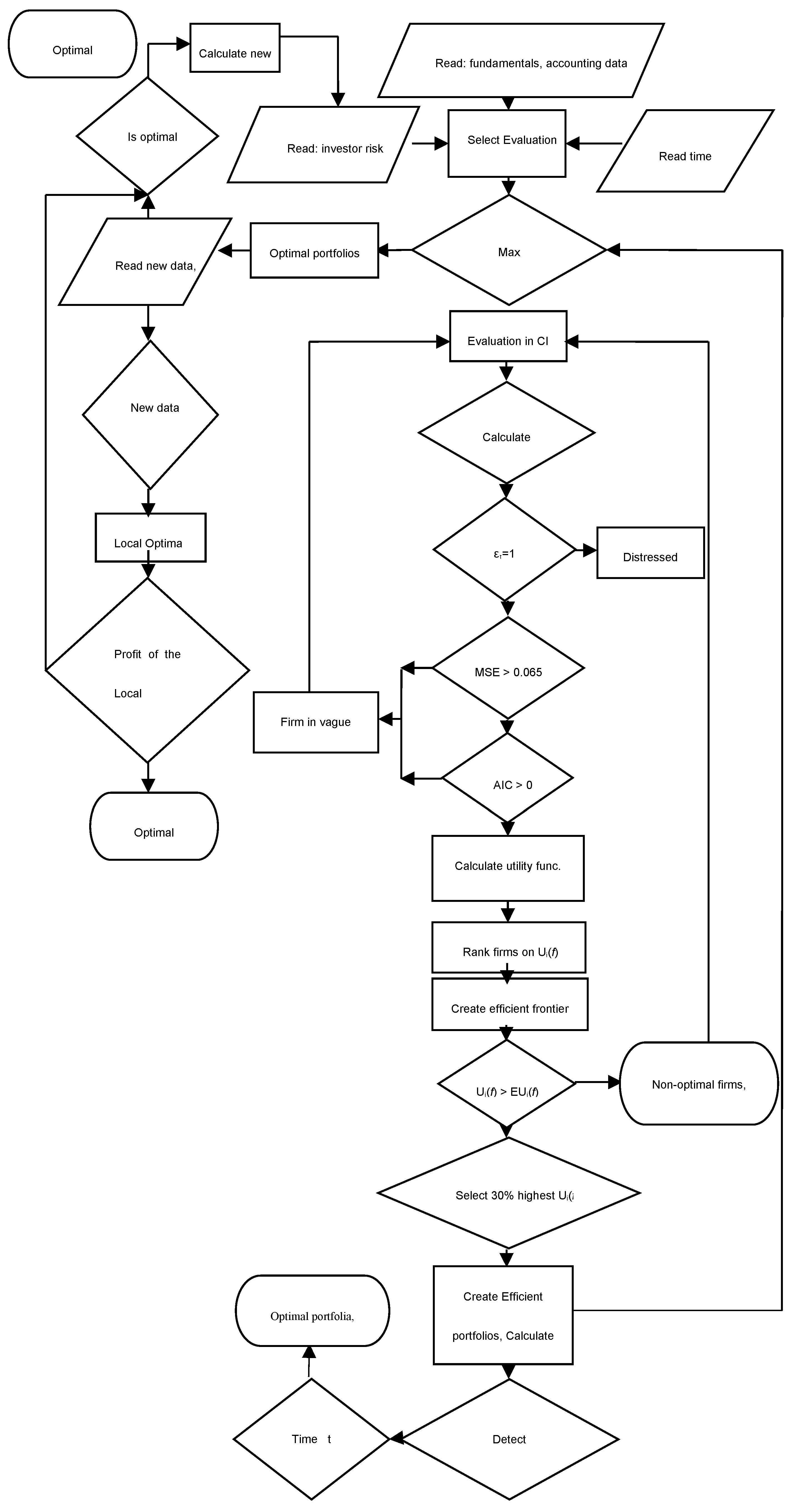
This non-convex problem, requires robust heuristics. Our novel contribution is that we extract hidden accounting and financial prototypes to a more detailed stock’s evaluation. Hoax and manipulation is an important risk to investors. (9) and (22) filter the distressed companies with no significant potentials from portfolios. The evaluation υ_γ, in (9) is more important than investor’s risk behavior, as they have a reverse influence in υ_γ/λ. The min_x f(x) in (8, 22) remarks a categorical, objective influence of a stock is more influential than subjective investors’ behavior. The flow chart of processes is in Figure 1.

C. The Portfolia Yield Reactives(PYR)

The Portfolia Yield Reactives model (PYR) is an advanced form of the integrated PI - Portfolio Intelligence model, Loukeris et al. (2015).

On the first step reads the fundamentals, the accounting data, the market prices and the preferred optimization period t.

Then it proceeds by selecting the initial method to evaluate the companies whose stocks are candidate in the portfolio. On this step the individual investor’s risk profile is given and the λ is selected for the Isoelastic utility, or it is re-calculated depending on the new market data.

If the optimal portfolio is in risk level λ then withhold, end.

Else Calculate new λ, read new λ.

If the new data on the selected stocks, or rest of the market stocks, and assets are different and include additional value,

Then there is Local Optimal Portfolio.

If the profit of the Local Optimal Portfolio on the current investment time horizon is acceptable

Then withhold, end.

Else re calculate portfolio.

On the next step, the system examines if this is the last firm to be examined, and if the condition for the optimal portfolio as an efficient portfolio is satisfied.

Else we proceed to the next of the initial evaluation that uses a Computational Intelligence model, to create two subsets: Subset A of the healthy companies, and Subset B of the distressed firms.

In the specific model we select the best network among the RBFs, the SVMs and the MLP, that is the hybrid SVM of 500 epochs optimized by GAs on the inputs only and Cross Validation, The ε_τ value is calculated (0, for the healthy and 1 for the distressed firms).

If ε_τ = 1 then the firm is distressed and it is removed, else if ε_τ = 0 the firm is healthy being candidate for the optimal efficient portfolio.

On the next step the U_t(R_t(_i)) the utility function of (14) is calculated per firm.

Next, firms are ranked according to their utility score.

Then, the Efficient Frontier is calculated.

Next, the firms with the higher utility score are selected into the efficient portfolio.

The sub-optimal firms as well as the non-optimal firms are revaluated with potential new data on the step 4 of Neural Nets evaluation, following all the steps.

Next, after the efficient portfolio is created, its Utility Function is calculated U_Pj(f).

Then, the optimal overall portfolio U*_Pj(f) whose utility is the maximum available, is detected, if possible, by all the available efficient portfolios utilities U_Pj(f) recorded in U*_Pj(f)> U_Pj(f).

The process stops when the time limit is reached and the PI has the optimal portfolio.

The key idea is to filter fraud and speculative noise that interfere on the price and disorient investors. Thus examining recent accounting entries and financial indexes we conclude on the realistic financial health of the firm. Then the actual healthy firms are selected, proceeding to the detection of efficient frontier and the creation of the optimal portfolio.

D. The processing phase

D.I The Generalized feedforward networks Neural Networks

Generalized feedforward networks are a generalization of the MLP such that connections can jump over one or more layers. Here you simply specify the number of layers, and the wizard will construct a MLP in which each layer feeds forward to all subsequent layers. In theory, a MLP can solve any problem that a generalized feedfoward network can solve. In practice, however, generalized feedforward networks often solve the problem much more efficiently. A classic example of this is the two spiral problem. Without describing the problem, it suffices

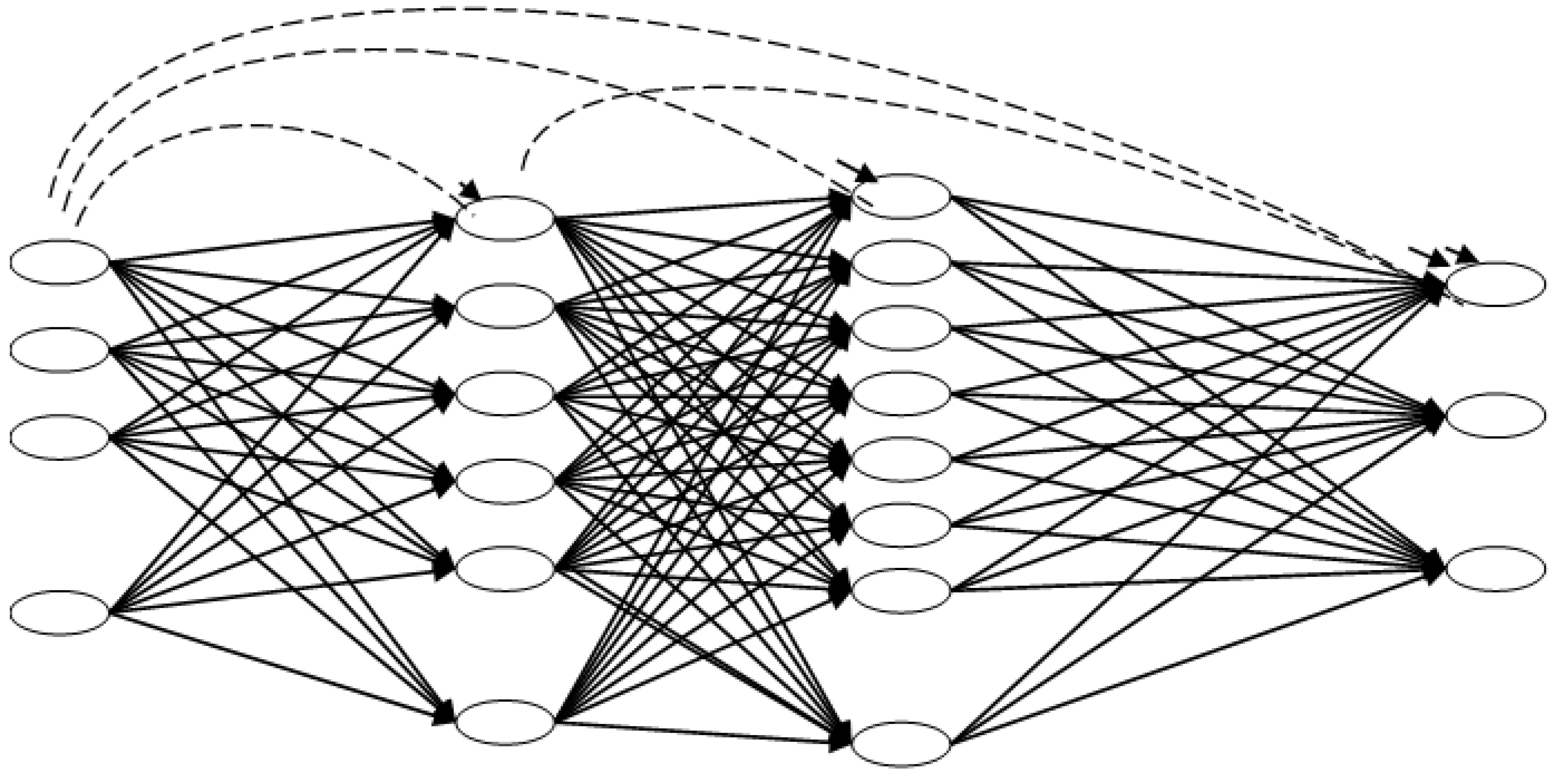
Figure 2. The Generalised Feed Forward – GFF Net

to say that a standard MLP requires hundreds of times more training epochs than the generalized feedforward network containing the same number of processing elements.

D.I.I The Generalized feedforward networks Hybrid Networks

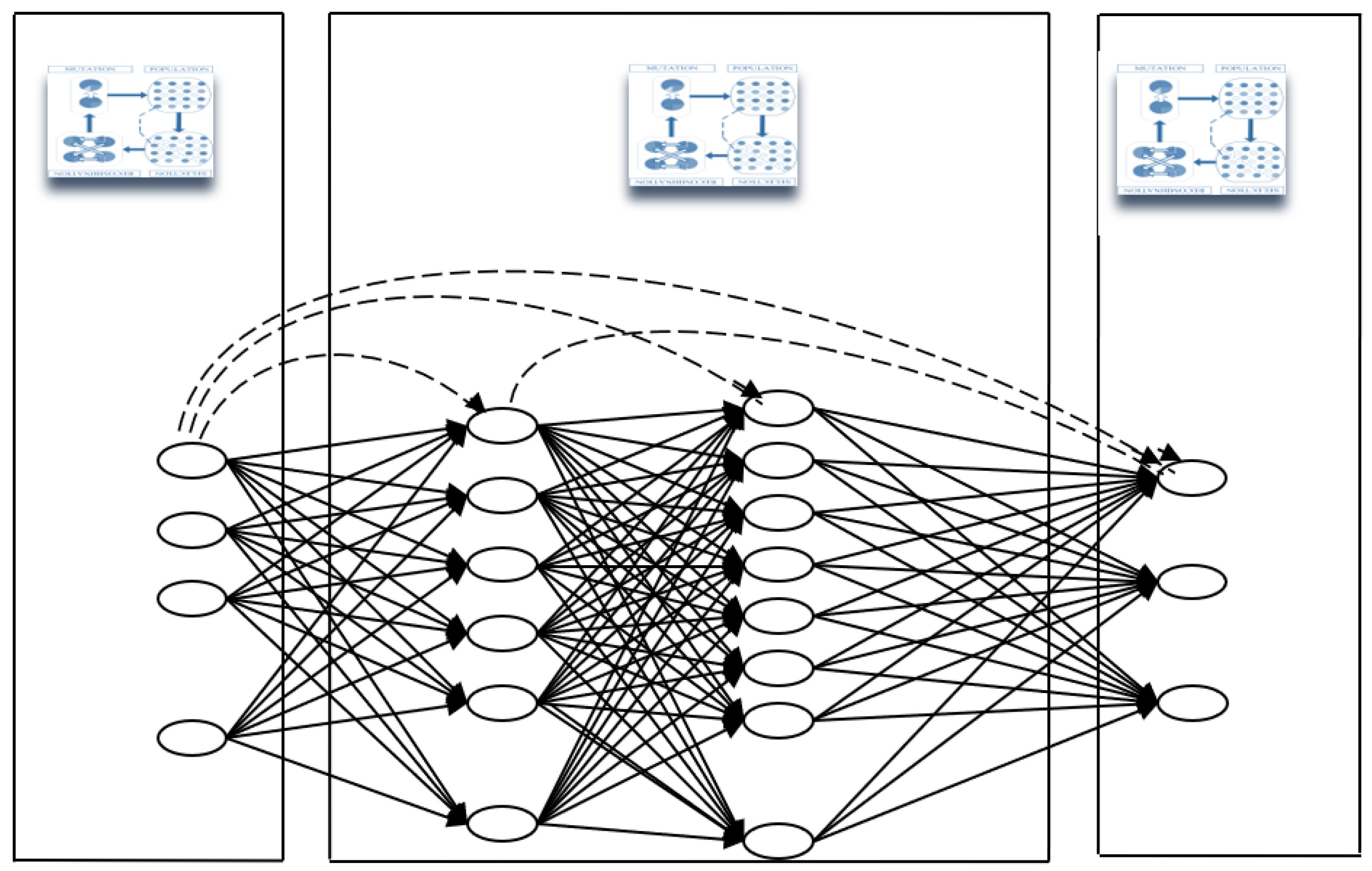
The Hybrid form of the GFFs can have Genetic Algorithms optimization in various layers, that advance the processing of certain parameters on the core of the neural GFF.

Figure 3. The Hybrid GFF Net of GA optimization and Cross Validation in all the layers .

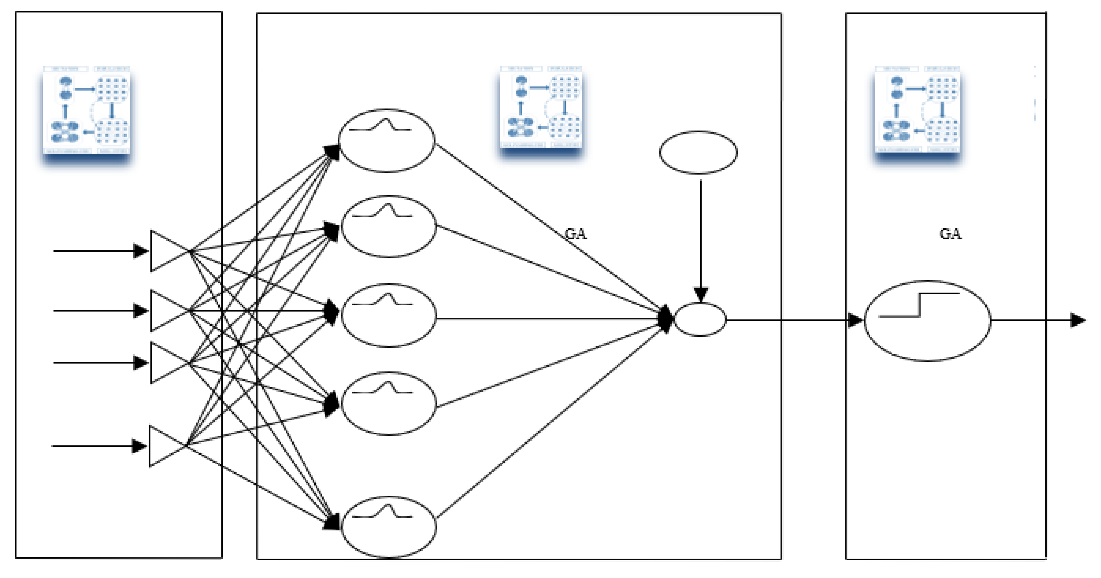
D.II The Hybrid Support Vector Machines

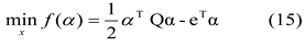
The Support Vector Machines-SVM, (Figure 1) produce general regression, and classification functions from a set of labeled training data, Cortes and Vapnik (1995), on a binary output, as input is categorical. Courtis (1978), noted that for instances x_i, i = 1,…l in labels y_i

\in

{1,−1}, SVM are trained optimising:

under: 0 ≤ α_i ≤ C, i= 1,…l, y^T α = 0,

where, e the vector of all 1, Q an lXl symmetric matrix of

Q_i,j=y_iy_jK(x_i, x_j), (16)

K(x_i, x_j) the kernel function, and C the upper bound of all variables. Unstable patterns are rejected by the SVM, as overfitted, receiving a statistically acceptable solution. These SVMs use the Adatron kernel algorithm under the NeuroSolutions software, mapping inputs to a high-dimensional feature space, separating data into their respective classes and isolating the inputs which fall close to the data boundaries. The converging system produces a few α_i ≠0, the support vectors, interacting with the closest boundary samples among classes. The Adatron kernel adjusts the RBFN in an optimal margin, and prunes the RBF net so that its output for testing is:

f(x)=sgn[∑g_iα_iG(x – x_i, 2𝜎²) - b], (25)

i

\in

support vectors. None of the 16 inputs has a predefined significance to the hybrid genetic SVMs. The GAs select important inputs, demanding a multiple training of the network to define them provide the minimum error. In accordance to Min, Lee, and Han, (2006), where optimisation emphasizes on the feature subset and the SVM parameters, we move forth examining multiple hybrid SVM models. Specifically the GAs were elaborated in different hybrids: i) the SVM inputs only, ii) the SVM outputs only, and iii) both the inputs and outputs. Batch learning was preferred on the weights after the presentation of the whole training set. All models were tested on 500 and 1000 epochs respectively, to optimize the iterations number upon convergence. Min, Lee, and Han, (2006), performed the feature selection either on the filter, or the wrapper approach. The filter approach is computationally more efficient, but the wrapper approach, although slower, selects the features more optimally. In the bankruptcy prediction problem, feature subset selection plays an important role in the performance of prediction. Furthermore, its importance increases when the number of features is large.

This paper uses the wrapper approach to select the SVM optimal training.

Figure 2. The Support Vector Machines.

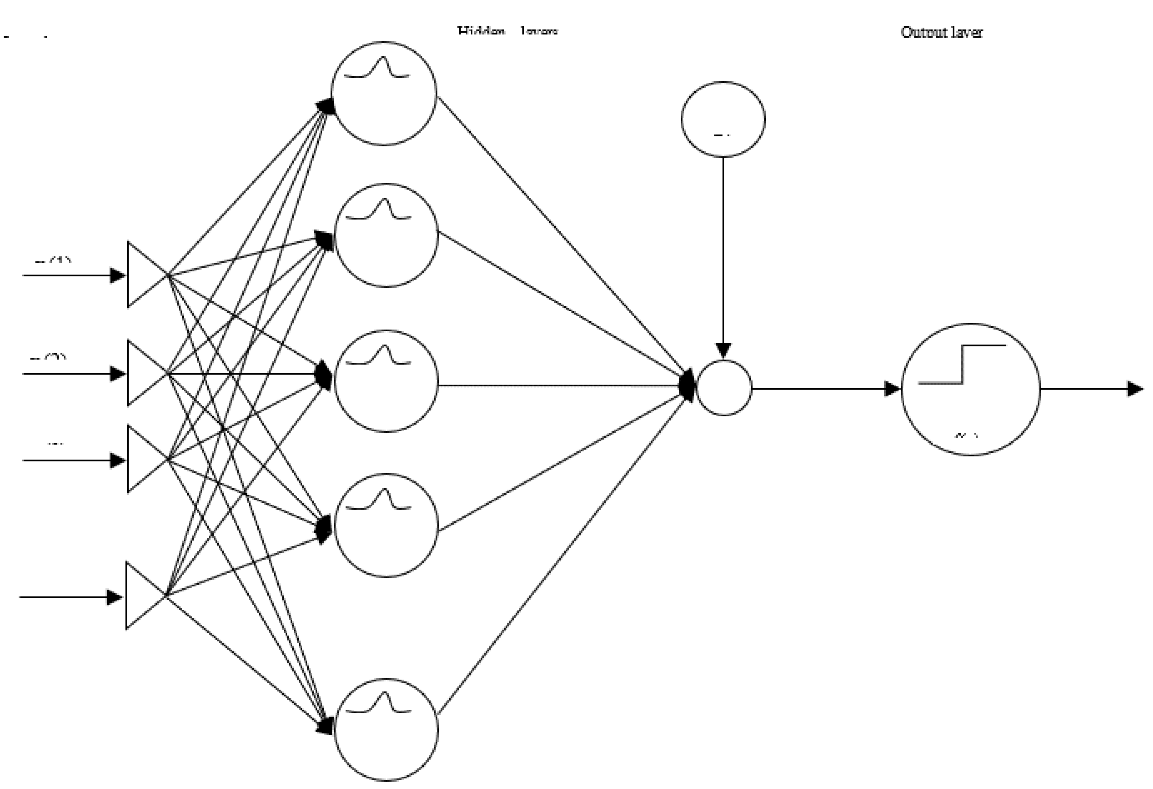
Figure 3. The Hybrid Genetic Support Vector Machines optimized in GAs on all the layers with or without Cross Validation.

mal feature subset in GA. The increase function is selected to terminate training under the Cross Validation set when its MSE increases, avoiding the overtraining, whilst best training weights are loaded on the test set. The GA solved the optimal values problem in a) number of neurons, b) the Step size, and c) the Momentum Rate, requiring a multiple training of the network to conclude the lowest error mode. In case of the models with GA on the output layer, they optimized the value of the Step size and the Momentum. The higher number of epochs allowed iterations to provide more thorough analysis on the network, the overall classification on these SVM models was excellent taking as benchmark the bank experts initial opinion, with fine performance in almost all the model parameters, that failed to reduce overtraining hazard in almost all different SVM hybrid or SVM models, questioning the models independence, and impartiality. Overall the Hybrid SVM of 1000 epochs GA optimization on the inputs and Cross Validation converged optimally in classification and performance terms, a significant overtraining hazard but in excess computation time. The Hybrid SVM of 500 epochs of inputs Genetic Algorithms optimization almost similar qualities in less time, and the third rank is given to the SVM of 1000 that in all sets remained very reliable on the highest over fitting hazard but a very fast computational time. These models are quite useful to all profiles of investors putting emphasis either in accuracy, or speed, whilst the over fitting aspect must be considered. A comparative analysis of the SVM results, Table 1, to the MLP, Loukeris and Eleftheriadis, (2012a), that is a basic Neural Network, clearly shows the higher classification capabilities of the SVM models that face the criticism of partiality on the models behavior towards the supervisor, and the underperformance of the MLP that was last in classification and efficiency, but didn’t face questions on integrity.

The overall results Loukeris and Eleftheriadis (2013), revealed that the Hybrid SVM of 500 epochs, inputs GA and Cross Validation, had a fine classification, with high differences on the CV classification regarding the distressed results, the lowest Error on MSE and CV MSE at 0.023 and 0.309 respectively, low NMSE, low percentage error, fine fitness to the data at 0.999 and 0.949 on the CV, significant overtraining hazard as AIC was 21524.30 and 23409.93 on the CV, requiring an extended time of 26 hours 56 minutes 14 sec.

The second place was taken by the SVM of 1000 epochs, excellent classification and performance, as MSE was the second lower at 0.035, NMSE at 0.066, percentage error at 4.85% similarly, in a very high partiality exposure as AIC was 23016.76, converging almost instantly in 4 minutes 11 seconds. Finally on the third place the SVM of 500 epochs that had a fine classification, almost fine performance but in high overtraining hazard in partiality as AIC reached 23073.68 and an almost instant processing time of 1 min 52 sec.

D.III The Hybrid Radial Basis Functions

The RBFs are linear models of regressions, classifications and time series predictions in supervised learning. The set of examples, contains the independent variable, sensitive to noise, and the dependent one. An RBF net is in Figure 2. The importance of each financial index out of the 16 inputs in the RBF hybrid nets is unknown to the model and Genetic Algorithms investigate them. Each model is trained multiple times to define the inputs combination of the lowest error. Genetic Algorithms were implemented in different hybrid models:

I.: on the inputs layer only,
II.: on the inputs and outputs layers only,
III.: in all the layers and cluster centers,
IV.: in all the layers and cluster centers with cross validation,

in different topologies. Batch learning was also selected to update the weights of the hybrid neuro-genetic RBFs, after the entire training set is presented. The competitive rule was the ConscienceFull function in Euclidean metric as the conscience mechanism keeps a count on how often a neuron wins the competition, and enforces a constant wining rate across the neuron s. There were 4 neuron s per hidden layer, using the TanhAxon transfer function, on the Momentum learning rule. Genetic Algorithms resolved the problem of optimal values in a) neurons, b) step size, c) momentum rate, and d) cluster

Figure 6. The Radial Basis Function Networks.

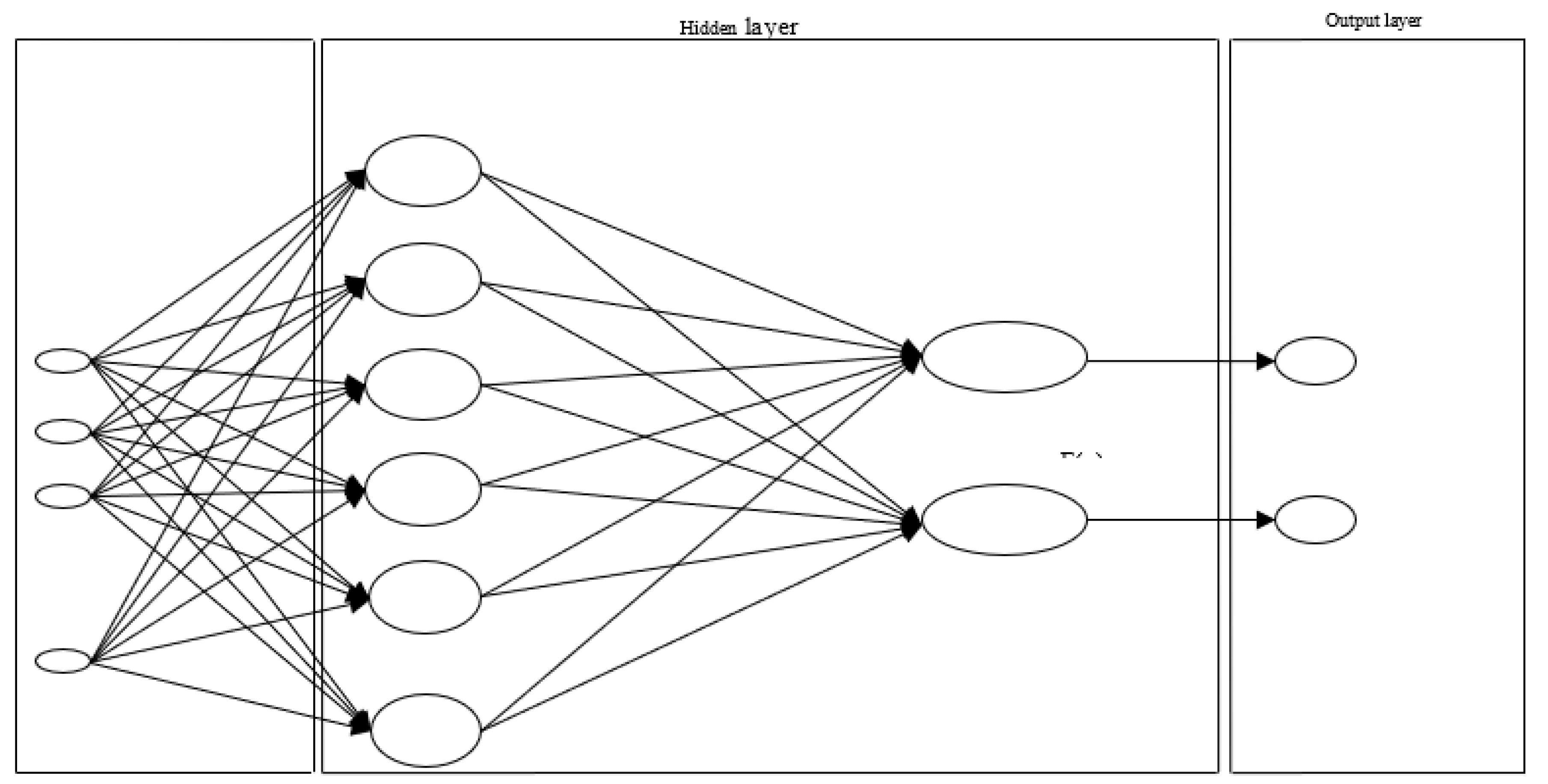
centers. RBF nets require multiple training to obtain the lowest error. The output layer elaborated Genetic Algorithms in some hybrids optimizing the Step size and the Momentum.

The overall performance, Loukeris, Eleftheriadis and Livanis (2014a), was given by the Hybrid RBF on GA optimisation into inputs and outputs only of 3 layers where 97.24% and 72.48% of the companies converged in as healthy and distressed respectively, the fitness of the model to the data was high at r 0.925 whilst errors remained low at MSE 0.116, NMSE at 0.393, in error 9.039% on a moderate Akaike criterion, in a short computing time of 5 hours 48 minutes 56 s.

The second place was given to the Hybrid RBF of GAs in all layers if no hidden layers where98.15% of healthy and 60.09% of distressed companies were correctly classified, in a fine fitness to the data at 0.815 in medium MSE, NMSE, proportional errors, medium AIC signifying statistical non-impartiality, in a quick processing time of 5 hours 2 min. 28 s.

V. Data

Data were produced by 1411 companies from the loan department of a Greek commercial bank, with the following 16 financial indices:

1) EBIT/Total Assets,

2) Net Income/Net Worth,

3) Sales/Total Assets,

4) Gross Profit/Total Assets,

5) Net Income/Working Capital,

6)Net Worth/Total Liabilities

7)Total Liabilities/Total assets,

8) Long Term Liabilities/(Long Term Liabilities + Net Worth),

9)Quick Assets/Current Liabilities

10)(Quick Assets-Inventories)/Current Liabilities,

11)Floating Assets/Current Liabilities,

12)Current Liabilities/Net Worth,

13) Cash Flow/Total Assets,

14)Total Liabilities/Working Capital,

15)Working Capital/Total Assets,

16) Inventories/Quick Assets,

and a 17th index with initial classification, done by bank executives. Test set was 50% of overall data, and training set 50%. Multiple combinations were chosen to detect the performance of SVM and RBF Networks:

A.: SVM of 500 or 1000
B.: SVM of 500 epochs and GA on inputs
C.: SVM of 1000 epochs and GA on inputs
D.: SVM of 500 epochs and GA on outputs
E.: SVM of 1000 epochs and GA on outputs
F.: SVM of 500 epochs and GA in all layers
G.: SVM of 1000 epochs and GA in all layers
H.: SVM of 500 epochs and GA on inputs, and Cross Validation
I.: SVM of 1000 epochs and GA on input, and Cross Validation
J.: RBF Neural Nets,
K.: RBF hybrids in inputs GA,
L.: RBF hybrids in inputs and outputs GA,
M.: RBF hybrids of GA in all layers,
N.: RBF hybrids of GA in all layers and Cross Validation,

Figure 7. Hybrid Radial Basis Function in GAs optimisation on input and output layers only.

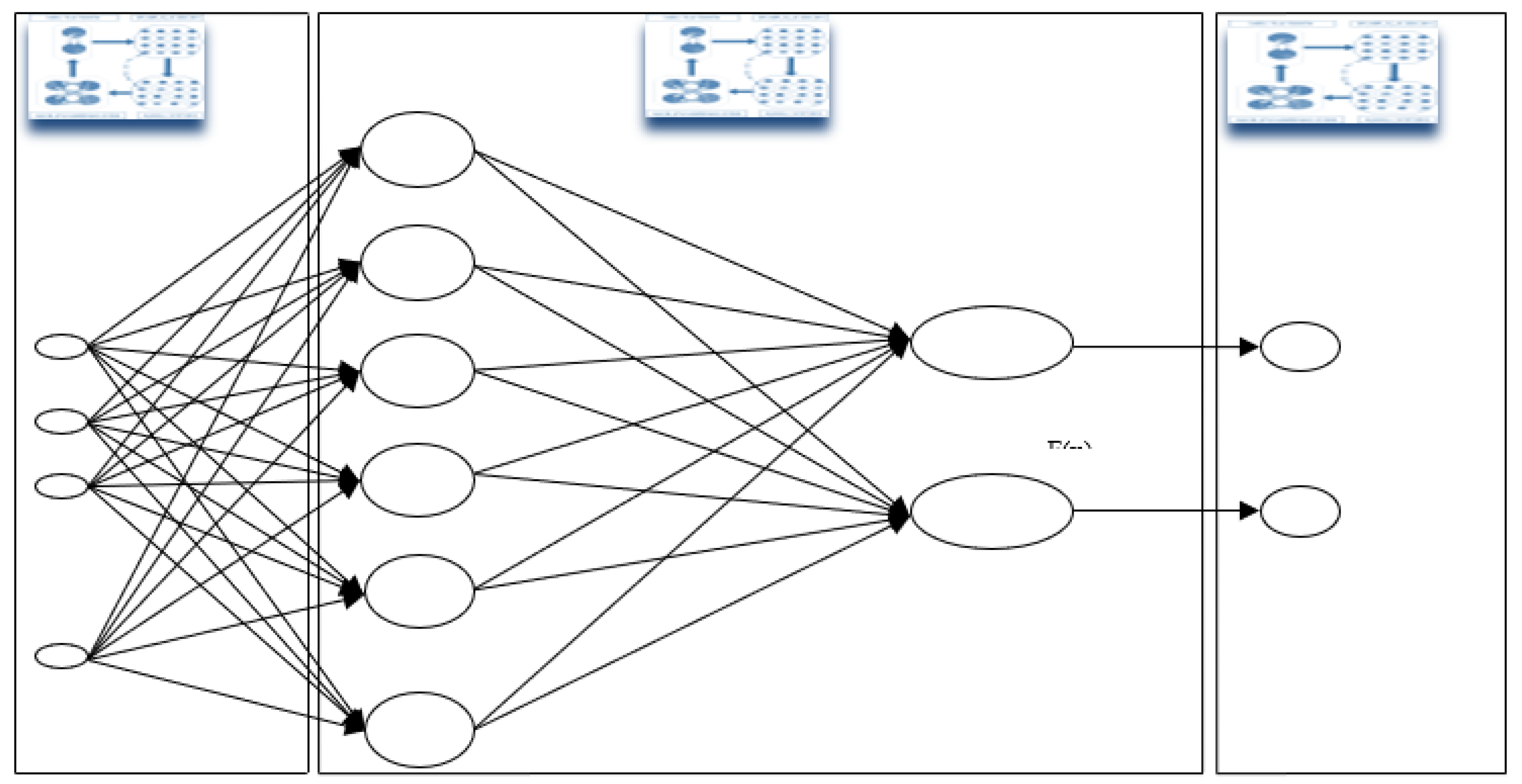
Table 1. Overall ranking of the optimal GFF models.

Models		Active Confusion Matrix				Performance
Layers		0→0	0→1	1→0	1→1	MSE	NMSE	r	%error	AIC	MDL
GFF input-output GA	1	98,90	1,085	11,465	88,52	0,072	0,1705	0,908	5776	-1907,09	-1796,44	55' 18''
GFF GA all	3	97,14	2,845	17,885	82,10	0,128	0,304	0,834	8,3435	40259,12	284,345	2h 44' 43''
	1	97,56	2,425	18,805	81,18	0,133	0,3155	0,8275	8,2435	-723,475	-271,82	1h 38' 53''
GFF GA all,	7	96,64	3,35	19,26	80,73	0,136	0,323	0,825	9,119	1541,07	3429,31	7h 42' 32''
CV		98,32	1,67	29,355	70,63	0,149	0,3535	0,8125	7,073	1608,295	3495,495
GFF NN	1	97,73	2,26	21,095	78,89	0,138	0,328	0,8215	9,6755	-1225,82	-1111,95	4''
GFF NN, CV	8	98,23	1,755	26,14	73,85	0,143	0,3385	0,814	9,2845	709,44	2041,355	14,5''
CV		98,23	1,755	26,14	73,85	0,143	0,3385	0,814	9,2845	709,44	2041,355
GFF GA inputs	10	97,98	2,005	26,6	73,16	0,144	0,341	0,8125	9,4695	1219,39	2873,695	1h 27' 44''
GFF GA all	8	98,57	1,42	26,6	73,39	0,140	0,3295	0,8215	8,329	1262,655	2959,695	5h 59' 49''
GFF GA all,	1	97,98	2,005	24,305	75,68	0,145	0,343	0,8105	8,646	-1219,07	-1126,3	1h 48' 31''
CV		98,4	1,59	24,765	75,22	0,139	0,3305	0,8215	8,6865	-1242,55	-1149,79
GFF NN	10	98,65	1,34	31,185	68,80	0,147	0,348	0,8105	8,454	1557,505	3419,165	9,5''

Table 2. The SVMs optimal results, and the MLP, Loukeris and Eleftheriadis (2012a), Loukeris et al. (2013).

Neural Network	Active Confusion Matrix					Performance						Time
Layers	0→0	0→1	1→0	1→1	MSE	NMSE	r	%error	AIC		MDL
SVM 500 epochs	100	0	0	100	0.035	0.072	0.999	5.43674	23073.68	39305.45		1’52’’
SVM 1000 epochs	100	0	0	100	0.035	0.066	0.999	4.85737	23016.76	39248.53		4’11’’
Hyb.SVM 500 ep.GAinput	100	0	0	100	0.045	0.086	0.999	6.55585	16159.80	27896.09		14h39’31’’
Hyb.SVM 500 epGAoutput	100	0	0	100	0.065	0.125	0.999	6.80503	23457.92	39689.69		1h 07’ 34’’
Hyb.SVM 1000 epGAoutput	100	0	0	100	0.049	0.095	0.999	6.23541	23253.32	39485.09		4h23’35’’
Hyb.SVM 500 ep GA in, Cro. Val.	100	0	0	100	0.023	0.045	0.999	4.01337	12044.20	21524.30		26h 56’ 14’’
	94.29	5.69	22.01	77.98	0.309	0.591	0.949	12.7284	13931.09	23409.93
Hyb. SVM 1000 ep GA out., C.V.	100	0	0	100	0.098	0.505	0.999	6.13446	23292.73	39540.51		5h 38’ 12’
	94.63	5.36	24.31	75.68	0.522	0.679	0.971	1.71621	24663.75	40911.52
Hyb. SVM 500 ep GA All, C.V.	100	0	0	100	0.091	0.175	0.999	9.06724	12375.85	21401.51		21h 16’ 32’’
	95.88	4.10	25.22	74.76	0.541	1.037	0.983	25.1262	13646.24	22672.40
MLP N. N. 1	100	0	98.62	1.37	0.418	0.989	0.107	19.4320	-468.25	-374.8		15’’

Table 3. RBFs Overall Optimal Results, Loukeris, Eleftheriadis and Livanis (2014a).

Hybrid Networks		Active Confusion Matrix					Performance					Time
Layers		0→0	0→1	1→0	1→1	MSE	NMSE	r	%error	AIC	MDL
RBF input-output GA	3	97.24	2.76	27.52	72.48	0.166	0.393	0.925	9.039	672.93	1912.74	5h48’56’’
RBF GA	0	98.15	1.85	39.91	60.09	0.188	0.445	0.815	13.009	37.12	820.831	5h 02’28’’
RBF inputs GA	0	97.73	2.26	46.32	53.67	0.219	0.519	0.791	12.383	282.78	1154.02	4h 19’42’’

Table 4. Overall Optimal Results on GFFs, SVMs, RBFs MLPs, Loukeris and Eleftheriadis (2012a), Loukeris et al. (2013), Loukeris et al.(2014a).

Neural Network	Active Confusion Matrix					Performance							Time
Layers	0→0		0→1	1→0	1→1	MSE	NMSE	r	%error		AIC	MDL
Hybrid SVM 500 ep GA in, C. V.	100		0	0	100	0.023	0.045	0.999	4.0133	12044.20		21524.3	26h 56’ 14’’
	94.29		5.69	22.01	77.98	0.309	0.591	0.949	12.728	13931.09		23409.9
SVM 500 epochs	100		0	0	100	0.035	0.072	0.999	5.4367	23073.68		39305.4	1’52’’
SVM 1000 epochs	100		0	0	100	0.035	0.066	0.999	4.8573	23016.76		39248.5	4’11’’
HybridSVM 500 ep GA input	100		0	0	100	0.045	0.086	0.999	6.5558	16159.80		27896.0	14h39’31’’
HybridSVM 1000 ep GA output	100		0	0	100	0.049	0.095	0.999	6.2354	23253.32		39485.0	4h23’35’’
HybridSVM 500 ep GA output	100		0	0	100	0.065	0.125	0.999	6.8050	23457.92		39689.6	1h 07’ 34’’
Hybrid SVM 1000 ep.GA outCV	100		0	0	100	0.098	0.505	0.999	6.1344	23292.73		39540.5	5h 38’ 12’
	94.63		5.36	24.31	75.68	0.522	0.679	0.971	1.7162	24663.75		40911.5
Hybrid SVM 500 ep GA All,CV	100		0	0	100	0.091	0.175	0.999	9.0672	12375.85		21401.5	21h 16’ 32’’
	95.88		4.10	25.22	74.76	0.541	1.037	0.983	25,126	13646.24		22672.4
RBF input-output GA 3	97.24		2.76	27.52	72.48	0.166	0.393	0.925	9.039	672.93		1912.74	5h48’56’’
GFF input-output GA 1	98,90		1,08	11,46	88,52	0,072	0,170	0,908	5776	-1907,09		-1796,44	55' 18''
GFF GA all 3	97,14		2,84	17,88	82,10	0,128	0,304	0,834	8,3435	40259,12		284,345	2h 44' 43''
GFF GA all1	97,14		2,845	17,88	82,10	0,128	0,304	0,834	8,3435	40259,12		284,345	1h 38' 53''
RBF GA All 0	98.15		1.85	39.91	60.09	0.188	0.445	0.815	13.00	37.12		820.831	5h02’28’’
RBF inputs GA 0	97.73		2.26	46.32	53.67	0.219	0.519	0.791	12.383	282.78		1154.02	4h19’42’’
MLP N. N. 1		100	0	98.62	1.37	0.418	0.989	0.107	19.432	-468.25		-374.8		15’’

This model has a wider approach on the stock market assets. Due to limitations of data we also examined private companies. The investor can select a variety of assets (common, preferred, private, bonds, treasury bills).

VI. Results

A comparison of all the outcomes would clearly rank first among all the SVM, RBF and MLP models the hybrid SVM of 500 epochs optimized by GAs on the inputs only and Cross Validation, in a 100% classification in the correct classified assets, a fitness of the model to the data r 0.999 of the lowest error in MSE at 0.023, NMSE 0.045, overall error 4.01% but a significant partiality of Akaike 12044.20, extended training time of 26 hours 56 minutes 14 seconds. Time is not an issue for the trained model, as the cross validation reduces overfitting. The main vulnerability of AIC that reveal partiality and dependence of its performance by the Desired Classification as given by human experts. But this is of lower significance as the CV set was quite good, in 94.29% correct classifications on the healthy companies, 77.98% on the distressed in a medium error of 0.309 in MSE, 0.591 on NMSE, 12.72% on overall error.

The second rank was taken by the SVM of 500 epochs in excellent classification, performance and a very fast time, exposed to overfittting and partiality.

Third was ranked the SVM of 100 epochs in excellent outcomes of classification, performance, and time, in the same weaknesses of overfitting and partiality.

The RBFs underperformed in classification, but with a very high fitness 0.925, in high error and AIC as well. The other RBF models and the MLP significantly underperformed ranked last than the SVMs.

The integrated PYR model thus will have robust classifiers depending the need of the users, the depth of accuracy, the form of the data. As an overall portfolio selection system it eliminates market manipulation incorporating the fundamentals as comparative parameter to the stock return in the markets, and also introduces more processes of re-evaluation for the optimization of the investment portfolio.

VII. Conclusions

The integrated model Portfolia Yield Reactives - PYR, offers an advanced analytical processing in the Decentralised Finance – De.Fi., supporting the real time portfolio selection problem. The main advantage of this system is that by extracting hidden patterns it tries to avoid manipulation, and speculation games. The hybrid SVMs nets have a promising performance of high calibration that can allow them to be a part of this model or its future upgrades. The hybrid SVM of 500 epochs optimized by GAs on the inputs only and Cross Validation although it provides a perfect performance and classification, in a restricted processing time, demonstrates a significantly higher partiality, as the SVM of 500 epochs despite its slight underperformance demonstrates robust qualities that suffer from overfitting and partiality.

Hence the SVM models offer perfect classification, on condition for financial data, than the RBF that had quite lower performance with much more weaknesses or even worse the GFFs.

Funding

This research received external funding by the ELKE Fund of the Universities of Macedonia and West Attica.

Conflicts of Interest

The authors declare no conflict of interest.

References

Ang, A. Hodrick R., Xing Y., and X., Zhang (2006), The Cross-Section of Volatility and Expected Returns, Journal of Finance, vol LXI, No1, February.
Athayde, G. , and R. Flores, (2003), Incorporating skewness and Kurtosis in portfolio optimization: a multidimensional efficient set. In: Satchell, S., Scowcroft, A. (eds.) Advances in Portfolio Construction and Implementation, pp. 243–257.
Coeurdacier N., and H., Rey (2012), Home Bias in Open Economy Financial Macroeconomics, Journal of Economic Literature, 51(1), 63-11. [CrossRef]
Cortes C. and Vapnik V. (1995), Support-vector network-. Machine Learning, 20:273–297, in Portfolio Selection, Journal of Global Optimization, Volume 43, Numbers 2-3, March.
Courtis, J. K. , (1978), Modeling a Financial Ratios Categoric Framework, J. Bus.Fin. & Acc., 5(4): 371-386. [CrossRef]
Fidora, M. Fratzscher M., and C., Thimann (2006), Home Bias in Global Bond and Equity Markets – The role of real Exchange Rate Volatility, European Central Bank, Working Paper Series 685 , October.
Lai, K.K. Yu, L., and S. Wang, (2006), Mean-variance-skewness-kurtosis-based portfolio optimization. First International Multi-Symposiums on Computer and Computational Sciences (IMSCCS’06) Vol. 2 , 292–297.
Loukeris, N. , Donelly D., Khuman A., Peng Y., (2009), A numerical evaluation of meta-heuristic techniques in Portfolio Optimisation, Operational Research, Volume 9(1), ed. Springer Verlang. [CrossRef]
Loukeris, N. and I.Eleftheriadis, (2012a), Bankruptcy Prediction in Hybrids of Time Lag Recurrent Networks with Genetic optimisation, Multi Layer Perceptrons Neural Nets, and Bayesian Logistic Regression, Proceedings of the International Summer Conference of the International Academy of Business and Public Administration Disciplines (IABPAD), ISSN 547-4836 Library of Congress, Honolulu, Hawaii, USA (August 1- 5) - Research Paper Award.
Loukeris, N. and I.Eleftheriadis, (2013), A novel Approach on Hybrid Support Vector Machines into Optimal Portfolio Selection, Proceedings of the IEEE International Symposium on Signal Processing and Information Technology, December 12-15, Athens, Greece. [CrossRef]
Loukeris, N. Eleftheriadis I. and E. Livanis (2014a), Optimal Asset Allocation in Radial Basis Functions Networks, and hybrid neuro-genetic RBFΝs to TLRNs, MLPs and Bayesian Logistic Regression, World Finance Conference, Venice, Italy July 1-3.
Loukeris, N. Eleftheriadis I. and E. Livanis (2014b), Portfolio Selection into Radial Basis Functions Networks and neuro-genetic RBFN Hybrids, IEEE 5^th International Conference on Information, Intelligence, Systems and Applications IISA , July 7-9, Chania Greece.
Loukeris, N. Boutalis, Y.,; Livanis S., Arampatzis, A., and L. Maltoudoglou, (2015a), Hybrid Jordan Elman nets in portfolio selection, IEEE 6^th International Conference on Information, Intelligence, Systems and Applications IISA, Corfu, Greece, July 6-8, pp 1-6.
Loukeris, N. Boutalis, Y.,; Livanis S., Arampatzis, A., and L. Maltoudoglou, (2015b), Computational intelligence in optimal portfolio selection - The PI model, IEEE 6^th International Conference on Information, Intelligence, Systems and Applications IISA, Corfu, Greece, July 6-8, pp 6-12.
Loukeris N., Bekiros S., and Eleftheriadis I., (2016), The Portfolio Yield Reactive (PYR) model, IEEE 6th International Conference on Information, Intelligence, Systems and Applications, IISA2016, 13-15 July, Porto Carras Grand Resort Hotel, Halkidiki, Greece.
Loukeris, N. The Evolutional Returns Optimisation System – EROS, IEEE 2021 International Conference on Data Analytics for Business and Industry (ICDABI). 2021. [Google Scholar] [CrossRef]
Loukeris N., Eleftheriadis I., (2021), Selecting Optimal Portfolio in Generalised Feed Forward networks and Self Organized Features Maps hybrids, IEEE 2021 International Conference on Computational Science and Computational Intelligence, CSCI 2021, Symposium on Artificial Intelligence (CSCI-ISAI) 15-17, December, Las Vegas, Nevada, USA.
Loukeris N., (2022), Portfolio Selection in Efficient Hybrid Modular, and Self Organised Features Maps Networks, 18th HSSS International On-Line Conference of the Hellenic Society for Systemic Studies: The Value of Systemic Thinking in Our VUCA World Volatility, uncertainty, complexity and ambiguity (VUCA), 15-17 December, Athens, Greece.
Loukeris, N. The Evolutional Returns Integrated System – ERIS, IEEE International Conference on Computers, Systems, Communications, Circuits, CSCC 2023, 19-22, July, Rodos, Greece. 2023. [Google Scholar]
Maringer, D. and P. Parpas, (2009), Global Optimization of Higher Order Moments in Portfolio Selection, Journal of Global Optimization. Volume 43, Numbers 2-3, March. [CrossRef]
Markowitz, H.M. (1952), Portfolio selection. J. Finance 7(1), 77–91.
Merton, R.C. (2009), Continuous-time finance, revised edition, 1992 ed. Blackwell,.
Min S., H. , Lee, J., and I. Han, (2006), Hybrid genetic algorithms and support vector machines for bankruptcy prediction, Expert Systems with Applications, 31(3), October, pp 652-660. [CrossRef]
NeuroSolutions software- www.nd.com.
Ranaldo, A. and L. Favre, (2003), How to price hedge funds: from two- to four-moment CAPM. Technical report, EDHEC Risk and Asset Management Research Centre.
Subrahmanyam, A. (2007), Behavioral Finance: A Review and Synthesis, European Financial Management, Vol. 14, pp. 12–29.

Figure 1. The proposed model.

Disclaimer/Publisher’s Note: The statements, opinions and data contained in all publications are solely those of the individual author(s) and contributor(s) and not of MDPI and/or the editor(s). MDPI and/or the editor(s) disclaim responsibility for any injury to people or property resulting from any ideas, methods, instructions or products referred to in the content.

© 2024 by the authors. Licensee MDPI, Basel, Switzerland. This article is an open access article distributed under the terms and conditions of the Creative Commons Attribution (CC BY) license (http://creativecommons.org/licenses/by/4.0/).

Copyright: This open access article is published under a Creative Commons CC BY 4.0 license, which permit the free download, distribution, and reuse, provided that the author and preprint are cited in any reuse.