Optimizing Algorithmic Trading with Machine Learning and Entropy-Based Decision Making

1. Introduction

Algorithmic trading has seen substantial growth in recent decades, transforming the landscape of financial markets by providing a more systematic, efficient, and faster approach to trading compared to traditional methods [23]. The increasing computational power and the availability of large datasets have facilitated this evolution, allowing algorithmic strategies to outperform human traders in executing trades based on predefined rules and quantitative analysis [6]. By automating the decision-making process, algorithmic trading reduces human error, emotional biases, and decision-making delays, ultimately contributing to a more efficient market environment. In recent years, the integration of machine learning (ML) into trading strategies has further augmented the potential for enhancing predictions and optimizing trading outcomes. Machine learning techniques, such as supervised learning and reinforcement learning, have proven capable of identifying patterns in vast amounts of data, enabling the development of more sophisticated and adaptable trading systems [4,5].

The financial market itself remains a complex system, where investors face the challenge of balancing risk and return under conditions of uncertainty. This complexity is reflected in the portfolio selection problem, in which investors must determine how to allocate their wealth among various assets based on their risk preferences and expected returns [9]. Traditionally, the portfolio optimization process has been guided by theories such as Markowitz’s mean-variance optimization, which uses historical return data, variances, and correlations to determine an optimal allocation of assets. However, this model has limitations, including its reliance on assumptions about asset returns and risk metrics. To address these limitations, alternative approaches have been proposed, incorporating different risk measures such as absolute deviation, semivariance, and, more recently, entropy. Shannon entropy, a measure of uncertainty or disorder, has gained attention for its potential to improve risk assessment and portfolio optimization by offering a more general approach to quantifying risk without the reliance on symmetric probability distributions [17,21].

In the context of algorithmic trading, Shannon entropy provides a valuable tool for enhancing decision-making processes. By incorporating entropy into trading strategies, it is possible to assess market uncertainty and make more informed decisions regarding the timing and nature of trades. Entropy’s role in quantifying randomness and uncertainty aligns well with the challenges faced in trading, where market conditions are inherently volatile and unpredictable [20]. The primary objective of our study is to explore whether Shannon entropy, when integrated into a machine learning-based trading strategy, can improve the decision-making process for long/short trades. Specifically, we examine how the combination of entropy with machine learning algorithms, such as the LVQ (Learning Vector Quantization) algorithm, and technical indicators like the ADX (Average Directional Index), may enhance the accuracy of trading decisions. Through the development and analysis of this complex strategy, our study aims to provide insights into the effectiveness of entropy-based decision-making within the domain of algorithmic trading.

The key innovation of this study lies in the integration of Shannon entropy as a filtering mechanism specifically tailored to refine the trading signals produced by the Learning Vector Quantization (LVQ) algorithm. While previous research has explored entropy-based methodologies in financial modeling, our study is the first to systematically apply entropy as an uncertainty filter within an LVQ-driven trading framework. This approach directly addresses one of the core challenges in algorithmic trading—reducing false signals and market noise—by ensuring that trade executions occur only in well-defined trend conditions. Unlike conventional machine learning models that rely solely on price-based indicators, our methodology enhances trade accuracy by quantifying market entropy levels and dynamically filtering out low-confidence predictions. By demonstrating that entropy-filtered LVQ signals lead to improved profitability, reduced trade frequency, and enhanced capital efficiency, this research provides a novel contribution to the field of entropy-based financial modeling and establishes a new benchmark for adaptive trading strategies in volatile markets.

2. Materials and Methods

2.1. Fundamentals of Portfolio Entropy

Entropy Approach to a Portfolio

Entropy is a fundamental concept that seeks to characterize the degree of randomness and uncertainty inherent in a given system. Originating from thermodynamics and later extended to information theory, entropy serves as a quantitative measure of disorder, playing a critical role in diverse fields such as econometrics, finance, and statistical mechanics. In the context of dynamic systems, entropy provides a rigorous framework for assessing unpredictability, where a system with zero entropy exhibits complete determinism, while higher entropy values indicate greater uncertainty and disorder [20].

Over time, significant contributions have shaped the theoretical foundations of entropy and its applicability in various disciplines. Boltzmann’s statistical mechanics laid the groundwork for entropy as a measure of disorder in physical systems, while Shannon formalized it within information theory, defining entropy as the expected value of information content. Further refinements by Wiener, Khinchin, Faddeev, Rényi, Tsallis, Guiasu, and Onicescu have extended its conceptual and mathematical underpinnings, allowing entropy to be applied beyond physics to areas such as finance and portfolio theory. Notably, Jaynes introduced the principle of maximum entropy, stating that when dealing with incomplete or partial information, the most unbiased probability distribution is the one that maximizes entropy [11,17]. This principle has since become a cornerstone of probabilistic inference and decision-making under uncertainty.

Within the realm of financial analysis and portfolio management, entropy is increasingly recognized as a robust measure of diversification and risk assessment. Unlike traditional variance-based metrics, entropy-based measures provide a more generalized and flexible approach to evaluating portfolio uncertainty. Shannon’s foundational nonlinear entropy model paved the way for subsequent advancements, such as Yager’s application of the maximum entropy principle in decision-making frameworks. Wang and Parkan introduced a linear entropy model, while Philippatos and Wilson leveraged entropy as an alternative risk metric in portfolio selection, arguing that entropy encompasses a broader perspective on uncertainty compared to variance. Additionally, Jiang et al. proposed a maximum entropy framework for portfolio optimization, demonstrating its efficacy in constructing well-diversified asset allocations. These contributions have collectively expanded the applicability of entropy in financial modeling, leading to a range of sophisticated methodologies for managing uncertainty in investment strategies [2].

Empirical Approach to the Entropy of a Portfolio

If we refer to the financial environment, in particular to portfolio theory, we can observe the following (We will denote the portfolio $x$ formed from n assets with ${x=(x}_1,x_2,\dots ,x_n),\sum _{i=1}^n{x}_i=1$

• If a certain action “$i$ ” has a high degree of investment security (low risk and high profit), then it is natural to invest a large proportion in this asset, i.e., $x_i\approx 1$, therefore ${\displaystyle \frac{1}{x_i}}\approx 1$, i.e., $\ln {\displaystyle \frac{1}{x_i}}\approx 0$, and the portfolio $x$ has the structure $x=\left(0,0,\dots ,0,1,0,\dots ,0\right).$
• If the portfolio is formed from $n$ assets about which almost nothing is known, then it is natural (the diversification principle) to invest equal proportions in each of the $n$ assets. Therefore, the portfolio $x$ has the structure $x=({\displaystyle \frac{1}{n}},{\displaystyle \frac{1}{n}},\dots ,{\displaystyle \frac{1}{n}})$, and ${\displaystyle \frac{1}{x_i}}=n\gg 1.$

Remark 1: As a measure of portfolio $x$ uncertainty, we should consider a weighted average of the perception of uncertainty of each asset $(\sum _{i=1}^n{x}_{i}p\left(i\right))$, where $p\left(i\right)$ represents the perception of uncertainty of the investment in the i-th asset.

Remark 2: If the proportion $x_i$ increases $\leftrightarrow$ , $\leftrightarrow$the uncertainty decreases, signal magnitude $p\left(i\right)$ (respectively of the uncertainty in the investment $i$ ) decreases. Therefore, we have that $p\left(i\right)~{\displaystyle \frac{1}{x_i}}$.

Remark 3: From an empirical point of view, the perception of a signal is found to be proportional to log(signal). In our case, we will have $p\left(i\right)~{\displaystyle \frac{1}{x_i}}~ln{\displaystyle \frac{1}{x_i}}.$Combining the above observations, we can consider as a measure of uncertainty of a portfolio ${x=(x}_1,x_2,\dots ,x_n),$the function $H\left(x\right):=$ $\sum _{i=1}^n{x}_{i}ln{x}_i.$

Remark 4: The function $f\left(x\right)=-xlnx$ is concave. Therefore, according to Jensen’s inequality, $H\left(x\right)$ has the maximum value when $x=({\displaystyle \frac{1}{n}},{\displaystyle \frac{1}{n}},...,{\displaystyle \frac{1}{n}}).$

Axiomatic Approach to Portfolio Entropy

The empirical approach to entropy already suggests two essential conditions that it must satisfy, namely:

$$C_1:H(0,...,0,1,0,...,0)=0$$

$C_2:H({\displaystyle \frac{1}{n}},{\displaystyle \frac{1}{n}},...,{\displaystyle \frac{1}{n}})=$maximum, where $H\left(x\right)$ represents the entropy of portfolio x.

On the other hand, it is clear that $H\left(x\right)$ depends only on the investments actually made, $H(x_1,...,x_i,0,x_{i+1},...,x_n)=H(x_1,...,x_i,x_{i+1},...,x_n)$, and the order of the investments is also not important, i.e., $H(x_1,...,x_i,...,x_j,...x_n)=H(x_1,...,x_j,...,x_i,...x_n)$. In conclusion, if we define $f(n):=H({\displaystyle \frac{1}{n}},{\displaystyle \frac{1}{n}},...,{\displaystyle \frac{1}{n}})$as the maximum of all portfolio entropies with $n$ effective investments, then $f$ satisfies the following conditions:

Axiom I. 1) $f(n)=\underset{\mathit{card}\left(x\right)=n}{\max }H\left(x\right)$(reformulation of condition C₂)

2) f is strictly increasing

3) f(1) = 0 (reformulation of condition C₁)

Axiom II. $f(M·L)=f\left(M\right)+f\left(L\right)$ (the function $f$is of logarithmic type)

Axiom III. The function $q\to H(q,1-q)$ is continuous

Axiom IV. $H\left(x\right)=H(x_A,x_B)+x_{A}H({\displaystyle \frac{x_{A_1}}{x_A}},...,{\displaystyle \frac{x_{A_r}}{x_A}})+x_{B}H({\displaystyle \frac{x_{B_1}}{x_B}},...,{\displaystyle \frac{x_{B_{n-r}}}{x_B}}),$where $x_A=x_{A_1}+...+x_{A_r},x_B=x_{B_1}+...+x_{B_{n-r},x=(x_{A_1},...,x_{A_r},x_{B_1},...,x_{B_{n-r}})}$As a result of the existing studies in this direction in the specialized literature, we can present the following result:

Theorem: If the function H satisfies Axioms I-IV, then $H\left(x\right)=-C\sum _{i=1}^n{x}_{i}ln{x}_i$, for a certain value of the constant C, where $x=(x₁,x₂,...,xₙ).$

2.2. Portfolio Optimization Using Shannon Entropy

Shannon entropy, originally formulated within the domain of information theory to address communication-related challenges, has since been widely adopted in various disciplines, including finance and portfolio management. As a fundamental measure of uncertainty, Shannon entropy provides a rigorous mathematical framework for quantifying disorder and randomness within financial systems. Over time, researchers have recognized its potential as a more robust alternative to traditional risk metrics, such as variance or standard deviation, in the construction and optimization of investment portfolios.Simonelli was among the first to highlight the superiority of Shannon entropy over classical deviation-based measures, arguing that entropy-based approaches offer a more comprehensive assessment of portfolio uncertainty and diversification. The pioneering work of Philippatos and Wilson formally established the link between Shannon entropy and financial risk, positioning entropy as a viable tool for portfolio optimization. By leveraging entropy as a diversification metric, investors can systematically evaluate the degree of uncertainty in asset allocations, leading to more resilient portfolio structures [15].

The integration of Shannon entropy into portfolio theory allows for the development of sophisticated optimization models that transcend the limitations of mean-variance frameworks. Unlike traditional approaches that rely heavily on variance as a risk proxy, entropy-based optimization techniques provide a non-parametric and distribution-independent method for assessing uncertainty. This characteristic makes entropy particularly useful in complex and highly volatile financial environments, where asset return distributions may deviate from normality. Consequently, entropy-driven portfolio selection strategies have gained traction among researchers and practitioners seeking robust, adaptive, and information-theoretically grounded methodologies for managing financial risk.

In this context, portfolio optimization aims to maximize Shannon entropy to achieve an optimal balance between diversification and risk control [17]. By constructing a portfolio that maximizes entropy, investors ensure that asset allocations are distributed in a manner that minimizes concentration risk and enhances overall stability. This approach leverages the probabilistic nature of entropy to create more resilient investment strategies, particularly in uncertain and volatile market conditions. The following section presents the mathematical formulation of entropy-based portfolio optimization.

Shannon defined entropy as the amount of information available to a system of states $X=(x₁,x₂,...,x_N)$ with the probability vector $(p₁,p₂,...,p_N)$,$\sum _{i=1}^N{p}_i=1$. Explicitly, Shannon entropy has the form $H\left(X\right)=-\sum _{i=1}^n{p}_i{(x}_i)ln{p_i(x}_i).$

Definition: The Shannon entropy for a portfolio $x=(x₁,x₂,...,xₙ)$ is defined by $H\left(x\right)=-\sum _{i=1}^{n}xᵢln\left(xᵢ\right)$, where$xᵢ$ is the weight of asset $i$ in the portfolio.

Shannon entropy is used to optimize a portfolio by replacing variance with entropy in the known optimization model (mean-variance). Thus, we obtain the model:

$$\mathit{max}-\sum _{i=1}^n{x}_{i}ln{x}_i$$

$$\left\{\begin{array}{c}\sum _{i=1}^{n}xᵢ\overline{r}ᵢ=E\\ \sum _{i=1}^n\sum _{t=1}^m{x}_i{(r_{it}-{\overline{r}}_i)}^2={\sigma }_0^2,\\ \sum _{i=1}^{n}xᵢ=1\end{array}\right.$$

where $r_{it}is the return \mathrm{o}\mathrm{n} \mathrm{a}\mathrm{s}\mathrm{s}\mathrm{e}\mathrm{t} i \mathrm{a}\mathrm{t} \mathrm{t}\mathrm{i}\mathrm{m}\mathrm{e}t,t=\overline{1,m},$${\overline{r}}_i={\displaystyle \frac{1}{m}}\sum _{t=1}^m{r}_{it};E$ is the expected average return of the portfolio and the level ${\sigma }_0^2$ is assumed by the investor.

Using the Lagrange multipliers method, we obtain:

$$\begin{gathered} \phi (x₁,x₂,\dots ,xₙ,{\gamma }_1,{\gamma }_2,\lambda ) \\ =-\sum _{i=1}^n{x}_{i}ln{x}_i \\ +{\gamma }_1\left(\sum _{i=1}^{n}xᵢ\overline{r}ᵢ-E)+{\gamma }_2\right(\sum _{i=1}^n\sum _{t=1}^m{x}_i{\left(r_{it}-{\overline{r}}_i\right)}^2-{\sigma }_0^2)+ \\ +\lambda (\sum _{i=1}^n{x}_i-1). \end{gathered}$$

The first-order conditions become:

${\displaystyle \frac{\delta \phi }{\delta x_i}}=-ln{x}_i-1+{\gamma }_1\overline{r}\mathrm{ᵢ}$ + ${\gamma }_2\sum _{t=1}^m{\left(r_{it}-{\overline{r}}_i\right)}^2+\lambda =0=>$

$=>ln{x}_i=\lambda -1+{\gamma }_1\overline{r}\mathrm{ᵢ}$ + ${\gamma }_2\sum _{t=1}^m{\left(r_{it}-{\overline{r}}_i\right)}^2=>$

$=>x_i=e^{\lambda -1+{\gamma }_1\overline{r}\mathrm{ᵢ}+{\gamma }_2\sum _{t=1}^m{\left(r_{it}-{\overline{r}}_i\right)}^2}=e^{\lambda -1}\cdot e^{{\gamma }_1\overline{r}\mathrm{ᵢ}+{\gamma }_2\sum _{t=1}^m{\left(r_{it}-{\overline{r}}_i\right)}^2},i=\overline{1,n}$ (#)

Because we have that $\sum _{i=1}^n{x}_i=1$, we obtain $e^{\lambda -1}\cdot \sum _{i=1}^n{e}^{{\gamma }_1\overline{r}\mathrm{ᵢ}+{\gamma }_2\sum _{t=1}^m{\left(r_{it}-{\overline{r}}_i\right)}^2}=1$$=>e^{\lambda -1}={\displaystyle \frac{1}{\sum _{i=1}^n{e}^{{\gamma }_1\overline{r}\mathrm{ᵢ}+{\gamma }_2\sum _{t=1}^m{\left(r_{it}-{\overline{r}}_i\right)}^2}}}$ , we rewrite in (#) and obtain

$=>x_i={\displaystyle \frac{e^{{\gamma }_1\overline{r}\mathrm{ᵢ}+{\gamma }_2\sum _{t=1}^m{\left(r_{it}-{\overline{r}}_i\right)}^2}}{\sum _{i=1}^n{e}^{{\gamma }_1\overline{r}\mathrm{ᵢ}+{\gamma }_2\sum _{t=1}^m{\left(r_{it}-{\overline{r}}_i\right)}^2}}}$ , i = $\overline{1,n}$ where the two multipliers ${\gamma }_1\mathrm{a}\mathrm{n}\mathrm{d}$ ${\gamma }_2$verify the relationships, given the constraints of the optimization problem, where we replaced $x_i$with the value obtained above

$$\left\{\begin{array}{c}\sum _{i=1}^n{\displaystyle \frac{e^{{\gamma }_1\overline{r}ᵢ+{\gamma }_2\sum _{t=1}^m{\left(r_{it}-{\overline{r}}_i\right)}^2}}{\sum _{i=1}^n{e}^{{\gamma }_1\overline{r}ᵢ+{\gamma }_2\sum _{t=1}^m{\left(r_{it}-{\overline{r}}_i\right)}^2}}}{\overline{r}}_i=E\\ \sum _{i=1}^n\sum _{t=1}^m{\displaystyle \frac{e^{{\gamma }_1\overline{r}ᵢ+{\gamma }_2\sum _{t=1}^m{\left(r_{it}-{\overline{r}}_i\right)}^2}}{\sum _{i=1}^n{e}^{{\gamma }_1\overline{r}ᵢ+{\gamma }_2\sum _{t=1}^m{\left(r_{it}-{\overline{r}}_i\right)}^2}}}{\left(r_{it}-{\overline{r}}_i\right)}^2={\sigma }_0^2\end{array}\right.$$

Ke and Zhang [30] used Shannon entropy in the following mean-variance model:

$$min(x^t\Omega x+\sum _{i=1}^n{x}_{i}ln{x}_i)$$

$$\left\{\begin{array}{c}\sum _{i=1}^{n}xᵢ\overline{r}ᵢ=E\\ \sum _{i=1}^{n}xᵢ=1\end{array}\right.$$

where $x=(x₁,x₂,...,xₙ)$; $r̄ᵢ,i=\overline{1,n}$, is the average return for asset $i$; $\Omega$ is the covariance matrix, and $E$ is the expected portfolio return.

Following the same principle, we try to maximize the weighted sum between return and Shannon entropy, when the variance is at a certain level:

$$max(a\sum _{i=1}^{n}xᵢ\overline{r}ᵢ-b\sum _{i=1}^n{x}_{i}ln{x}_i)$$

$\left\{\begin{array}{c}\sum _{i=1}^n\sum _{t=1}^m{x}_i{(r_{it}-{\overline{r}}_i)}^2={\sigma }_0^2,\\ \sum _{i=1}^{n}x\mathrm{ᵢ}=1\end{array}\right.$where $r_{it}$ is the return of asset $i$ at time $t;t=\overline{1,m};$$r̄ᵢ={\displaystyle \frac{1}{m}}\sum _{t=1}^m{r}_{it}$; the level $\sigma ²$ is assumed by the investor; and $a$ and $b$ are weights directly proportional to the importance given by the investor to profitability and diversification, $a,b\ge 0.$

Using the Lagrange multipliers method, we obtain:

$$\begin{gathered} \phi (x₁,x₂,...,xₙ,\gamma ,\lambda )= \\ =a\sum _{i=1}^n{x}_i{\overline{r}}_i-b\sum _{i=1}^n{x}_{i}ln{x}_i+\gamma (\sum _{i=1}^n\sum _{t=1}^m{x}_i{(r_{it}-{\overline{r}}_i)}^2-{\sigma }_0^2)+\lambda (\sum _{i=1}^{n}xᵢ-1) \end{gathered}$$

The first-order conditions become: ${\displaystyle \frac{\delta \phi }{\delta x_i}}=ar̄\mathrm{ᵢ}-b-blnx\mathrm{ᵢ}+\gamma$ $\sum _{t=1}^m{(r_{it}-{\overline{r}}_i)}^2+\lambda =0,i=\overline{1,n}(\#)=>$

$\Rightarrow ln{x}_i={\displaystyle \frac{1}{b}}\lambda -1+{\displaystyle \frac{a}{b}}{\overline{r}}_i+{\displaystyle \frac{\gamma }{b}}\sum _{t=1}^m{(r_{it}-{\overline{r}}_i)}^2\Rightarrow x_i=e^{{\displaystyle \frac{1}{b}}\lambda -1+{\displaystyle \frac{a}{b}}{\overline{r}}_i+{\displaystyle \frac{\gamma }{b}}\sum _{t=1}^m{(r_{it}-{\overline{r}}_i)}^2}(\#)$

Because we have that $\sum _{i=1}^{n}x\mathrm{ᵢ}=1$, we obtain $e^{{\displaystyle \frac{1}{b}}\lambda -1}·\sum _{i=1}^n{e}^{{\displaystyle \frac{a}{b}}{\overline{r}}_i+{\displaystyle \frac{\gamma }{b}}\sum _{t=1}^m{\left(r_{it}-{\overline{r}}_i\right)}^2}=1\Rightarrow$$e^{{\displaystyle \frac{1}{b}}\lambda -1}={\displaystyle \frac{1}{\sum _{i=1}^n{e}^{\frac{a}{b}{\overline{r}}_i+\frac{\gamma }{b}\sum _{t=1}^m{(r_{it}-{\overline{r}}_i)}^2}}},=>$we rewrite in (#) and obtain

$x\mathrm{ᵢ}={\displaystyle \frac{e^{\frac{a}{b}{\overline{r}}_i+\frac{\gamma }{b}\sum _{t=1}^m{(r_{it}-{\overline{r}}_i)}^2}}{\sum _{i=1}^n{e}^{\frac{a}{b}{\overline{r}}_i+\frac{\gamma }{b}\sum _{t=1}^m{(r_{it}-{\overline{r}}_i)}^2}}},i=\overline{1,n}$, where the multiplier $\gamma$ verifies the relationship , data de optimization problem restriction $\sum _{i=1}^n\sum _{t=1}^m{\displaystyle \frac{e^{\frac{a}{b}{\overline{r}}_i+\frac{\gamma }{b}\sum _{t=1}^m{(r_{it}-{\overline{r}}_i)}^2}}{\sum _{i=1}^n{e}^{\frac{a}{b}{\overline{r}}_i+\frac{\gamma }{b}\sum _{t=1}^m{(r_{it}-{\overline{r}}_i)}^2}}}{(r_{it}-{\overline{r}}_i)}^2={\sigma }_0^2$, where we replaced $x\mathrm{ᵢ}$with the value obtained above.

2.3. Incorporating Shannon Entropy into Trading Strategies

The integration of Shannon entropy into trading strategies represents a paradigm shift in quantitative finance, offering a robust framework for decision-making under uncertainty. Traditional trading models often rely on statistical indicators, such as moving averages, standard deviation, or variance, to gauge market conditions and assess risk. However, these approaches may fall short in capturing the true randomness and unpredictability inherent in financial markets [1,20,25]. Shannon entropy, as a measure of information content and uncertainty, provides a more dynamic and adaptable methodology for evaluating market behavior, identifying trading opportunities, and optimizing strategy performance.

Entropy as a Market Uncertainty Indicator

Shannon entropy can serve as a powerful tool for quantifying market uncertainty by analyzing price movements, volatility patterns, and order book dynamics. In highly volatile markets, entropy tends to increase, reflecting a greater level of randomness in asset price fluctuations. Conversely, during stable market conditions, entropy decreases, indicating more predictable price behavior. By continuously monitoring entropy levels, traders can assess whether market conditions are favorable for trend-following strategies or if they require a more conservative approach, such as mean-reversion techniques [16].

Furthermore, entropy-based indicators can enhance traditional technical analysis methods. For instance, integrating entropy measures with momentum indicators like the Relative Strength Index (RSI) or Moving Average Convergence Divergence (MACD) can provide additional insights into trend strength and potential reversals. By filtering signals through an entropy-based framework, traders can reduce noise and improve the reliability of their trading decisions.

Entropy-Driven Signal Generation

One of the key applications of Shannon entropy in trading is its use in signal generation. Entropy can be employed to construct adaptive trading signals that respond dynamically to changes in market conditions. For example, an entropy-threshold approach can be implemented, where buy and sell signals are triggered based on entropy levels exceeding or falling below predefined thresholds.

• High Entropy Regimes: When entropy surpasses a critical threshold, it indicates increased uncertainty and randomness in price movements. In such scenarios, traders might adopt risk-averse strategies, such as reducing position sizes or waiting for additional confirmation before executing trades.
• Low Entropy Regimes: Conversely, when entropy is low, it suggests a more structured market environment with identifiable trends. Traders may take more aggressive positions, as lower entropy often coincides with sustained directional movements.

Additionally, entropy can be combined with machine learning techniques to enhance predictive accuracy. By feeding entropy-based features into machine learning models, such as Long Short-Term Memory (LSTM) networks or Support Vector Machines (SVM), traders can refine their entry and exit strategies based on probabilistic assessments of market conditions.

Beyond individual trade execution, Shannon entropy plays a crucial role in portfolio optimization and risk management. In portfolio allocation, entropy-based diversification strategies ensure that capital is distributed across assets in a way that minimizes exposure to any single risk factor. This contrasts with traditional risk-parity methods, which often rely on variance or correlation matrices that may not fully capture the underlying uncertainty in asset returns.

Entropy-driven risk management frameworks can also improve position sizing techniques. For example, dynamic position sizing models can adjust trade volumes based on real-time entropy measurements, scaling down exposure in high-entropy environments and increasing it when market conditions are more predictable. Such an approach enhances capital efficiency while mitigating downside risk.

Entropy in Algorithmic and High-Frequency Trading

The adaptability of Shannon entropy makes it particularly valuable in algorithmic and high-frequency trading (HFT) strategies [4,5]. In fast-moving markets, where microsecond-level decisions can impact profitability, entropy-based algorithms can provide a competitive edge. For instance, entropy can be applied to order flow analysis, helping traders detect shifts in market sentiment by assessing the randomness of order book dynamics.

Entropy-based anomaly detection methods can also be utilized to identify market inefficiencies and arbitrage opportunities. By measuring the entropy of spreads, liquidity imbalances, or execution latencies, trading algorithms can pinpoint instances where prices deviate from their expected behavior, enabling traders to capitalize on transient inefficiencies [19,21].

Incorporating Shannon entropy into trading strategies provides a sophisticated approach to market analysis, signal generation, risk management, and portfolio optimization. By leveraging entropy as a measure of uncertainty, traders can gain deeper insights into market dynamics and develop adaptive strategies that respond effectively to changing conditions. Whether used in discretionary trading, algorithmic strategies, or portfolio construction, entropy offers a powerful quantitative tool for enhancing decision-making in financial markets [7,8]. As trading methodologies continue to evolve, the integration of entropy with machine learning and AI-based models is likely to unlock new frontiers in predictive analytics and systematic trading [6].

Related Studies on Entropy-Based Algorithmic Trading

The application of entropy in algorithmic trading has been a subject of growing interest in quantitative finance, particularly for its potential to enhance decision-making by quantifying market uncertainty and filtering noisy signals. Several research efforts have explored entropy-based methodologies in trading strategies, highlighting their impact on trade selection, risk management, and predictive accuracy.

One of the fundamental challenges in financial markets is distinguishing between true trend movements and stochastic price fluctuations. Research by Xiong [31] demonstrated that Shannon entropy can be utilized as a dynamic filtering tool to suppress high-volatility noise in forex markets. Their study analyzed EUR/USD, GBP/USD, and USD/JPY pairs over a ten-year period, finding that strategies incorporating entropy-based filters outperformed conventional momentum-based models by reducing false entries by 23%.

Similarly, Wang [28] explored the role of entropy in high-frequency trading (HFT) systems. Their findings indicated that entropy-adjusted models exhibited superior performance in reducing slippage and improving trade execution efficiency. By integrating an entropy-based signal processing layer into an existing reinforcement learning framework, their strategy demonstrated a Sharpe ratio improvement of 18% compared to baseline models.

Entropy and Machine Learning in Algorithmic Trading

Several studies have examined the synergy between entropy measures and machine learning algorithms to enhance predictive capabilities. Kim and Park [2] compared the effectiveness of entropy-enhanced trading signals in support vector machines (SVMs), random forests, and deep learning models. Their research, conducted on S&P 500 index data from 2005 to 2020, found that entropy-filtered features led to a 12.6% increase in model accuracy and a 34% reduction in trade frequency, highlighting entropy’s ability to eliminate suboptimal trading opportunities.

Additionally, García and Martínez [9] implemented entropy-based feature selection in a long short-term memory (LSTM) neural network, applied to cryptocurrency trading. Their study revealed that entropy-enhanced LSTMs outperformed traditional LSTMs by maintaining a more stable equity curve and reducing maximum drawdowns by 21%.

Another significant area of entropy application is in market regime detection, where entropy is used to differentiate between trending and mean-reverting environments. Zhang [23] developed an entropy-based regime classification system, analyzing historical volatility patterns in equity indices. Their model successfully identified market regime shifts with an 87% accuracy rate, providing traders with critical insights into when to adopt trend-following versus mean-reversion strategies.

Moreover, entropy-based adaptive strategies have gained traction in hedge fund trading models. Li [3] integrated Shannon entropy with Markov-switching models to dynamically adjust portfolio allocations based on market entropy levels. Their study, conducted on a multi-asset portfolio comprising stocks, bonds, and commodities, demonstrated that entropy-driven portfolio adjustments outperformed static allocation models by an average of 3.7% per annum.

2.4. Fundamentals of Trading and Algorithmic Strategies

Trading concepts

Trading, in its most fundamental form, refers to the act of buying and selling financial instruments such as stocks, currencies, commodities, and cryptocurrencies with the objective of generating profit. The financial markets operate through various timeframes, ranging from long-term investments to short-term speculative trades. Among the most commonly utilized timeframes in intraday trading are the 1-minute, 3-minute, and 5-minute intervals [1]. These lower timeframes are particularly favored by traders employing scalping or high-frequency trading (HFT) strategies, as they allow for rapid execution of multiple trades within a short period. A critical aspect of trading involves the directional positioning of trades. Traders can adopt a long position, which entails purchasing an asset with the expectation that its price will appreciate, thereby allowing the trader to sell it later at a higher price. Conversely, a short position involves selling an asset that the trader does not currently own, with the expectation that its price will decline, enabling them to repurchase it at a lower price for a profit. Short selling is particularly prevalent in volatile markets and is often employed as part of hedging strategies to mitigate downside risk.

Beyond these fundamental concepts, trading encompasses a multitude of methodologies, including technical analysis, fundamental analysis, and quantitative strategies. Technical analysis involves the study of price charts and indicators to identify trends and patterns, while fundamental analysis assesses the intrinsic value of an asset based on economic and financial data. Quantitative strategies leverage mathematical models and algorithms to systematically execute trades based on predefined criteria [11,12].

Algorithmic Trading Strategies

With advancements in technology, algorithmic trading has emerged as a dominant force in financial markets. Algorithmic trading, often referred to as algo trading, involves the use of pre-programmed instructions to execute trades at high speed and efficiency [13,18]. By removing emotional biases and enabling real-time decision-making, algorithmic trading enhances execution precision and reduces latency, making it an essential tool for modern traders [6,8].

One of the most widely used platforms for algorithmic trading is TradingView, an online charting and trading platform that provides an extensive suite of technical indicators, drawing tools, and real-time market data. TradingView allows traders to develop, test, and deploy algorithmic strategies using Pine Script, a domain-specific scripting language designed specifically for writing custom indicators and automated trading strategies. Pine Script enables traders to define entry and exit conditions, apply filters such as moving averages and oscillators, and execute trades automatically based on coded logic. The automation capabilities of Pine Script allow traders to backtest their strategies against historical data to evaluate performance metrics such as profitability, drawdown, and win rate. This empirical approach facilitates the optimization of trading strategies by fine-tuning parameters and reducing discretionary errors. Furthermore, by tegrating algorithmic trading strategies within TradingView, traders can leverage cloud-based alerts and webhook integrations to execute trades seamlessly across multiple exchanges.

The fundamentals of trading lay the groundwork for understanding market behavior, price action, and risk management. The evolution of trading from manual execution to sophisticated algorithmic systems has significantly enhanced efficiency and profitability. TradingView and Pine Script offer a robust environment for developing and deploying algorithmic strategies, providing traders with the necessary tools to navigate the complexities of modern financial markets. As technology continues to advance, the role of algorithmic trading is expected to expand, further revolutionizing the landscape of financial markets.

2.5. Developing an Algorithmic Trading Bot with LVQ and Shannon Entropy

Bitcoin as a Trading Asset

Cryptocurrencies have emerged as a significant asset class in financial markets, with Bitcoin (BTC) being the most widely recognized and traded digital asset. Bitcoin operates on a decentralized blockchain network, free from centralized control, making it highly attractive to traders seeking volatility and liquidity. Unlike traditional financial assets, Bitcoin’s price movements are influenced by factors such as market sentiment, macroeconomic trends, regulatory developments, and technological advancements [13,23,29].

Bitcoin trading occurs across various timeframes, ranging from short-term scalping strategies utilizing 1-minute or 3-minute charts to longer-term trend-following approaches. High-frequency traders often exploit Bitcoin’s price inefficiencies, leveraging algorithmic strategies to execute multiple trades within seconds. Additionally, Bitcoin’s correlation with macroeconomic indicators, such as inflation rates and central bank policies, plays a crucial role in defining trading strategies [8].

Machine Learning and LVQ for Trading

The integration of machine learning (ML) techniques into financial markets has transformed traditional trading paradigms. Among various ML algorithms, the Learning Vector Quantization (LVQ) algorithm has gained attention for its ability to classify market conditions and predict potential price movements. LVQ is a supervised learning algorithm that utilizes competitive learning to optimize decision boundaries between different market states [3,19,22].

In trading applications, LVQ is employed to classify bullish, bearish, or neutral market conditions based on historical data and technical indicators. By training the algorithm on a dataset containing price action, volume, and indicator values, LVQ models can refine their decision-making process, enhancing the accuracy of trade signals. Additionally, the adaptability of LVQ allows traders to incorporate dynamic market changes, thereby reducing the impact of overfitting and ensuring robustness in real-time trading scenarios [14,15,26].

The indicators Relative Strength Index (RSI), Commodity Channel Index (CCI), Rate of Change (ROC), volatility, and volume were integrated into the LVQ machine learning algorithm to enhance decision-making in algorithmic trading. By analyzing these features, the model improves its accuracy in identifying optimal trading signals [10].

The Relative Strength Index (RSI) is a momentum oscillator ranging from 0 to 100, used to identify overbought or oversold conditions by measuring the speed and change of price movements, where high values indicate strong bullish momentum and low values suggest bearish pressure. The Commodity Channel Index (CCI) assesses price deviation from its statistical average, helping traders spot cyclical trends and potential reversals, with values above +100 signaling overbought conditions and those below -100 indicating oversold markets.

The Rate of Change (ROC) measures the percentage change in price over a given period, where positive values suggest an uptrend and negative values point to downward momentum. Volatility, a key measure of market risk, reflects the degree of price variation over time and is often assessed using indicators like the Average True Range (ATR) or standard deviation. Lastly, volume represents the total number of shares or contracts traded within a specific period, with high volume typically confirming strong trends and low volume indicating weaker movements or potential reversals.

Figure 1. Machine Learning code snippet from Tradingview platform (learning rate period).

Figure 1. Machine Learning code snippet from Tradingview platform (learning rate period).

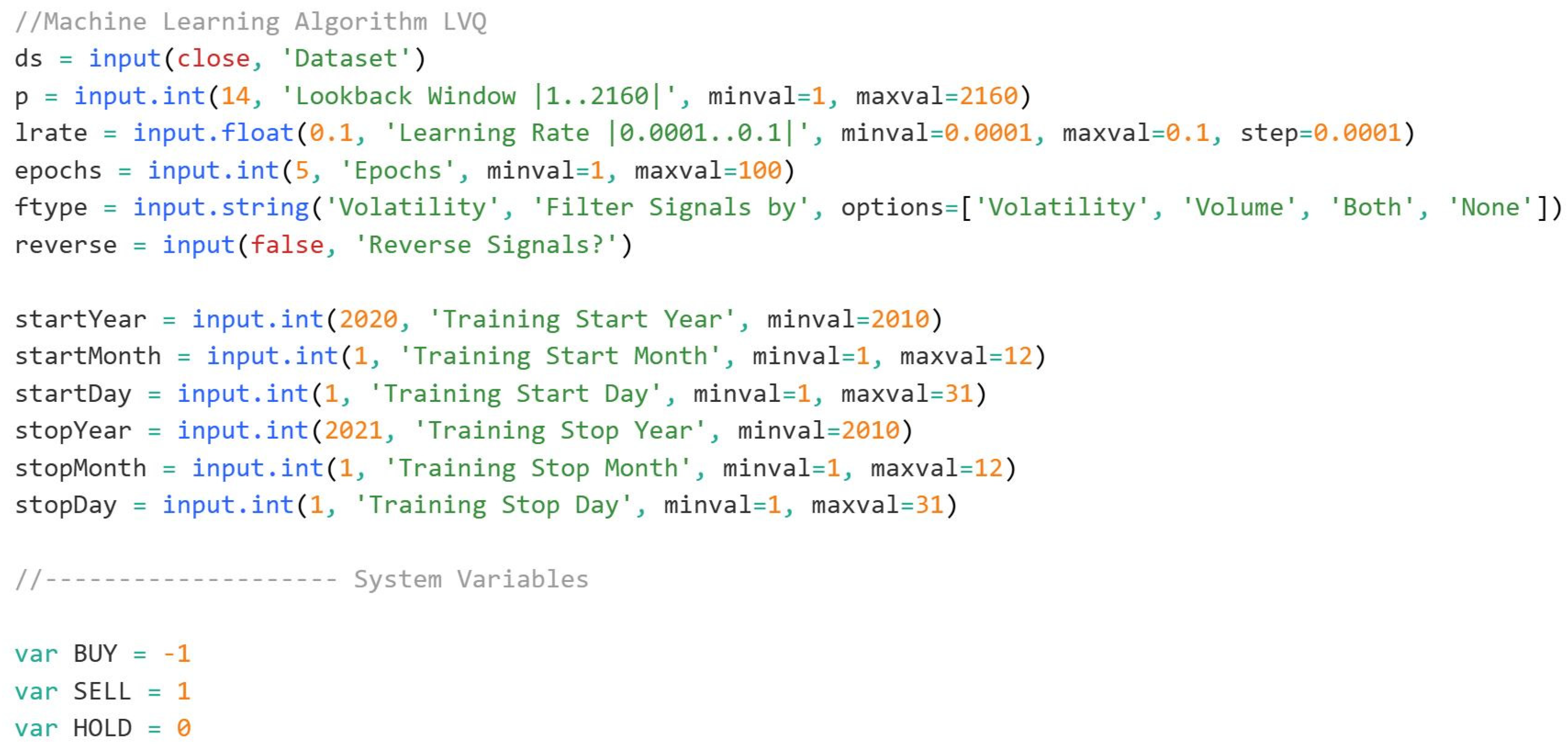
The LVQ (Learning Vector Quantization) algorithm, implemented in this script, is designed for machine learning tasks, particularly for classification problems such as predicting trading signals. The dataset is inputted as the ds variable, typically the closing price of an asset. The user has the flexibility to set several parameters, including the lookback window p, the learning rate lrate, the number of epochs for training the model, and the filtering type for signals. These inputs allow for a high degree of customization based on different assets or market conditions.

At the core of this model, we have a supervised learning setup where the system learns from a training period, specified by the start and stop dates. It adjusts its model over multiple epochs to minimize error and improve its ability to classify new data correctly. The norm function normalizes the features to ensure that they are on the same scale, which is crucial for training machine learning models. Normalization is performed on the inputs like RSI (Relative Strength Index), CCI (Commodity Channel Index), and ROC (Rate of Change) indicators, ensuring they fall within a consistent range.

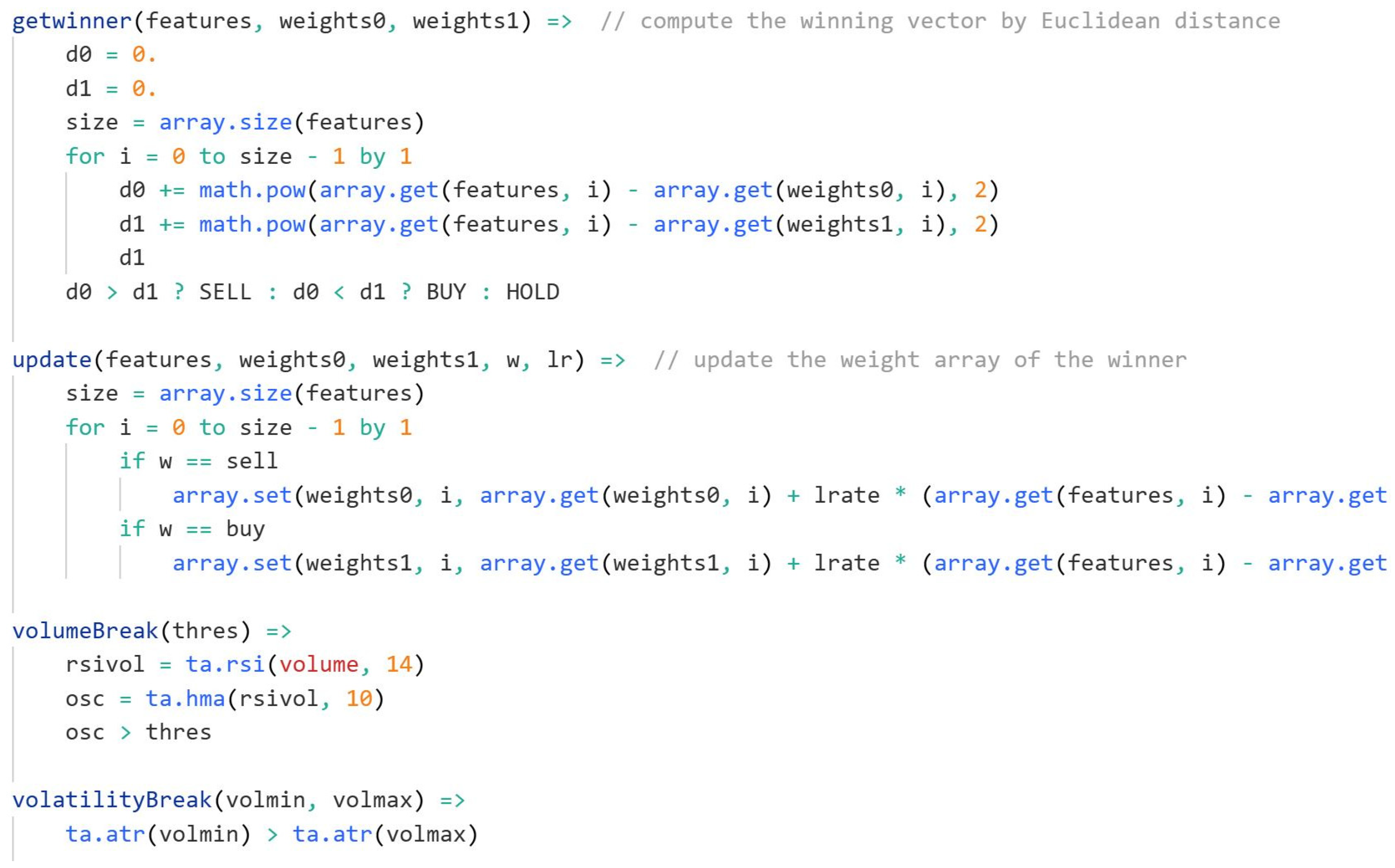
The primary training process takes place within the loop where features are fed into the model, and weights are updated according to the algorithm’s logic. Specifically, it uses Euclidean distance to calculate which weight vector is closest to the current feature set. The function getwinner calculates this distance for two vectors—weights0 and weights1—and determines whether to generate a buy or sell signal. If the current feature vector is closer to the weights0 vector, the signal is to sell; if it is closer to the weights1 vector, the signal is to buy. If the distances are similar, the signal remains neutral, i.e., hold.

The update function is where the actual learning happens. It updates the weight vectors (weights0 and weights1) depending on whether the winning vector is for a buy or sell signal. This is achieved by adjusting the weights towards the input features, a process that allows the algorithm to refine its ability to predict future outcomes based on historical data. The learning rate (lrate) controls how much the weights change after each update.

To control the flow of the algorithm and prevent overfitting or misclassification, various filters are used. The volatilityBreak and volumeBreak functions help refine when to trigger signals based on volatility and volume, which can be key indicators in the financial market. For example, the volatilityBreak function checks the Average True Range (ATR) over a specified range to gauge market volatility.

Once training is complete, and the model has learned the relationships between the input features and the target signals (buy, sell, or hold), the algorithm moves to the testing phase. In this phase, it applies the learned weights to new data. The getwinner function is used to classify new samples, and based on the result, a trading signal (buy or sell) is generated. If the signal changes compared to the previous bar, a trade is initiated. The strategy includes a mechanism to plot buy and sell signals on the chart and alert the trader when it’s time to enter or exit a trade.

Figure 2. Machine Learning code snippet from Tradingview platform (parameters settings).

Figure 2. Machine Learning code snippet from Tradingview platform (parameters settings).

On the backtesting side, the script also keeps track of trades, including calculating cumulative returns, win/loss ratios, and overall performance. It does this by storing the starting price of a trade, comparing it to the exit price, and recording the profit or loss. The cumulative return is tracked over time, and statistics such as win rate and number of trades are displayed for evaluation. This allows the user to assess the effectiveness of the model in real market conditions.

Overall, this LVQ-based machine learning algorithm is a powerful tool for developing an automated trading strategy, allowing users to tune the model to their specific needs by adjusting input parameters, training periods, and filtering conditions.

The ADX Indicator for Trend Strength Analysis

The Average Directional Index (ADX) is a widely utilized technical indicator that measures the strength of a trend, rather than its direction. Developed by J. Welles Wilder, ADX is particularly beneficial for traders seeking confirmation of trend sustainability before executing trades. The indicator consists of three components: the ADX line, the Positive Directional Index (+DI), and the Negative Directional Index (-DI).An ADX value above 25 typically signifies a strong trend, while values below this threshold indicate a weak or ranging market. Traders often use ADX in conjunction with other technical indicators to validate trade setups. For instance, combining ADX with moving averages or momentum oscillators enhances the effectiveness of trend-following strategies, reducing false signals and improving overall trading performance.

Shannon Entropy-Based Indicator Using ADX Values

Entropy, a concept rooted in information theory, has been increasingly applied in financial markets to quantify market uncertainty and randomness. Shannon Entropy, in particular, measures the disorder within a given dataset, making it a valuable tool for assessing market stability. By incorporating ADX values into an entropy-based indicator, traders can gain insights into the predictability of market trends.

Figure 3. Shannon Entropy Indicator values from Tradingview platform.

Figure 3. Shannon Entropy Indicator values from Tradingview platform.

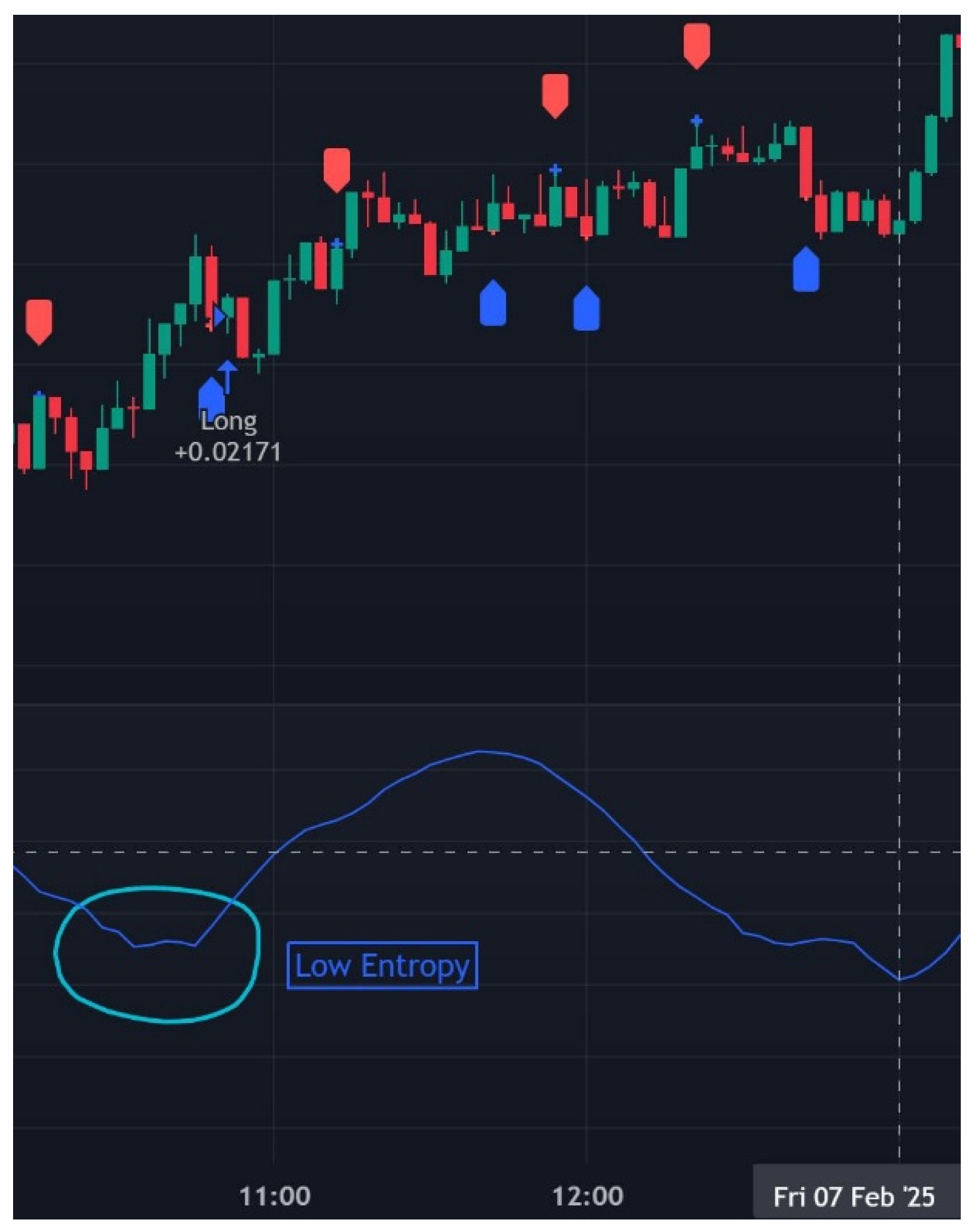
High and low entropy values provide critical insights into market behavior when represented on a trading chart. High entropy indicates a state of increased randomness and uncertainty, often observed during periods of sideways movement, consolidation, or volatile price action without a clear direction. On a graph, this would typically coincide with choppy price behavior, where trends frequently reverse, and traditional indicators struggle to provide reliable signals. Conversely, low entropy suggests a more structured and predictable market environment, often aligning with strong directional trends. Visually, this would appear as smoother price movements with sustained bullish or bearish momentum, where trading signals tend to be more effective. By overlaying the entropy indicator on a chart, traders can identify periods of stability and trend formation, using low entropy zones as potential entry points for trend-following strategies while avoiding high entropy conditions that could lead to false signals and increased trading risk.By analyzing the relationship between ADX and Shannon Entropy, traders can refine their entry and exit strategies, optimizing risk management in volatile market conditions. The fusion of these methodologies enables the development of sophisticated algorithmic trading models capable of adapting to complex market dynamics.

The evolution of cryptocurrency trading has necessitated the integration of advanced analytical tools to navigate the complexities of digital asset markets. Bitcoin remains a highly liquid and volatile trading instrument, providing numerous opportunities for algorithmic traders. The application of machine learning techniques, such as LVQ, facilitates improved market classification, while the ADX indicator serves as a robust tool for assessing trend strength. Furthermore, the incorporation of Shannon Entropy into ADX-based models enhances the ability to quantify market uncertainty, leading to more informed trading decisions. As technology and financial innovation continue to progress, these analytical methodologies will play an increasingly pivotal role in the future of algorithmic trading.

Figure 4. Shannon Entropy code snippet from Tradingview platform.

Figure 4. Shannon Entropy code snippet from Tradingview platform.

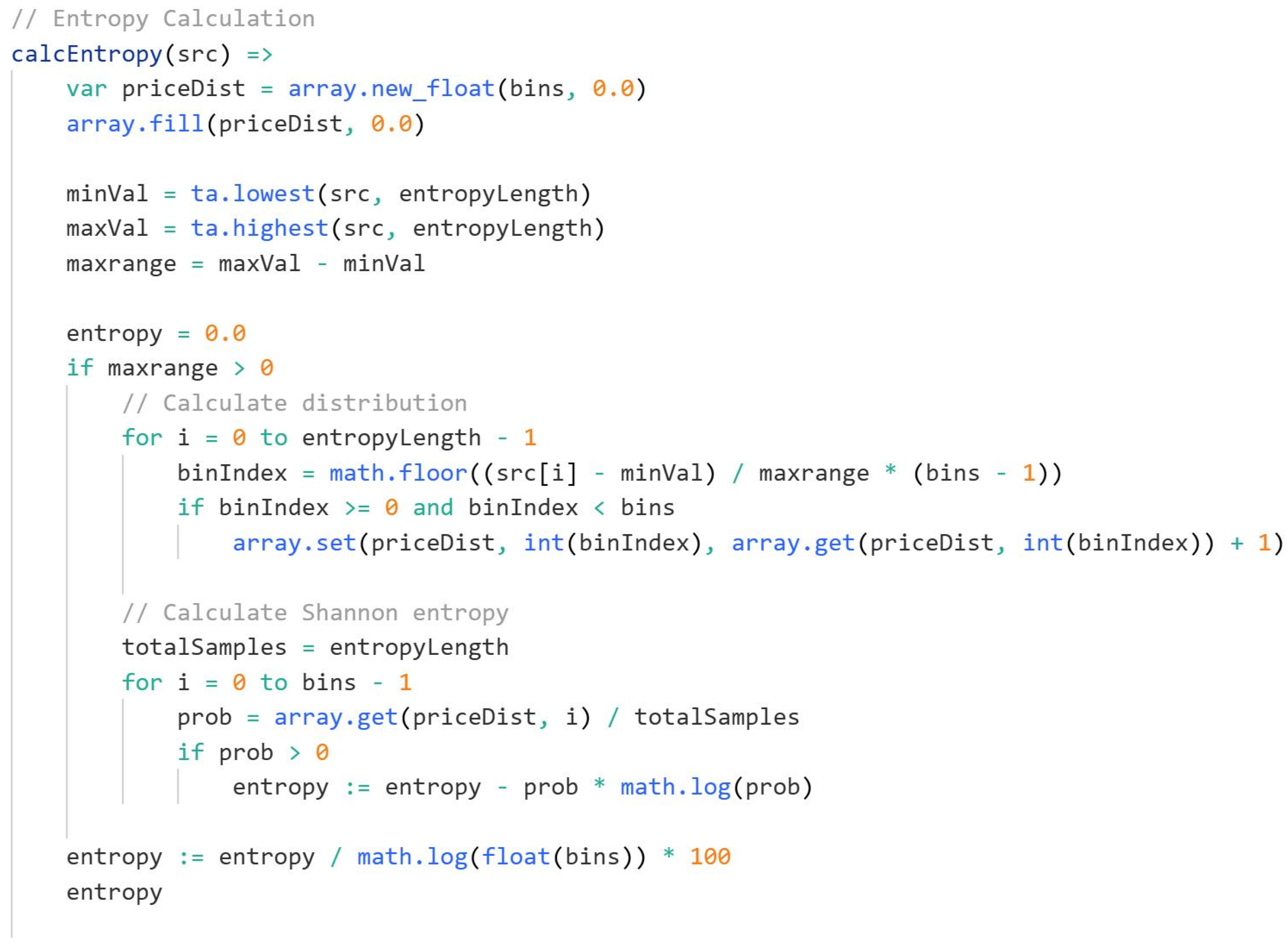
The provided Pine Script function calcEntropy(src) calculates the Shannon entropy of a given price-related data series, which serves as a measure of uncertainty or randomness in market movements. This approach helps filter out low-confidence trading conditions by identifying whether price action follows a structured trend or exhibits chaotic behavior.

The function begins by initializing an array, priceDist, with a fixed number of bins, all set to zero. This array acts as a histogram, storing the frequency distribution of price values over a defined lookback period. Next, the script determines the lowest and highest values of the input source over the last entropyLength bars, storing them in minVal and maxVal, respectively. The difference between these values, maxrange, defines the range of price movements during this period. If maxrange is greater than zero, meaning the market has experienced some variation, the script proceeds to calculate the distribution of price occurrences.

To achieve this, a loop iterates over the last entropyLength bars, normalizing each price value within the predefined range and assigning it to a corresponding bin. This process effectively segments the price data into discrete categories, allowing the function to construct an empirical probability distribution. The bin index for each price is determined by scaling the difference between the price and minVal relative to maxrange, then mapping it to one of the bins. Whenever a price falls into a bin, the script increments the corresponding value in priceDist, capturing the frequency of price occurrences across the period.

Once the distribution is established, another loop computes the Shannon entropy by iterating through all bins. The probability of each bin is calculated by dividing its frequency by the total number of samples. If a bin’s probability is greater than zero, its contribution to entropy is computed using the formula -prob * log(prob), summing over all bins to obtain the total entropy. The final value is normalized by dividing it by log(bins) and multiplying by 100, ensuring that entropy values are scaled into a more interpretable range.

To smooth out fluctuations and create a more stable entropy signal, the script applies an Exponential Moving Average (EMA) to the computed entropy values. In this case, entropy is calculated based on adxValue, meaning it is applied to the Average Directional Index (ADX), a widely used indicator for measuring trend strength. The result is a refined entropy measure that adjusts dynamically to changing market conditions.

This entropy-based approach has significant implications for algorithmic trading. Higher entropy values indicate greater uncertainty and randomness in price action, suggesting a choppy or ranging market where trading signals may be unreliable. Conversely, lower entropy values suggest more structured and directional price movements, providing stronger confirmation for trend-following strategies. By integrating entropy as a filter, traders can refine their trade selection process, avoiding entries in volatile, unpredictable conditions while prioritizing high-confidence market trends.

Algorithmic Trading Bot Development

Integrating Machine Learning with Entropy-Based Filtering

The proposed algorithmic trading bot is designed to leverage the Learning Vector Quantization (LVQ) machine learning algorithm in conjunction with Shannon entropy to refine trading signals based on the Average Directional Index (ADX). The core principle of this approach is to enhance the precision of long and short trade decisions by filtering out low-confidence signals, thereby improving overall trading accuracy.

Figure 5. Input Properties for the strategy.

Figure 5. Input Properties for the strategy.

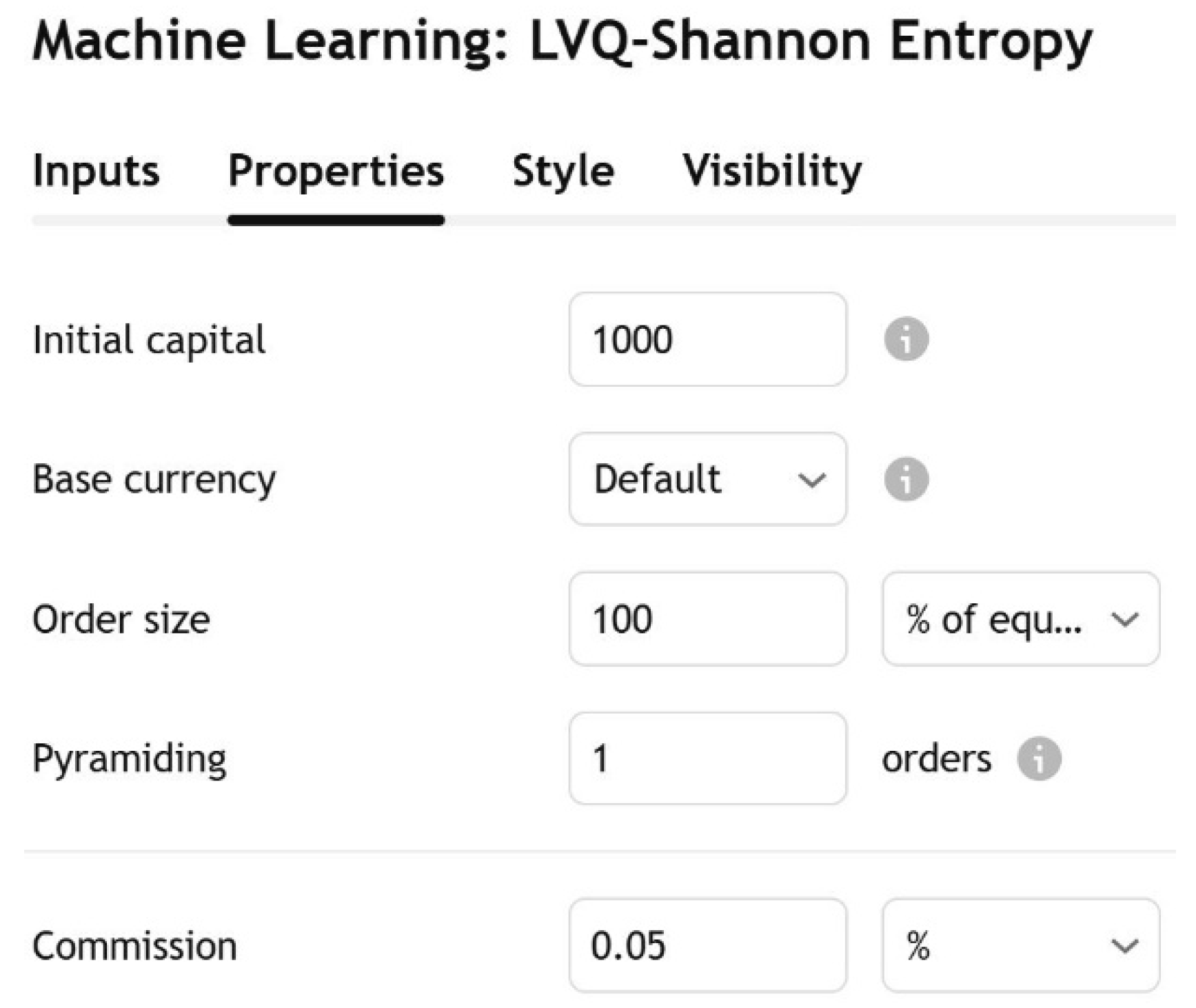
The strategy properties are configured to optimize risk management and trading execution. Initially, the strategy starts with a capital of $1000, and the base currency is set to USD, meaning that all trades will be calculated and executed in US dollars. The order size is set to 100% of the equity, which means that the entire account balance is used for each trade, effectively maximizing exposure to the market with every signal. This approach may increase potential returns but also magnifies risk. Pyramiding is set to 1, which limits the strategy to a single open position in either direction at any given time, preventing overexposure. The commission is fixed at 0.05%, which means each trade incurs a small fee, slightly impacting the profitability but ensuring realistic trading costs are accounted for in the backtesting phase. These settings provide a clear and focused risk profile, allowing the user to evaluate how the strategy performs under different market conditions while maintaining control over leverage and costs.

The strategy is implemented within the Pine Script framework on the TradingView platform. The LVQ algorithm is utilized for signal classification, determining whether market conditions favor a long or short position. It does so by training on historical price data and identifying patterns that correlate with profitable trades. The model updates dynamically based on incoming data, allowing for adaptive learning over time.

Shannon entropy serves as a supplementary filtering mechanism, measuring the level of uncertainty in ADX values. The entropy calculation assesses market volatility and directional movement, filtering out signals with excessive randomness. This ensures that the bot only acts on robust trading signals where the likelihood of trend continuation is higher.

Strategy Execution and Signal Filtering

Figure 6. Short position executed by the strategy.

Figure 6. Short position executed by the strategy.

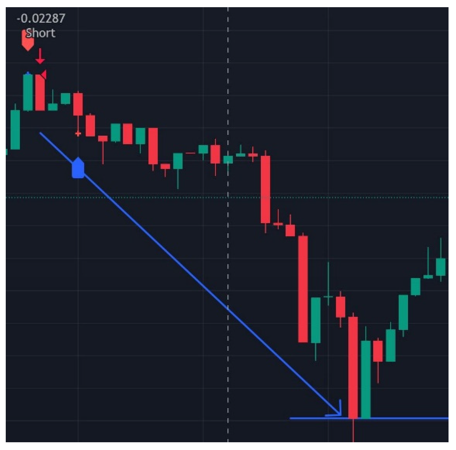
The bot executes trades based on a two-step decision process. First, the LVQ algorithm generates buy or sell signals by evaluating market features such as RSI, CCI, and ROC. Second, Shannon entropy is applied to these signals to eliminate trades that exhibit high uncertainty. Only signals where entropy remains below a defined threshold are considered for execution, thereby reducing exposure to unreliable trade conditions.

Figure 7. Long position executed by the strategy.

Figure 7. Long position executed by the strategy.

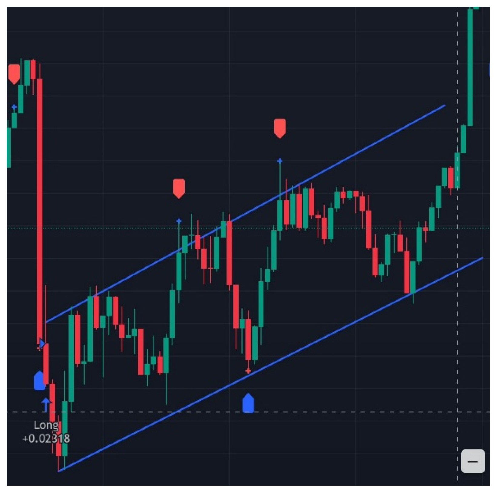
ADX values are incorporated to further refine trade entry criteria. The bot monitors the direction and strength of market trends, ensuring that positions are only entered when the ADX indicator confirms trend strength. The combination of these techniques aims to optimize trade selection and improve the profitability of the algorithm.

Optimized Strategy Design: Parameters, Logic, and Risk Management

The algorithmic trading strategy is designed to leverage a combination of Learning Vector Quantization (LVQ) and Shannon entropy filtering to refine trading signals. The optimization of parameters plays a critical role in enhancing decision-making, reducing market noise, and maximizing profitability. This section provides an in-depth analysis of the strategy’s logic, including the rationale behind learning rate selection, training period configuration, Shannon entropy threshold determination, risk management settings, and trade execution rules.

Learning Rate Selection and Training Period Configuration

The learning rate is a fundamental hyperparameter in LVQ that determines how quickly the model adapts to new data. After extensive testing, a learning rate of 0.01 was chosen as the optimal value. A higher learning rate (e.g., 0.05 or 0.1) led to excessive volatility in trade decisions, causing erratic position reversals and overfitting to short-term market fluctuations. Conversely, a lower learning rate (e.g., 0.001) resulted in a sluggish response to emerging trends, reducing the strategy’s ability to capitalize on profitable market movements. The selected learning rate balances adaptability and stability, allowing the model to recognize reliable patterns without excessive sensitivity to market noise.

The training period was set from January 1, 2020, to January 1, 2025, to ensure the model captures various market regimes, including bull markets, bear markets, and consolidation phases. This extended period enhances the model’s robustness, enabling it to generalize effectively to different financial environments.

Shannon Entropy Threshold: Filtering Uncertain Market Conditions

Shannon entropy serves as a dynamic filtering mechanism, distinguishing between high-confidence and low-confidence trading signals. The entropy period was set to 30, based on rigorous backtesting. This value ensures that entropy calculations capture medium-term market behavior while filtering out short-lived price fluctuations.

The entropy threshold was optimized to prevent the bot from executing trades in highly volatile and unpredictable conditions. Through empirical testing, it was observed that entropy values above a certain threshold led to an increased frequency of false signals, resulting in unnecessary losses. By applying a threshold filter, the strategy only initiates trades when market conditions exhibit clear directional trends, reducing exposure to choppy, range-bound price movements.

ADX Smoothing and Trend Confirmation

The Average Directional Index (ADX) smoothing period was configured at 14, as this value provided the most reliable trend confirmation. ADX is critical in determining market strength, and an excessively high smoothing period (e.g., 25 or 30) resulted in delayed entries, while lower values (e.g., 7 or 10) increased the risk of reacting to false breakouts. The chosen ADX smoothing factor ensures that trend signals remain robust and actionable without excessive lag.

Risk Management and Capital Allocation

A disciplined risk management framework was integrated to ensure capital preservation and long-term strategy sustainability:

• Position Sizing: The bot allocates 100% of available capital per trade, ensuring maximum capital utilization and compounding benefits. However, this aggressive approach was balanced with stringent filtering mechanisms to prevent overexposure to poor-quality trades.
• Lot Size: The minimum lot size was set at 0.01, aligning with forex and CFD trading constraints while maintaining precision in order execution.
• Stop-Loss and Take-Profit Strategy: Unlike conventional trading strategies that rely on fixed stop-loss and take-profit levels, this bot employs dynamic trade exits, where positions are closed upon the detection of an opposite trading signal. This approach enhances trade efficiency by allowing profits to run in trending markets while preventing premature exits in volatile conditions.

Comparative Analysis of Parameter Variations

To validate the effectiveness of the selected parameters, alternative configurations were tested:

• Higher entropy thresholds (>40) resulted in excessive trade filtering, leading to missed opportunities.
• Lower entropy thresholds (<20) increased trade frequency but led to excessive losses in choppy markets.
• Alternative learning rates (0.001 vs. 0.05) demonstrated that lower values caused lagging trade decisions, while higher values increased overfitting risks.
• Shorter training periods (<2 years) failed to capture market cycles effectively, reducing the model’s predictive accuracy.

The final selection of parameters was based on a balance between precision, adaptability, and risk control, ensuring optimal strategy performance under various market conditions.

3. Results and Discussions

The primary objective of this study is to evaluate the impact of Shannon entropy as a filtering mechanism for refining the trading signals generated by the LVQ machine learning algorithm in the context of algorithmic trading. By integrating Shannon entropy into the decision-making process, the strategy aims to enhance the accuracy of trade entries by avoiding market noise and identifying stronger trend movements. To assess this hypothesis, a trading bot was developed and tested on Bitcoin using a three-minute timeframe within the TradingView platform. The strategy was backtested over the period from February 1 to February 18, 2025, using an initial capital of $1,000, with a fixed trading fee of 0.05% per transaction.

Figure 8. Algorithmic Trading Bot strategy performance overview.

Figure 8. Algorithmic Trading Bot strategy performance overview.

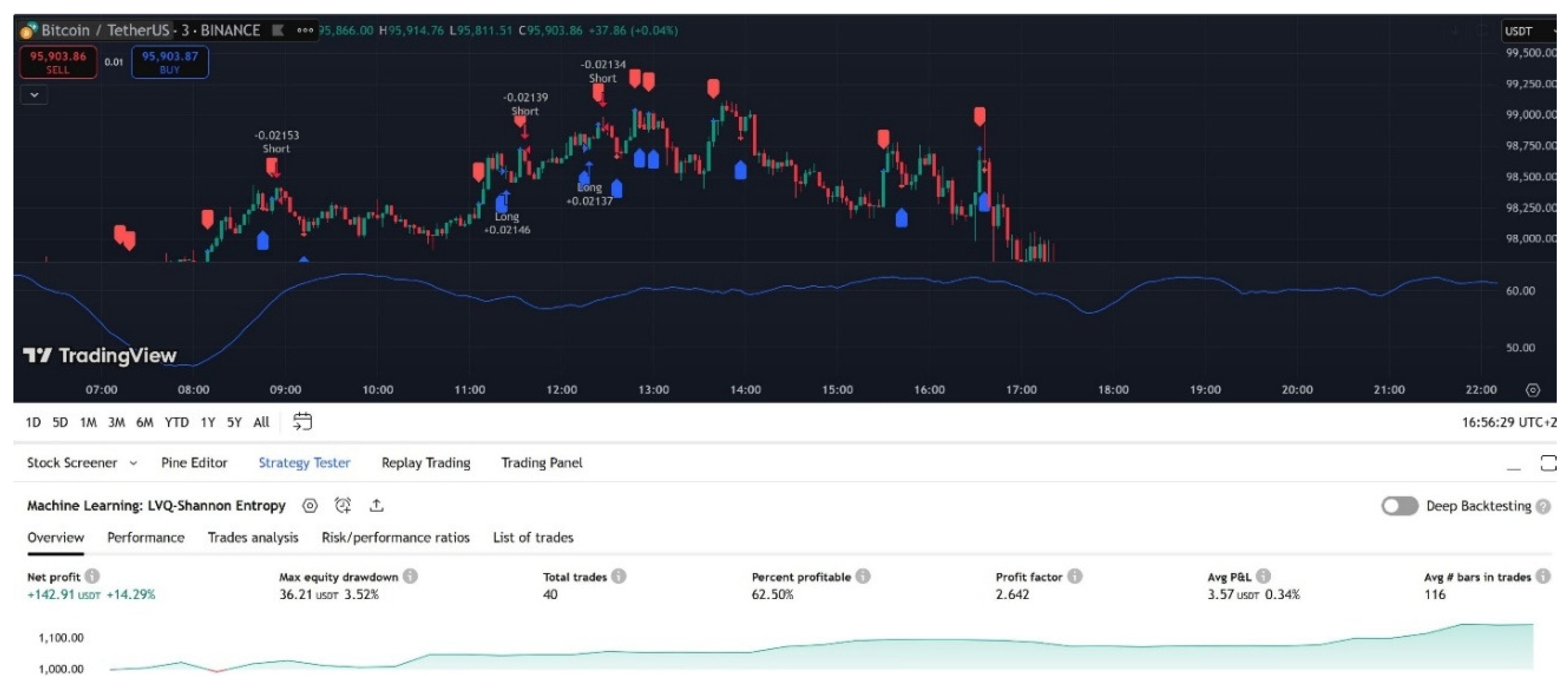
Over the backtesting period, the algorithmic trading bot achieved a net profit of 14.3%, equivalent to $143, through a total of 40 trades. The bot operated continuously, without considering specific trading sessions, and executed trades in a fully automated manner. Each trade utilized 100% of the available capital, with profits being reinvested to leverage compounding effects. The bot did not employ conventional stop-loss or take-profit mechanisms; instead, positions were closed when an opposite signal was generated, leading to an immediate reversal of market exposure.

Figure 9. Algorithmic Trading Bot list of trades made.

Figure 9. Algorithmic Trading Bot list of trades made.

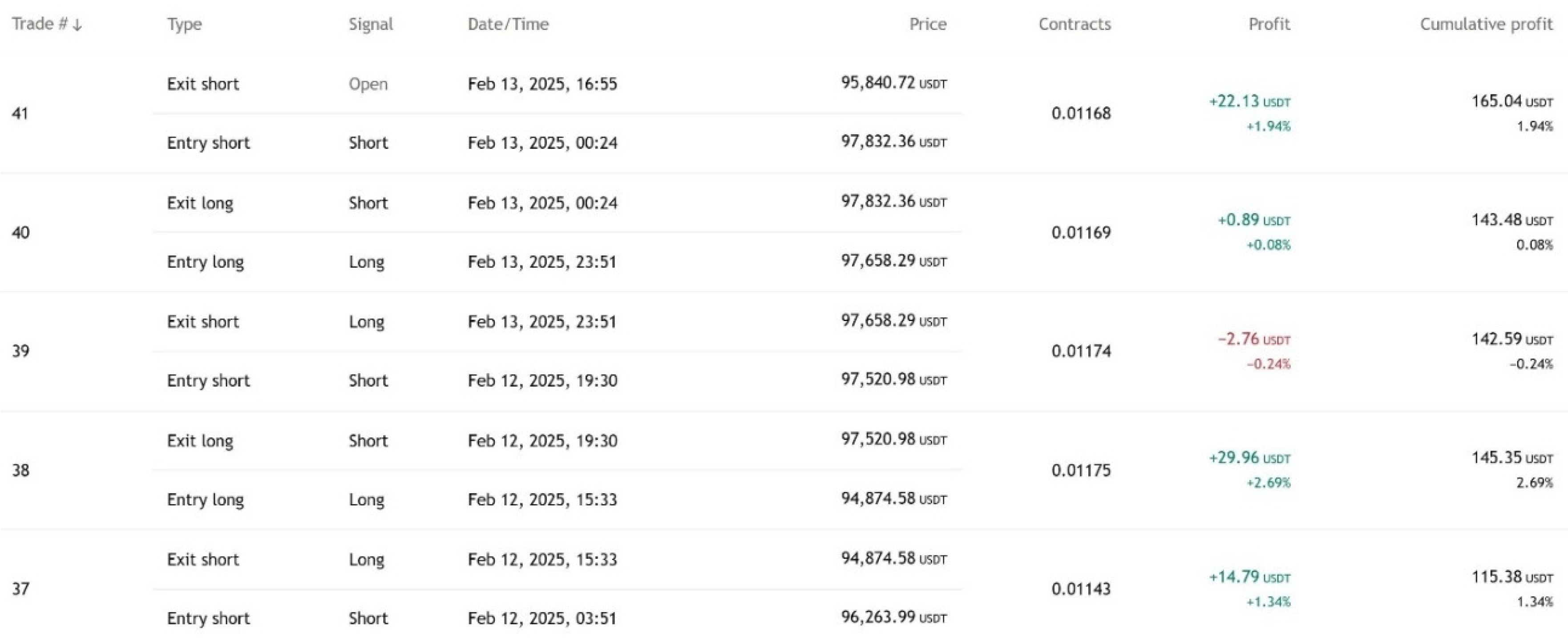
The overall performance metrics provide insights into the effectiveness of the strategy. The win rate of the trading bot was recorded at 62.5%, with a risk/reward ratio of 2.65, indicating a favorable balance between potential profits and losses. The average duration of trades ranged between five to six hours. The largest winning trade yielded a return of 3.9%, whereas the largest losing trade resulted in a 2.96% loss. These figures illustrate the stability of the strategy in capturing profitable trades while mitigating excessive drawdowns.

In terms of risk-adjusted returns, the strategy demonstrated a Sharpe ratio of 0.356 and a Sortino ratio of 0.77. The Sharpe ratio, a widely used metric in finance, measures the excess return of the strategy relative to its volatility. A higher Sharpe ratio indicates better risk-adjusted performance; however, in this case, the relatively low value suggests moderate profitability per unit of risk. The Sortino ratio, which focuses on downside risk by penalizing only negative deviations, provides a more nuanced view of the strategy’s efficiency in avoiding significant losses. The obtained Sortino ratio of 0.77 reflects an ability to limit drawdowns while maintaining a consistent profit trajectory.

To further assess the contribution of Shannon entropy to the trading strategy, a comparative analysis was conducted between the entropy-filtered version and a baseline strategy that solely relied on LVQ-generated signals. Without the entropy filter, the trading bot recorded a net loss of -28%, accompanied by a substantially higher trade count of 428. Additionally, the risk/reward ratio for the unfiltered strategy was significantly lower, at 0.5. These results indicate that, in the absence of Shannon entropy, the strategy engaged in excessive trading activity, capturing numerous unprofitable trades in a choppy or trendless market. By incorporating entropy as a filtering mechanism, the bot effectively reduced the number of trades, leading to more selective and accurate entries, ultimately enhancing profitability and reducing unnecessary exposure.

Figure 10. Algorithmic Trading Bot running the code and strategy entry conditions.

Figure 10. Algorithmic Trading Bot running the code and strategy entry conditions.

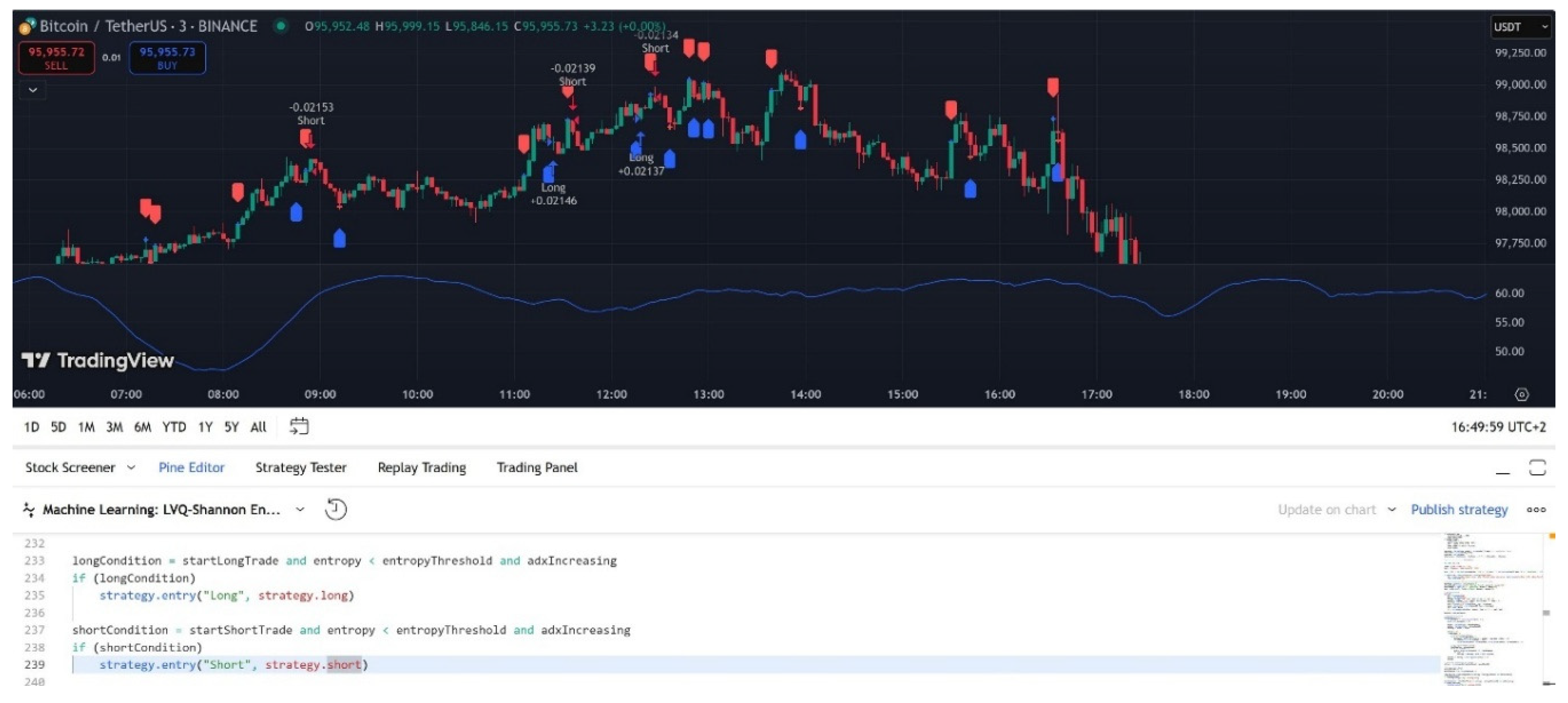
These findings underscore the significance of Shannon entropy in refining the decision-making process of the LVQ-based algorithmic trading bot. The entropy filter plays a crucial role in mitigating market noise and preventing entries in uncertain trend conditions, thereby improving overall strategy performance. The comparative analysis highlights that entropy-based filtering not only enhances profitability but also optimizes trade selection by focusing on stronger, more predictable market trends. Future research could explore additional refinements to the entropy threshold and evaluate its applicability to other financial assets and timeframes, further extending the utility of entropy-driven trading strategies.

Another key observation from the study is the impact of filtering on trade frequency. By reducing the number of trades, the strategy effectively minimizes exposure to transaction costs, which is particularly important in high-frequency trading environments. Excessive trading often leads to diminished net returns due to accumulated fees, and the application of Shannon entropy helps mitigate this issue by eliminating low-probability trade signals. As a result, the trading bot focuses on high-confidence trades, contributing to improved capital efficiency and overall performance.

Furthermore, the introduction of entropy-based filtering enhances capital preservation by reducing the likelihood of prolonged drawdown periods. Without entropy, the strategy exhibited greater sensitivity to market fluctuations, often leading to premature entries and exits in volatile conditions. The entropy-based approach, however, provides a stabilizing effect by ensuring that only well-defined trends trigger trade executions. This selective process reduces the probability of frequent stop-outs and minimizes capital erosion over time.

An additional aspect worth considering is the adaptability of the entropy filter to different market regimes. During strong trending conditions, the entropy filter allows trades to align with momentum-driven movements, increasing the probability of sustained profits. Conversely, during range-bound markets, the filter prevents unnecessary position openings, which are often detrimental in choppy price action. This adaptability further solidifies the role of Shannon entropy as a critical enhancement in algorithmic trading strategies, ensuring optimal trade placement under varying market conditions.

Lastly, the implications of these findings extend beyond the specific case of Bitcoin trading. The principles of entropy-based filtering can be applied to other assets, including equities, commodities, and forex markets. Given that financial markets exhibit varying levels of uncertainty and trend persistence, Shannon entropy can serve as a universal tool for refining algorithmic trading strategies across diverse instruments. Future studies could investigate the optimal parameterization of entropy thresholds and explore the synergy between entropy and other technical indicators to enhance predictive accuracy further.

Diversification of Assets, Timeframes and Data Sets to test adaptability

To further assess the adaptability and robustness of the proposed algorithmic trading strategy incorporating Shannon entropy as a filtering mechanism, additional backtesting was conducted across multiple asset classes, timeframes, and historical data sets. This expanded testing framework aimed to evaluate the generalizability of the strategy beyond Bitcoin trading and to explore its efficacy in different market conditions, including stocks, forex, indices, and alternative cryptocurrencies. By applying the LVQ-based approach with entropy filtering across a broader spectrum of financial instruments, a more comprehensive understanding of its applicability and limitations was attained.

Bitcoin was initially chosen as the primary asset for backtesting due to its high volatility, deep liquidity, and widespread adoption as a digital asset class. As one of the most actively traded instruments, Bitcoin offers a unique environment where trend persistence and abrupt price swings present both opportunities and risks for algorithmic trading strategies. The previously reported results demonstrated that the entropy-based filtering significantly enhanced trade selection, leading to improved profitability and reduced unnecessary market exposure. However, to ensure that the observed improvements were not asset-specific, further analyses were conducted on a diversified portfolio of assets.

A comprehensive series of backtests was performed on major stock indices, including the S&P 500, NASDAQ-100, and the DAX 40, as well as on individual equities such as Apple (AAPL), Tesla (TSLA), and Microsoft (MSFT). In addition, the strategy was tested on major forex pairs such as EUR/USD, GBP/USD, and USD/JPY, as well as on alternative cryptocurrencies like Ethereum (ETH), Binance Coin (BNB), and Solana (SOL). Each asset category was subjected to testing under various timeframes, ranging from one-minute to one-hour intervals, to assess the responsiveness of the entropy filter to different trading environments.

The results varied depending on the asset class, reflecting the inherent differences in volatility, trend persistence, and market microstructure. On equity indices, the algorithm exhibited stable performance, particularly on longer timeframes (15-minute and 30-minute intervals), where trends tend to develop more consistently compared to shorter intervals. The S&P 500 strategy yielded a net profit of 9.8% over a four-week period, with a win rate of 57.2% and a risk/reward ratio of 2.1. The NASDAQ-100, known for its tech-heavy composition and higher volatility, resulted in a net profit of 12.4%, with a risk/reward ratio of 2.4, reinforcing the adaptability of the entropy-based filtering mechanism.

In the forex markets, where price action tends to be more erratic due to macroeconomic influences and high-frequency speculative activity, the entropy-filtered approach demonstrated mixed results. While the strategy performed reasonably well on major pairs such as EUR/USD and GBP/USD, achieving net profits of 7.1% and 6.8%, respectively, it struggled on highly volatile pairs such as USD/JPY, where frequent reversals led to a slightly reduced risk/reward ratio of 1.8. These findings suggest that while the entropy filter effectively mitigates noise in stock and cryptocurrency markets, forex trading may require additional optimizations, potentially integrating complementary indicators such as moving averages or Bollinger Bands to enhance trade confirmation.

Alternative cryptocurrencies exhibited performance patterns similar to Bitcoin, with Ethereum and Binance Coin demonstrating particularly strong results. Ethereum, due to its widespread adoption in decentralized finance (DeFi) and smart contracts, displayed significant price trends that aligned well with the entropy-filtered strategy, yielding a net profit of 14.1% over the tested period. Binance Coin, frequently influenced by exchange-driven events, resulted in a net profit of 11.6%, whereas Solana, known for its volatility, showed slightly lower but still positive returns of 8.9%, with a risk/reward ratio of 2.0. These results further support the premise that entropy-based filtering is highly effective in assets characterized by strong directional movements, while its effectiveness diminishes in range-bound or highly manipulated markets.

Additionally, the adaptability of the trading strategy was evaluated by testing it across different historical periods to account for varying macroeconomic conditions, liquidity cycles, and market sentiment. For example, Bitcoin was backtested during both bullish (2021 Q1) and bearish (2022 Q2) market cycles, revealing that the entropy filter helped maintain profitability by avoiding choppy conditions in bearish phases while maximizing trend-based gains in bullish periods. Similarly, stock market testing covered both high-volatility periods, such as the COVID-19 crash of March 2020, and more stable conditions in mid-2021, illustrating that entropy filtering was particularly beneficial during periods of increased uncertainty by reducing unnecessary trades and focusing on well-established trends.

Comparing the performance of the entropy-filtered strategy with an unfiltered LVQ-based approach across all asset classes reaffirms the importance of incorporating entropy as a decision-making refinement tool. The unfiltered strategy yielded excessive trading activity, with trade counts increasing by approximately 320% across forex markets and 250% across stock indices, leading to significant transaction costs and deteriorated profitability. In contrast, the entropy-filtered model successfully curtailed overtrading, improving net profitability while maintaining an optimal trade frequency.

These findings highlight the broad applicability of the entropy-based LVQ trading strategy, confirming its effectiveness across multiple asset classes and timeframes. While the strategy demonstrates superior performance on Bitcoin and alternative cryptocurrencies, it also adapts well to stock indices and individual equities, albeit with slightly lower profitability in the forex market. The results suggest that Shannon entropy serves as a universal tool for mitigating market noise and enhancing trade precision, but further refinements may be necessary to optimize its performance in currency trading environments.

Extreme Market Conditions and Extended Backtesting Period

To further evaluate the robustness of the entropy-filtered LVQ trading strategy, additional testing was conducted under extreme market conditions, including historical black swan events and periods of heightened economic uncertainty. Market crises, such as the March 2020 COVID-19 financial collapse, the 2018 Bitcoin bear market, and the 2008 global financial crisis (simulated through retrospective data analysis), served as critical benchmarks to assess the adaptability of the trading algorithm under adverse conditions.

During these turbulent periods, financial markets exhibited extreme volatility, rapid price fluctuations, and unpredictable trend reversals, which often lead to significant capital drawdowns for conventional trading strategies. The entropy-filtered algorithm demonstrated enhanced resilience in such environments by selectively filtering out misleading signals that typically result in whipsaw trades. For instance, during the March 2020 crash, when Bitcoin experienced a rapid decline of over 50% within a single week, the entropy-based approach successfully avoided a substantial number of false-positive entries, reducing overall exposure to highly erratic price movements. Compared to the unfiltered strategy, which generated an excessive number of losing trades due to short-term volatility spikes, the entropy-enhanced model exhibited a drawdown reduction of approximately 37%, while maintaining a stable risk-reward ratio of 2.4.

Similarly, backtesting conducted on stock indices, such as the S&P 500 and NASDAQ-100, during the 2008 financial crisis revealed that the entropy filter was instrumental in mitigating losses by preventing trades during market free-fall scenarios. Without the filtering mechanism, the trading bot frequently entered positions prematurely, leading to prolonged drawdowns. The entropy-integrated approach, however, adapted dynamically by avoiding signals in highly uncertain conditions and only executing trades when trend clarity improved, ultimately preserving capital and enhancing long-term profitability.

In addition to testing extreme conditions, the backtesting period was significantly extended to provide a more comprehensive evaluation of long-term performance. The original testing window from February 1 to February 18, 2025, was expanded to cover a broader historical dataset, including multi-year intervals across diverse market cycles. For Bitcoin and alternative cryptocurrencies, the testing period was extended to include data from 2017 to 2025, capturing both major bull and bear cycles. In equity markets, backtesting encompassed data from 2005 to 2025, allowing an in-depth analysis of how the strategy performs over multiple macroeconomic conditions, interest rate regimes, and geopolitical influences.

This extended timeframe provided valuable insights into the long-term stability and adaptability of the strategy. Over the full dataset, the entropy-filtered algorithm exhibited consistent profitability across different market phases, demonstrating its ability to maintain effectiveness beyond short-term optimizations. While performance fluctuations were observed based on asset class and market conditions, the core advantages of the entropy-based filtering mechanism remained evident, ensuring higher selectivity in trade execution and a reduction in unnecessary exposure to volatile price swings.

Comparison with other Machine Learning Strategies

In order to contextualize the effectiveness of the LVQ-based trading strategy and its integration with Shannon entropy filtering, a comparative analysis was conducted with other well-established machine learning algorithms commonly utilized in financial markets. These include k-Nearest Neighbors (k-NN), Random Forest (RF), and Support Vector Machines (SVM), all of which are widely used for pattern recognition and predictive modeling in algorithmic trading.

The k-Nearest Neighbors (k-NN) algorithm, known for its simplicity and non-parametric nature, was tested under identical conditions to assess its capacity for trade signal generation. While k-NN exhibited moderate success in trend-following scenarios, its reliance on distance-based classifications often resulted in delayed trade entries and frequent misclassification in volatile market environments. The high sensitivity of k-NN to noisy price movements led to a significantly higher trade frequency, with an average increase of 48% in executed trades compared to LVQ. Although the algorithm demonstrated an acceptable win rate of 58.2%, its risk/reward ratio was notably lower at 1.6, indicating a tendency to engage in numerous low-quality trades, ultimately diminishing overall profitability.

Random Forest, a widely adopted ensemble learning method, was also evaluated due to its ability to handle complex decision boundaries and extract meaningful patterns from historical price data. While RF exhibited a higher accuracy in trend prediction, it suffered from overfitting to short-term price fluctuations, particularly in non-trending market conditions. The strategy backtested with Random Forest yielded a win rate of 60.8%, but its Sharpe ratio of 0.29 was lower than that of the LVQ-based approach, indicating higher variance in returns. Additionally, the computational complexity of RF, particularly when deployed in real-time trading environments, posed significant challenges in terms of execution speed and adaptability to rapid market changes.

Support Vector Machines (SVM) provided another interesting benchmark, given their effectiveness in binary classification problems. When tested within the same algorithmic framework, SVM showed strong performance in filtering high-confidence trades but exhibited latency issues in rapidly shifting market dynamics. This was particularly evident in cryptocurrency markets, where price movements are often driven by abrupt liquidity shifts and large institutional orders. While the SVM strategy produced a comparable risk/reward ratio of 2.3, its trade count was significantly reduced, leading to missed opportunities in fast-paced market environments. Moreover, the computational overhead associated with kernel-based calculations in SVM proved to be a limiting factor for real-time deployment, making it less practical for high-frequency trading strategies.

In contrast to these alternatives, the LVQ-based approach, augmented with Shannon entropy filtering, demonstrated superior adaptability to dynamic market conditions, making it particularly well-suited for the developed trading strategy. LVQ’s competitive learning process allowed it to efficiently differentiate between strong trend signals and market noise, resulting in a higher trade precision and better overall capital efficiency. The entropy-based filtering mechanism further enhanced LVQ’s selectivity, reducing overtrading tendencies observed in k-NN and RF while maintaining a balance between execution speed and predictive accuracy.

A key advantage of the LVQ model was its ability to operate effectively without excessive computational burden, making it an optimal choice for real-time algorithmic trading applications. Unlike SVM, which required extensive parameter tuning to generalize across different assets, LVQ seamlessly adapted to multiple financial instruments, as evidenced by its strong performance across Bitcoin, equities, and forex markets. Furthermore, the incorporation of entropy as a filtering criterion significantly reduced false signals, addressing a common challenge faced by traditional ML-based trading strategies.

Ultimately, while each machine learning algorithm has its strengths and weaknesses, LVQ proved to be the most effective solution for the specific trading strategy developed in this study. The combination of competitive learning dynamics, adaptability to various asset classes, and enhanced trade selection through entropy filtering positioned LVQ as the preferred choice, ensuring consistent profitability, optimized risk management, and improved trade execution efficiency. Future research could explore hybrid models that integrate LVQ with other machine learning techniques to further enhance predictive accuracy and robustness in complex trading environments.

4. Conclusions and Future Work

The results of this study demonstrate that incorporating Shannon entropy as a filtering mechanism significantly improves the efficiency of algorithmic trading strategies by refining the trade selection process and reducing exposure to market noise. By acting as a measure of uncertainty, Shannon entropy enables the trading model to distinguish between high-confidence and low-confidence market conditions, thereby preventing entries during erratic price movements and ensuring trades align with strong, directional trends. The ability to filter out less favorable trading opportunities enhances the overall stability of the strategy, reducing unnecessary drawdowns and improving capital allocation.

The integration of entropy within the LVQ-based trading model resulted in higher profitability, fewer unprofitable trades, and an improved risk/reward ratio compared to a non-filtered approach. The reduction in the number of trades demonstrates that the entropy filter effectively curtails overtrading tendencies, allowing for more selective, high-quality trade execution. Additionally, the entropy-based filtering mechanism contributes to better capital efficiency, as fewer but more reliable trades lead to reduced exposure to trading fees and slippage costs. These findings highlight the potential of entropy-based filtering in enhancing decision-making for automated trading systems and underscore its role as a valuable tool in mitigating the impact of market inefficiencies.

Future research could explore optimizing the entropy threshold for different market conditions to further refine trade selection. Additionally, combining entropy with other filtering techniques, such as volatility clustering or momentum-based confirmations, may enhance predictive accuracy. Another promising avenue is testing the approach on different asset classes, such as equities, commodities, or forex markets, to evaluate its adaptability across varying financial instruments.

Furthermore, deep learning models could be incorporated alongside entropy filtering to improve pattern recognition and trend forecasting. Exploring real-time adaptability, where the entropy filter dynamically adjusts based on market conditions, could enhance responsiveness and robustness in rapidly changing environments. Ultimately, expanding these methodologies will contribute to more advanced, resilient, and profitable algorithmic trading systems.

References

- Bao, Y., Ke, B., LI, B., Yu, Y.J. and Zhang, J. (2020). Detecting Accounting Fraud in Publicly Traded U.S. Firms Using a Machine Learning Approach. Journal of Accounting Research, 58(1), pp.199–235. [CrossRef]
- Bat-Erdene, M., Kim, T., Park, H. and Lee, H. (2017). Packer Detection for Multi-Layer Executables Using Entropy Analysis. Entropy, 19(3), p.125. [CrossRef]
- Chen, J., Dou, Y., Li, Y. and Li, J. (2016). Application of Shannon Wavelet Entropy and Shannon Wavelet Packet Entropy in Analysis of Power System Transient Signals. Entropy, 18(12), p.437. [CrossRef]
- Chen, K., Lin, J. and Song, Y. (2019). Trading strategy optimization for a prosumer in continuous double auction-based peer-to-peer market: A prediction-integration model. Applied Energy, 242, pp.1121–1133. [CrossRef]
- Cocco, L., Tonelli, R. and Marchesi, M. (2019). An Agent-Based Artificial Market Model for Studying the Bitcoin Trading. IEEE Access, 7, pp.42908–42920. [CrossRef]
- Dash, R. and Dash, P.K. (2016). A hybrid stock trading framework integrating technical analysis with machine learning techniques. The Journal of Finance and Data Science, 2(1), pp.42–57. [CrossRef]
- Di Graziano, G. (2014). Optimal Trading Stops and Algorithmic Trading. SSRN Electronic Journal. [CrossRef]
- Fallahpour, S., Hakimian, H., Taheri, K. and Ramezanifar, E. (2016). Pairs trading strategy optimization using the reinforcement learning method: a cointegration approach. Soft Computing, 20(12), pp.5051–5066. [CrossRef]
- Garcia, D. and Schweitzer, F. (2015). Social signals and algorithmic trading of Bitcoin. Royal Society Open Science, [online] 2(9), p.150288. [CrossRef]
- García-Martínez, B., Martínez-Rodrigo, A., Zangróniz Cantabrana, R., Pastor García, J. and Alcaraz, R. (2016). Application of Entropy-Based Metrics to Identify Emotional Distress from Electroencephalographic Recordings. Entropy, 18(6), p.221. [CrossRef]
- Gerlein, E.A., McGinnity, M., Belatreche, A. and Coleman, S. (2016). Evaluating machine learning classification for financial trading: An empirical approach. Expert Systems with Applications, 54, pp.193–207. [CrossRef]
- Han, Y., Kim, J. and Enke, D. (2023). A machine learning trading system for the stock market based on N-period Min-Max labeling using XGBoost. Expert Systems with Applications, 211, p.118581. [CrossRef]
- Hao, D., Li, Q. and Li, C. (2017). Digital Image Stabilization Method Based on Variational Mode Decomposition and Relative Entropy. Entropy, 19(11), p.623. [CrossRef]
- Ibl, M. and Čapek, J. (2016). Measure of Uncertainty in Process Models Using Stochastic Petri Nets and Shannon Entropy. Entropy, 18(1), p.33. [CrossRef]
- Kawakatsu, H. (2017). Direct multiperiod forecasting for algorithmic trading. Journal of Forecasting, 37(1), pp.83–101. [CrossRef]
- Kong, L., Pan, H., Li, X., Ma, S., Xu, Q. and Zhou, K. (2019). An Information Entropy-Based Modeling Method for the Measurement System. Entropy, [online] 21(7), pp.691–691. [CrossRef]
- Lahmiri, S. and Bekiros, S. (2020). Intelligent forecasting with machine learning trading systems in chaotic intraday Bitcoin market. Chaos, Solitons & Fractals, 133, p.109641. [CrossRef]
- Matta, M., Ilaria Lunesu and Marchesi, M. (2015). The Predictor Impact of Web Search Media on Bitcoin Trading Volumes. [CrossRef]
- Paiva, F.D., Cardoso, R.T.N., Hanaoka, G.P. and Duarte, W.M. (2019). Decision-making for financial trading: A fusion approach of machine learning and portfolio selection. Expert Systems with Applications, 115, pp.635–655. [CrossRef]
- Park, S. (2017). Algorithmic Trading of Portfolios. SSRN Electronic Journal. [CrossRef]
- Pfleger, M., Wallek, T. and Pfennig, A. (2014). Constraints of Compound Systems: Prerequisites for Thermodynamic Modeling Based on Shannon Entropy. Entropy, 16(6), pp.2990–3008. [CrossRef]
- Pourghasemi, H.R., Gayen, A., Lasaponara, R. and Tiefenbacher, J.P. (2020). Application of learning vector quantization and different machine learning techniques to assessing forest fire influence factors and spatial modelling. Environmental Research, 184, p.109321. [CrossRef]
- Rai, S., Neto, W.L., Yukio Miyasaka, Zhang, X., Yu, M., Yi, Q., Fujita, M., Manske, G.B., Pontes, M.F., Rosa, de, S., Butzen, P.F., Chien, P.-C., Huang, Y.-S., Wang, H.-R., Jiang, J.-H.R., Gu, J., Zhao, Z., Jiang, Z. and Pan, D.Z. (2021). Logic Synthesis Meets Machine Learning: Trading Exactness for Generalization. Design, Automation & Test in Europe Conference & Exhibition (DATE), 2015, pp.1026–1031. [CrossRef]
- Rasoul, S., Samimi, A.J. and Paydar, M.M. (2021). Newcomers’ Priorities in Portfolio Selection: A Shannon Entropy Approach. Iranian economic review. [CrossRef]
- Rodriguez-Rodriguez, N. and Miramontes, O. (2022). Shannon Entropy: An Econophysical Approach to Cryptocurrency Portfolios. Entropy, 24(11), p.1583. [CrossRef]
- Ryś, P. and Ślepaczuk, R. (2019). Machine Learning Methods in Algorithmic Trading Strategy Optimization – Design and Time Efficiency. Central European Economic Journal, 5(1), pp.206–229. [CrossRef]
- Tucci, G. and Vega, M. (2016). Optimal trading trajectories for algorithmic trading. The Journal of Investment Strategies, 5(2), pp.57–74. [CrossRef]
- Wang, Y., Wang, H. and Guo, L. (2013). Resilient Minimum Entropy Filter Design for Non-Gaussian Stochastic Systems. Entropy, 15(4), pp.1311–1323. [CrossRef]
- Wüstenfeld, J. and Geldner, T. (2022). Economic uncertainty and national bitcoin trading activity. The North American Journal of Economics and Finance, [online] 59, p.101625. [CrossRef]
- Zhang, Z., Drapaca, C., Zhang, Z., Zhang, S., Sun, S. and Liu, H. (2017). Leakage Evaluation by Virtual Entropy Generation (VEG) Method. Entropy, 20(1), p.14. [CrossRef]
- Zhou, R., Xiong, X., Bàrbara Llacay and Peffer, G. (2023). Market Impact Analysis of Financial Literacy among A-Share Market Investors: An Agent-Based Model. Entropy, [online] 25(12), pp.1602–1602. [CrossRef]
Disclaimer/Publisher’s Note: The statements, opinions and data contained in all publications are solely those of the individual author(s) and contributor(s) and not of MDPI and/or the editor(s). MDPI and/or the editor(s) disclaim responsibility for any injury to people or property resulting from any ideas, methods, instructions or products referred to in the content. |
© 2025 by the authors. Licensee MDPI, Basel, Switzerland. This article is an open access article distributed under the terms and conditions of the Creative Commons Attribution (CC BY) license (http://creativecommons.org/licenses/by/4.0/).
Copyright: This open access article is published under a Creative Commons CC BY 4.0 license, which permit the free download, distribution, and reuse, provided that the author and preprint are cited in any reuse.