Submitted:
30 December 2024
Posted:
31 December 2024
You are already at the latest version
Abstract
There has been significant progress in automating binary options trading and in developing more sophisticated trading strategies. Most of these tools rely on historical data of shorter time frames; often without verifying the presence of any predictable patterns. These trading systems lack robust predictive analytics, which results in exposing the retail traders to a significant risk. This study attempts to address this loophole through a comprehensive analysis using large datasets to detect the presence of any predictable patterns. The study involves the usage of a sophisticated machine learning technique such as XGBoost. The workflow commences from generation of datasets to feature extraction, then it is followed by patterns recognition for determining trading positions. The features and outcomes are stored and used for the hyperparameter tuning process which is followed by the model training process. The trained models participate in a forward testing simulation for prediction of trading position entries. The key performance metrics of win rate and total number of trades are calculated and displayed. The results will aid in investigating the existence of any predictable patterns within shorter time frame data with the usage of a trading bot that is powered by XGBoost. The findings of this research could significantly impact regulatory policies by showing a need for much stricter regulations over the minimum time frame involved for binary options trading. It would underline the necessity to protect the retail trader’s community from potential fraudulent trading activities from algorithmic trading firms that claim predictive power. This work will arm retail traders with the best practices and provide sufficient basis for informed trading decisions.
Keywords:
Binary Options Trading
; Efficient Market Hypothesis
; Machine Learning
; Technical Analysis
; Trading Automation
; Predictive Analytics
; Trading Simulation
; XGBoost
; Historical Data Analysis
1. Introduction
There are multiple approaches in which financial trading can be carried out. One of them is trading binary options, which involves an investor predicting if the price of an underlying asset will go up or down within a certain fixed time frame. The name "binary" gets its meaning from the fact that there are only two possible outcomes: it goes up, or it does not [1]. Binary options are simple and attractive; the returns and risks are fixed. Traders speculate on a wide range of assets among them being stocks, commodities, currencies, indices, and cryptocurrencies. Due to the online trading platforms binary options are brought to the masses; they have gained increasing popularity in the recent years.
The binary options market is less commonly studied compared to other financial markets. One of the key differences being is the time frame involved in such trading, which could be as short as 30 secs. Binary options are traded for shorter durations such as 5mins, 15mins, 30 mins, hourly, etc. This makes binary options trading more challenging, and also results in a dependency on shorter time frame historical data to make trading decisions [2]. Since historical data are easily available through exchanges, brokers, and data vendors, it makes it a viable choice for retail traders to depend upon. One must ask though, whether such dependency is a viable choice or not for sustaining profitability in this business.
According to Leaver [3] there are several challenges in manually trading binary options and it is an activity fraught with pitfalls. First, human traders are prone to making emotional decisions, fatigue, and inconsistency. This obviously could lead to suboptimal trading outcomes and financial losses. Second, the market moves at a very fast pace; hence, it requires quick and accurate execution of trades, which becomes tough for human traders to do consistently. Third, there is a strong pressure of very quick decision-making, and the traders have to keep following the markets continuously, considering the trends, and act in a timely manner. Automation helps to alleviate these challenges by allowing systems to operate 24/7, analyze huge data quickly, and make trading decisions without the interference of human biases and emotions.
"Many trading bots exist for binary options trading, employing various strategies like trend following, mean reversion, breakout strategies, etc. Most commercial bots emphasize on real-time trading and practical use cases without delving deeply into the theoretical implications of market efficiency" [4]. An effective automated trading system in binary options requires that prior consideration is duly given to check if any form of market inefficiencies do exist or not. Given binary options trading is mostly focused on shorter time frame data, it is important to determine if any form of market inefficiencies truly exist that can be exploited using technical analysis and advanced machine learning methodologies.
Eliminating human error from the equation, helps our analysis to solely focus on the theory of market efficiency. The results retrieved will help retail traders and the algo-developers’ community to rethink their dependency on only historical data. The methodology focuses on a very high amount of shorter time frame price data for Bitcoin. It involves techniques such as exploratory data analysis, and use of an advanced machine learning-based trading bot to look for presence of any predictable patterns within this large amount of data. We shall now first commence with the analysis by studying some papers which claim to harness predictable patterns from shorter time frame data.
2. Theoretical Framework
One of the key requirements for success in binary options trading is the ability to make predictions on shorter time frames. Our study is based on a Bitcoin based binary options trading scenario, as Bitcoin has a high liquidity. The paper by Gagandeep Kaur [5] examines usage of various machine learning algorithms such as Linear Regression, Logistic Regression, K-Nearest Neighbors (KNN), and Seasonal Autoregressive Integrated Moving Average (SARIMA) on a daily frequency data of Bitcoin to gauge the predictive ability of each of these models. The study considers Bitcoin price data from April 28, 2013, to May 1, 2020 for training. This period encompasses 2560 data points. The author refers Linear Regression as one of the most effective models out of those examined. Merely relying on such a few amounts of historical data could lead to improper conclusions. Similarly to Kaur [5], research done by Nayam [9] and Jaquart [10] explore machine learning models with limited historical data and as a result, they do not fully capture market behavior.
The study works with a large amount of data which is obtained through the Binance exchange by usage of their free API. There were retrieved datasets of 3-, 5- and 15-minute time frames from January 1, 2020 up until April 30, 2024 where using these large datasets is key to our analysis. Dimitriadou [7] discuss various models such as Logistic Regression, Support Vector Machines (SVM) and Random Forest, for the purpose of forecasting Bitcoin prices. The paper depicts accuracy of greater than 50% for all these models, with highest (66%) for Logistic Regression, but these models’ performance metrics suggest limited predictability of the movement of Bitcoin prices. The accuracy obtained from Logistic Regression may not be statistically significant considering the fact that a limited number of samples were used. The assumption of linearity required by Logistic Regression might not be viable due to the complex nature of Bitcoin price dynamics. Figure 1 depicts how Bitcoin data varies with time, and it can be concluded from it that the prices are non- stationary. They are susceptible to outlier events more frequently, which could disproportionately influence the model’s parameters, as far as linear-based modelling is concerned.
Bitcoin's prices exhibit frequent changes in its volatility, and the historical patterns observed may not help predict future movements accurately. One cannot ignore the common pitfalls of linear-based modelling in such a situation, as linear-based modelling is susceptible to overfitting, which results by poor generalization. The common underlying assumption of linear-based modelling is linearity. Linear-based modelling may not capture complexity in the data, thus suffering from high bias, especially if the true relationship between variables is complex and non-linear. The Augmented Dickey-Fuller test results presented in Table 1 and the Autocorrelation Function plot of Figure 2 confirm the non-stationary characteristic of Bitcoin prices. A non-stationary time series has a mean, variance, and autocorrelation that change over time. In practice, this often means that the data has trends, seasonality, or other structures that evolve over time.
Achieving stationarity in the data may involve differencing the data, removing trends, or applying other transformations. One approach to deal with this issue is via applying percentage difference on the data. Figure 3 presents the transformed data. The linear regression approach would assume homoscedasticity, which in practice is not appropriate as Bitcoin prices exhibit a clear heteroscedasticity which depicts periods of high and low volatility. The Augmented Dickey-Fuller test for percentage difference time series presented in Table 2 suggests stationarity, but it would be too risky to go with a linear model as depicted by Gagandeep Kaur [5] and Dimitriadou [7]. This is because the percentage difference time series is subject to periods of changing volatility, and the Partial Autocorrelation Function plot of Figure 4 does not bring up any auto-regressive relationship. High-frequency data often contains more noise compared to lower frequency data. This noise could make it difficult to distinguish between true correlations and random fluctuations in the Autocorrelation Function and Partial Autocorrelation Function plots. Even if our preliminary analysis on the shorter time frame data suggests a lack of any
predictable behavior, our analysis is extended to obtain more features from this price data using price action patterns and technical analysis indicators. The features will be deployed into a sophisticated machine learning approach such as XGBoost, to see if any non-linear relationships can be detected. There are various price action patterns among technical analysts, but “Double Bottom” and “Double Top” patterns are the most important as they can approximate every other one.
The “Double Bottom” pattern is viewed as a bullish reversal pattern that is observed during the downtrend, and it is made up of two prominent lows at or around the same price level, with a moderate peak between them. This pattern shows that the price of the asset has found its support at the bottom as it has failed to break lower twice, and is now more likely to reverse and then go up. Traders usually enter long positions when they spot the price action breaking above the peak between two bottoms (the neckline) and hence, expect the price to go up. On the other hand, the “Double Top” pattern is viewed as a bearish reversal pattern occurring after an uptrend and it consists of two distinct highs approximately at the same price level, with a moderate trough between them. This pattern shows that the price of the asset has met its resistance at top as it has failed to break higher twice and now is likely to reverse and go down. Traders usually wait for the price action to break below the trough between the two tops (the neckline) to go short, with the view that the price will go down. Both of these patterns assist in identification of potential trend reversals and therefore help traders to make informed decisions regarding particular trades.
The paper by Zhang [8], acknowledges the potential of XGBoost in predicting Bitcoin prices, however its limited parameter search and restricted range of data may have led to overfitting, which results to unreliable conclusions. More reliable results are obtained through the usage of a large sample size, and a parameter space of approximately ten million combinations through the use of Hyperopt library to hyperparameter tune our XGBoost model. Zhang [8] also uses grid search, which is computationally very expensive, and limits the effective exploration of the entire parameter space.
The paper by Andrea [6] focuses on binary options trading. The primary objective of the study is to analyze the use of binary options in trading, specifically using the Bollinger Bands indicator and evaluate trading strategies based on it. This analysis involves back-testing various strategies on the EUR/USD currency pair over a month-long period with five-minute intervals, resulting in 6912 data points. The strategies discussed mostly depend on the usage of Bollinger Bands, which seems unreliable due to the fact that despite finding some profitable scenarios, the high percentage of failed trades in certain strategies indicates significant risk and variability. The paper by Andrea [6] aims to evaluate performance and effectiveness of specific strategies rather than identifying market inefficiencies. It is important to explore and look for inefficiencies, as a particular strategy may not always work at its best, and past performance does not guarantee future performance. Dependency on specific technical indicator(s) or tools by multiple trading parties could render the strategy ineffective.
Our paper attempts to explore such inefficiencies (if any) using multiple indicator combinations along with price action patterns, and Figure 5 presents a simple flowchart of our trading system’s logic. The most essential technical indicators that are used in this paper are as follows: 1) the Exponential Moving Average (EMA), which is a type of moving average that gives greater importance to recent price data; thus, it is more reactive to recent price changes compared to the Simple Moving Average (SMA). 2) the Relative Strength Index (RSI), which is a momentum oscillator that shows the velocity of changes in prices. It is designed to point out overbought and oversold conditions of the market. 3) the Average True Range (ATR) which is a volatility measure that includes the gaps and limit moves. It calculates the average range between the high and low prices over the set period. 4) the Commodity Channel Index (CCI) which is an indicator of momentum that estimates the degree of overbought or oversold conditions and thereby, it gives an indication of trend reversals. It is based on the measurement of current prices in relation to a moving average of a typical price which is the average of high, low, and closing prices. 5) the Chaikin Money Flow (CMF) which depicts money flowing in or out of a given security during a specified time period. It combines price and volume data for assessing the buying and selling pressure. 6) the Average Directional Index (ADX) which is an indicator for trend strength that signals how strong the trend is without considering the trend's direction. It is realized by the ADX line and the two Directional Movement Indicator lines: +DI and -DI.
Our paper addresses the gap of the previously mentioned researches by overcoming their weaknesses. The research focuses on a very large sample size on smaller time frames of real historical data of Bitcoin to extract trading opportunities and then, training an XGBoost model through the usage of a huge hyperparameter search space. It combines multiple technical indicators along with price action patterns to overcome the biased behavior of a single one. Our paper also overcomes the weaknesses of Nayam [9] and Jaquart [10] by implementing a forward testing trading simulation which mimics the behavior of the real markets. This approach avoids the common pitfall of truly testing the efficiency of a trading system. As a result, the trading system implemented will provide results which align closer to results that would be produced by trading in a real environment.
The findings of this paper would help guide retail traders by highlighting the potential pitfalls and risks of short-term binary options trading through studying market efficiency on smaller time frames. Knowledge about market efficiency can lead to more sustainable trading. For regulators it offers empirical evidence to inform policy decisions regarding binary options trading and help propose modifications to existing regulations, such as adjusting minimum time frames, enhancing market integrity and investor protection, and reducing fraudulent activities.
3. Methodology
This section discusses the methodology that has been used to conduct the study of the efficiency of the binary options market for shorter time frame intervals using a classification problem approach. It lists the techniques and tools used in collecting and analyzing the data, deriving important features, designing the system and the constraints encountered, and how were each of those addressed.
The data used in this research is accurate and reliable, as it was sourced from the historical trading records of the Binance exchange, by using their freely available API. The datasets contain information on Bitcoin’s price movements for different time intervals, specifically the 3-, 5- and 15-minute time frames. The number of data points used range from approximately one hundred fifty thousand to eight hundred thousand according to the time frame. It is important to analyze the obtained historical data for identifying vital features, which might be relevant to forecast the future price movements. Multiple technical indicators were used to serve as a mean to obtain additional features from the Bitcoin’s price data; resulting into 68 additional feature combinations. After the datasets were constructed, the automated trading system completed the extraction process on the three different time frames, where it extracted the features of the trading positions from January 1, 2020 up until December 31, 2022. This was achieved by searching for the "Double Bottom" and “Double Top” patterns. When a "Double Bottom" pattern was found, the system entered a long position; otherwise, it entered a short one. The expiration times of the binary options positions varied in time, where they expired after 1 candle, 10 candles and 30 candles (in minutes it is equal to time frame multiplied by the number of candles). When the binary option expired, the system stored the features and results of the position entered; 1 for a winning position and 0 for a losing one. This process extracted a number of trading samples along with their features ranging from 1670 to 14808, based on the time frame and expiration time.
The generated features were split into training, testing and validation tests, which were 80%, 10%, and 10% accordingly of the total number of trading samples in size. They were used to tune, train, validate and test two XGBoost models; one for the “Double Bottom” patterns and one for the “Double Top”. The tuning of the hyperparameters of the XGBoost models was conducted through the usage of the validation set via the Hyperopt optimization. Approximately ten million hyperparameter combinations were checked. The XGBoost models were then trained by incorporating early stopping rounds to prevent overfitting, and tested on the optimal hyperparameters found. The trained models were used along with the rule-based algorithm to forward test the system through simulations that computed the win rate and the total number of trades from January 1, 2023 up until April 30, 2024. The rule-based algorithm was detecting the “Double Bottom” and “Double Top” pattern formations. The XGBoost models were the ones to decide if the trading system should enter a position or not, based on the features of the patterns spotted. The system displayed the results to infer the model’s performance and to draw a conclusion on market efficiency.
The XGBoost models were evaluated on multiple important metrics: 1) Accuracy which depicts the proportion of predictions that were correct out of the total number of predictions made. 2) Confusion Matrix which shows the distribution of true positives, true negatives, false positives, and false negatives. 3) Precision which allows for the knowledge of the accuracy of the outcomes that were positive. 4) Recall which gives an idea of how successful the model is at detecting relevant instances. 5) F1-Score which represents the harmonic mean of precision and recall, thus working as a single metric that aims to address imbalanced datasets.
Our study had to overcome several constraints and limitations in order to be successfully carried out. One of the most important ones was the computational resources that were needed to handle the huge datasets. The feature extraction part of the system had to process datasets consisting of hundreds of thousands of samples. This was successfully managed by making the algorithm as time efficient as possible, minimizing its time complexity. This means that the algorithm was able to scan the entire dataset and detect the “Double Bottom” and “Double Top” patterns, and make predictions using the trained XGBoost models. This was achieved through the usage of two nested for loops, resulting into a time complexity of , where the processing time increases quadratically with the number of samples. The models had to be hyper tuned and trained on datasets of thousands of trading positions and millions of hyperparameter combinations, but this was solved via the usage of Hyperopt library for efficient hyperparameter searching through Bayesian optimization. Another challenge that had to be tackled was the confirmation of results provided by the trading system. One had to make sure that they were related to a real trading environment as closely as possible, and as a result it was decided to implement a forward testing simulation approach. This enabled us to “mimic” the real trading environment and view how the system would behave in a real-life scenario. As many useful features as possible were collected, to successfully train the machine learning models. The next section presents the most important technical analysis indicators used.
3.1. Exponential Moving Average
The Exponential Moving Average (EMA), which is a type of moving average that gives greater importance to recent price data; thus, it is more reactive to recent price changes compared to the Simple Moving Average (SMA) indicator. It could be used to identify the trends, and also the most probable reversal spot in the market. Shorter EMAs react quicker to price changes, and thus would be relevant in short-term trading strategies; the longer ones help identify long-term trends. The corresponding formula is the following:
where,
3.2. Relative Strength Index
The Relative Strength Index (RSI), which is a momentum oscillator that shows the velocity of changes in prices. It is designed to point out overbought and oversold conditions of the market. The indicator will most often be used for confirmation of the trends, the identification of the possible reversal spot, and the generation of the buy or a sell signals. An overbought condition is normally identified when RSI is greater than 70, and oversold when RSI is less than 30. The corresponding formula is the following:
where,
3.3. Average True Range
The Average True Range (ATR) which is a volatility measure that includes the gaps and limit moves. It calculates the average range between the high and low prices over the set period. The ATR is applied in determining the volatility of an asset and in setting the appropriate stop-loss levels and profit targets. Higher ATR readings depict higher volatility, while the lower ones depict a lower volatility. The corresponding formula is the following:
where,
3.4. Commodity Channel Index
The Commodity Channel Index (CCI) which is an indicator of momentum that estimates the degree of overbought or oversold conditions and thereby, it gives an indication of trend reversals. It is based on the measurement of current prices in relation to a moving average of a typical price which is the average of high, low, and closing prices. CCI is a measure that oscillates around zero. Usually, overbought conditions are considered when CCI is greater than 100, and an oversold position is considered when CCI is less than -100. Traders use the CCI indicator to determine the overbought and oversold conditions, which provide possible entry and exit points. The corresponding formula is the following:
where,
3.5. Chaikin Money Flow
The Chaikin Money Flow (CMF) which depicts money flowing in or out of a given security during a specified time period. It combines price and volume data for assessing the buying and selling pressure. CMF above zero is a signal for buying pressure, whereas when it is below zero it reflects selling pressure. Traders use the CMF indicator to confirm trends, to indicate possible trend reversals, and also to enter buy or sell positions. The corresponding formula is the following:
where,
3.6. Average Directional Index
The Average Directional Index (ADX) which is an indicator for trend strength that signals how strong the trend is without considering the trend's direction. It is realized by the ADX line and the two Directional Movement Indicator lines: +DI and -DI. Its range varies from 0 to 100. In general values below 20 imply a weak trend while values above 40 would imply a strong trend. Traders use the ADX indicator to check if the trend is strong enough to enter a trade. The corresponding formula is the following:
4. Results
The study assessed the efficiency of a trading system that elevates the XGBoost machine learning model in predicting successful binary options trading positions across several configurations, regarding time frames and option expirations. The system was based only on historical data, and combined technical analysis indicators with the price action patterns of “Double Bottom” and “Double Top”.
The results obtained in this study presented in tables Table 3, Table 4, Table 5, Table 6, Table 7, Table 8, Table 9, Table 10 and Table 11, clearly state that this approach not only did not significantly raise the win rate compared to simulations without a machine learning approach, but also performed worse. This finding is due to the fact that the trading system was able to enter more trading positions without the filtering of the XGBoost model. It is well known, that according to the theory of the law of large numbers, as the size of the samples increases, the mean will tend to get closer to the expected value, which in the case of binary options trading is the 50%-win rate.
According to the results provided in Table 3, it is evident that trading binary options under the 15-minute time frame with expiration time of 15 minutes, that is highly efficient. This is concluded after receiving win rates of around 43% for the two simulations with machine learning and without. It is evident that these time frames limit the predictive capability of machine learning models. Similarly, in the 15-minute time frame with a 450 minutes option expiration, the win rates aligned near 45%, irrespective of whether machine learning was used or not. These results underpin further the challenges in making predictions with a consistent degree of accuracy in efficient markets.
The confusion matrix and classification statistics show that while machine learning models were reasonable in terms of accuracy during the training and validation phases, their performance often declined during testing, especially in the prediction of the classification statistic of entering a trade. For example, in the 5-minute time frame with an option expiration time of 50 minutes, the testing accuracy in the “Double Top” XGBoost model was only 47.2%. The F1-scores of both its classes showed a lack of strong predictive capability. The aforementioned findings therefore, support the hypothesis that trading binary options in intraday time frames is similar to gambling, where it is hard or even impossible to build machine learning models that would help in consistent and profitable trading strategies based solely on historical data. This is due to the intrinsic efficiency of the markets.
The findings of this paper thus, help guide the retail traders by highlighting the potential pitfalls and risks of short-term binary options trading. This research allows retail traders to make informed decisions which lead to more sustainable trading. This research offers regulators with empirical evidence to help them inform policy decisions regarding binary options trading, and propose modifications to existing regulations.
5. Discussion
The results depict the inability to generate significant predictive accuracy in shorter time frames, supporting the hypothesis of market efficiency in these intervals. This efficiency would thus imply that the price movements for short time frame periods are random. This type of historical data lacks any form of patterns that could predict the future movements of prices. The findings convey to retail traders the risks associated with trading strategies that are relying on this kind of historical data, and promise high returns. The study shows no predictable patterns have been found. This is confirmed through the use of a large sample of data, and deploying a sophisticated trading system for detecting the presence of any predictable patterns in the data. It seems using strategies or bots that solely rely on such data may not offer any form of advantage, and hence, may result in a huge financial loss. These findings may also be useful to the regulators, as this would help them consider stricter guidelines on the minimum time frame allowed to trade binary options. This research underscores the need for greater transparency in the marketing of trading bots and strategies.
The equation of a binary call option according to Haug [11] and Zhang [12], where payoff occurs if , and if , is given by:
where,
The equation of the standard digital option states that the parameter depends on the instantaneous volatility and the current price of the asset . Thus, short-term binary options are heavily influenced by volatility and market noise, which can obscure true price signals. The equation clearly hints at how the pricing of such option is difficult at lower time frames, as it gets impacted by market noise; any kind of trading activity would thus resemble to gambling. The innovation of DAPO provided in Byers [13] offers added stability to the payoff structure by incorporating Asian characteristics into standard digital options. This innovation could guide future regulatory efforts to establish the necessary regulations and infrastructure for DAPO.
6. Conclusion
The study confirmed that shorter time frame data commonly used in binary options trading, do not exhibit any kind of patterns that could be effectively exploited with technical analysis and advanced machine learning methods. Our results showcase that shorter time frames do not exhibit any inefficiencies that can be exploited with historical data. This challenges the validity of many commercially available trading bots and strategies. The study calls for reconsideration of the regulatory standards for protecting the retail traders from such exploitation; most importantly for a rigorous analysis of the data at hand prior to strategy development and deployment. Future studies could consider time frames that are longer, and various different forms of data such as fundamental in order to gain full understanding of the financial market dynamics related to binary options.
7. Resources
Code repository: https://github.com/ioannisevgeniou/binary-options-research
Binance API: https://www.binance.com/en/binance-api
Hyperopt: https://hyperopt.github.io/hyperopt/
Appendix A

Table A1.
Results of 15-minute Time Frame, 15-minutes Option Expiration.
| Double Bottom XGBoost | ||
| Confusion Matrix | [[62, 23], [39, 27]] | |
| Classification Statistics (0) | Precision | 0.61 |
| Recall | 0.73 | |
| F1-score | 0.67 | |
| Support | 85 | |
| Classification Statistics (1) | Precision | 0.54 |
| Recall | 0.41 | |
| F1-score | 0.47 | |
| Support | 66 | |
| Macro Average | Precision | 0.58 |
| Recall | 0.57 | |
| F1-score | 0.57 | |
| Weighted Average | Precision | 0.58 |
| Recall | 0.59 | |
| F1-score | 0.58 | |
| Double Top XGBoost | ||
| Confusion Matrix | [[65, 27], [37, 27]] | |
| Classification Statistics (0) | Precision | 0.64 |
| Recall | 0.71 | |
| F1-score | 0.67 | |
| Support | 92 | |
| Classification Statistics (1) | Precision | 0.50 |
| Recall | 0.42 | |
| F1-score | 0.46 | |
| Support | 64 | |
| Macro Average | Precision | 0.57 |
| Recall | 0.56 | |
| F1-score | 0.56 | |
| Weighted Average | Precision | 0.58 |
| Recall | 0.59 | |
| F1-score | 0.58 | |
Table A2.
Results of 15-minute Time Frame, 150-minutes Option Expiration.
| Double Bottom XGBoost | ||
| Confusion Matrix | [[41, 26], [34, 21]] | |
| Classification Statistics (0) | Precision | 0.55 |
| Recall | 0.61 | |
| F1-score | 0.58 | |
| Support | 67 | |
| Classification Statistics (1) | Precision | 0.45 |
| Recall | 0.38 | |
| F1-score | 0.41 | |
| Support | 55 | |
| Macro Average | Precision | 0.50 |
| Recall | 0.50 | |
| F1-score | 0.49 | |
| Weighted Average | Precision | 0.50 |
| Recall | 0.51 | |
| F1-score | 0.50 | |
| Double Top XGBoost | ||
| Confusion Matrix | [[49, 25], [28, 19]] | |
| Classification Statistics (0) | Precision | 0.64 |
| Recall | 0.66 | |
| F1-score | 0.65 | |
| Support | 74 | |
| Classification Statistics (1) | Precision | 0.43 |
| Recall | 0.40 | |
| F1-score | 0.42 | |
| Support | 47 | |
| Macro Average | Precision | 0.53 |
| Recall | 0.53 | |
| F1-score | 0.53 | |
| Weighted Average | Precision | 0.56 |
| Recall | 0.56 | |
| F1-score | 0.56 | |
Table A3.
Results of 15-minute Time Frame, 450-minutes Option Expiration.
| Double Bottom XGBoost | ||
| Confusion Matrix | [[34, 14], [26, 12]] | |
| Classification Statistics (0) | Precision | 0.57 |
| Recall | 0.71 | |
| F1-score | 0.63 | |
| Support | 48 | |
| Classification Statistics (1) | Precision | 0.46 |
| Recall | 0.32 | |
| F1-score | 0.37 | |
| Support | 38 | |
| Macro Average | Precision | 0.51 |
| Recall | 0.51 | |
| F1-score | 0.50 | |
| Weighted Average | Precision | 0.52 |
| Recall | 0.53 | |
| F1-score | 0.52 | |
| Double Top XGBoost | ||
| Confusion Matrix | [[26, 15], [27, 14]] | |
| Classification Statistics (0) | Precision | 0.49 |
| Recall | 0.63 | |
| F1-score | 0.55 | |
| Support | 41 | |
| Classification Statistics (1) | Precision | 0.48 |
| Recall | 0.34 | |
| F1-score | 0.40 | |
| Support | 41 | |
| Macro Average | Precision | 0.49 |
| Recall | 0.49 | |
| F1-score | 0.48 | |
| Weighted Average | Precision | 0.49 |
| Recall | 0.49 | |
| F1-score | 0.48 | |
Table A4.
Results of 5-minute Time Frame, 5-minutes Option Expiration.
| Double Bottom XGBoost | ||
| Confusion Matrix | [[165, 65], [163, 63]] | |
| Classification Statistics (0) | Precision | 0.50 |
| Recall | 0.72 | |
| F1-score | 0.59 | |
| Support | 230 | |
| Classification Statistics (1) | Precision | 0.49 |
| Recall | 0.28 | |
| F1-score | 0.36 | |
| Support | 226 | |
| Macro Average | Precision | 0.50 |
| Recall | 0.50 | |
| F1-score | 0.47 | |
| Weighted Average | Precision | 0.50 |
| Recall | 0.50 | |
| F1-score | 0.47 | |
| Double Top XGBoost | ||
| Confusion Matrix | [[234, 24], [166, 18]] | |
| Classification Statistics (0) | Precision | 0.58 |
| Recall | 0.91 | |
| F1-score | 0.71 | |
| Support | 258 | |
| Classification Statistics (1) | Precision | 0.43 |
| Recall | 0.10 | |
| F1-score | 0.16 | |
| Support | 184 | |
| Macro Average | Precision | 0.51 |
| Recall | 0.50 | |
| F1-score | 0.44 | |
| Weighted Average | Precision | 0.52 |
| Recall | 0.57 | |
| F1-score | 0.48 | |
Table A5.
Results of 5-minute Time Frame, 50-minutes Option Expiration.
| Double Bottom XGBoost | ||
| Confusion Matrix | [[107, 51], [116, 85]] | |
| Classification Statistics (0) | Precision | 0.48 |
| Recall | 0.68 | |
| F1-score | 0.56 | |
| Support | 158 | |
| Classification Statistics (1) | Precision | 0.62 |
| Recall | 0.42 | |
| F1-score | 0.50 | |
| Support | 201 | |
| Macro Average | Precision | 0.55 |
| Recall | 0.55 | |
| F1-score | 0.53 | |
| Weighted Average | Precision | 0.56 |
| Recall | 0.53 | |
| F1-score | 0.53 | |
| Double Top XGBoost | ||
| Confusion Matrix | [[110, 70], [117, 57]] | |
| Classification Statistics (0) | Precision | 0.48 |
| Recall | 0.61 | |
| F1-score | 0.54 | |
| Support | 180 | |
| Classification Statistics (1) | Precision | 0.45 |
| Recall | 0.33 | |
| F1-score | 0.38 | |
| Support | 174 | |
| Macro Average | Precision | 0.47 |
| Recall | 0.47 | |
| F1-score | 0.46 | |
| Weighted Average | Precision | 0.47 |
| Recall | 0.47 | |
| F1-score | 0.46 | |
Table A6.
Results of 5-minute Time Frame, 150-minutes Option Expiration.
| Double Bottom XGBoost | ||
| Confusion Matrix | [[64, 61], [66, 57]] | |
| Classification Statistics (0) | Precision | 0.49 |
| Recall | 0.51 | |
| F1-score | 0.50 | |
| Support | 125 | |
| Classification Statistics (1) | Precision | 0.48 |
| Recall | 0.46 | |
| F1-score | 0.47 | |
| Support | 123 | |
| Macro Average | Precision | 0.49 |
| Recall | 0.49 | |
| F1-score | 0.49 | |
| Weighted Average | Precision | 0.49 |
| Recall | 0.49 | |
| F1-score | 0.49 | |
| Double Top XGBoost | ||
| Confusion Matrix | [[73, 62], [75, 33]] | |
| Classification Statistics (0) | Precision | 0.49 |
| Recall | 0.54 | |
| F1-score | 0.52 | |
| Support | 135 | |
| Classification Statistics (1) | Precision | 0.35 |
| Recall | 0.31 | |
| F1-score | 0.33 | |
| Support | 108 | |
| Macro Average | Precision | 0.42 |
| Recall | 0.42 | |
| F1-score | 0.42 | |
| Weighted Average | Precision | 0.43 |
| Recall | 0.44 | |
| F1-score | 0.43 | |
Table A7.
Results of 3-minute Time Frame, 3-minutes Option Expiration.
| Double Bottom XGBoost | ||
| Confusion Matrix | [[246, 148], [222, 132]] | |
| Classification Statistics (0) | Precision | 0.53 |
| Recall | 0.62 | |
| F1-score | 0.57 | |
| Support | 394 | |
| Classification Statistics (1) | Precision | 0.47 |
| Recall | 0.37 | |
| F1-score | 0.42 | |
| Support | 354 | |
| Macro Average | Precision | 0.50 |
| Recall | 0.50 | |
| F1-score | 0.49 | |
| Weighted Average | Precision | 0.50 |
| Recall | 0.51 | |
| F1-score | 0.50 | |
| Double Top XGBoost | ||
| Confusion Matrix | [[284, 94], [252, 104]] | |
| Classification Statistics (0) | Precision | 0.53 |
| Recall | 0.75 | |
| F1-score | 0.62 | |
| Support | 378 | |
| Classification Statistics (1) | Precision | 0.53 |
| Recall | 0.29 | |
| F1-score | 0.38 | |
| Support | 356 | |
| Macro Average | Precision | 0.53 |
| Recall | 0.52 | |
| F1-score | 0.50 | |
| Weighted Average | Precision | 0.53 |
| Recall | 0.53 | |
| F1-score | 0.50 | |
Table A8.
Results of 3-minute Time Frame, 30-minutes Option Expiration.
| Double Bottom XGBoost | ||
| Confusion Matrix | [[238, 58], [239, 56]] | |
| Classification Statistics (0) | Precision | 0.50 |
| Recall | 0.80 | |
| F1-score | 0.62 | |
| Support | 296 | |
| Classification Statistics (1) | Precision | 0.49 |
| Recall | 0.19 | |
| F1-score | 0.27 | |
| Support | 295 | |
| Macro Average | Precision | 0.50 |
| Recall | 0.50 | |
| F1-score | 0.44 | |
| Weighted Average | Precision | 0.50 |
| Recall | 0.50 | |
| F1-score | 0.45 | |
| Double Top XGBoost | ||
| Confusion Matrix | [[223, 98], [178, 89]] | |
| Classification Statistics (0) | Precision | 0.56 |
| Recall | 0.69 | |
| F1-score | 0.62 | |
| Support | 321 | |
| Classification Statistics (1) | Precision | 0.48 |
| Recall | 0.33 | |
| F1-score | 0.39 | |
| Support | 267 | |
| Macro Average | Precision | 0.52 |
| Recall | 0.51 | |
| F1-score | 0.50 | |
| Weighted Average | Precision | 0.52 |
| Recall | 0.53 | |
| F1-score | 0.52 | |
Table A9.
Results of 3-minute Time Frame, 90-minutes Option Expiration.
| Double Bottom XGBoost | ||
| Confusion Matrix | [[172, 47], [158, 35]] | |
| Classification Statistics (0) | Precision | 0.52 |
| Recall | 0.79 | |
| F1-score | 0.63 | |
| Support | 219 | |
| Classification Statistics (1) | Precision | 0.43 |
| Recall | 0.18 | |
| F1-score | 0.25 | |
| Support | 193 | |
| Macro Average | Precision | 0.47 |
| Recall | 0.48 | |
| F1-score | 0.44 | |
| Weighted Average | Precision | 0.48 |
| Recall | 0.50 | |
| F1-score | 0.45 | |
| Double Top XGBoost | ||
| Confusion Matrix | [[141, 61], [132, 68]] | |
| Classification Statistics (0) | Precision | 0.52 |
| Recall | 0.70 | |
| F1-score | 0.59 | |
| Support | 202 | |
| Classification Statistics (1) | Precision | 0.53 |
| Recall | 0.34 | |
| F1-score | 0.41 | |
| Support | 200 | |
| Macro Average | Precision | 0.52 |
| Recall | 0.52 | |
| F1-score | 0.50 | |
| Weighted Average | Precision | 0.52 |
| Recall | 0.52 | |
| F1-score | 0.50 | |
References
- "Binary Option." Investopedia, 4 June 2023, investopedia.com/terms/b/binary-option.asp. Accessed 12 June 2024.
- "Expiry Times Explanation - What Are The Best Expiry Times?" Binary Options, binaryoptions.co.uk/expiry-times. Accessed 15 June 2024.
- Leaver, Meghan, and Tom W. Reader. "Human Factors in Financial Trading: An Analysis of Trading Incidents." Journal of the Human Factors and Ergonomics Society, vol. 58, no. 6, 2016, pp. 814-832. LSE Research Online, August 2016, eprints.lse.ac.uk/66307/. Accessed 12 June 2024.
- Oxford Academic. "Algorithmic Trading in Practice." Oxford Academic, academic.oup.com/edited- volume/41262/chapter/350850196. Accessed 15 June 2024.
- Kaur, Gagandeep, et al. "Predictive Modeling of Bitcoin Prices Using Machine Learning Techniques." International Journal of Intelligent Systems and Applications in Engineering, vol. 12, no. 17s, 2024, pp. 578-586.
- Kolkova, Andrea, and Lucie Lenertova. "Binary Options as a Modern Phenomenon of Financial Business." International Journal of Entrepreneurial Knowledge, vol. 4, no. 1, 2016, pp. 52-58. [CrossRef]
- Dimitriadou, Athanasia, and Andros Gregoriou. "Predicting Bitcoin Prices Using Machine Learning." Entropy, vol. 25, no. 5, 2023, p. 777. MDPI. [CrossRef]
- Zhang, Yifan. "Stock Price Prediction Method Based on XGboost Algorithm." Proceedings of the International Conference on Big Data and Economic Management (ICBBEM), edited by D. Qiu et al., AHIS, vol. 5, 2023, pp. 595-603. [CrossRef]
- Nayam, Wipawee, and Yachai Limpiyakorn. "XGBoost for Classifying Ethereum Short-term Return Based on Technical Factor." Proceedings of the 2023 9th International Conference on Computer Technology Applications (ICCTA 2023), 10-12 May 2023, Vienna, Austria. ACM, 2023, pp. 1-7. [CrossRef]
- Jaquart, Patrick, David Dann, and Christof Weinhardt. "Short-term Bitcoin Market Prediction via Machine Learning." The Journal of Finance and Data Science, vol. 7, 2021, pp. 45-66. Elsevier B.V. on behalf of KeAi Communications Co. Ltd. [CrossRef]
- Haug, Espen G. The Complete Guide to Option Pricing Formulas. 2nd ed., McGraw-Hill, 2007.
- Zhang, Peter G. Exotic Options: A Guide to Second Generation Options. World Scientific, 1998.
- Byers, Joe Wayne. "Digital Average Price Option (DAPO)." SSRN, 7 Feb. 2020, Spears School of Business, Oklahoma State University. papers.ssrn.com/sol3/papers.cfm?abstract_id=3042171.
Figure 1.
Historical Data of 15-minute Time Frame Bitcoin Closing Prices.
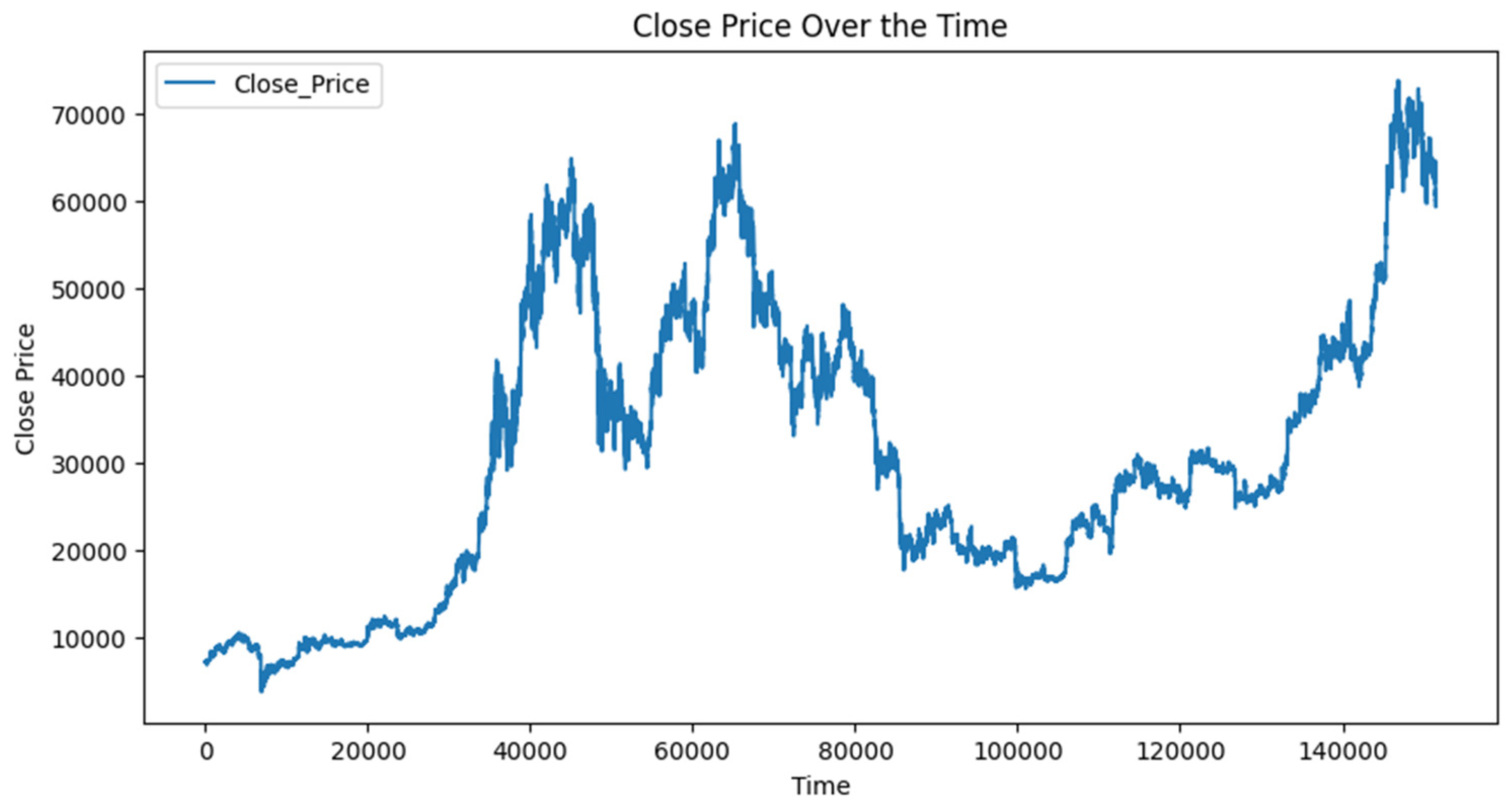
Figure 2.
Autocorrelation Function Plot of 15-minute Time Frame Bitcoin Closing Prices.
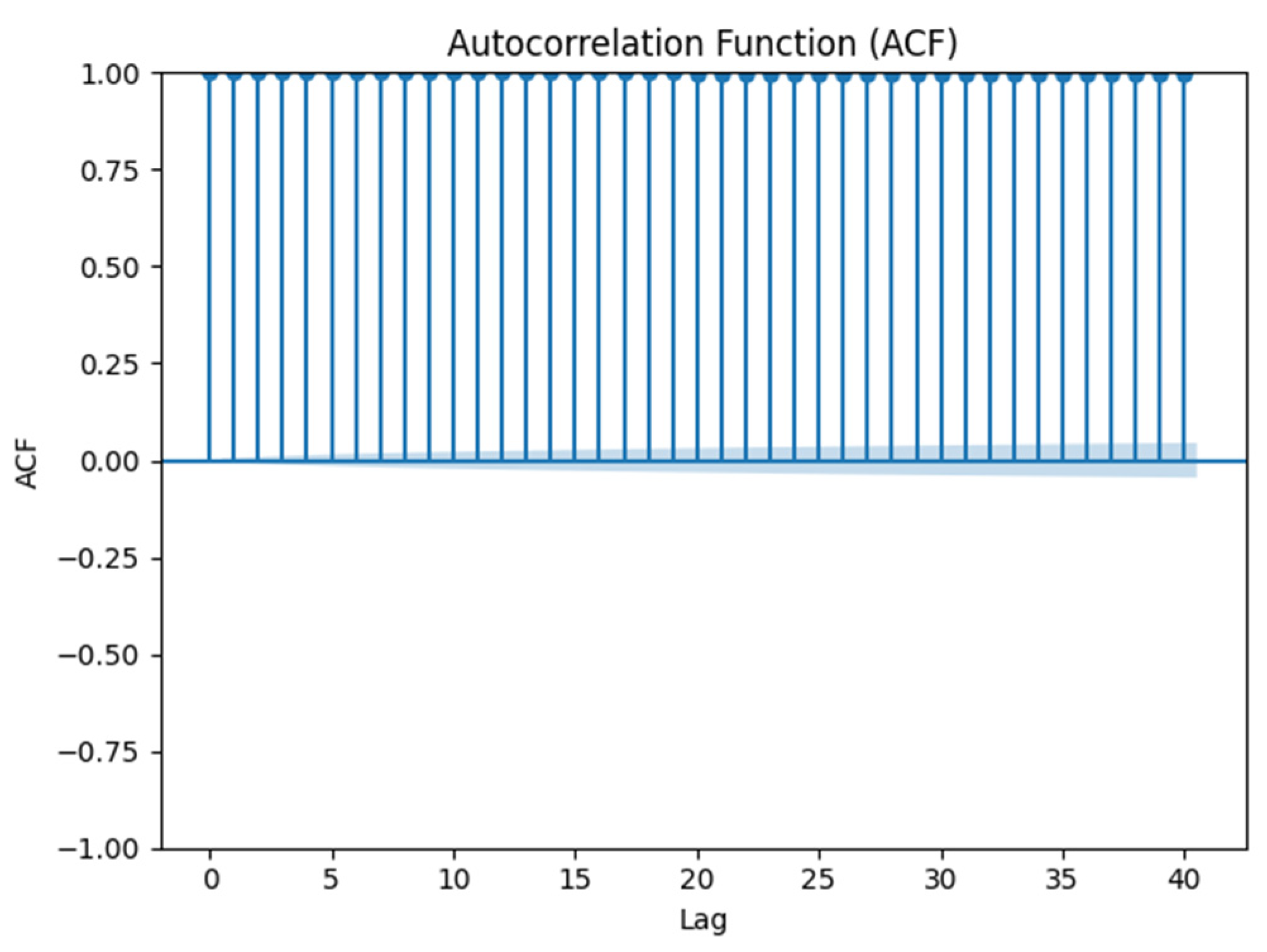
Figure 3.
Historical Data of 15-minute Time Frame Bitcoin Percentage Difference Closing Prices.
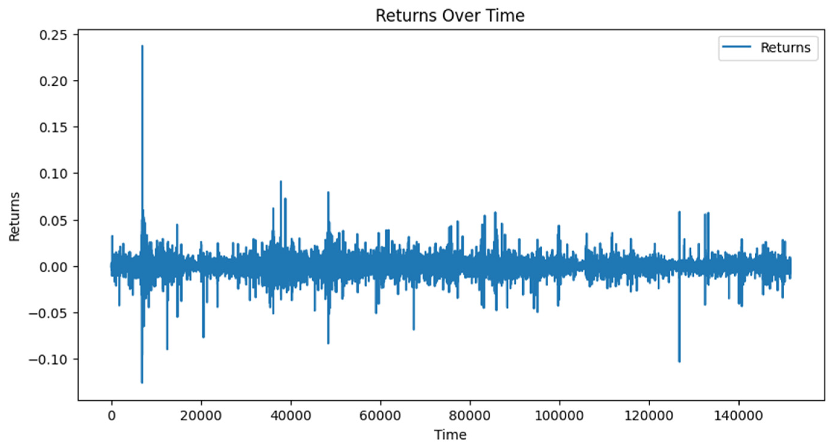
Figure 4.
Partial Autocorrelation Function Plot of 15-minute Time Frame Bitcoin Percentage Difference Closing Prices.
Figure 4.
Partial Autocorrelation Function Plot of 15-minute Time Frame Bitcoin Percentage Difference Closing Prices.
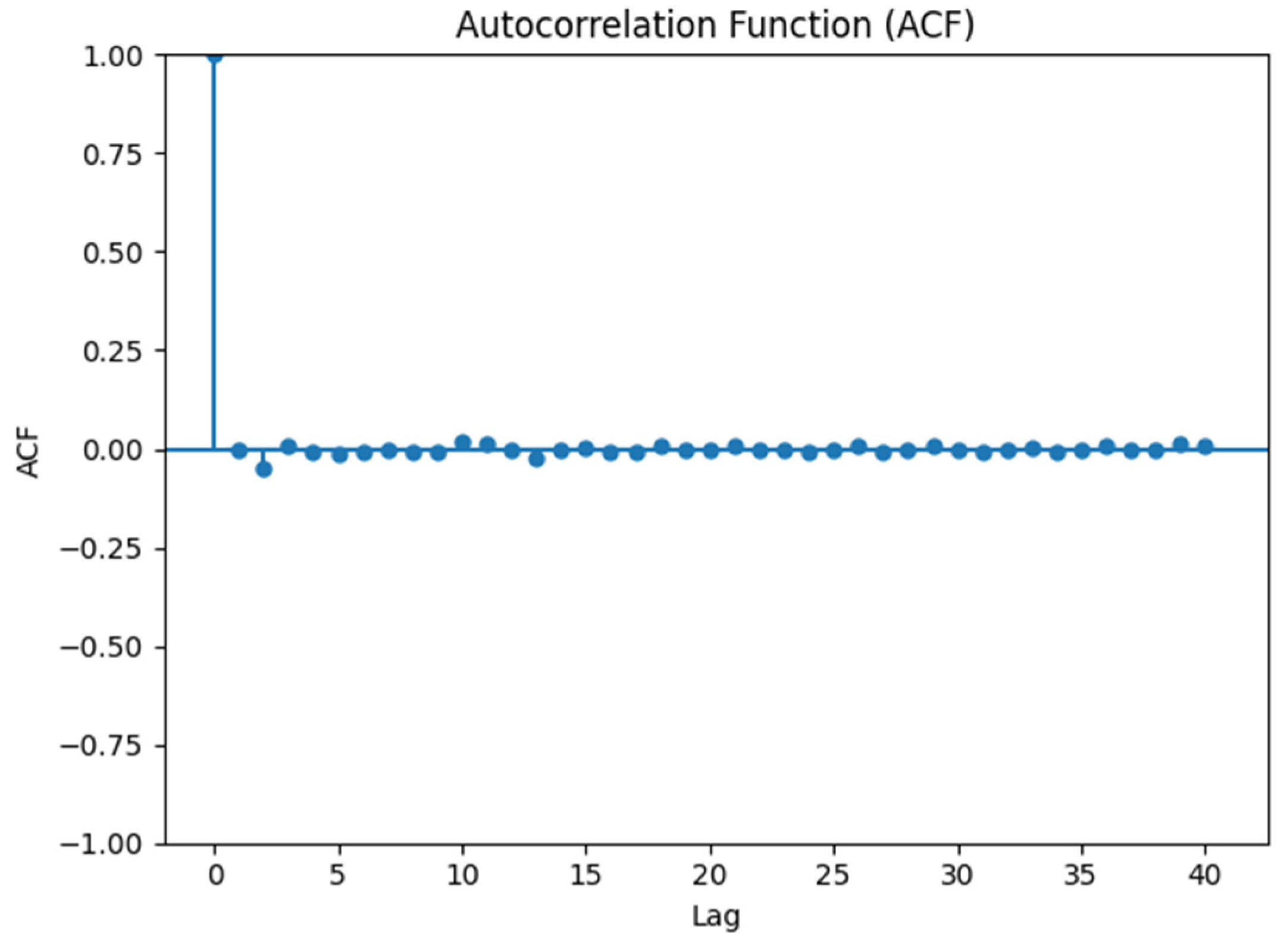
Figure 5.
Flowchart of Logic of the Trading System.
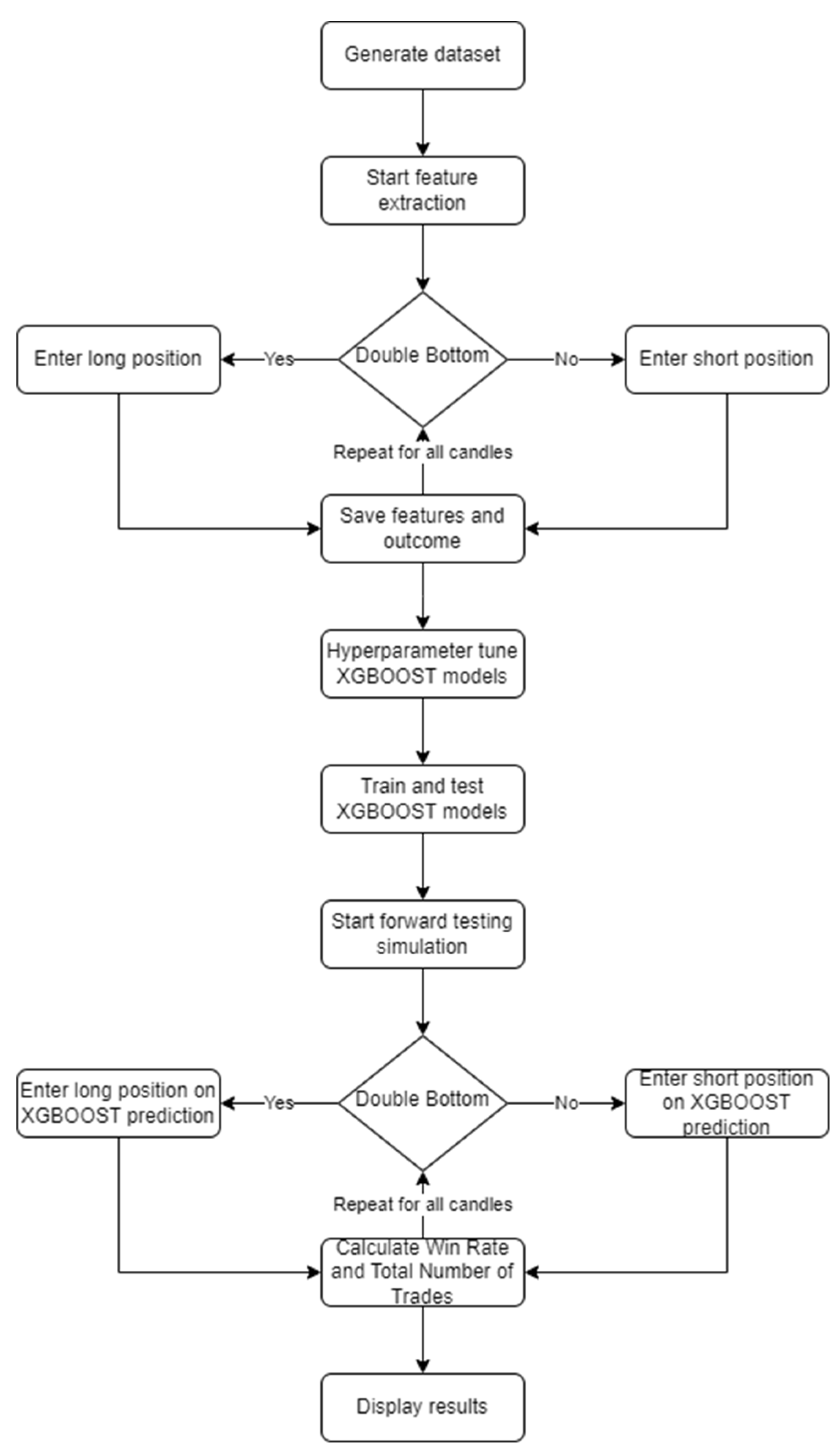
Table 1.
Results of Augmented Dickey-Fuller Test on 15-minute Time Frame Bitcoin Closing Prices.
| Statistic | Value |
| ADF Statistic | -1.2713 |
| p-value | 0.6422 |
| Critical Value 1% | -3.4304 |
| Critical Value 5% | -2.8616 |
| Critical Value 10% | -2.5668 |
Table 2.
Results of Augmented Dickey-Fuller Test on 15-minute Time Frame Bitcoin Percentage Difference Closing Prices.
Table 2.
Results of Augmented Dickey-Fuller Test on 15-minute Time Frame Bitcoin Percentage Difference Closing Prices.
| Statistic | Value |
| ADF Statistic | -44.2766 |
| p-value | 0.0000 |
| Critical Value 1% | -3.4304 |
| Critical Value 5% | -2.8616 |
| Critical Value 10% | -2.5668 |
Table 3.
Results of 15-minute Time Frame, 15-minutes Option Expiration.
| Double Bottom XGBoost | |
| Training Accuracy | 0.631 |
| Validation Accuracy | 0.662 |
| Testing Accuracy | 0.589 |
| Double Top XGBoost | |
| Training Accuracy | 0.713 |
| Validation Accuracy | 0.654 |
| Testing Accuracy | 0.590 |
| Simulation With Machine Learning | |
| Total Trades | 848 |
| Win Rate | 43.63% |
| Simulation Without Machine Learning | |
| Total Trades | 1357 |
| Win Rate | 43.18% |
Table 4.
Results of 15-minute Time Frame, 150-minutes Option Expiration.
| Double Bottom XGBoost | |
| Training Accuracy | 0.773 |
| Validation Accuracy | 0.689 |
| Testing Accuracy | 0.508 |
| Double Top XGBoost | |
| Training Accuracy | 0.669 |
| Validation Accuracy | 0.669 |
| Testing Accuracy | 0.562 |
| Simulation With Machine Learning | |
| Total Trades | 827 |
| Win Rate | 45.22% |
| Simulation Without Machine Learning | |
| Total Trades | 1082 |
| Win Rate | 48.06% |
Table 5.
Results of 15-minute Time Frame, 450-minutes Option Expiration.
| Double Bottom XGBoost | |
| Training Accuracy | 0.563 |
| Validation Accuracy | 0.682 |
| Testing Accuracy | 0.535 |
| Double Top XGBoost | |
| Training Accuracy | 0.685 |
| Validation Accuracy | 0.704 |
| Testing Accuracy | 0.488 |
| Simulation With Machine Learning | |
| Total Trades | 590 |
| Win Rate | 44.58% |
| Simulation Without Machine Learning | |
| Total Trades | 729 |
| Win Rate | 45.13% |
Table 6.
Results of 5-minute Time Frame, 5-minutes Option Expiration.
| Double Bottom XGBoost | |
| Training Accuracy | 0.624 |
| Validation Accuracy | 0.591 |
| Testing Accuracy | 0.500 |
| Double Top XGBoost | |
| Training Accuracy | 0.576 |
| Validation Accuracy | 0.643 |
| Testing Accuracy | 0.570 |
| Simulation With Machine Learning | |
| Total Trades | 1933 |
| Win Rate | 46.61% |
| Simulation Without Machine Learning | |
| Total Trades | 3979 |
| Win Rate | 45.66% |
Table 7.
Results of 5-minute Time Frame, 50-minutes Option Expiration.
| Double Bottom XGBoost | |
| Training Accuracy | 0.558 |
| Validation Accuracy | 0.603 |
| Testing Accuracy | 0.535 |
| Double Top XGBoost | |
| Training Accuracy | 0.972 |
| Validation Accuracy | 0.606 |
| Testing Accuracy | 0.472 |
| Simulation With Machine Learning | |
| Total Trades | 2143 |
| Win Rate | 45.92% |
| Simulation Without Machine Learning | |
| Total Trades | 3160 |
| Win Rate | 47.53% |
Table 8.
Results of 5-minute Time Frame, 150-minutes Option Expiration.
| Double Bottom XGBoost | |
| Training Accuracy | 0.893 |
| Validation Accuracy | 0.632 |
| Testing Accuracy | 0.488 |
| Double Top XGBoost | |
| Training Accuracy | 0.568 |
| Validation Accuracy | 0.609 |
| Testing Accuracy | 0.436 |
| Simulation With Machine Learning | |
| Total Trades | 1744 |
| Win Rate | 50.23% |
| Simulation Without Machine Learning | |
| Total Trades | 2164 |
| Win Rate | 50.18% |
Table 9.
Results of 3-minute Time Frame, 3-minutes Option Expiration.
| Double Bottom XGBoost | |
| Training Accuracy | 0.748 |
| Validation Accuracy | 0.582 |
| Testing Accuracy | 0.505 |
| Double Top XGBoost | |
| Training Accuracy | 0.631 |
| Validation Accuracy | 0.594 |
| Testing Accuracy | 0.529 |
| Simulation With Machine Learning | |
| Total Trades | 3942 |
| Win Rate | 46.50% |
| Simulation Without Machine Learning | |
| Total Trades | 6454 |
| Win Rate | 47.33% |
Table 10.
Results of 3-minute Time Frame, 30-minutes Option Expiration.
| Double Bottom XGBoost | |
| Training Accuracy | 0.586 |
| Validation Accuracy | 0.597 |
| Testing Accuracy | 0.497 |
| Double Top XGBoost | |
| Training Accuracy | 0.522 |
| Validation Accuracy | 0.586 |
| Testing Accuracy | 0.531 |
| Simulation With Machine Learning | |
| Total Trades | 2801 |
| Win Rate | 47.59% |
| Simulation Without Machine Learning | |
| Total Trades | 5145 |
| Win Rate | 48.47% |
Table 11.
Results of 3-minute Time Frame, 90-minutes Option Expiration.
| Double Bottom XGBoost | |
| Training Accuracy | 0.679 |
| Validation Accuracy | 0.614 |
| Testing Accuracy | 0.502 |
| Double Top XGBoost | |
| Training Accuracy | 0.567 |
| Validation Accuracy | 0.594 |
| Testing Accuracy | 0.520 |
| Simulation With Machine Learning | |
| Total Trades | 2647 |
| Win Rate | 47.98% |
| Simulation Without Machine Learning | |
| Total Trades | 3566 |
| Win Rate | 48.65% |
Disclaimer/Publisher’s Note: The statements, opinions and data contained in all publications are solely those of the individual author(s) and contributor(s) and not of MDPI and/or the editor(s). MDPI and/or the editor(s) disclaim responsibility for any injury to people or property resulting from any ideas, methods, instructions or products referred to in the content. |
© 2024 by the authors. Licensee MDPI, Basel, Switzerland. This article is an open access article distributed under the terms and conditions of the Creative Commons Attribution (CC BY) license (http://creativecommons.org/licenses/by/4.0/).
Copyright: This open access article is published under a Creative Commons CC BY 4.0 license, which permit the free download, distribution, and reuse, provided that the author and preprint are cited in any reuse.


