
Submitted:
07 November 2024
Posted:
08 November 2024
You are already at the latest version
Abstract
Google services have shifted the use of technology in our daily lives, enhancing our communication, collaboration and access information. Given this pervasive influence, the aim of this analysis is to compare the predictions of Alphabet’s stock price using various datasets and machine learning models and understand which models perform better, not only in terms of predictive accuracy, but also in terms of explainability and robustness.
To this aim, we have built three different database, considering the existing economic literature and trying to integrate features deriving from the analysis of the context in which the company works and, in particular, R&D costs from Alphabet’s annual financial reports.
We have applied to the database different state of the art machine learning models, ranging from statistical learning models (linear regression), improved with Ridge regularisation, to classic machine learning models such as Gradient Boosting and artificial neural networks, to more recent deep learning models such as recurrent neural networks.
Additionally, the models have been compared in terms of the recently proposed S.A.F.E. AI model, which includes metrics that can assess the Sustainability, Accuracy, Fairness and Explainability of AI application in a unified manner, with a metrics that is related to the Lorenz curve and the Area Under the ROC Curve.
Our empirical findings show that the choice of the best model to employ to predict Google stock prices depends on the desired objective. If it accuracy, the recurrent neural network is the best model. If it is robustness, the Ridge linear model is the most resilient to changes. If it is explainability, the Gradient Boosting model is the best choice.
Keywords:
Google stock prices
; Machine learning models
; SAFE Artificial intelligence
1. Introduction
In this paper, we aim to compare the predictions of Alphabet’s stock price using various datasets and machine learning models and understand which models perform better, not only in terms of predictive accuracy, but also in terms of explainability and robustness.
To this aim, we have built three different database, considering the existing economic literature and trying to integrate features deriving from the analysis of the context in which the company works and, in particular, R&D costs from Alphabet’s annual financial reports.
We have applied to the database different state of the art machine learning models, ranging from statistical learning models (linear regression), improved with Ridge regularisation, to classic machine learning models such as Gradient Boosting and artificial neural networks, to more recent deep learning models such as recurrent neural networks.
The models have been compared in terms of the recently proposed S.A.F.E. AI model (Babaei et al., 2025) which includes metrics that can assess the Sustainability, Accuracy, Fairness and Explainability of AI application in a unified manner, with a metrics that is related to the Lorenz curve and the Area Under the ROC Curve.
The Sustainability metrics measures how resilient are applications of artificial intelligence to perturbations, deriving from cyber attacks or extreme events.To this aim, Babaei et al. (2025) have extended the notion of Lorenz Zonoid to measure the variation in model output induced on different population percentiles, leading to the notion of the Rank Graduation Robustness (RGR) metrics.
The Accuracy metrics extends the well known Area Under the ROC Curve (AUC) to all types of response variables, leading to the Rank Graduation Accuracy metric (RGA), based on the notion of Lorenz Zonoid and on the related concordance curve. Such a measure has allowed the assessment of model accuracy to become more independent on the underlying technology.
The fairness metrics is based on the idea of comparing the Gini inequality coefficient for a model, separately calculated in different population groups. This leads to a Rank Graduation Fairness (RGF) metrics.
Finally, the explainability metrics allows to interpret the impact of each explanatory variable in terms of its contribution to the predictive accuracy, by means of the Rank Graduation Explainability (RGE) metrics.
We have applied the above SAFE AI metrics, excluding fairness, to the predictive output from our alternative models, based on the different databases constructed. Our empirical findings show that the choice of the best model to employ to predict Google stock prices depends on the desired objective. If it accuracy, the recurrent neural network is the best model. If it is robustness, the XGBoost model is the most resilient to changes. If it is explainability, the Ridge linear regression model is the best choice.
The rest of the paper is as follows. The next section Introduces the Models; Section 3 introduces the data we have built for the analysis; Section 4 presents the empirical findings we have obtained applying the models to the data and comparing them in terms of SAFE AI metrics. Finally, Section 5 presents some concluding remarks.
2. Models
The models in this analysis will be based on Deep Learning approaches (Long-Short Term Memory and Feedforward Neural Networks), iterative Machine Learning (Extreme Gradient Boosting) and traditional Statistical Learning methods (Ridge linear Regression). The analysis will use supervised training where both inputs and outputs are given and the predictions will focus on the next day stock price in the output set, which will be compared with the actual output.
2.1. Feedforward Neural Network models
As stated, for example, in Maind and Wankar (2014) neural networks are computational models able to process information similarly to the human brain ,thanks to its large number of tightly interconnected processing elements. See Figure 1.
As shown in Figure 1, a neural network is a network of communicating blocks where, during the training, the model understands how to correctly associate input patterns to output patterns. The choice of this type of model in the analysis is due to the fact that this is the simplest version of neural networks.
According to the recent work of Vasileiadis et al. (2024) the main types of neural network architecture are: Feedforward (FNN), Convolutional (CNN) and Recurrent Neural Networks (RNN), where the latter is a subset of the FNN. In fact, for FNN the information (Figure 1) flows in one direction, from the input layer through the hidden layers to the output layer with no feedback loops or cycles. The main features consist of the layered structure where the hidden layer takes the weighted sum of the outputs from the previous layer and if it is higher than a certain threshold it passes it to the next layer. For further information see Feed Forward Neural Network by DeepAI (last update November 5th 2024). The model proposed in this analysis represents a sequential model consisting of two hidden layers, each with 50 neurons and a single dense layer with one neuron for the output. The training model minimizes the mean squared error and enhances the efficiency of training through its optimizer. We remark that the choice of the number of hidden layers and neurons are arbitrary.
2.2. Long Short-Term Memory Model
In the domain of sequential data processing, the Long-Short Term Memory (LSTM) model is an enhanced recurrent neural network (RNN) whose aim is to capture long-range dependencies while modelling temporal sequences. Vasileiadis et al. (2024) describe an RNN as perfectly suitable for sequential data, like time series scenarios, where data sequence is paramount. The presence of circular links allows the understanding of temporal dependencies and context. Houdt et al. (2020) state that Recurrent Neural Networks take into account connections that loop back on themselves maintaining a hidden layer that carry information across steps. It means that previous inputs are remembered allowing to understand the context. The authors also describe the simplest LSTM version that consists of three key components representing memory blocks: a cell, an output gate and a forget gate. The latter was introduced by Gers et al. (2000) to permit the network to reset its memory. At each step the model processes sequences of data keeping track of relevant information over long periods. Hoss and Alireza (2021) note how it sorts the data according to which new information should be added to the cell, which one should be avoided, and which one should be kept to the following steps, this is also called an iterative approach for forecasting. For further information see Sherstinsky’s work (2020). Particularly, in the model considered here to forecast Alphabet’s Close stock price the lookback parameter has been set to 5 days, representing a week of working days and the output is the price for the following day.
Concerning the model architecture, the analysis consists of a reproducible LSTM model presenting two layers. Firstly, the LSTM layers are composed of 50 neurons defining the capacity of the model to learn dependencies. The output shows only the final state and not the entire sequence. The convergence of the model is set to keep signal stability during training. Secondly, the dense layer with a single output neuron is because the aim is to predict a single value in a regression context. The model is compiled minimizing the mean squared error loss function and uses the optimizer to adapt the learning rate during training for enhancing the efficiency of the convergence.
2.3. Extreme Gradient Boosting Model
As Tarwidi et al. (2023) state, XG Boost represents a decision tree-based technique. Unlike the previous models it is not a neural network but an ensemble of decision trees, optimized for supervised learning tasks. A decision-tree involves dividing the predictor space into different regions or segments where the data is progressively split into smaller subsets assigning to each node a decision based on a particular feature. This process is repeated until the optimal decision path is identified and the most influential variable is on the top. The Extreme Gradient Boosting model is an implemented version of the supervised Gradient Boosting algorithm, introduced by Chen and Guestrin (2016). It is an algorithm that creates and combines a sequence of models to give as a result on overall model using the gradient boosting also known as multiple additive regression trees. The main enhancements introduced by the authors Chen and Guestrin, with respect to the Gradient Boosting version, lays in i) the reduction of the risk of overfitting, ii) the improved ability to make accurate predictions, thanks to the use of the second partial derivative of the loss function, iii) efficiency in parallelization of tree construction and consequently efficiency in terms of training time and iv) the capability to handle missing values. It uses the gradient descent method to optimize the loss function, and it regularizes parameters in order to prevent overfitting. The model performed in this analysis employs Bayesian Optimization to search for optimal hyperparameters which are the learning rate, the maximum depth, the subsample of data and the one of features for each tree. The objective function aims to minimize the root mean squared error using cross validation on the training set.
2.4. Ridge Model
Miller et al. (2022) affirm that Ridge Regression is a linear regression method meant to face the problem of multicollinearity among predictor variables. It introduces a penalty term to the regression function, such that the coefficients are not so high. This regularization term, in fact, shrinks all the coefficients towards zero, reducing their variance and stabilizing the model. Unlike Lasso regression, Ridge Regression keeps all predictors in the model, without setting any of them equal to zero such that no feature is eliminated.
More precisely, Gareth et al. (2021) note that like ordinary least squares, Ridge Regression looks for coefficient estimates that minimize the residual sum of squares (RSS). The key point lays in introducing a shrinkage penalty, which reduces the magnitude of the coefficients, pulling them closer to zero. The balance between minimizing the RSS and applying the shrinkage penalty is controlled by the tuning parameter λ. The simplest case is that when λ = 0 and Ridge Regression behaves like ordinary least squares. Increasing λ, the penalty grows, diminishing the coefficients. This regularization helps prevent overfitting, especially in the presence of multicollinearity. However, the penalty is applied to the coefficients, and the intercept remains unaffected, preserving the overall level of the response variable. Cross-validation is typically used to select the optimal value of λ, ensuring the best predictive performance. For further information see Pereira et al (2016).
The model used for Alphabet’s close price prediction introduces a regularization term to the standard linear regression model where λ is arbitrarily set to 1. This way the penalty is moderate and the size of the coefficients is controlled such that they do not become too large. The goal is to strike a balance between fitting the model closely to the data (as in ordinary least squares) and controlling the complexity of the model to avoid overfitting. The chosen regularization helps reducing the variance in the model, particularly focusing on the data being highly correlated or noisy and stabilizes the coefficient estimates without overly constraining.
3. Data
As mentioned before, beyond R&D data, other factors also significantly impact stock price performance. The key features resulting from our economic analysis of the sectors include i) historical trends, ii) volatility, iii) R&D and iv) technical metrics.
For the prediction of Alphabet’s stock price (GOOG), train and test sets have been constructed, taking respectively 80% of the observations against the remaining 20%. The target variable will be Alphabet’s Close price. The first dataset contains the Close price and its lags (from one to five) over the period from June 2014 to May 2024, sourced from Yahoo Finance. To construct the other two datasets the analysis of the potential features is needed. The features are the following:
At the moment there is no evidence about the impact of correlation among the features in machine learning and deep learning models. However, the analysis will also take into consideration this aspect for the second and third datasets. In Figure 2 we plot all such correlations.
From Figure 2 note that the target variable, Alphabet’s Close Price, has a high correlation (0.98) with IXIC (Nasdaq Composite Index) and TRXFLDUSP (Bloomberg U.S. Dollar Total Return Index), but also the ones with Gold Close Price (0.85), difference between High and Low (0.69) and Crude Oil Close Price (0.56) are worth of being noted (Figure 2).
In fact, the choice of the features will depend on their correlation with each other, that will be minimized, and the correlation with the target variable. In the second dataset the aim is to construct models that do not use information directly from financial reports. In the third one, instead, the goal will be to integrate some data from the financial reporting. Before proceeding, we performed principal component analysis, and show the results in Figure 3.
From Figure 3, it becomes evident that the first feature (namely, retGOOG) explains the most variance in the dataset. To optimize the analysis the variables will be divided into 2 separate datasets, both containing historical values directly linked to the stock price (i.e. retGOOG, HlfiddGOOG, OCdiffGOOG, HLprodOC and StdChangeVolGOOG, IXIC, DXYNYB, VIX) but differing in the remaining features. This choice is due to the goal of explaining the target variable using a wider perspective but a general overview of the models using all the features will also be shown. As far as the analysis includes machine learning models that can benefit from more than the first variable, the aim is to capture complex interactions and uncover potential hidden patterns in the data.
Thus, the second dataset, covering the period from September 30, 2014, to May 31, 2024, will include some variables describing the context in which Alphabet works. Through these variables the covered areas are three: historical data and trends (retGOOG, HlfiddGOOG, OCdiffGOOG, HLprodOC and StdChangeVolGOOG), market influences (IXIC, retGOLD, retCrudeOil, and DXYNYB) and volatility and market sentiment (VIX, retGOOG, HlfiddGOOG, OCdiffGOOG, HLprodOC and StdChangeVolGOOG). The combination of internal stock metrics and external economic indicators should lead to a comprehensive view of the stock price context. As a matter of fact, the PCA for this set of features still attributes about 99% of the variance to the first feature and a minuscule portion of the variance (0,00000498%) to the remaining ones. The composition of the explainability of models will be shown later. The correlation matrix for the second dataset shows how there are still some high correlations but only one high value between OCdiffGOOG and HLprodOC of 0,88. As far as there is no evidence of the negative impact of correlated values in machine learning models it will be useful to interpret also the explainability of correlated variables.
In the third dataset the first six variables are the same as in the second dataset but the other four variables have been added from the annual financial reports related to R&D, P/E and TTM Net EPS. The features considered in the models are the following: retGOOG, HLprodOC, StdChangeVolGOOG, IXIC, DXYNYB, VIX, Gold, CrudeOil, retGOOGvsCostRD, VarAdjClosevsRDrev and AdjClosevsTTMNetEPS (see Table 1 for their explanation). The inclusion of both market and financial indicators aims to incorporate many types of information. R&D-related variables are meant to capture the impact of innovation and research investments on stock performance while the other feature is meant to provide potential insights into the company’s valuation and profitability. Performing a model only including R&D data does not seem to be suitable as the trend grasp many different aspects. Furthermore, the revenues generated from R&D investments cannot be precisely declared as their temporal expansion is hard to be identified. As a consequence, only R&D costs will be integrated in the dataset.
The correlation matrix shows only two high values: between retGOOG and VarAdjClosevsRDrev (0,99) and IXIC and Gold (0,9). This way correlated features are not totally avoided but their presence in the dataset is minimized. As previously affirmed, the main limitations of this approach consist of the low granularity of data and its delayed availability.
Considering the similarity of the second and third dataset resembling results are expected. The main comparison will be discussed between the results of the models using the first dataset, on the one hand, and the remaining ones, on the other.
4. Results
The results will be shown by comparing the performance of each model on the three datasets built in the previous Section, trying to understand which one is the best to predict Alphabet’s Close price and to understand how R&D variables can be integrated. The results of the models using all the variables, except for the lags, are shown in Figure 6.
Figure 6 shows, from the resulting performances for the test set, that the Long-Short Term models is the most accurate model among the considered ones. It represents the case in which the difference between train and test metrics is minimal.
More details on the performance of the LSTM model are shown in Figure 7.
4.1. LSTM
From Figure 7 Looking at the LSTM model, it is possible to note a decline in the results going from the first to the third dataset (Figure 7). The best fitted dataset is the one containing the lags from 1 to 5 of the close price. Its complex structure allows little explainability for predicted value. As it has been shown previously in the datasets, very few features were acceptably explainable in all the scenarios, i.e. IXIC , DXYNYB and the daily return of Gold. R&D variables show explainability values close to zero: retGOOGvsCostRD has 0,0022 and VarAdjClosevsRDrev has 0,0012.
We now focus on the model error. Figure 8 shows the percentage of test observations that actually fall in the predicted confidence intervals, as well as their minimum and maximum values (Figure 8).
From Figure 8, The percentage of values in the predicted interval is 63,90% for Dataset3, the worst case, with 50,83% lower values and only 13,07% higher. For the second dataset the difference between higher and lower percentages is smaller but not as fairly distributed as in the first dataset where they are respectively 50,50% and 49,10%.
These results highlight the fact that the model, although accurate, on average, is not very robust, as predictive accuracy vary when changing the train/test samples. It becomes important to evaluate the model along different metrics, that can measure accuracy, robustness and explainability, possibly in an unified manner. To this aim, we employ the recently proposed SAFE-AI metrics, based on the unifying concept of Lorenz inequality. Figure 9 presents the results for the LSTM model applied to our data.
From Figure 9, it appears that the second dataset shows the highest total explainability (Figure 9) thanks to the Nasdaq Composite index which is the most explainable also in the third dataset but less than in the second one. The difference in the robustness of the fully perturbed set of information is not so relevant among the three cases.
4.2. ANN
We now consider in more detail the ANN model. The ANN model, except for the second dataset, shows a good overall performance (Figure 10), slightly worse with respect to the LSTM model for the first dataset but more accurate for the third one. As it occurs for the Long-Short Term Memory model, the IXIC variable is again the most explainable feature in dataset3.
We consider the predicted confidence intervals, in Figure 11.
From Figure 11, in the first dataset all of the forecasts belong to this interval with 57,46% lower values and 42,54% higher ones. This reflects the fact that outliers are not present. Excluding the second dataset as it could not be used for an effective prediction, the third one of 89,53% of the predictions in the interval highlights how the data is acceptable but more than 58% are greater values so the choice depends again on the strategy that the readers aim to apply to achieve their goals.
We consider the application of the SAFE AI metrics in Figure 12.
From Figure 12, it is possible to note how despite the near 1 result for accuracy, both explainability and robustness for the first dataset are close to zero. For RGE it denotes the fact that the lags of the Close price do not contribute that much in explaining the future values while the RGR results underline the fact that in a possibly evolving environment the results will dramatically change. As a consequence, the choice between the two datasets could be seen as a trade-off between the mere prediction on the one hand and the possibility of interpreting and trusting the data on the other one.
4.3. XG Boost
We now consider the XG Boost model, in Figure 13.
From Figure 13, the XG Boost model shows even better overall results Still the first dataset is the one with the smallest error metrics. The mean absolute percentage error ranges from 2,64% to 6,60%. Again, the third dataset is the one with the minimum R-squared in the considered scenarios. The most explainable features in the second datasets are IXIC and DXYNYB (0,5581 and 0,0273) while in the third one IXIC, Crude Oil price and retGOOG, respectively 0,1921, 0,0279 and 0,0199.
In Figure 14 we consider the predictive accuracy of the confidence intervals.
Considering the 10% interval (Figure 14) of the observed values it is evident how in all of the three cases the distribution is not symmetric, tending for lower values in the first dataset and to higher values in the others. Looking at the lowest overall value of 74,54%, it results perfectly acceptable.
We now consider the application of the SAFE AI metrics, in Figure 15.
The Safe AI metrics in Figure 15 denote generally good accuracy with values near 1, but a huge difference with respect to explainability. In fact, the value related to the first dataset is close to zero while for the second one it shows the highest value of 0,6297 reached in this analysis and for the third it is high with respect to the other obtained values but still closer to zero than to 1 so not so useful. The main issue concerning this model remains the overall robustness when perturbing the data with the smallest value of 0,0038 and the highest one of 0,3263, actually not acceptable.
4.4. Ridge
The last model, the Ridge one, is the most suitable for all of the three datasets, showing the second highest R-squared (0,98) in this analysis, the one of the first dataset, while the remaining sets of information have values above 0,80 (Figure 16).
The most explainable variable is IXIC with a value of 0,3401 for the second dataset and 0,088 for the third one. In fact, the among 10% interval of the actual values (Figure 17) shows how the forecasts of the first dataset all belong to the interval with a distribution tending to lower values. The second and third datasets, with respectively 86,65% and 84,19%, both denote a high proportion of lower values but the difference with the higher values is smaller.
Further investigating the Safe AI metrics (Figure 18), it is possible to note how accuracy (RGA) and robustness (RGR) are respectively, very close to 1 and exactly 1. In terms of explainability, the best scenario is the one of the second dataset with a value of 0,351 while the remaining sets of information are near zero. Again, the less explainable case is the one of the lags from 1 to 5 of the Close price of Alphabet.
5. Conclusion
Our aim was to predict Alphabet’s stock price taking into consideration as many explanatory factors as possible. To achieve this goal, we have added to the available stock price data R&D information from the annual financial reports, as this is an essential aspect to capture and predict the performance of the company.
We have then compared the most important machine learning models on three different data bases, including one which contains the R&D information (Database3). The models have been compared on the different data not only in terms of predictive accuracy, but also in terms of robustness and explainability, in line with the recently proposed SAFE-AI approach.
Our findings underscore the importance of careful model selection in light of the desired outcomes. If the primary goal is predictive accuracy, all of the models show acceptable RGA values ranging from 0,9625 to 0,9955. If the focus is instead on robustness, the Ridge model seems to be the most suitable choice together with LSTM. Instead, if explainability is prioritized over robustness XG Boost will be the best choice. The trade-off between all those aspects should guide the choice of the model depending on the specific application and goals. If the focus is solely on the closeness of the predictions to the actual values the user will consider LSTM using the first dataset. When other aspects are taken into account the choice is more complex.
For further analysis, the analysis could focus on the performance of hybrid models using both LSTM and XG Boost to integrate explainability, robustness and accuracy and apply it on a dataset also including some technical indicators like moving averages and relative strength index.
References
- Babaei, G., Giudici, P. and Raffinetti, E. (2025). A Rank graduation box for SAFE Artificial Intelligence. Expert systems with applications. [CrossRef]
- Maind, B. and Wankar, P. (2014). Research Paper on Basics of Artificial Neural Network, International Journal on Recent and Innovation Trends in Computing and Communication, 2(1), Pages 96-100. [CrossRef]
- DeepAI (last update November 5th, 2024). Feedforward Neural Network.
- Vasileiadis, A., Alexandrou, E. and Paschalidou, L., (2024), Artificial Neural Networks and Its Applications. [CrossRef]
- Van Houdt, G., Mosquera, C. and Nápoles, G. (2020). A Review on the Long Short-Term Memory Model. Artificial Intelligence Review. 53. [CrossRef]
- Belyadi, H. and Haghighat, A. (2021). Machine Learning Guide for Oil and Gas Using Python.
- Chapter 6 - Neural networks and Deep Learning, Gulf Professional Publishing, Pages 297-347. [CrossRef]
- Sherstinsky, A. (2020) Fundamentals of Recurrent Neural Network (RNN) and Long Short-Term Memory (LSTM) network, Physica D: Nonlinear Phenomena, Volume 404, 2020. [CrossRef]
- Tarwidi, D., et al. (2023). An optimized XGBoost-based machine learning method for predicting wave run-up on a sloping beach, MethodsX, Volume 10, 2023. [CrossRef]
- 3.AI (last update November 5th, 2024) Tree-based models.
- Chen, T., and Guestrin, C. (2016). XGBoost: A Scalable Tree Boosting System. 785–794. [CrossRef]
- Simplilearn (last update November 5th, 2024). What is XGBoost? An Introduction to XGBoost Algorithm in Machine Learning.
- Miller, A., Panneerselvam, J. and Liu, L. (2022) A review of regression and classification techniques for analysis of common and rare variants and gene-environmental factors, Neurocomputing, Volume 489, 2022, Pages 466-485. [CrossRef]
- Gareth James, G., Witten, D., Hastie, T. and Tibshirani, R. (2021). An Introduction to Statistical Learning with Applications in R, Second Edition, pages 237-238. See url: https://www.statlearning.com/.
- Pereira, J.M., Basto, M., Ferreira da Silva, A. (2016) The Logistic Lasso and Ridge Regression in Predicting Corporate Failure, Procedia Economics and Finance, Volume 39, 2016, Pages 634-641. [CrossRef]
Figure 1.
A simple neural network. Source: https://ijritcc.org/index.php/ijritcc/article/download/2920/2920/2895.
Figure 1.
A simple neural network. Source: https://ijritcc.org/index.php/ijritcc/article/download/2920/2920/2895.
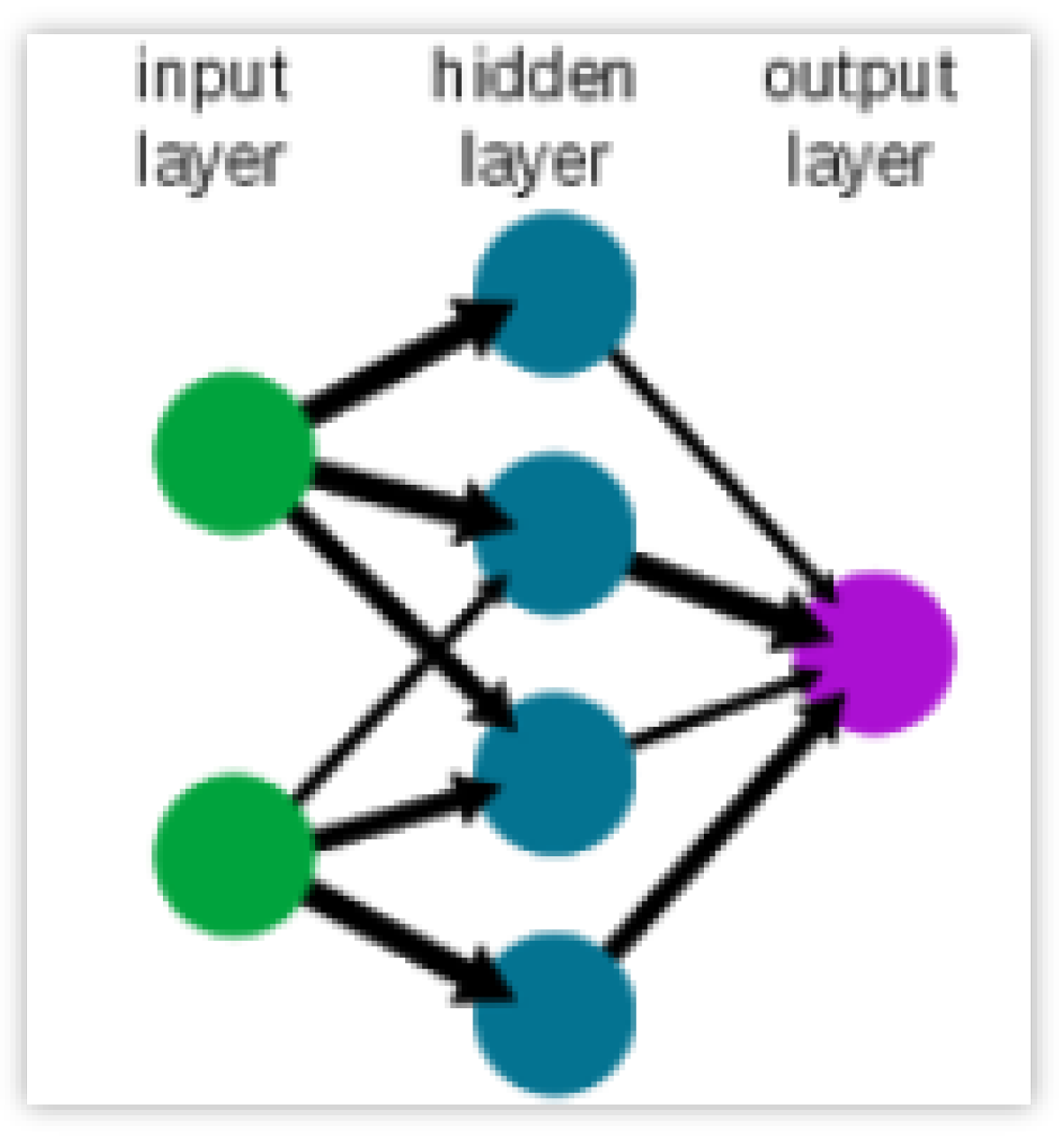
Figure 2.
Correlation among potential features. Source: Yahoo Finance and Bloomberg. Personal elaboration.
Figure 2.
Correlation among potential features. Source: Yahoo Finance and Bloomberg. Personal elaboration.
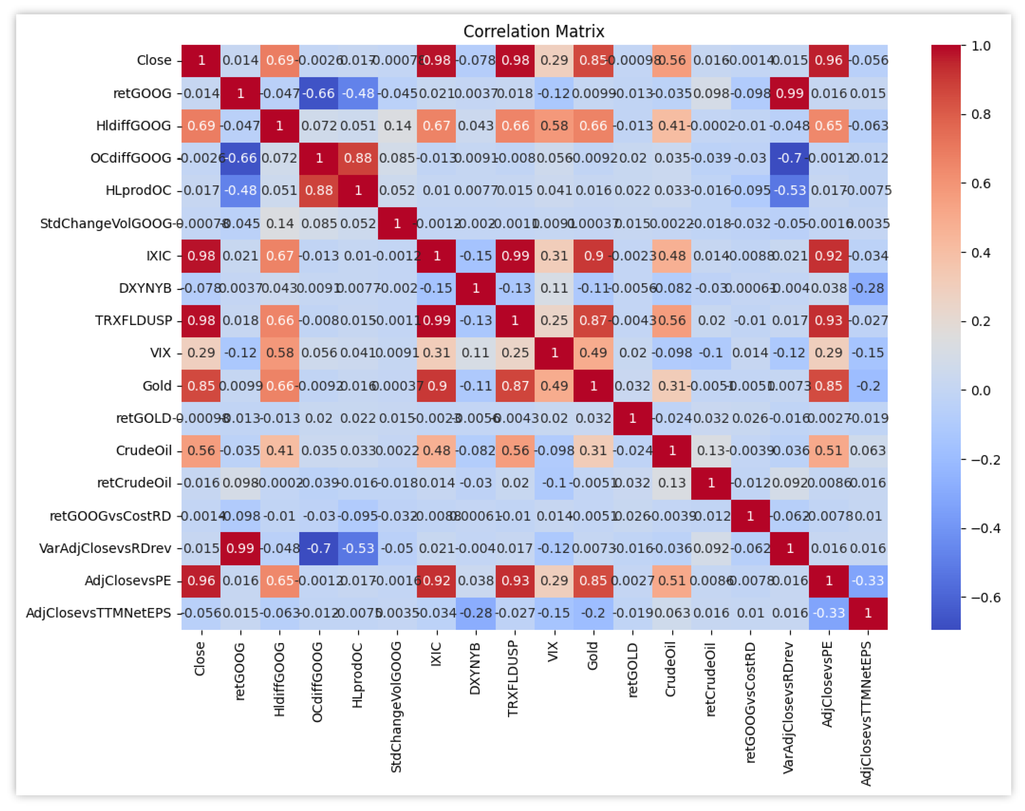
Figure 3.
Principal Component Analysis. Source: Yahoo Finance and Bloomberg. Personal elaboration.
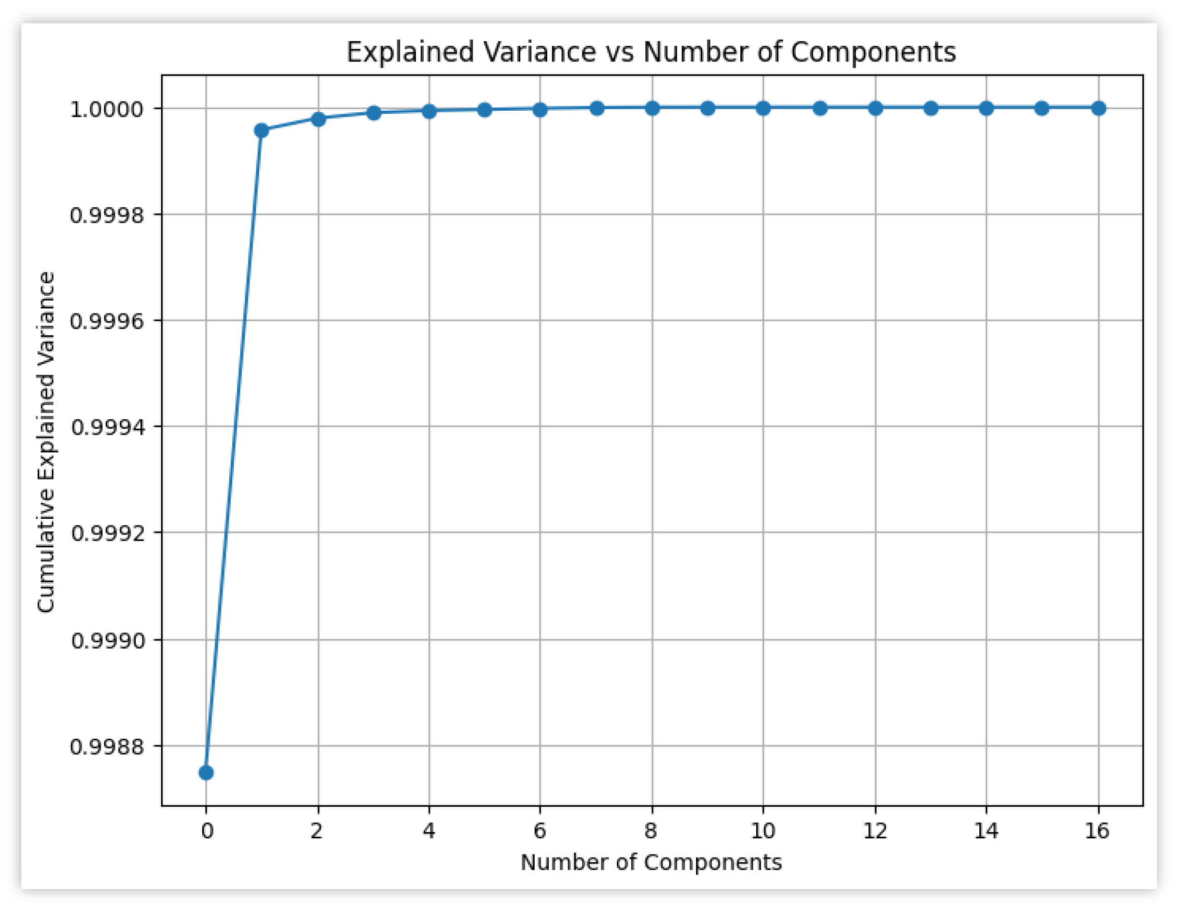
Figure 6.
results of the models using all the features.
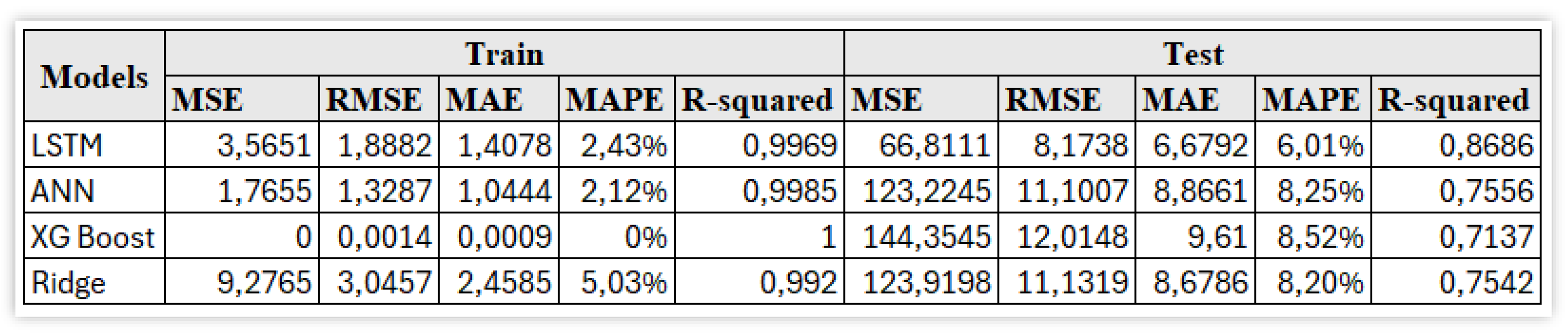
Figure 7.
results for Long-Short Term model.
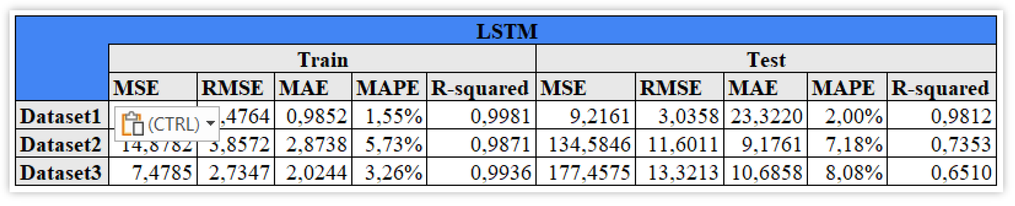
Figure 8.
Custom metric, among 10% interval of the actual values. Personal elaboration.
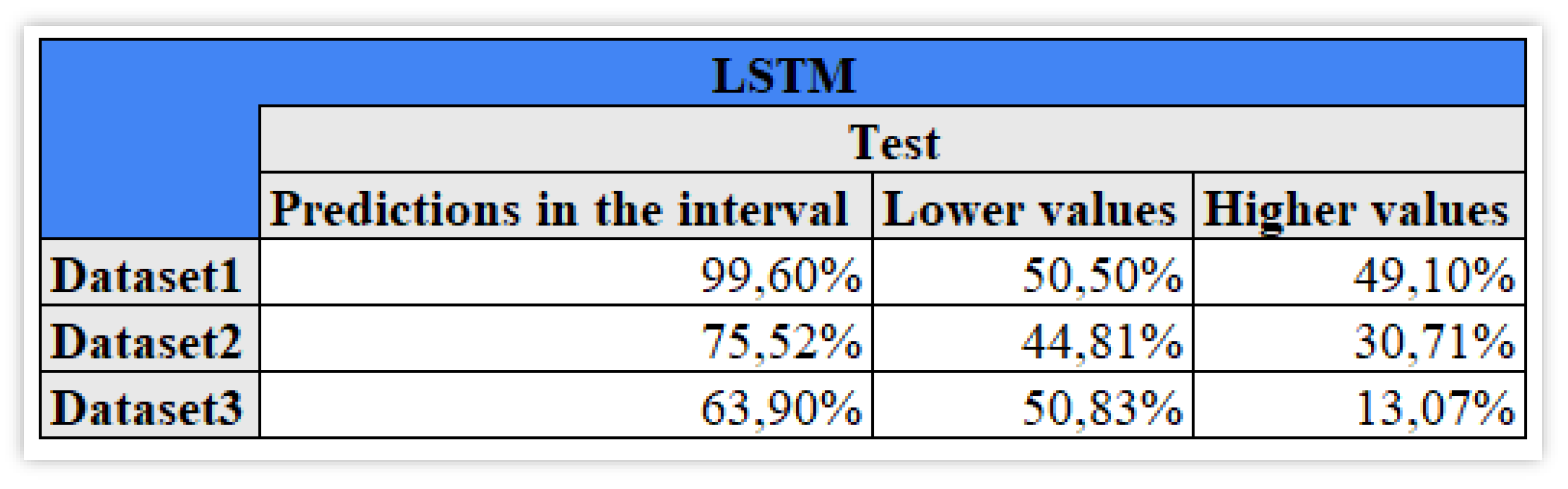
Figure 9.
SAFE AI metrics for LSTM model. Personal elaboration.
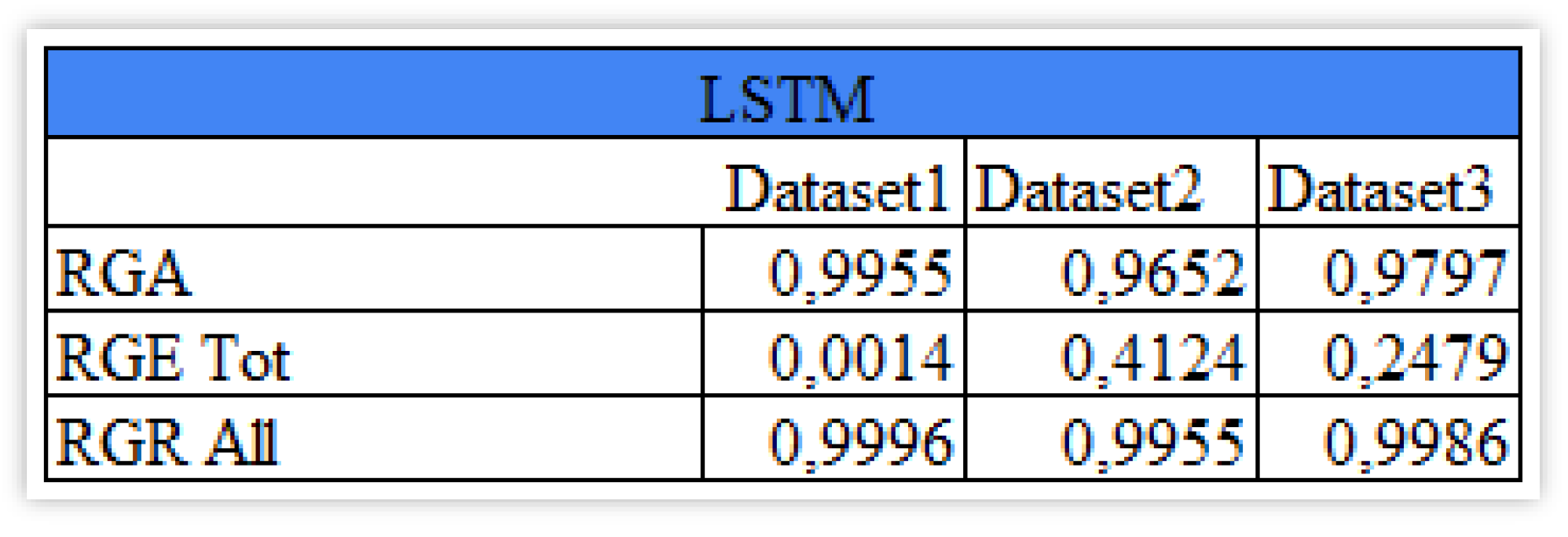
Figure 10.
Comparison of the ANN models. Personal elaboration.

Figure 11.
Custom metric, among 10% interval of the actual values. Personal elaboration.
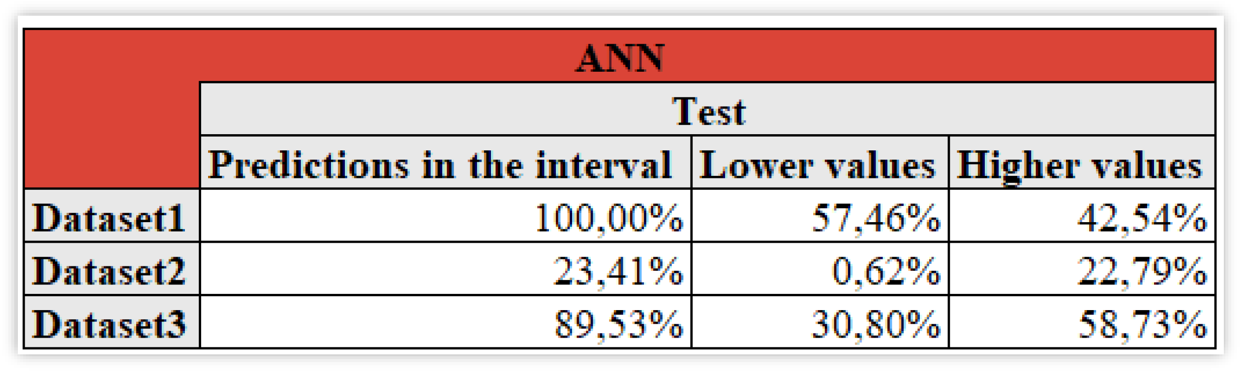
Figure 12.
Safe AI metrics for ANN models. Personal elaboration.
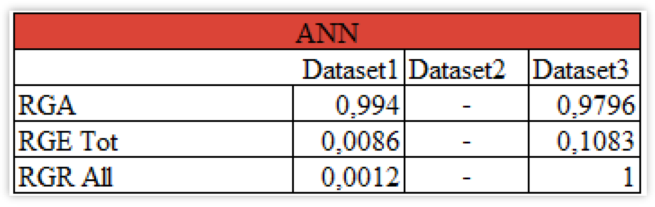
Figure 13.
Comparison of the XG Boost models. Personal elaboration.
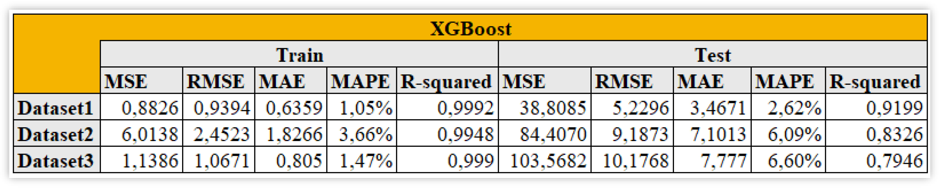
Figure 14.
Custom metric, among 10% interval of the actual values. Personal elaboration.
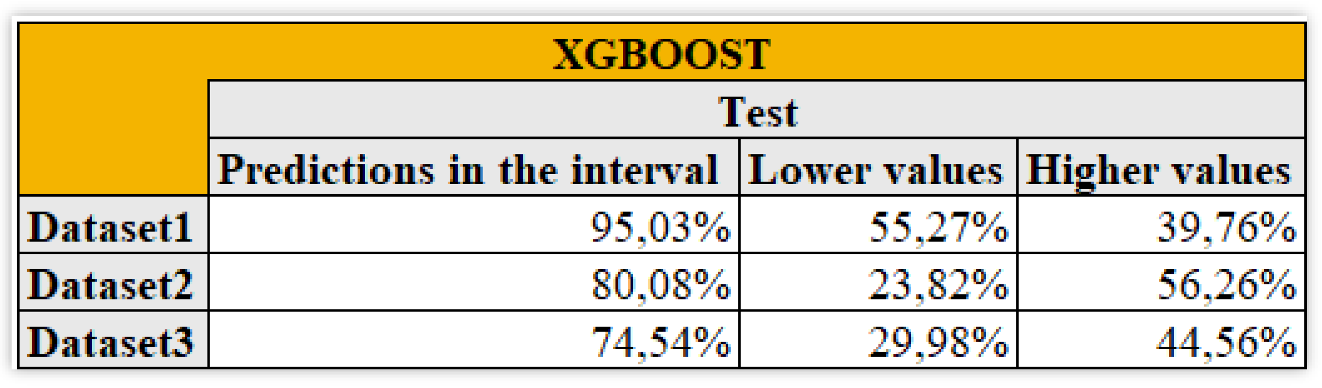
Figure 15.
Safe AI metrics for XG Boost model. Personal elaboration.
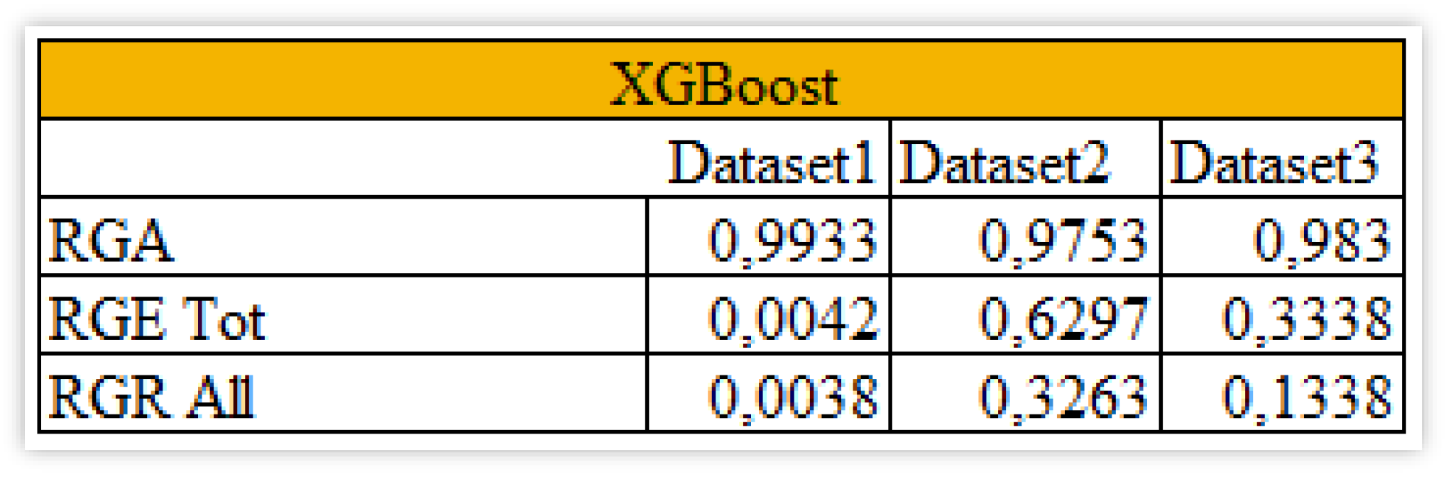
Figure 16.
Comparison of the XG Boost models. Personal elaboration.
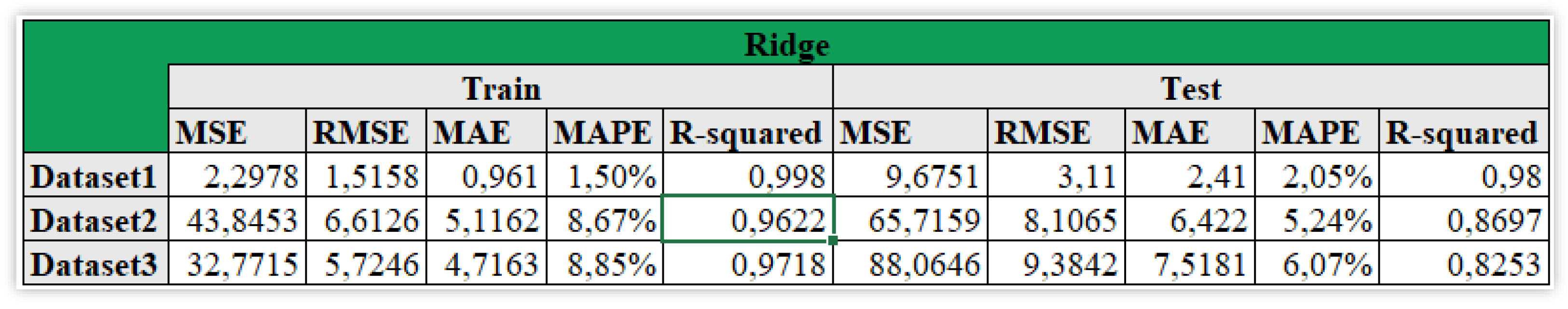
Figure 17.
Custom metric, among 10% interval of the actual values. Personal elaboration.
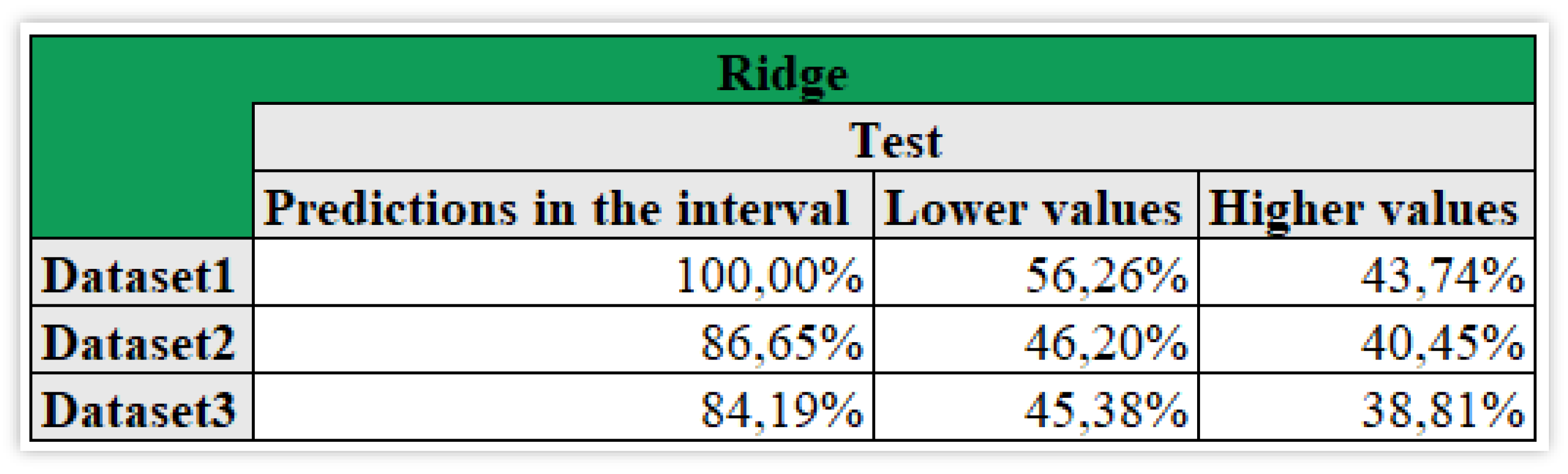
Figure 18.
Safe AI metrics for Ridge model. Personal elaboration.
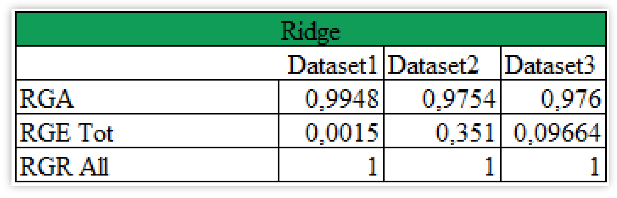

Table 1.
Data to construct the second and third datasets. Source: Yahoo Finance and Bloomberg. Authors’ Elaboration.
Table 1.
Data to construct the second and third datasets. Source: Yahoo Finance and Bloomberg. Authors’ Elaboration.
| Variable | Description |
|---|---|
| retGOOG | Percentage daily return computed as: |
| HldiffGOOG | Difference between high and low daily price: |
| OCdiffGOOG | Difference between Open and Close daily price: |
| HLprodOC | Product between HldiffGOOG and OCdiffGOOG |
| StdChangeVolGOOG | Standardize daily change in volume: |
| IXIC | The Nasdaq Composite Index (^IXIC) including over 3,000 stocks listed on the Nasdaq stock exchange and heavily weighted towards technology companies, sourced from Yahoo Finance |
| DXYNYB | The U.S. Dollar Index measuring the value of the United States dollar relative to a basket of foreign currencies (EUR, JPY, GBP, CAD, SEK, CHF), sourced from Yahoo Finance. |
| TRXFLDUSP | Bloomberg U.S. Dollar Total Return Index. This index tracks the total return of the U.S. dollar in the currency market, factoring in the interest income from holding U.S. dollars relative to a broad basket of currencies. |
| VIX | Volatility Index, a real-time market index representing the market's expectations for volatility over the coming 30 days, sourced from Yahoo Finance. It is derived from the prices of S&P 500 Index options and is calculated by the Chicago Board Options Exchange (CBOE). |
| Gold | Gold Adjusted Close Price on Yahoo Finance |
| retGOLD | Return on Gold adjusted close price: |
| CrudeOil | Crude Oil Adjusted Close Price on Yahoo Finance |
| retCrudeOil | Return on Crude Oil adjusted close price: |
| retGOOGvsCostRD | Ratio between daily percentage of change in price over the quarterly percentage of change in the previous quarter |
| VarAdjClosevsRDrev | Ratio between retGOOG and the percentage of R&D in terms of revenues related to the previous quarter |
| AdjClosevsPE | Ratio between daily price over PE in that quarter. |
| AdjClosevsTTMNetEPS | Ratio between daily price over TTM Net EPS (Trailing Twelve Months Net Earnings Per Share) in that quarter. This ratio could reflect how the current stock price compares to recent earnings over a rolling 12-month period. |
Disclaimer/Publisher’s Note: The statements, opinions and data contained in all publications are solely those of the individual author(s) and contributor(s) and not of MDPI and/or the editor(s). MDPI and/or the editor(s) disclaim responsibility for any injury to people or property resulting from any ideas, methods, instructions or products referred to in the content. |
© 2024 by the authors. Licensee MDPI, Basel, Switzerland. This article is an open access article distributed under the terms and conditions of the Creative Commons Attribution (CC BY) license (http://creativecommons.org/licenses/by/4.0/).
Copyright: This open access article is published under a Creative Commons CC BY 4.0 license, which permit the free download, distribution, and reuse, provided that the author and preprint are cited in any reuse.


