
Submitted:
12 September 2024
Posted:
12 September 2024
You are already at the latest version
Abstract
The study compares three machine learning and deep learning models—Support Vector Regression (SVR), Recurrent Neural Networks (RNN), and Long Short-Term Memory (LSTM)—for predicting market prices using the NGX All-Share Index dataset. The models were evaluated using multiple error metrics, including Mean Absolute Error (MAE), Mean Squared Error (MSE), Root Mean Square Error (RMSE), Mean Percentage Error (MPE), and R-squared. RNN and LSTM were tested with both 30 and 60-day windows, with performance compared to SVR. LSTM delivered better R-squared values, with a 60-day LSTM achieving the best accuracy (R-squared = 0.993) when using a combination of endogenous market data and technical indicators. SVR showed reliable results in certain scenarios but struggled in fold 2 with sudden spike that shows high probability of not capturing the entire underlying NGX pattern in the dataset correctly as witnessed with the high validation loss during the period. Additionally, RNN faced the vanishing gradient problem that limits its long-term performance. Despite challenges, LSTM's ability to handle temporal dependencies, especially with the inclusion of On-Balance Volume, led to significant improvements in prediction accuracy. The use of the Optuna optimization framework further enhanced model training and hyperparameter tuning, contributing to the performance of the LSTM model.
Keywords:
Hybrid Model
; LSTM
; Logistic Regression
; Recurrent Neural Network
; Support Vector Regression
; FinBERT
1. Introduction
The prediction of stock market price has been a long-standing challenge for financial analysts and investors. The intrinsic volatility and complexity of financial markets make it difficult to accurately forecast future trends. Traditional models such as linear regression and time-series models like ARIMA are often limited in their ability to capture non-linear and sequential dependencies within the data [1]. This has led to the growing use of machine learning (ML) and deep learning (DL) techniques for stock market forecasting. The NGX All-Share Index, a key indicator of stock market performance in Nigeria, provides a robust dataset for evaluating the effectiveness of different forecasting models. In this study, we compare three models: Support Vector Regression (SVR), Recurrent Neural Networks (RNN), and Long Short-Term Memory (LSTM), to identify the most effective model for predicting market prices. Each model brings unique advantages: SVR is known for its robustness in small datasets and simple tasks, while RNN and LSTM excel in handling sequential data due to their inherent architecture. SVR operates by mapping input features into two-dimensional spaces using kernel functions, allowing it to capture market relationships. However, it can struggle with time-series data where past information strongly influences future trends. RNN is a type of deep learning model that is designed to capture sequential data, but suffers from the vanishing gradient problem, which limits its ability to retain long-term dependencies. LSTM, an extension of RNN, solves this issue by introducing memory cells that store relevant information over longer periods [2]. This makes it ideal for time-series forecasting. In this research, we used the NGX dataset, which contains historical price data along with technical indicators such as moving averages and On-Balance Volume. These indicators are essential in understanding market behavior and enhancing predictive accuracy. Additionally, models were evaluated using various error metrics such as MAE, MSE, RMSE, MPE, and R-squared. R-squared is particularly important as it measures how well a model explains the variance in the data, making it a crucial metric for comparing models' overall performance. The study employed Optuna, an optimization framework, to fine-tune the hyperparameters of each model. The training process involved time-series cross-validation, which ensures that models are trained and tested on temporally consistent data. Python and its libraries were used for implementing and training the models. This provides flexibility and efficiency in managing the computational requirements.
To provide a clearer understanding of the current research and position the study within the academic field, a detailed Literature Review Table (Table 1) is created. This table presents the various data analysis techniques previously used in stock price prediction research, highlighting their pros and cons. Furthermore, the performance of the three models will be compared with these established methods, showing their ability to capture market trends effectively and improve prediction accuracy.

Table 1.
Literature Review.
| Literature Info | Data | Significance | Contrast | |
|---|---|---|---|---|
| Processing Methods | References | This Work | ||
| Abuein, QQ. et al. [2] | LSTM and Support Vector Regression (SVR) | LSTM showed lower MSE, RMSE, and MAE values compared to SVR. | Limited to two comparative models | SVR struggled with capturing the underlying complex trend, while LSTM outperformed and captured complex trend. |
| Zulfike, MS. et al. [3] | LSTM, SVR, and Vector Autoregression (VAR) | LSTM had higher prediction accuracy and better R-squared score than SVR. | Limited to addition of statistical model with linear assumptions instead of another AI model | SVR had challenges handling large time-series data, while LSTM proved more robust in predicting trends. |
| Lakshminarayanan, JP. et al. [4] | SVM and LSTM | LSTM achieved better MAPE and R-squared scores than SVM. | Limited to SVM that classifies and cannot predict continuous values. | LSTM outperformed due to handling of temporal dependencies, while SVR is not suitable for the NGX dataset. |
| Pashankar, SS. et al. [5] | Linear Regression, Random Forest, SVR | Support Vector Regression demonstrated good short-term predictions. | Limited to machine learning, ensemble learning and basic statistical method | LSTM had better results in long-term prediction accuracy, especially with large datasets. |
Abuein et al. investigated the application of Long Short-Term Memory (LSTM) and Support Vector Regression (SVR) models in time series forecasting. Their study focused on comparing the effectiveness of both models, using error metrics such as MSE, RMSE, and MAE. They found that the LSTM model consistently outperformed SVR with lower error rates, making it more suitable for capturing complex patterns in stock data [2]. The study was limited by its scope, comparing only two models. However, the findings were significant in highlighting LSTM’s strength in handling time series forecasting when dealing with large datasets. Zulfike et al. examined the performance of LSTM, SVR, and Vector Autoregression (VAR) in predicting stock prices. By comparing these models, they found that LSTM achieved better prediction accuracy and a higher R-squared score than SVR [3]. However, the study primarily relied on statistical models like VAR, which are based on linear assumptions. This limited the overall assessment of more advanced AI models that could better capture non-linear relationships. Their work laid the groundwork for exploring more robust models for large-scale time series data, which aligns with the challenges addressed in this work. Lakshminarayanan et al. conducted a comparative study between Support Vector Machine (SVM) and LSTM models for stock price prediction. They demonstrated that LSTM consistently outperformed SVM in terms of Mean Absolute Percentage Error (MAPE) and R-squared scores [4]. However, their study emphasized the limitations of SVM, which is inherently a classification model and not well-suited for continuous prediction tasks like time series forecasting. This comparison further supports the advantages of LSTM in handling long-term dependencies in stock price prediction, a challenge also encountered in our research. Pashankar, SS. et al. [5] focused on evaluating the effectiveness of Linear Regression, Random Forest, and Support Vector Regression (SVR) for predicting stock prices. While their findings indicated that SVR performed well for short-term predictions, their study was restricted to basic machine learning techniques and ensemble methods. This limitation highlighted the need for more advanced models such as LSTM, especially when dealing with larger datasets requiring better long-term forecasting accuracy, a conclusion that mirrors our own work’s findings.
2. Materials and Methods
This study employs historical price data of the NGX All Share Index (NGX) to examine the performance and trajectory of the Nigerian stock market. The NGX is a comprehensive benchmark index that reflects the total market capitalisation of all equities listed on the NGX.
Market Capitalization = Current Share Price X Total Number of Outstanding Share
The NGX Index value is given by the formula:
The dataset spans from January 4, 2010, to June 7, 2024, and consists of 3,573 observations. The NGX dataset pre-processing involved eliminating leading spaces, converting and sorting dates, excising commas, discarding NaN values, converting data to float, and normalising closing price values. The Min-Max scaling technique from Scikit-learn was employed to normalise the NGX dataset. This takes into account its specific attributes as capital market data. The mathematical formula of Min-Max scaler is shown below:
Where: x = Original value,
= Feature minimum value,
= Feature maximum value,
= Scaled value.
The NGX dataset was divided into 85% for training and validation purposes, and the remaining 15% for testing. The model was trained and validated using TimeSeriesSplit. TimeSeriesSplit, a specific scikit-learn timeseries cross-validation (TSCV), was used on a chronologically sorted NGX dataset with of folds (n=5). This approach maintains the temporal relationship between data points, replicates real-world occurrences using unknown future data, and improves the generalisation and prediction accuracy of the model. Each iterative cycle involves assigning a validation dataset and using the previous folds for training. This reproduces the model's ability to generalise strange future facts while being trained. Every time the validated set is iterated, it proceeds to the subsequent set of observations, where n = 5. To prevent data leaking and provide precise evaluation of model performance, all data points are used for training and validation.
2.1. Feature Re-Engineering
The NGX dataset was re-engineered to generate technical indicators using cleaned NGX market data in order to improve predicted accuracy and gain insight into market dynamics. The multi-dimensional approach of including technical indicators to assess price fluctuations, patterns, and trading signals improves the ability of models to detect market swings and provide accurate forecasts [6]. The technical indicators that are added to the historical price and return series for market prediction include the Simple Moving Average (SMA-15 and SMA-45), Relative Strength Index (RSI), Moving Average Convergence Divergence (MACD), Bollinger band (Middle, high and low), and OBV. Bollinger bands represent regions of high or low prices, while RSI confirms whether the market is overbought or oversold. Systematic Moving Averages (SMAs) show the direction of market trend, MACD validates momentum, and OBV use volume flow to forecast fluctuations in stock prices.
Return series is a classic input feature for predicting stock prices. It is the financial gain or loss derived from an investment or stock portfolio within a certain timeframe. Rates of return are determined by calculating the percentage change in market price between two time periods [7]. The calculation is shown below:
The SMA-15 and SMA-45 are statistical moving average measures employed to detect patterns in market data. These figures are derived by computing the average closing prices across time periods of 15 and 45. The combination of the indications can identify crossings, which are useful for making selections into purchasing or selling. The calculation is shown as follow:
For a 15-period SMA:
where “P” is the closing price and “n” is the rolling window period.
SMA15 = P1+P2+⋯+P15
n (15)
n (15)
SMA45 = P1+P2+⋯+P45
n(45)
n(45)
The Relative Strength Index (RSI) is a technical indicator used to measure the speed and extent of price changes. It is often used to identify situations when a market is showing either excessive buying or selling [8]. In this work, the RSI values were computed using window duration of 14 days as shown below.
Relative Strength (RS) = Average Gain
Average Loss
where: Gain= Price increase
RSI = 100-100/(1+RS)
Loss = Price decrease
The MACD is a momentum indicator applied to detect trends and monitor the correlation between two moving averages of stock prices. The computation of MACD entails the utilisation of exponential moving averages (EMAs), which are often shown with a signal line as illustrated below:
Bollinger Bands provide a visual representation of market volatility. This indicates period of instability characterised by substantial price fluctuations and identifying instances of excessive stock purchasing or selling. The gradient between the upper and lower bands varies in response to market volatility. The Bollinger Mid, Upper, and Lower variables utilised in this study indicate the mean, maximum, and minimum levels of volatility in technical analysis. They are computed using the following formula:
where: k = 2 (Bollinger band standard)
Upper Band = Mid Band + (SD × k)
Lower Band = Mid Band − (SD × k)
The use of OBV in this analysis provides a unique approach to using the cumulative total of volume, which modulates the volume in response to price fluctuations by either adding or deleting it. This method is employed to validate pricing trends and provide insights into the magnitude of price swings by analysing variations in volume. OBV is computed by initially calculating the price difference between the current and prior closing prices. The positive discrepancy is included, while the negative discrepancies are subtracted. The cumulative OBV is then calculated by summing or subtracting volume levels based on price changes. By including technical indications into the closing price of NGX, the forecasting accuracy of the suggested AI models is significantly improved. The use of this conversion facilitates the development of more robust and reliable forecasting models capable of capturing intricate stock market changes [9].
The dataset was used in two different approaches to define the input features for the model i.e. classic and OBV inclusion approach. The classic approach involves the usage of return, historical price and price technical indicators as input features while the OBV inclusion approach includes all the features of the classic approach with the addition of OBV indicator
2.2. Algorithm Selection for NGX Market Data
The selection of a specific algorithm type depends on the computational requirements necessary to generate a desired outcome [10]. There are various machine and deep learning that are commonly used for regression analysis but this comparative study used SVR, RNN, and LSTM models due to their unique adaptability, strength, and high performance on different data types in several research contexts. Edward and Suharjito demonstrated that Support Vector Regression (SVR) with the radial basis function kernel excels in properly forecasting Tesla stock prices, therefore establishing its efficacy in financial data modeling [11]. Previous research has demonstrated that LSTM is appropriate for sequential tasks, time series analysis, and natural language processing (NLP). The study conducted by Roy, D shows that LSTM models outperform other models in estimating reference evapotranspiration, thereby offering precise and dependable predictions within agricultural settings [12]. An evaluation of RNN and LSTM showed their effectiveness in capturing intricate temporal relationships in comparison to other machine learning methods [13].
2.2.1. SVR Model Architecture, Development and Training
SVR is a variant of the Support Vector Machine (SVM) technique that is specifically employed for regression task. The architectural components of SVR are kernel function, regularization parameter (C), epsilon (ε) and support vectors. The model separated higher-dimensional data points using the kernel function. This study used the linear kernel for final model training. It is simple, quick, and effective when the input characteristics and target variable are linearly related. The model balances a wide class margin and low error rates with the regularisation parameter (C). The "epsilon" (ε) specifies the area where the model does not penalise errors. It makes the model less sensitive to small data changes and improves performance. Support vectors are the margin-boundary data points that determine the decision boundary (the line or curve separating the data points). The model objective function was created and hyperparameter trial ranges i.e. C: 0.001 – 1000; Epsilon: 0.001 -10; Kernel: linear, poly, rbf, sigmoid; and Degree: 2, 5 if kernel == 'poly' else 3 were suggested for Optuna to explore. This study used Optuna, a hyperparameter optimizer, for its effectiveness, versatility, and user-friendliness, which make it superior to grid and random search. Hyperparameters were evaluated using fold-specific mean squared error. The algorithm finds optimal hyperparameters using Optuna and TimeSeriesSplit. This improves model performance on unknown test data. The training data and target variable were used to fit the SVR model with the optimal hyperparameters during final training. Regression metrics were used on a test dataset not used during training to evaluate model prediction accuracy and dependability.
2.2.2. RNN Model Architecture, Development and Training
The study developed and trained a basic recurrent neural network (RNN) model using TensorFlow and Keras API. The purpose of its creation was to facilitate the acquisition of patterns in time series data by utilizing sequential processing capabilities. The deployment of NGX pricing time series involves this essential need. The research model architecture comprises two recurrent neural network (RNN) layers with alternating dropout layers, as well as a dense layer with a single unit specifically designed for the regression task. The dense layer of the feed-forward neural network (RNN) generates prediction output, while the dropout layer introduces noise during training to reduce overfitting. The input layer shape rotates between a time-step between 30 and 60. NGX domain knowledge was leveraged to establish the data dimensions for each network processing unit. Besides documenting short- to medium-term stock market patterns, we also examined and confirmed concerns about the disappearing and growing gradients of RNNs using 30 and 60 day time increments. The aforementioned problems impede the long-term dependency learning of RNNs. The implementation of a time step, which is the amount of past market observations, is essential for forecasting market prices as stock markets are affected by both current trends and existing patterns [14]. Based on the mid-level performance of the SimpleRNN model, which was evaluated by several manual trials using various combinations of hyperparameters, the Optuna hyperparameter was chosen to optimise the hyperparameters. A set of custom objective functions and constraints were established to assess the performance of the SimpleRNN model using recommended hyperparameter configurations for Optuna. The recommendations included units of 32 and 128; dropout rates of 0.1 to 0.5; batch sizes of 32, 64, and 128; and learning rates ranging from 0.00001 to 0.01. The technique enhanced the overall efficacy and efficiency of the optimisation process. The study employed the Adam (Adaptive Moment Estimation) optimiser to train the model architecture. Adam is capable of integrating the RMSprop approach, which involves modifying the learning rate for each parameter, with momentum control. This concept was supported by Mehmood, F's research on an effective optimisation method for training deep neural networks. Adam was identified as having the benefit of effectively managing sparse gradients and non-stationary targets, which are often encountered in RNN models [15]. This feature renders Adam well-suited for basic RNN models where accurate adjustment of the optimizer is crucial for achieving optimal performance. The study employed mean squared error (MSE) as the error measure for determining the validation loss. Validation of the model on data after the training set was conducted using TimseriesSplit of n=5 folds. Early stopping was employed to monitor the progress of the model, halt training when no improvement was observed, and avoid overfitting while conserving time and resources. The callback interfaced with Optuna to record the validation loss and determine when to initiate pruning depending on performance. Scikit-learn partitioned the dataset and managed cross-validation, NumPy conducted calculations, TensorFlow implemented custom callbacks, and tqdm rendered progress bars. These Python modules facilitated the process of training models, adjusting hyperparameters, and ensuring dependable monitoring and data management. The final model training employed optimised hyperparameters by incrementally increasing the training data at each fold. It was then verified on a 15% fixed-size, forward-moving validation set to demonstrate the enhancement in the model's performance with additional time series data. Finally, the model was tested on the new, unseen test data and evaluation metrics were applied to ascertain the model performance.
LSTM Model Architecture, Development and Training
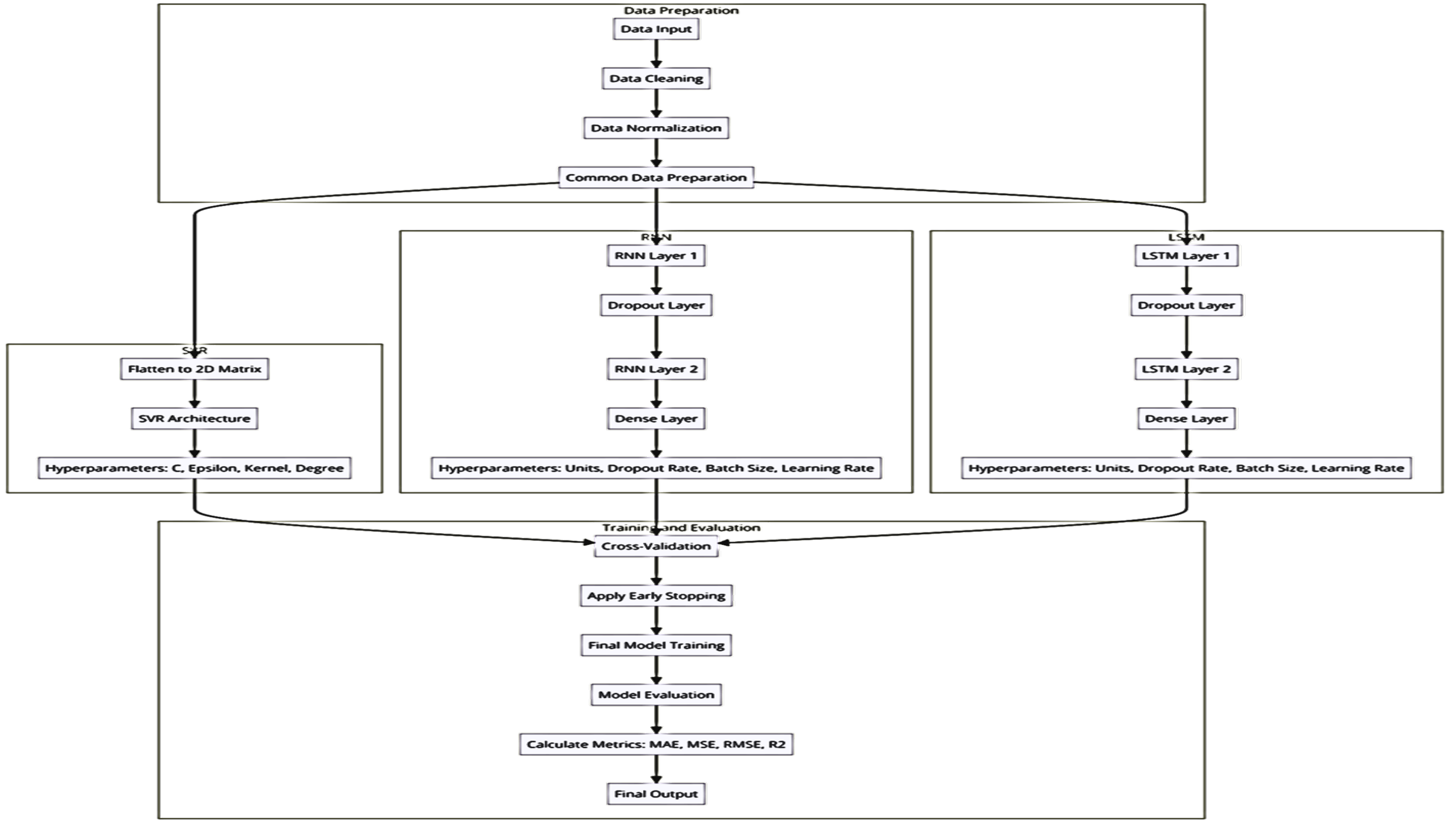
Long Short-Term Memory (LSTM) is a specialized kind of Recurrent Neural Network (RNN) designed to address the challenge of the vanishing gradient problem with sequential input. A gradient vector, often known as a vector of partial derivatives, is a mathematical metric used in model optimisation to quantify the rate at which the output of a function changes in relation to each of its input variables. LSTM utilizes gating methods to preserve data dependencies, control the transfer of information through input, output, and forget gates, and enable the change, storage, and retrieval of the network [16]. The present study created a Long Short-Term Memory (LSTM) model composed of two input layers, a dropout layer, and a dense output layer. The decision to use two input layers instead of the classical one input LSTM layer was made to effectively handle long-term sequence dependencies, address the complexity of market data, and improve the performance of the model. Using a dropout layer as a regularisation technique enhances the generalisation of the model. The adaptability and non-linearity of the dense output layer, achieved via activation functions, effectively capture intricate data patterns and connections. These features are utilised to produce continuous values in regression tasks. The dense layer reduces the dimensionality of information, makes predictions, integrates, and translates learning features to facilitate decision formation. The LSTM model was trained using the same methodologies as the RNN model described above. Figure 1 below shows the three predictive models’ flowchart.
Figure 1.
Flowchart of SVR, RNN and LSTM.
3. Results
The evaluations of predictive models are discussed below. SVR, RNN and LSTM models were trained and tested using historical data from the Nigerian Stock Exchange, with a particular focus on forecasting the NGX All Share Index.
3.1. Support Vector Machines for Regression (SVR)
The NGX dataset's features were converted into a 2-dimensional matrix format for a SVR model. The result below shows the evaluation result of the SVR using regression metrics
Table 2.
Evaluation Result of SVR.
| Best hyperparameters: {'C': 0.2520357450941616, 'epsilon': 0.027026985756138284, 'kernel': 'linear'} |
Best hyperparameters: {'C': 1.1625895249237326, 'epsilon': 0.005801399787450704, 'kernel': 'rbf'} |
|
| Returns & Price Indicators | OBV Inclusion | |
| Cross Validation Training Loss | 0.00110 | 0.00133 |
| Average Final Validation Loss | 0.00197 | 0.0136 |
| Test MAE | 0.0143 (1231.61) | 0.027 (2318.66) |
| MSE | 0.000459 (3396945.36) | 0.00242 (17878018.81) |
| RMSE: | 0.0214 (1843.08) | 0.0491 (4228.24) |
| MAPE (%) | 2.03 | 3.40 |
| R-Squared | 0.99 | 0.95 |
The result from the table above shows the training loss of the classic (0.00110) approach and OBV inclusion (0.00133) method are relatively low. This shows that SVR models performed well on the training data. However, the classic approach training loss is slightly lower and this suggests that SVR fits better during training using classic approach. Also, the classic approach (0.00197) outperforms the “with OBV inclusion’ (0.0136) approach significantly on the validation set. This indicates a lower validation loss generalized better to unseen data during cross-validation. The classic approach has a lower MAE (0.0143) than OBV approach (0.027). This implies it has less average deviation from the actual values, and this is an indication of better predictive accuracy. The MSE of classic approach (0.000459) is lower than the OBV inclusion approach (0.00242). This shows that the model predictions are closer to the actual values and are less prone to errors. RMSE is a measure of the standard deviation of prediction errors. The classic approach has a lower RMSE (0.0214) than OBV inclusion (0.0491). This shows it is more reliable and has smaller prediction errors on average. MAPE is a normalized measure of error. The lower MAPE in the classic approach (2.03%) indicates a better performance in terms of relative error and the predictions are more accurate on a percentage basis. R-squared indicates how well the model explains the variance in the target variable. The classic approach (0.99 =99%) has a higher R-squared value than OBV inclusion approach with 0.95. This explains more variance in the data and is likely a better model. The result of the regression metric above shows classic approach outperforms OBV inclusion approach across all the evaluated metrics. The lower error rates and higher R-Squared value suggest that the inclusion of OBV (On-Balance Volume) did not improve SVR model performance but rather introduced more complexity to the model.
Visual Inspection
The plot of predicted and actual value for classic and OBV inclusion approaches are shown below in figure 2 below:
Figure 2.
Plot of Predictions versus Actual Values on SVR Model.
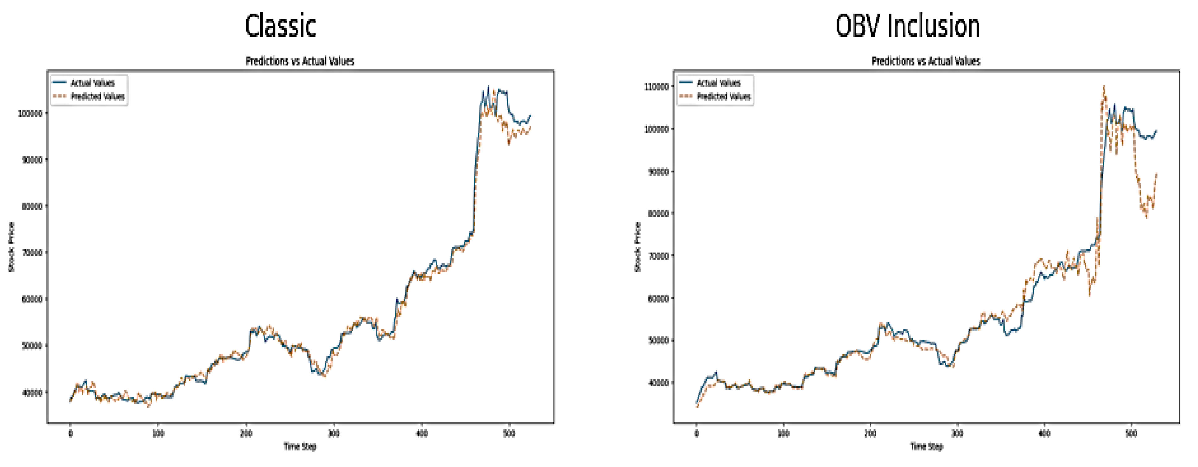
There is a close alignment between the predicted and actual NGX index value of the “classic approach”, most especially at the early and middle segments of the dataset. This shows the effectiveness of the model in capturing general market trends. However, there are some divergences towards the end of the trend, particularly during the peak time. On the other hand, the "OBV Inclusion" approach shows significant divergence between the predicted and actual values, particularly after the stock price peak. This indicates that the inclusion of OBV might be leading to poor model calibration during volatile market periods. SVR model seems to struggle with high volatility and this makes the predicted prices overshoot or lag behind the actual prices, which leads to reduced predictive accuracy.
Diagnostic Evaluation
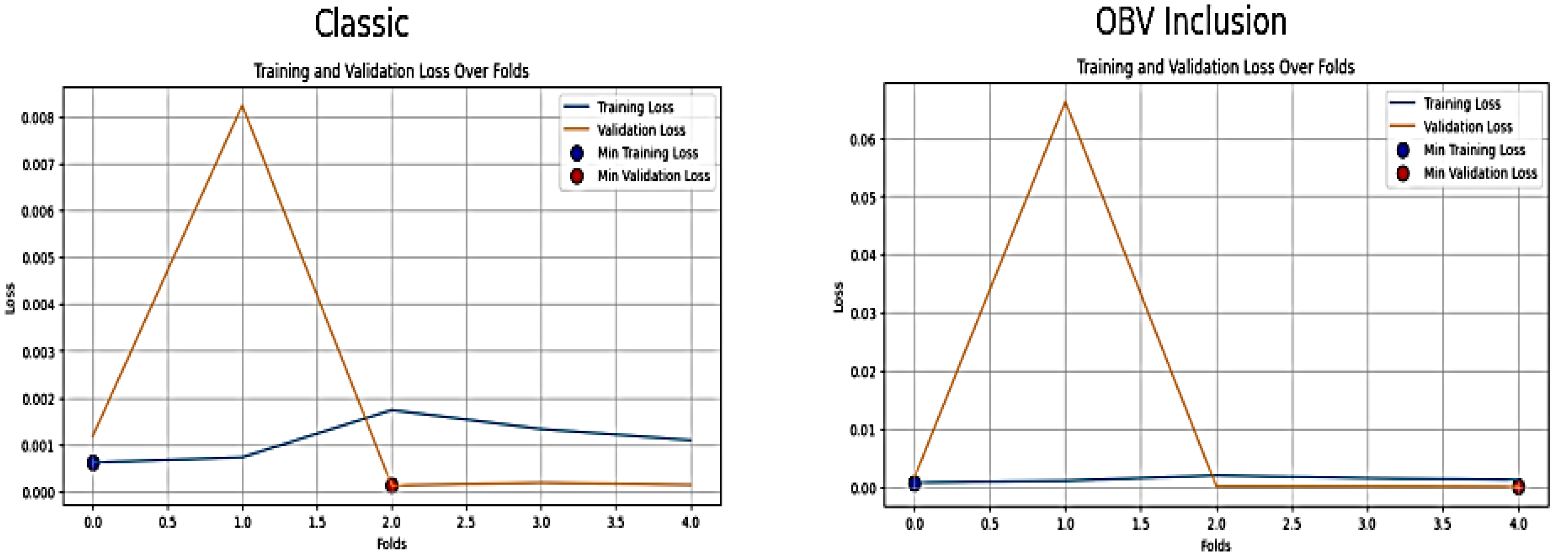
The training loss over folds in Figure 3 below shows that the classic approach has low and relatively stable training loss to reach a minimum loss of 0.000620 at fold 1. The relatively consistent and low loss values suggest that the classic model is performing well in terms of generalization, and with minimal overfitting. The validation loss is also low (average loss: 0.00197) and has a minimum loss of 0.000133 at fold 3. However, there is an observation of a spike in fold 2, which may initially be attributed to an outlier or a subset of data that is fundamentally more difficult to model. Furthermore, the inclusion of OBV in the SVR model seems to introduce higher variability in validation loss (0.0136) compared to the classic approach and has a minimum loss of 0.000093 at fold 5. The presence of a large spike in fold 2 of the OBV inclusion approach could also initially indicate overfitting, poor generalization on that specific subset of the data, the inability of OBV to improve the model stability, the introduction of noise and addition of complexity that SVR could not withstand. These led to further check in order to resolve the spike. The adjustments include data scaling revisit, outlier analysis, hyperparameter tuning re-running with more constraints, a slight increase of regularization, and careful feature re-engineering. All these actions could not create major adjustments because they worsened the situation. This caused the researcher to revert back to the original result plotted below:
Besides, the removal of what is perceived as outliers from NGX time series temporal data is more challenging compared to non-temporal data. This is due to the several inherent characteristics of time series data such as temporal dependency, risk of valuable data loss, and impact on model performance. NGX datasets are sequential in nature, and removal of what is perceived as an outlier might disrupt these temporal dependencies. This will lead to inaccurate analysis of price movement and prediction. Besides, the definition of outlier in time series data is context-based as stock market variation is complex and what is perceived as outlier could represent a significant market event such as a market crash, natural disaster, etc. that should be analyzed rather than removed. The normal value in time series data changes over time due to trends, seasonal patterns, and other factors. According to Tawakuli, traditional outlier detection methods (like Z-scores) may not work well because they assume a static baseline or distribution [18]. Further investigations on the actual cause of the spike of fold 2 in the validation loss led to the findings that there was a high market volatility and non-linearity during the period that could not be captured well by rbf (Radial Basis Function) kernel of SVR. RBF kernel in SVR was specifically designed to capture nonlinear relationships in the data [19]. However, it struggled to capture NGX market patterns at the fold. This could be because stock prices are influenced by a wide range of factors, which include economic events, investor sentiment, and market anomalies, which are often highly volatile, non-stationary, and subject to sudden changes. Despite the regularization put in place and the addition of technical indicators such as moving averages to smoothen and reduce the impact of underlying market trend, SVR model still generated higher validation loss during this fold.
Figure 3.
Training and Validation Loss of SVR Model over Folds.
The actual versus predicted scatter plot of the classic approach below shows a strong linear relationship between the actual and predicted NGX values, with most points lying close to the diagonal line. This shows SVR model is generally accurate in predicting NGX price indices, with relatively few extreme outliers.
Figure 4.
Scatter plot of Actual versus Predicted NGX Index Value on SVR.
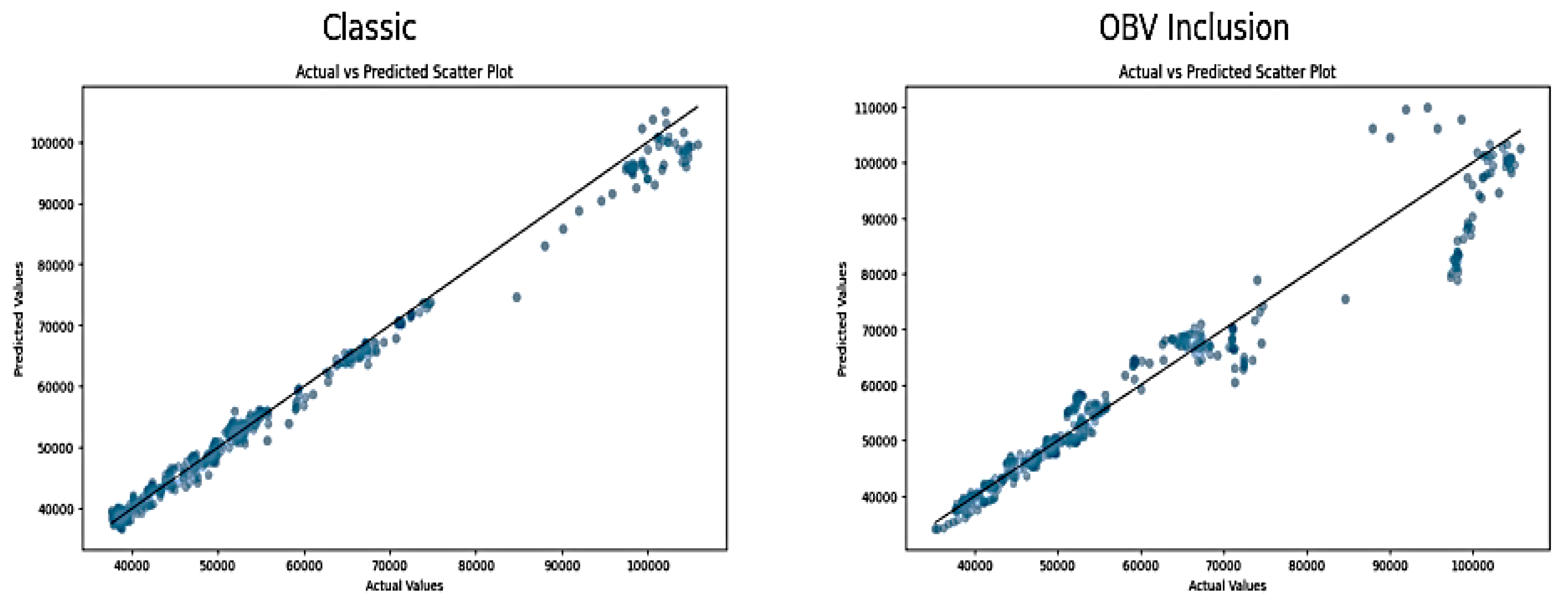
The "OBV Inclusion" scatter plot shows a more dispersed relationship, as shown by several data points that deviate slightly from the diagonal line. The dispersion and occurrence of deviant data points indicate that the On-Balance Volume might be introducing more complexity instead of providing valuable predictive insights. This reduces the accuracy of the model.
Residuals are the differences between the actual observed values and the values predicted by the model. The distribution of residual of classic and OBV inclusion approach are shown in Figure 5 below:
Figure 5.
Distribution of Residual of SVR Classic and OBV Inclusion Approach.
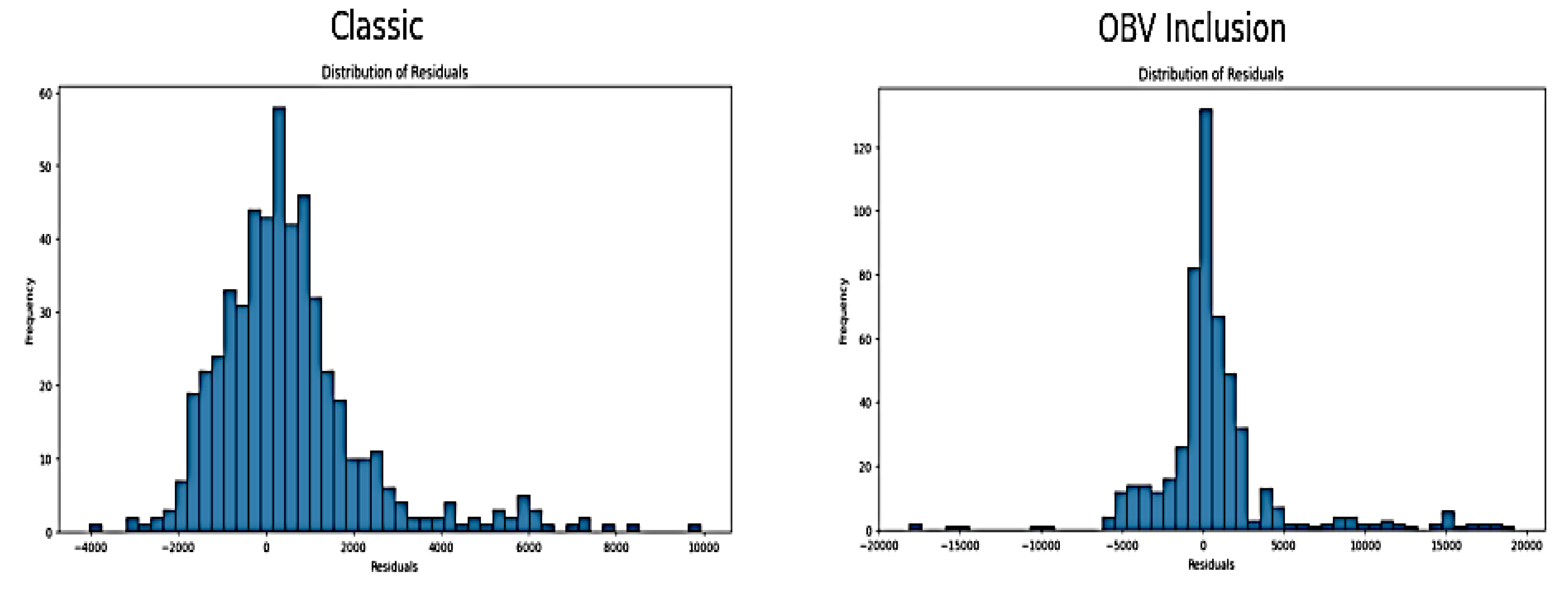
The residual distribution for the "Classic" model is relatively centered around zero, with a bell-shaped distribution. This suggests that errors are relatively normally distributed. It also indicates no significant bias in the SVR model's predictions. On the other hand, the residual distribution for the "OBV Inclusion" approach shows a wider spread and more extreme residuals, especially on the positive side. This skewed distribution suggests that the model is frequently overestimating the NGX value in certain market conditions, which leads to a less accurate model. The classic SVR model approach appears to be the most reliable choice for NGX value prediction. The inclusion of the OBV feature adds complexity that the SVR model cannot handle effectively. Despite the high result generated from the regression metrics, further diagnosis show increased variability in validation loss, poorer alignment in the predictions vs. actual plot, and the wider spread in the residuals distribution from classic approach to the OBV inclusion method suggest that SVR model cannot withstand NGX market complexity, high market volatility & non-linearity, market shock, and market reversal. This makes SVR model not to be the best model for predicting this NGX dataset
3.3.2. Recurrent Neutral Network
The initial best result of SimpleRNN after manual combination of hyperparameters (without hyperparameter optimisation) with input shape of 60 day step-time appears to be unsatisfactory. However, the model managed to perform on a mid-level on a 30 day step-time with SimpleRNN input layer of units of 50, drop-out of 0.2, and dense unit of 1, and with a combination of input features of classic approach. The normalized and transformed original result of the training and validation loses using MSE, and evaluation metrics on the test dataset of the best 30day step-time is shown in the table below:
Table 3.
Evaluation Metrics of the best Un-optimised Simple RNN model.
| Metric Evaluation | 30 day step-time (Normalised value) | Transformed Original value |
| MAE | 0.07483 | 6434.68 |
| MSE | 0.01043 | 77130110.92 |
| RMSE | 0.10213 | 8782.37 |
| MAPE (%) | 11.27 | 11.27 |
| R-Squared | 0.78613 | 0.79 |
The normalised and transformed original value shows high training & validation loss, and high error of the NGX test datasets using evaluation metrics such as MAE (0.0748), MSE (0.010), MRSE (0.10), MAPE (11%) and suboptimal result of 0.79 of R squared. Although, MSE is a differentiable function unlike MAE but the high error of other metrics show inaccuracy of the regression model. MAPE is a percentage error between the model fitted values and the observed data values. According to Lewis, C.D as shown in the table below, the error rate of 11% is a good forecast but is not highly accurate [22].
Table 12.
Acceptable MAPE Values.
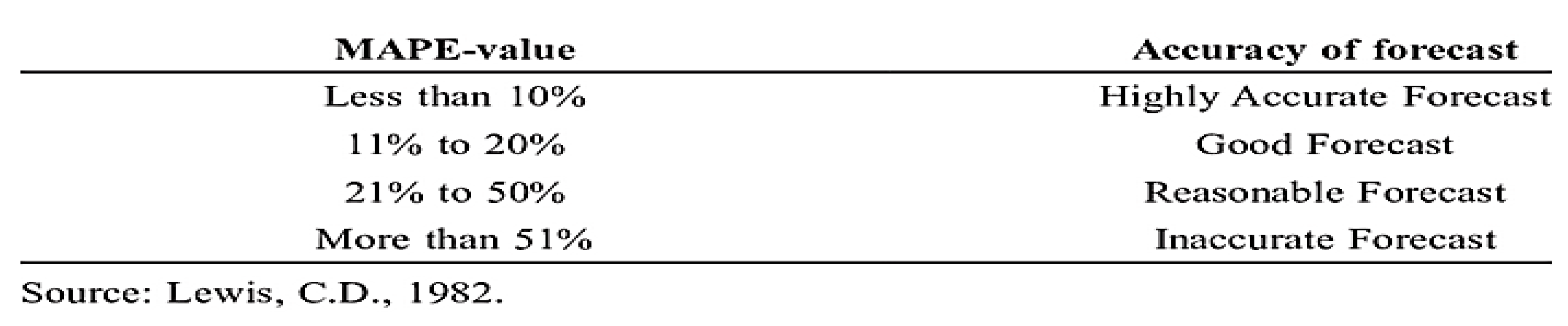
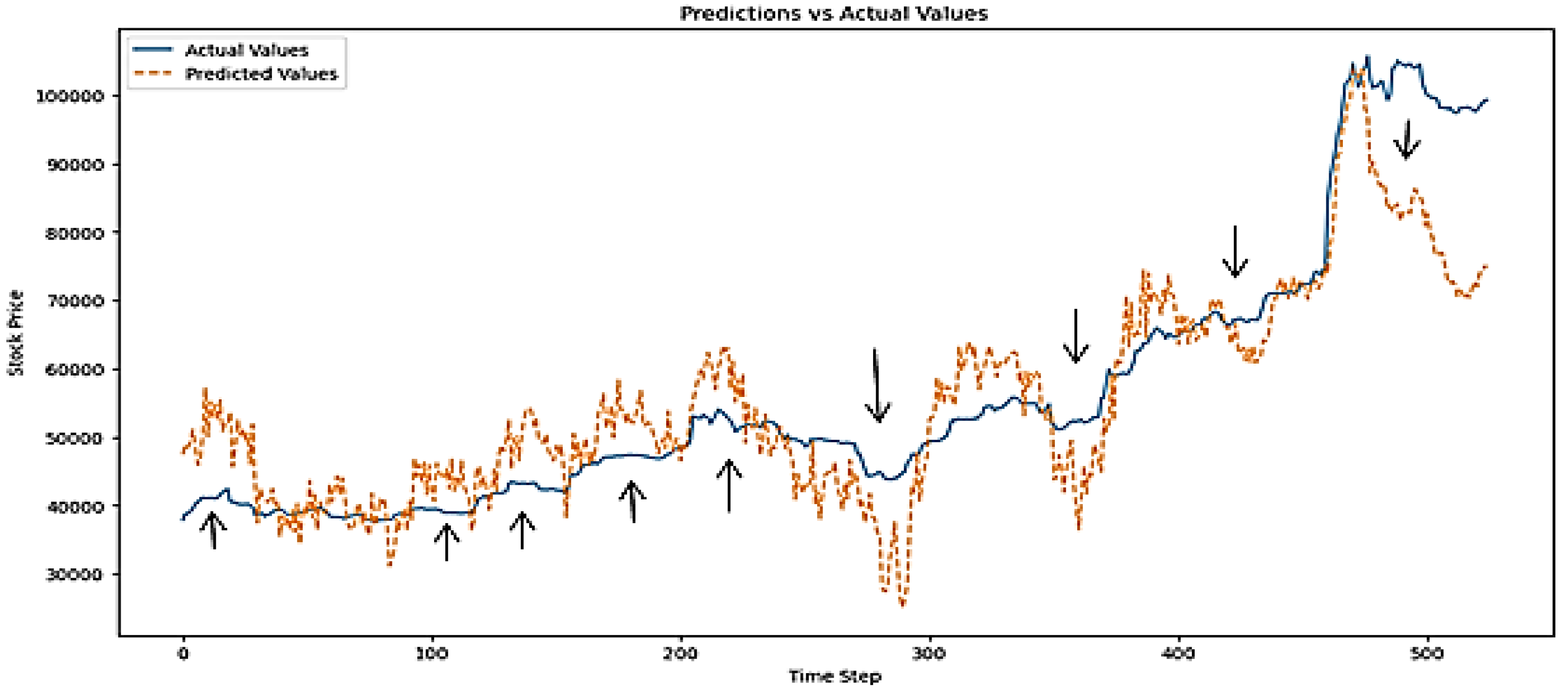
However, the acceptability depends on the industry, application, and specific context. In NGX stock market, a MAPE above 10% is considered inaccurate because of the financial implication and loss on the investment. The error/loss result above clearly shows that SimpleRNN cannot perform accurately on NGX dataset without adoption of hyperparameter fine-tuning technique in real life. Besides, the plot of actual versus predicted of NGX depicted below show the inability of Simple RNN model using classic approach to accurately predict the stock market underlying patterns most especially during volatile periods. The error rate during volatile market period was so high that led to high variation of predicted price from actual price during such periods. The plot of actual versus predicted NGX price value is shown below:
Figure 6.
Plot of Actual versus Predicted NGX Values on Un-optimised RNN Model.
The un-optimised results of SimpleRNN led to the adoption of optimisation technique such as Optuna to fine-tune the hyperparameter and generate the best hyperparameter used in training RNN the model.
A custom objective functions and constraints were defined and suggested for Optuna to search with different sets of hyperparameter combinations (mentioned during model training) to generate the best hyperparameter for the optimisation of evaluation result of SimpleRNN model. The prediction was done using classic and OBV inclusion approach. The financial market has several endogenous variables such as volatility, dividend yield, bid-ask spread, market sentiment but the main endogenous variables are price, volume and returns. Endogenous variables are those variables whose values are determined within a system [23]. Although, majority of the dealing members of NGX uses returns only in ARIMA model for prediction but the study implemented the usage of classic and OBV inclusion method to comprehensively investigate there impact on price prediction with different models. The best hyperparameter generated are tabularised below:
Table 4.
Simple RNN Best Hyperparameter.
| RNN Model | Classic Approach (Input features includes Returns, Historical Price & technical indicators only) | OBV Inclusion Approach (All features and On-Balance Volume) | |||
|---|---|---|---|---|---|
| Best Hyperparameter | 30 day time-step | 60 day time-step | 30 day time-step | 60 day time-step | |
| Units | 122 | 105 | 94 | 79 | |
| Dropout rate | 0.21057927576994717 | 0.15860460902099602 | 0.39808512912645366 | 0.28896636206794524 | |
| Batch size | 32 | 64 | 32 | 64 | |
| Learning rate | 0.00045995847308281305 | 0.004964007144265714 | 0.0033264056797172536 | 0.009618218785212735 | |
The table below shows the result of the evaluation metrics of SimpleRNN model:
Table 5.
Performance of RNN model using Evaluation Metrics.
| RNN Model | Classic Approach (Input features includes Returns, Historical Price & technical indicators only) | OBV Inclusion Approach (All features and On-Balance Volume) | ||
|---|---|---|---|---|
| Losses | 30 day time-step | 60 day time-step | 30 day time-step | 60 day time-step |
| Training Loss | 0.004067 | 0.004150 | 0.005530 | 0.003635 |
| Validation Loss | 0.000125 | 0.000096 | 0.000138 | 0.000119 |
| Test Loss | 0.000388 | 0.000613 | 0.000872 | 0.000982 |
| Test | Evaluation Metrics | |||
| MAE | 0.011321 (973.52) |
0.012490 (1074.05) |
0.019642 (1689.04) |
0.017465 (1501.84) |
| MSE | 0.000388 (2870386.08) |
0.000613 (4533240.36) |
0.000872 (6447080.45) |
0.000982 (7264937.75) |
| RMSE | 0.019702 (1694.22) |
0.024760 (2129.14) |
0.029528 (2539.11) |
0.031345 (2695.35) |
| MAPE (%) | 1.57 | 1.65 | 2.72 | 2.17 |
| R-Squared | 0.992 | 0.987 | 0.982 | 0.980 |
The training loss reflects how well the model fits the training data. As shown in the table above, the classic approach exhibited an increase in training loss from 0.004067 at 30 time steps to 0.004150 at 60 time-steps. This indicates it may be hard for SimpleRNN model to learn with increased time-steps. Salem, F.M study on the RNN limits from system analysis and filtering viewpoints emphasised the vanishing gradient problem attributable to RNN [24]. This study also confirms the vanishing gradient problem of SimpleRNN that will make the model less effective at capturing long term dependencies. However, the addition of OBV to the existing classic approach as input features shows a reduction from 0.005530 to 0.003635. This suggests that the inclusion of OBV to the existing classic method of price prediction may likely assist in ameliorating the effect of vanishing gradient problem of the SimpleRNN on middle to long term. This is a novel discovery as there is no evidence to back it up. It appears the area of research has not been extensively explored in the past.
The minimum loss observed from the time series cross validation is useful for model selection for time series data. The Simple RNN model validation loss reduces from 0.000125 (30 time step) to 0.000096 (60 time step) in the classic method and from 0.000138 (30 time step) to 0.000119 (60 time step) in the OBV inclusion. The lower value seen with both set up show a robust RNN model performance and a good fit (without overfitting) in the different feature set. The comprehensive test loss from regression evaluation metrics show the performance SimpleRNN model on unseen data that do not pass through both validation and testing phase. It also provides an assessment of the model predictive power. There is a close alignment of both tests MSE with validation MSE. This suggests the model generalizes well in real-world situation. However, the test MSE increases from 0.000388 to 0.000613 with classic input features and from 0.000872 to 0.000982 with the inclusion of OBV. The increase in test loss as the time step increases can be attributed to RNN difficulty in generalizing to longer sequences. The transformation of normalised test MSE to original value for ascertaining the significance of the test MSE increase on the original scale show a wide margin from 2,870,386 (30 time step) to 4,533,240 (60 time-step) on classic approach and a marginal increase from 6,447,080 (30 time-step) to 7,264,937(60 time- step) on OBV inclusion. Mean Squared Error (MSE) is known to penalize large errors more heavily. This is due to the squaring of differences which can disproportionately impact the overall error metric. Therefore, it's important to consider other error metrics to gain a more comprehensive evaluation of the SimpleRNN performance. The MAE for the classic approach shows a slight increase from 0.011 (973.5) at 30 time steps to 0.012 (1074) at 60 time steps. In contrast, the MAE for the OBV inclusion approach decreases from 0.02 (1689) at 30 time steps to 0.017 (1501) at 60 time steps. This clearly demonstrates a reduction in the absolute error rate for the OBV inclusion over the long term, in contrast to the classic prediction method, which shows an increase. It also indicates that, despite the reduction, the absolute error for the OBV inclusion remains higher than that of the classic approach when comparing short to medium periods. This could be due to the initial complexity and as the model processes more data over longer sequences, it likely becomes better at leveraging OBV for improved performance. Further research is needed to evaluate the long-term impact of the OBV approach and to confirm the extent of its effectiveness over extended time periods. Even though the MAPE result follows the same pattern as MAE, the variation of error to actual values is between 1.5 % and 2.7%. This is low with OBV inclusion having more error variation. The classic and OBV inclusion method of determining error in model testing show increase in RMSE and this indicates error are larger with more features and longer time steps. The contradiction of RMSE and MAE result of OBV inclusion may possibly be due to specific data segments that are difficult to model accurately by RNN. The R-squared of both approaches remains high with the lowest having 0.98 and highest of 0.99 in RNN model despite variations in metrics.
In conclusion, the addition of OBV to the classic price prediction method reduces training loss on a medium to long term, may likely minimizes the error to actual value on a long term and can capture more market dynamics. However, the error rate within the 30 to 60day time-step (short to medium term) window is slightly higher than the classic approach. This could be the adjustment period required by RNN model to effectively utilize OBV. The result also shows the consistent increase in classic method error rate as time-step increases. This clearly indicates the ineffectiveness of SimpleRNN to capture medium to long term dependencies in financial time series.
Visual Inspection
The plots of actual and predicted NGX value below modelled over a 30 and 60 time step periods. The classic 30 and 60 days’ time-steps predicted values closely follow the actual NGX market values. This shows the RNN has the capacity to capture trends and fluctuations in stock prices and also suggests good model accuracy. Although, the performance of classic 30day time step model have a smoother prediction which confirms short term steps allows RNN to better capture underlying patterns.
Figure 7.
Plot of Actual versus Predicted NGX Price Index on RNN Model.
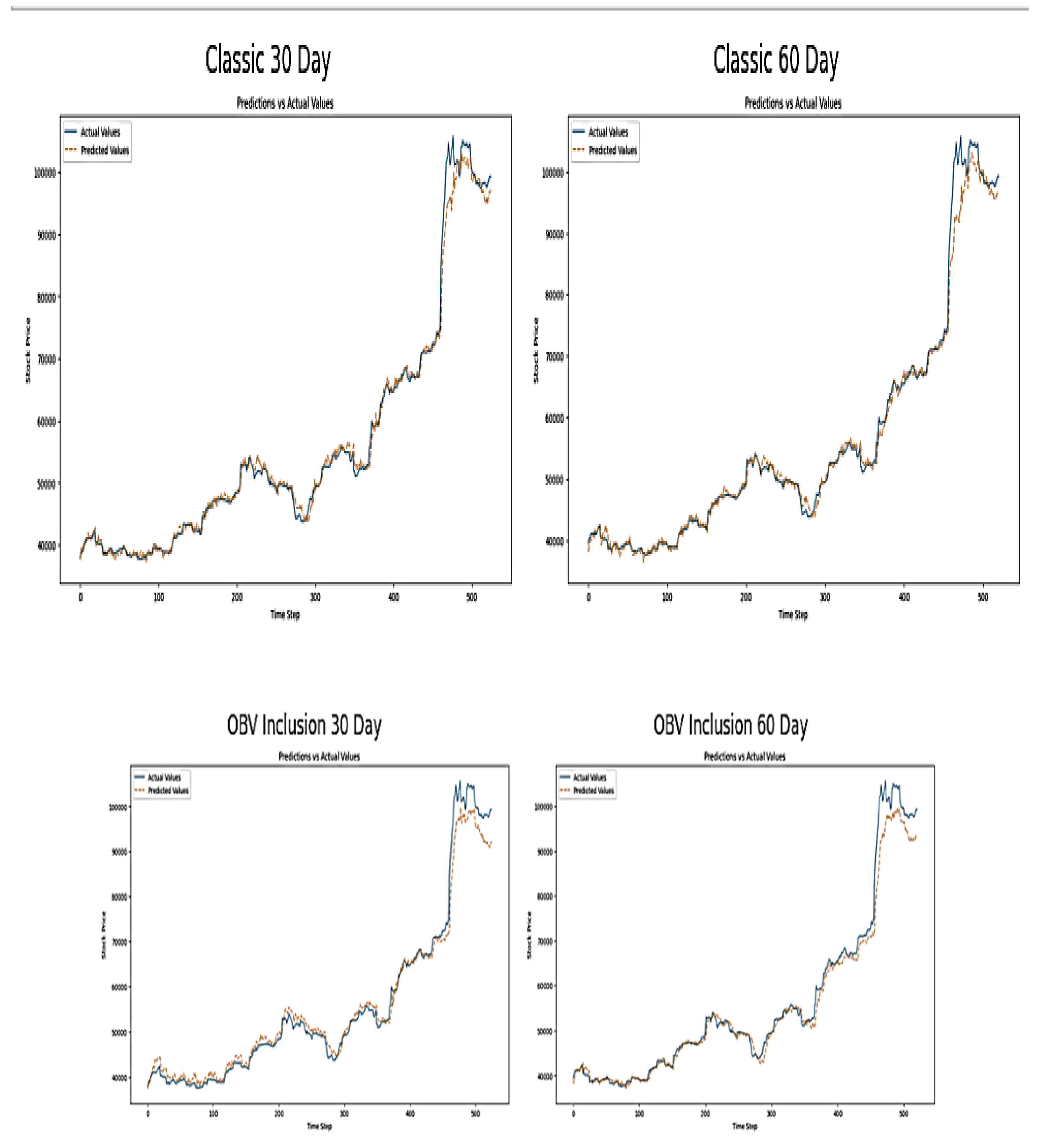
The observation of the plot of actual and predictive NGX index values on a 30 to 60 time step above shows the addition of OBV to the SimpleRNN subjects the model to potential high volatility in their predictions. This will be further confirmed by the scatter plot below. This price movement shows sensitivity to volume changes (which OBV measures) and indicates that OBV assists the model to dynamically respond to significant price movements. The comparison of classic approach with OBV inclusion method appears to make the RNN predictions to be more responsive to sudden changes in the market. This can increase accuracy during the volatile periods and may also introduce noise into the prediction during stable periods. This can be observed by the slightly higher deviations from the actual values towards the end of the OBV graphs.
Diagnostic Evaluation
The plot below shows the training and validation loss for Simple RNN over a series of epoch using classic and OBV inclusion approach.
Figure 8.
Training and Validation Loss over Epoch OF RNN Model.
The training loss of Classic 30 time step in the figure above shows rapid and steep decline in the first few epoch before reaching minimum loss of 0.002479. This suggests the SimpleRNN model is learning quickly from the training datasets. The validation loss displays the same trait as training loss but flattens out before reaching minimum loss. It indicates the model generalizes well on unseen data without overfitting. Also, the training loss of classic 60 time step follows similar pattern to the 30 time step model with a slightly higher initial loss between epoch 0 and 5 before reaching minimum loss of 0.002. This indicates the RNN has challenges in learning longer sequences and with more complexity. The validation loss decreases in alignment with training loss and stabilizes at minimum of 0.00008. This shows good model performance and generalization
The training loss of 30 time step of OBV inclusion started high compared to Classic 30 time step. This indicates initial complexity which was due to the addition of OBV features. However, it decreases quickly to a minimum loss of 0.0055. This implies quick learning of the simple RNN model. However, validation loss starts higher but steadily decreases to a minimum loss of 0.000138. This implies the addition of OBV assists the model in capturing more complex patterns. The training loss of 60 time step of OBV inclusion is similar to classic approach of 60 time step. It starts with a higher loss and reduces hastily to a minimum loss of 0.0036. The shows the inclusion OBV method does not significantly change the learning pattern but make the architecture of the RNN model to be robust. The validation loss reduces in sync with the training loss to a minimum loss of 0.0001. This implies that the RNN model is generalizing well despite the added complexity of OBV. In a nutshell, OBV inclusion to the classic approach provides meaningful information for prediction. Besides, most of the learning starts in the early epochs but the loss reduce as the training progress. This is typical of neural network training where early iterations make significant updates to weights.
The scatter plots displayed below shows the relationship between actual and predicted stock prices by RNN models. These plots are useful for assessing the accuracy and predictive power of models used in forecasting financial market data. The observation of data points cluster near the diagonal line, which represents the line of perfect prediction in 30 and 60 time-step of Classic approach, indicates a strong linear relationship between the actual and predicted values. This suggests a good accuracy of RNN model. The near alignment shows classic approach is good at capturing the underlying trend. However, the 60-day model might offer a slightly baggier cluster around the line, which implies less accuracy with a longer data sequence.
Figure 9.
Plots of Actual and Predicted NGX Price Index Scatter Plot of RNN Model.
The plots of 30 and 60 time steps of OBV inclusion indicate a good connection between actual and anticipated values at the beginning, loosely fitted towards the end and tightly fitted at the end. This shows OBV integration appears to preserve model prediction quality and provide volume related information that complements price data, especially in the 60-day model where data points are closer to the perfect prediction line. The comparison of the four plots shows consistent demonstration of high accuracy with slight differences in the spread of points around the diagonal. Generally, the result suggests robust model performance across varying configurations, and this validates the use of RNNs in financial forecasting. This analysis reflects the RNN's ability to adapt its learning from historical data to predict future values, demonstrating the potential benefits of sophisticated models in financial forecasting.
The residual plots below show the distribution of residuals (i.e. the differences between actual and predicted values) of SimpleRNN models used for predicting NGX prices indices. The Classic approach for 30 and 60 time-step distributions appear positively skewed with a long tail toward right. This shows the gradual decrease in residual frequency as they move from negative to positive values. It reflects occasional large positive residuals with prediction lower than the actual values. The residuals are centered around zero with 60 day plot appearing to have a slightly tighter distribution compared to 30days time step. This indicates that the model’s predictions are generally accurate. The range of residuals that shows variations in prediction for classic 30days is from -4,000 to 10,000 while that of Classic 60 days is approximately -2500 to over 12,500.
Figure 10.
Plots of Distribution of Residuals of RNN Model.
The residual plots of OBV inclusion are similar to classic plots. The majority of the residuals are centred around zero but with different narrow spread. This indicates that on average the model predictions are close to the actual values. The distribution is positively skewed and this implies that there are more large positive residuals than negative residuals. This indicates the model occasionally underestimates the actual values as previously shown in the plot of actual versus prediction. The range of residuals from approximately -2500 to over 10000 indicates variability in the accuracy of predictions across the datasets. The residuals show that the models generally predicts close to actual values as seen with the cluster around zero. It also shows the instances where the predictions differ from the actuals, as shown by the tails. The positive skewedness of the study distribution could be attributed to the underlying characteristics of NGX data such as non-linearities, fat tails and asymmetrical volatility that has already been captured under initial EDA before model testing.
3.3.3. Long Short-Term Memory Network
LSTM followed a similar procedure to the Simple RNN, starting with a manual combination of different hyperparameters (without optimization) to identify the best configuration for the classic approach. The selected hyperparameters were: unit shape of 30 and 60, input features includes return and technical indicators, dropout set at 0.2, 60 units, a dense unit of 1, batch size of 64, 50 epochs, the Adam optimizer, and a patience setting of 5. It was observed the result of LSTM got better from 30 to 60day time step. This is a clear initial indication that LSTM can largely capture stock market underlying pattern and learn long term dependencies in time series without the use of hyperparameter optimiser. This makes it highly effective for financial or stock forecasting. For record purpose, 60 day time step was adopted because of it’s of its high accuracy as shown in the table below:
Table 6.
Evaluation Metrics of the best Un-optimised LSTM model.
| Metric Evaluation | 60 day step-time (Normalised value) | Transformed Original value |
| MAE | 0.015733 | 1352.93 |
| MSE | 0.000734 | 5425600.48 |
| RMSE | 0.027088 | 2329.29 |
| MAPE (%) | 2.02 | 2.02 |
| R-Squared | 0.985 | 0.98 |
The plot of actual and predicted value of NGX price is shown below:
Figure 11.
Plot of Actual versus Predicted value from LSTM.
The plot of actual versus predicted value of NGX price showed that LSTM can predict accurately. However, the curiosity for getting the least minimal error, the highest accuracy and generally a better result than the one depicted above led to the use Optuna for fine tuning to generate the best hyperparameter used in training the LSTM model.
Model Evaluation
The study suggested various hyperparameter combinations for Optuna, including the number of units in each LSTM layer, the number of training instances used in each iterative cycle, the model weights, and mitigation measures like dropping out rate. It also sets the optimizer for training and validation, early stopping threshold, and the number of iterations for feeding the entire training dataset. The study also outlines criteria for assessing model performance during training and validation. The best hyperparameter from the optimization process is tabularised below:
Table 7.
LSTM Optimal Hyperparameter.
| LSTM Model | Classic Approach (Input features includes Returns, Historical Price & technical indicators only) | OBV Inclusion Approach (All features and On-Balance Volume) | |||
|---|---|---|---|---|---|
| Best Hyperparameter | 30 day time-step | 60 day time-step | 30 day time-step | 60 day time-step | |
| Units |
122 | 65 | 122 | 104 | |
| Dropout rate |
0.10131318703976958 | 0.20445711460250626 | 0.27017135632721034 | 0.2657214090579303 | |
| Batch size |
128 | 32 | 128 | 32 | |
| Learning rate | 0.0038833897789281994 | 0.007529066043550584 | 0.009731527413432832 | 0.0036850279954446555 | |
The result below shows the result of model evaluations with normalised and transformed original value results:
Table 8.
LSTM Evaluation Metric Result.
| LSTM Model | Classic Approach | OBV Inclusion Approach | ||
|---|---|---|---|---|
| Losses | 30 day time-step | 60 day time-step | 30 day time-step | 60 day time-step |
| Training Loss | 0.002148 | 0.001993 | 0.002493 | 0.002028 |
| Validation Loss | 0.000283 | 0.000077 | 0.000113 | 0.000076 |
| Test Loss | 0.000745 | 0.000485 | 0.0007561 | 0.000343 |
| Test | Evaluation Metrics | |||
| MAE | 0.015346 (1319.58) | 0.012397 (1066.05) | 0.014333 (1232.53) | 0.009662 (830.84) |
| MSE | 0.000745 (5512396.17) | 0.000485 (3586624.63) | 0.000756 (5593662.96) | 0.000343 (2536732.36) |
| RMSE | 0.027303 (2347.85) | 0.022024 (1893.84) | 0.027504 (2365.09) | 0.018522 (1592.71) |
| MAPE (%) | 1.96 | 1.61 | 1.96 | 1.33 |
| R-Squared | 0.984 | 0.990 | 0.984 | 0.993 |
The training loss of LSTM model decreases from 0.002148 (30days) to 0.001993 (60days) in classic approach, and from 0.002493 (30days) to 0.002028 (60days) in OBV inclusion method. It clearly shows that the training loss of LSTM model decreases as the time step increases from 30 to 60 days in both classic and OBV inclusion set. This indicates that the LSTM model is potentially more stable and effective at capturing patterns over longer time windows. Also, the validation loss of classic and OBV inclusion for 30 and 60 day time-step also follow similar pattern with training loss by consistently decreasing as the time-step increases. This indicates a very effective model at generalizing from training data to validation data. It also shows the effect of adoption of time series cross validation on NGX time dependent data. The use of TimeSeriesSplit ensures that each validation fold is a true forward looking scenario that is necessary for time series forecasting to avoid bias. Also, the combination of Optuna for hyperparameter tuning and early stopping based on validation performance can be referred to as “adaptive validation strategies”. These methods ensure that LSTM model fits the training data and generalize well on the new, unseen data by adjusting the training process and model configuration based on real-time feedback from the validation phase. These methods help the study to achieve lower and more stable validation loss, preserve the data time structure, prevents data leakage and ensures the model is tested on genuinely unseen data.
The results of evaluation metrics also show MAE (from 0.015 to 0.012) and MSE (from 0.000745 to 0.000485) decrease from a 30-day to a 60-day time-step in classic approach. The addition of OBV lowers MAE to 0.009662. This suggests that OBV provides additional useful information that enhances LSTM model predictive accuracy. RMSE also show the same trend as observed in MAE and MSE by decreasing with the inclusion of more features and longer time-steps. The decrease of MAPE with more features and longer time step also show improved percentage errors of the model from 1.96 to 1.61 in classic approach and from 1.96 to 1.33 with the inclusion of OBV. This confirms the predictive accuracy of LSTM model with minimal error. It also suggests that the addition of OBV enhanced the performance of the model. The R squared demonstrates the degree to which the model predictions align with the actual data is close to 1. Both classic and inclusion of OBV approach indicates that the model effectively accounts for nearly all of the variability in the target variable and this makes it a good fit [33]. R squared also increases to 0.993 with the model complexity and length of data being modelled. This shows that LSTM model predictive accuracy increases with the inclusion of OBV and fits well with increased time step.
Generally, the study reveals that increasing the time step in LSTM improves performance and captures underlying trends. The addition of On-Balance Volume improves model accuracy across all metrics. This could be because OBV acts as a proxy for market sentiment and volume trends which are necessary for market price movement predictions.
Visual Inspection
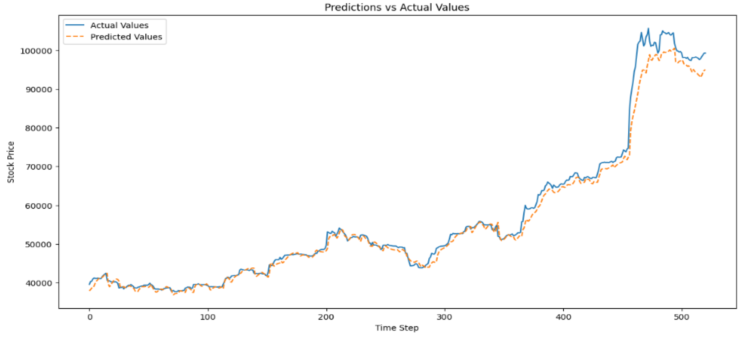
Figure 12.
Plot Actual vs. Predicted NGX Price Values on LSTM Model.
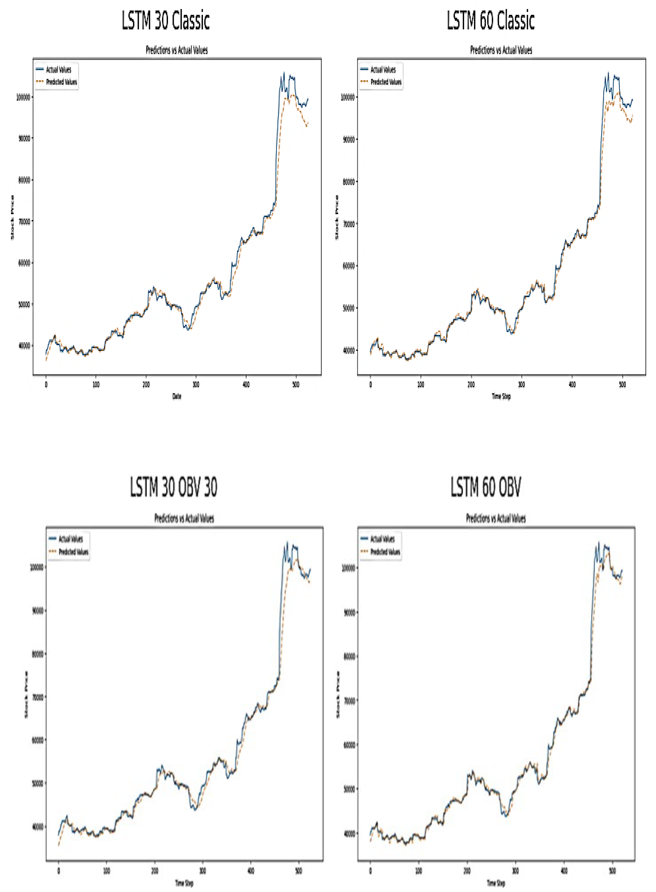
The plot below shows the actual (blue line) vs. predicted values (orange line) from an LSTM model applied to NGX market data. The x-axis shows the data point which represents individual samples, while the y-axis is the value of the target variable i.e. predicted NGX market price.
The provided plots above shows the actual versus predicted values of NGX price index using LSTM models with classic and OBV inclusion approach of a 30 and 60 day time-step. Each plot shows the performance and value of LSTM model for predicting NGX price movement. The observation shows that the predicted plots of classic 30 and 60days time steps track the actual NGX price closely from the beginning until towards the end of the plots when significant rise in NGX price occurs. At those time-steps, the model seems to lag behind the actual values. The 60-day model appears to follow the actual NGX price with slightly more accuracy and less delay than the 30-day model. The high accuracy of the classic 60-day model in tracking the actual NGX value suggest that longer time-steps capture more relevant temporal dependencies for predicting NGX price movements, most especially in capturing the upward trends. Furthermore, the observation of OBV inclusion plots appears to improve the predictive capability of LSTM. This is seen towards the end of the 60 days OBV inclusion plot where the actual NGX values are closer to the actual values during rapid price changes. OBV includes volume trends and this is essential during periods of significant price changes. It shows stronger buying or selling pressure and this is also evident from classic approach. All the four plots show some degree of discrepancies (lag) behind the actual NGX values during period of rapid and peak price changes. The lag could be due to the reactive nature of the input features and LSTM model inherent characteristics, where past data influences the prediction more strongly than sudden changes. Although, the addition of OBV seems to reduce this discrepancy slightly, which shows volume data provides essential information during market volatility. The lag areas show potential areas where the model prediction could be improved on or require additional feature engineering.
Diagnostic Evaluation
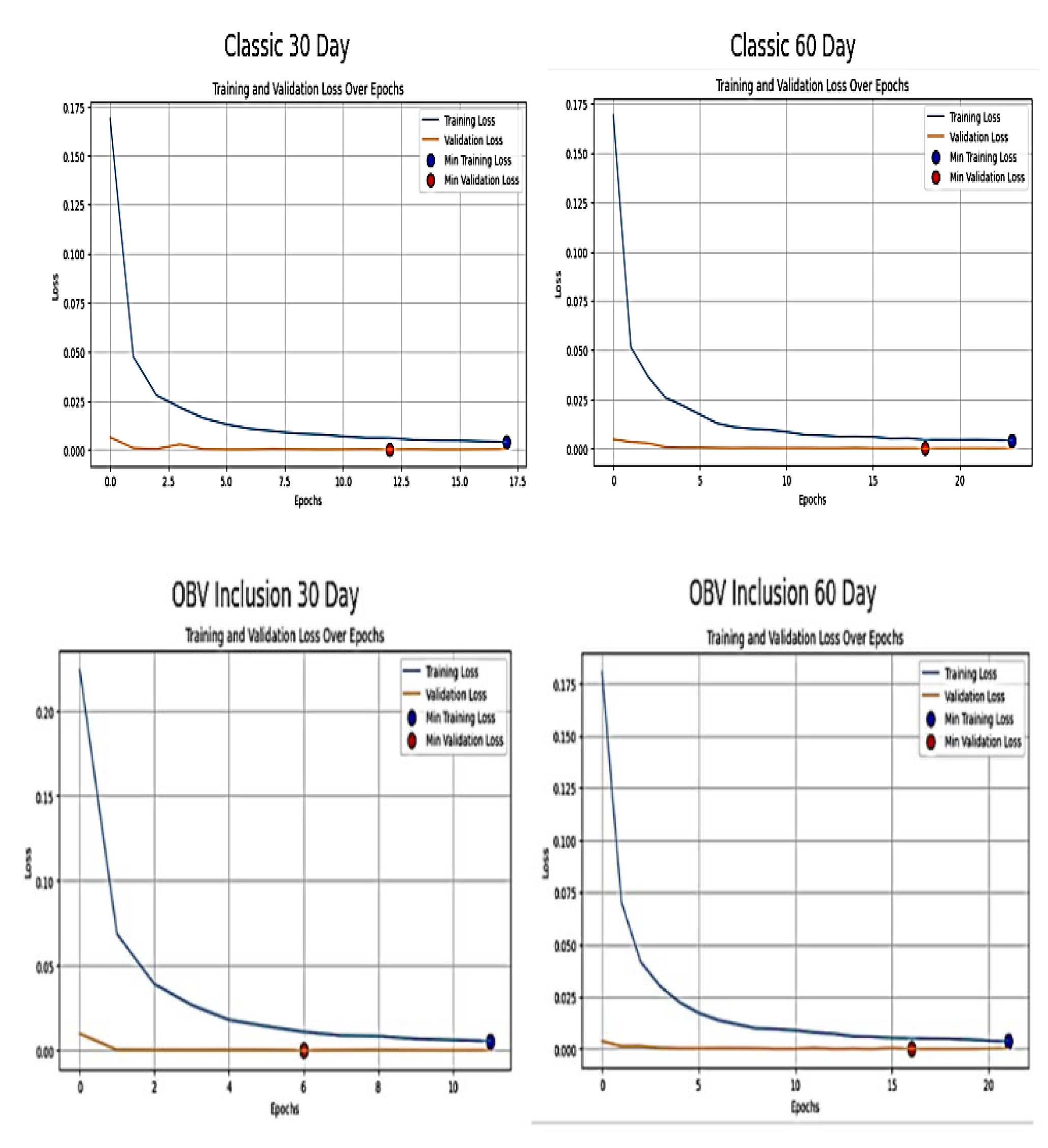
Further diagnostic tool such as the training and validation loss over epoch was employed to visually represent the model learning process. It assists in identifying overfitting and underfitting, comprehending model behaviour and making well informed judgements that enhance model performance [37]. The learning curve below showed X-axis as the epochs (training iterations) and Y-axis as the loss (error)
Figure 12.
Learning curve of the developed LSTM Model.
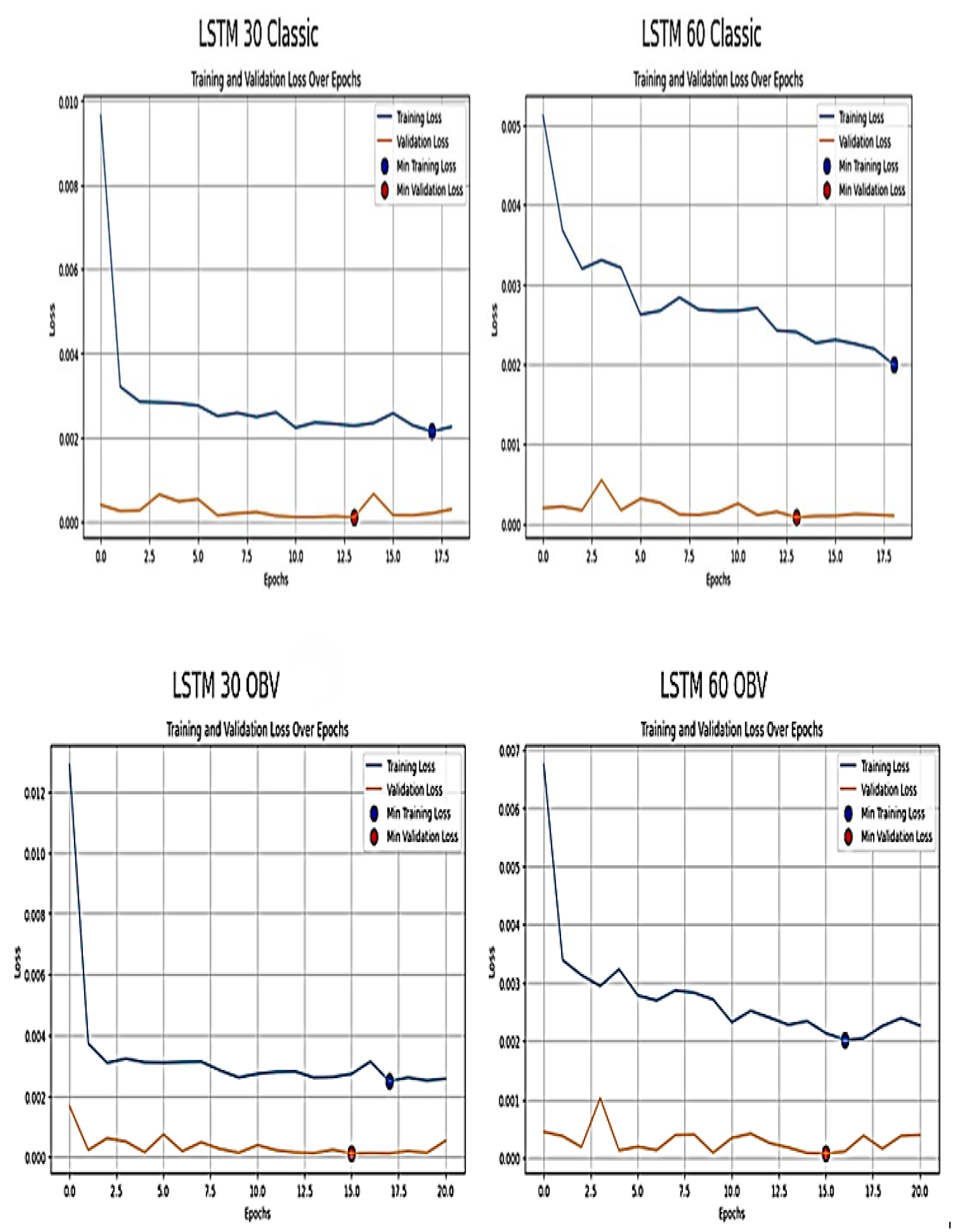
The classic LSTM 30 days exhibit initial rapid loss to a minimum loss of 0.002163, while the classic LSTM 60days model show more consistent decrease in training loss to a minimum loss of 0.001993 as epoch increases. This suggests the models generalises better as time-step increases and the stable loss in longer time steps assist in capturing more relevant market underlying information and trends. The plots show close convergence of validation and training loss, indicating good generalization without overfitting. However, the inclusion of OBV increases initial training loss values, which is obvious in the LSTM 30 OBV but steadily follow downward trend to a minimum training loss of 0.002493 and 0.002028 in LSTM 60 OBV. This implies that OBV adds complexity due to its sensitivity to volume changes. Despite this, LSTM models continue to learn well and leverage OBV for improved predictive accuracy. The LSTM 60 OBV inclusion also demonstrates it can handle more complexity introduced by OBV and this is shown by a more steady reduction in validation loss to a minimum of 0.000076. This confirms that longer sequences might help LSTM model to use the additional information provided by OBV more effectively. However, the consistent reduction in loss suggests that with sufficient training, these models are capable of leveraging OBV for improved predictive accuracy.
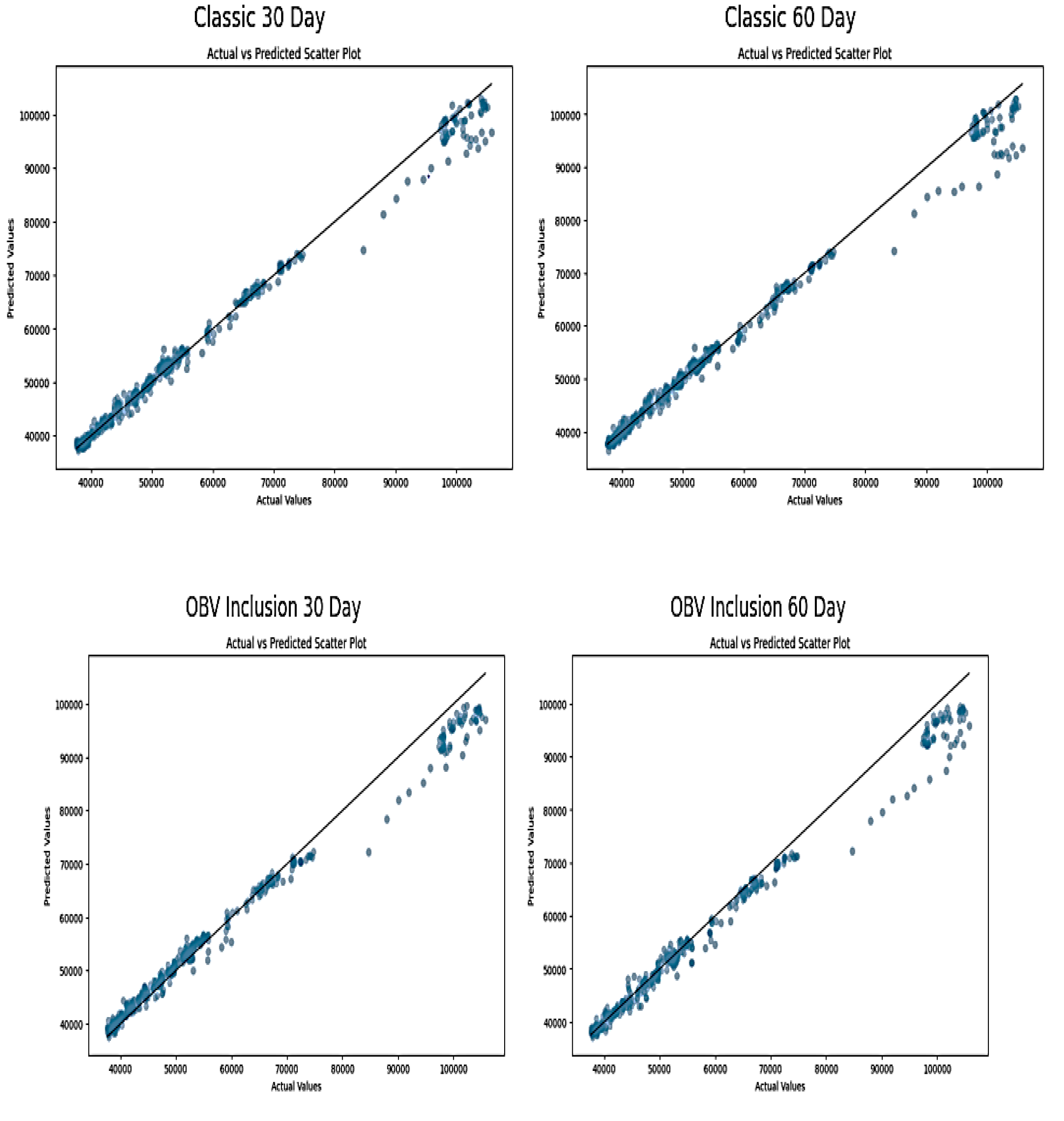
Figure 13.
Scatter Plots of Actual versus Predicted NGX price on LSTM Model.
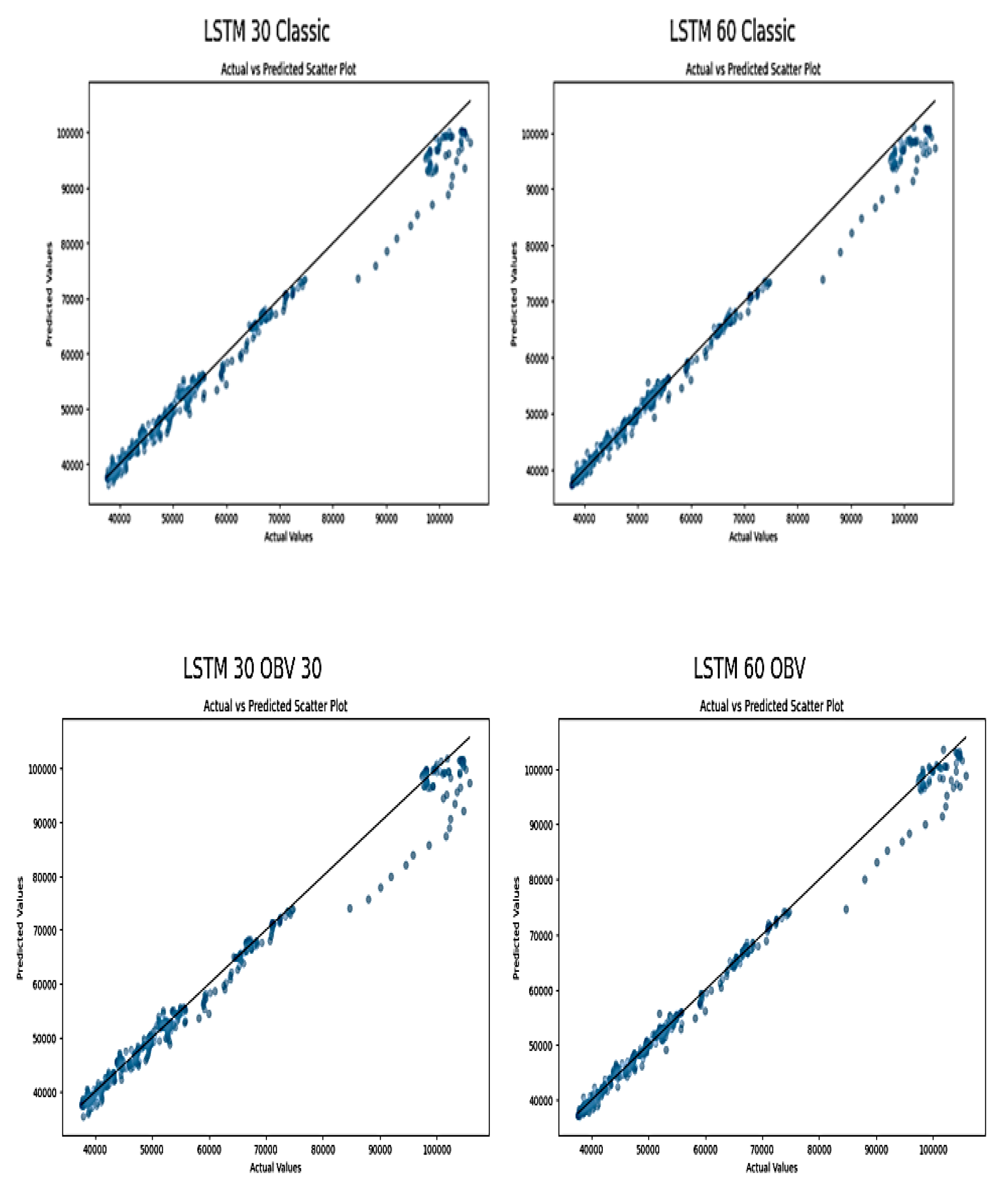
The scatter plots showed below illustrates the relationship between actual and predicted stock NGX prices by LSTM models
The LSTM 30 Classic and LSTM 60 Classic show a linear relationship between actual and predicted values, which indicates effective learning. However, LSTM 60 Classic plot is more tightly clustered around the diagonal. This indicates higher accuracy and better prediction consistency compared to the LSTM 30 Classic. It affirms that using longer time steps (60 days) can captures more relevant temporal patterns in the data, which will improve prediction accuracy. Also, the OBV inclusion plots points more closely aligning with the diagonal and this improves prediction of scatter distribution in both the 30-day and 60-day set up. Although, the LSTM 60 OBV model displays a very tight cluster around the diagonal, which demonstrates effective match between predicted and actual values. This is due to the combined effect of longer sequence learning and the inclusion of volume data that provides additional market sentiment insights.
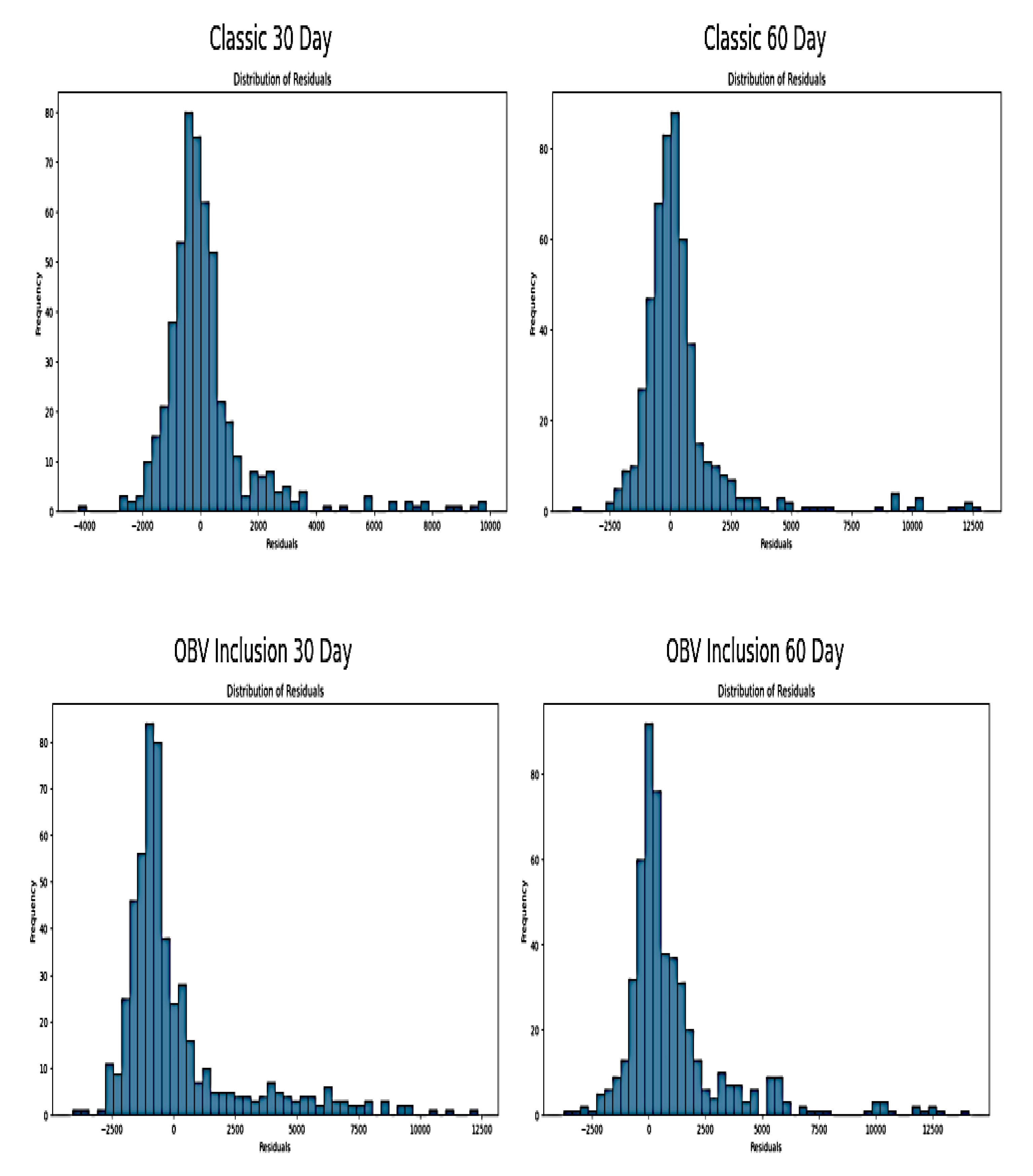
The residual plots below shows the frequency distribution of residuals from LSTM models trained on NGX market data and it compares the set up with 30 and 60-day time step on classic and with inclusion of OBV approaches.
Figure 14.
Residual Plots of LSTM.
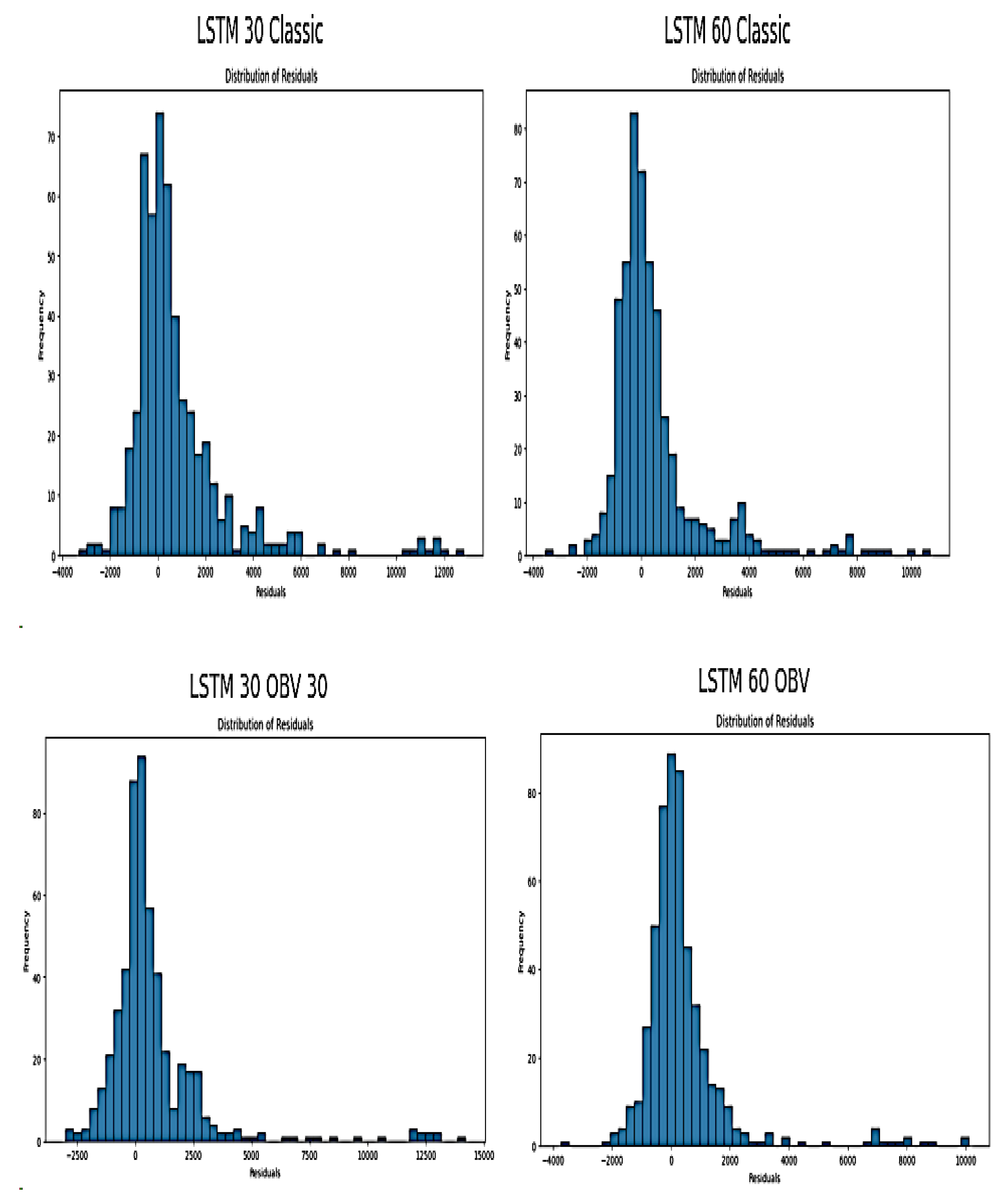
The distribution of classic LSTM 30 and LSTM 60-day time step are centered around zero. This is a good fit and it suggests that there is no systematic bias in the prediction. However, the classic LSTM 30 shows a broader spread of residuals compared to classic LSTM 60 which are more concentrated distribution. A more tight distribution of the classic LSTM 60 shows better prediction accuracy and model stability over medium to long term time-steps as it captures more relevant market dynamics. However, the plots of the second approach that include OBV show a widespread residuals and this specify that OBV introduces additional complexity into the LSTM predictions. There is a slight right skew in all models with tails, and is more visible in the 30-day models. This implies that the models might be under-predicting occasionally than over-predicting. This skewness is common in financial market prediction because of the extreme values that occur often than what a normal distribution would predict.
5. Conclusions
This study compared the performance of SVR, RNN, and LSTM models in predicting NGX market prices. While SVR demonstrated strong performance with smaller datasets and simpler market conditions, it struggled to capture the complex temporal dependencies in stock price data. RNN, although designed to handle sequential data, showed limitations due to the vanishing gradient problem, resulting in lower predictive accuracy over long periods. LSTM emerged as the most effective model for stock price prediction in this study. Its ability to retain information over long time sequences allowed it to outperform both SVR and RNN, most especially when dealing with volatile and unpredictable market trends. The results demonstrated that LSTM achieved the lowest error results and the highest R-squared values, highlighting its superior ability to capture both short-term and long-term dependencies in stock market data.
The research findings suggest that while SVR can be a useful tool for simple financial forecasting, LSTM provides far more accurate predictions for time-series data, particularly in complex and volatile markets. The integration of exogenous data, such as financial news sentiment, could further enhance the accuracy of deep learning models, offering valuable insights for investors and financial analysts
Author Contributions
Conceptualization, S.A and O.S.; methodology, S.A. and O.S; software, S.A. and O.S.; validation, O.S., O.P., and O.O.; formal analysis, S.A. and O.S.; investigation, S.A. and O.S.; resources, O.S.; data curation, S.A.; writing—original draft preparation, S.A..; writing—review and editing, O.S., O.P. and O.O.; supervision, O.S.; project administration, O.P., O.O. and O.S.; All authors have read and agreed to the published version of the manuscript
Funding
This research received no external funding.
Institutional Review Board Statement
Not applicable
Informed Consent Statement
Not Applicable.
Data Availability Statement
Data is available upon request
Conflicts of Interest
The authors declare no conflicts of interest.
References
- Han H, Liu Z, Barrios Barrios M, Li J, Zeng Z, Sarhan N, Awwad EM. Time series forecasting model for non-stationary series pattern extraction using deep learning and GARCH modeling. Journal of Cloud Computing. 2024 Jan 2;13(1):2.
- Abuein QQ, Shatnawi MQ, Aljawarneh EY, Manasrah A. Time Series Forecasting Model for the Stock Market using LSTM and SVR. International Journal of Advances in Soft Computing & Its Applications. 2024 Mar 1;16(1).
- Zulfiker MS, Basak S. Stock Market Prediction: A Time Series Analysis. ResearchGate. 2021. Available from: https://www.researchgate.net/publication/354362969.
- Lakshminarayanan SK, McCrae JP. A Comparative Study of SVM and LSTM Deep Learning Algorithms for Stock Market Prediction. CEUR Workshop Proceedings. 2019. Available from: https://ceur-ws.org/Vol-2563/aics_41.pdf.
- Pashankar SS, Shendage JD. Machine Learning Techniques For Stock Price Prediction-A Comparative Analysis Of Linear Regression, Random Forest, And SVR. Journal of Advanced Research in Computer Science. 2024. Available from: https://search.ebscohost.com/login.aspx?AN=175815713.
- Li X, Liang C, Ma F. Forecasting Stock Market Volatility with a Large Number of Predictors: New evidence from the MS-MIDAS-LASSO model. Ann Oper Res. 2022;1-40.
- Dong X, Li Y, Rapach DE, Zhou G. Anomalies and the expected market return. J Finance. 2022;77(1):639-681.
- Sarainmaa O. Swing Trading the S&P500 Index with Technical Analysis and Machine Learning Methods with Responsible Way [dissertation on the internet]. Abo Akademi University; 2024. Available from: https://www.doria.fi/handle/10024/189661.
- Badhe T, Borde J, Thakur V, Waghmare B, Chaudhari A. Comparison of different machine learning methods to detect fake news. In: Abraham A; et al., editors. Innovations in Bio-Inspired Computing and Applications. IBICA 2021. Lecture Notes in Networks and Systems. Cham: Springer; 2022. p. 419. Available from: . [CrossRef]
- Cormen, T. H., Leiserson, C. E., Rivest, R. L., & Stein, C. (2022). Introduction to Algorithms. MIT press.
- Edward, Suharjito. Tesla Stock Close Price Prediction Using KNNR, DTR, SVR, and RFR. J Hum Earth Futur. 2022;3(4):403–422. [CrossRef]
- Roy D, Sarkar T, Kamar S, Goswami T, Muktadir M, Al-Ghobari H. Daily Prediction and Multi-Step Forward Forecasting of Reference Evapotranspiration Using LSTM and Bi-LSTM Models. Agronomy. 2022;12(30594). Available from: . [CrossRef]
- Vikas K, Kotgire K, Reddy B, Teja A, Reddy H, Salvadi S. An Integrated Approach Towards Stock Price Prediction using LSTM Algorithm. 2022 International Conference on Edge Computing and Applications (ICECAA); 2022. p. 1696-1699. Available from: . [CrossRef]
- Benidis K, Rangapuram SS, Flunkert V, Wang Y, Maddix D, Turkmen C, Januschowski T. Deep learning for time series forecasting: Tutorial and literature survey. ACM Comput Surv. 2022;55(6):1-36.
- Mehmood, F., Ahmad, S., & Whangbo, T. K. (2023). An Efficient Optimization Technique for Training Deep Neural Networks. Mathematics, 11(6), 1360.
- Ghadimi, N., Akbarimajd, A., Shayeghi, H., & Abedinia, O. (2022). Improving time series forecasting using LSTM and attention models. Journal of Ambient Intelligence and Humanized Computing. [CrossRef]
- Espíritu Pera JA, Ibañez Diaz AO, García López YJ, Taquía Gutiérrez JA. Prediction of Peruvian companies' stock prices using machine learning. In: Proceedings of the First Australian International Conference on Industrial Engineering and Operations Management. Sydney, Australia: IEOM Society International; 2022. p. 20-21.
- Tawakuli A, Havers B, Gulisano V, Kaiser D. Survey: Time-series data preprocessing: A survey and an empirical analysis. J Eng. 2024. Available from: https://www.sciencedirect.com/science/article/pii/S2307187724000452.
- Ibrahim KSMH, Huang YF, Ahmed AN, Koo CH, El-Shafie A. A review of the hybrid artificial intelligence and optimization modelling of hydrological streamflow forecasting. Alexandria Eng J. 2022;61(1):279-303.
- López-González J, Peña D, Zamar R. Detecting and handling outliers in financial time series: Methods and applications. J Financ Econom. 2023;21(2):345-369.
- Zhu X, Zhang Y, Li X. The impact of non-stationarity on machine learning models in financial time series. Quant Financ. 2024;24(1):95-110.
- Lewis CD. Industrial and business forecasting methods: A practical guide to exponential smoothing and curve fitting. London; Boston: Butterworth Scientific; 1982.
- Song R, Shu M, Zhu W. The 2020 global stock market crash: Endogenous or exogenous? Physica A Stat Mech Appl. 2022;585:126425. Available from: . [CrossRef]
- Salem FM, Salem FM. Recurrent neural networks (RNN): From simple to gated architectures. Recurrent Neural Networks. 2022;43-67.
- Moodi F, Jahangard-Rafsanjani A, Zarifzadeh S. Feature selection and regression methods for stock price prediction using technical indicators. arXiv preprint arXiv:2310.09903. 2023. Available from: https://ui.adsabs.harvard.edu/abs/2023arXiv231009903M/abstract.
- Gupta A, Kapil D, Jain A, Negi HS. Using neural network for financial forecasting. In: Proceedings of the 2024 5th International Conference for Emerging Technology (INCET). IEEE; 2024. p. 1-6.
- Zhao X, Chung HM. Enhancing financial forecasting models with technical indicators. J Financ Data Sci. 2023.
- Swamy SR, Rajgoli SR; et al. Stock market prediction with machine learning: A comprehensive review. Indiana J Multidiscip Res. 2024. Available from: . [CrossRef]
- Zhang Y, Zhong W, Li Y, Wen L. A deep learning prediction model of DenseNet-LSTM for concrete gravity dam deformation based on feature selection. Eng Struct. 2023;295:116827.
- Mba JC. Assessing portfolio vulnerability to systemic risk: A vine copula and APARCH-DCC approach. Financ Innov. 2024;10(1):20. Available from: . [CrossRef]
- Janardhan N, Kumaresh N. Enhancing the early prediction of depression among adolescent students using dynamic ensemble selection of classifiers approach based on speech recordings. Int J Early Child Spec Educ. 2022;14(Spl Issue 02). Available from: .
- Lønning K, Caan MW, Nowee ME, Sonke JJ. Dynamic recurrent inference machines for accelerated MRI-guided radiotherapy of the liver. Comput Med Imaging Graph. 2024;113:102348. Available from: . [CrossRef]
- Muralidhar KSV. Demystifying R-Squared and Adjusted R-Squared. Built In. 2023. Available from: https://builtin.com/data-science/adjusted-r-squared.
- Liu Y. Stock prediction using LSTM and GRU. In: 2022 6th Annual International Conference on Data Science and Business Analytics (ICDSBA). IEEE; 2022. p. 1-6. Available from: .
- Gheisari M, Ebrahimzadeh F, Rahimi M, Moazzamigodarzi M, Liu Y, Dutta Pramanik PK, Kosari S. Deep learning: Applications, architectures, models, tools, and frameworks: A comprehensive survey. CAAI Trans Intell Technol. 2023;8(3):581-606.
- Zhou F, Wang Y. Enhancing stock market prediction with LSTM models incorporating volume indicators. J Financ Data Sci. 2023.
- Mohr F, van Rijn JN. Learning curves for decision making in supervised machine learning: A survey. arXiv preprint arXiv:2201.12150. 2022. Available from: . [CrossRef]
- Li C, Song Y. Applying LSTM model to predict the Japanese stock market with multivariate data. J Comput. 2024;35(3):27-38.
- Dhafer AH, Mat Nor F, Alkawsi G, Al-Othmani AZ, Ridzwan Shah N, Alshanbari HM, Baashar Y. Empirical analysis for stock price prediction using NARX model with exogenous technical indicators. Comput Intell Neurosci. 2022;202.
- Poernamawatie F, Susipta IN, Winarno D. Sharia Bank of Indonesia stock price prediction using long short-term memory. J Econ Financ Manag Sci (JEFMS). 2024;7(07):4777. Available from: .
- Jang D, Lee B. When machine learning meets social science: A comparative study of ordinary least square, stochastic gradient descent, and support vector regression for exploring the determinants of behavioral intentions to tuberculosis screening. Asian Commun Res. 2022;19(3):101-118.
- Huang H, Wei X, Zhou Y. An overview on twin support vector regression. Neurocomputing. 2022;490:80-92. Available from: . [CrossRef]
- Huang AH, Wang H, Yang Y. FinBERT: A large language model for extracting information from financial text. Contemp Account Res. 2023;40(2):806-841.
- Kim SI, Noh Y, Kang YJ, Park S, Lee JW, Chin SW. Hybrid data-scaling method for fault classification of compressors. Measurement. 2022;201:111619.
- Bathla G. Stock price prediction using LSTM and SVR. In: 2020 Sixth International Conference on Parallel, Distributed and Grid Computing (PDGC). IEEE; 2020. p. 211-214.
- Patel J, Shah S, Thakkar P, Kotecha K. A predictive model for stock price prediction using LSTM. Prod Plan Control. 2022;33(2):217-232. Available from: Taylor & Francis.
Disclaimer/Publisher’s Note: The statements, opinions and data contained in all publications are solely those of the individual author(s) and contributor(s) and not of MDPI and/or the editor(s). MDPI and/or the editor(s) disclaim responsibility for any injury to people or property resulting from any ideas, methods, instructions or products referred to in the content. |
© 2024 by the authors. Licensee MDPI, Basel, Switzerland. This article is an open access article distributed under the terms and conditions of the Creative Commons Attribution (CC BY) license (http://creativecommons.org/licenses/by/4.0/).
Copyright: This open access article is published under a Creative Commons CC BY 4.0 license, which permit the free download, distribution, and reuse, provided that the author and preprint are cited in any reuse.


