
Submitted:
02 May 2024
Posted:
06 May 2024
You are already at the latest version
Abstract
Longitudinal cutting is a most common process in steel structure manufacturing, and the man-hours of the process provide an important basis for enterprises to generate production schedules.However, currently the man-hours in factories are mainly estimated by experts, and the accuracy of this method is relatively low.In this study,we propose a system that predicts man-hours with history data in the manufacturing process and that can be applied in practical structural steel fabrication.The system addresses the data inconsistency problem by one-hot encoding and data normalization techniques,Pearson correlation coefficient for feature selection,and the Random Forest Regression(RFR) for prediction.Compared with the other three Machine Learning(ML) algorithms, the Random Forest algorithm has the best performance.The results demonstrate that the proposed system outperforms the conventional approach and has better forecast accuracy, so that it is suitable for man-hours prediction.
Keywords:
Man-hour prediction
; RFR
; steel fabrication
; ML
; predictive system
1. Introduction
The production planning and scheduling of steel structure manufacturing enterprises is an important task, and the processing time of components is an important reference for enterprises to arrange overall production plans and determine production nodes for components. The accuracy of man-hour prediction greatly affects production planning and full process scheduling of enterprises.Taking the longitudinal cutting steel coil processing of steel structure manufacturing enterprises as an example, the man-hour of processing generally includes dozens of process times,such as loading time, tailing time, unloading time, separation plate replacement time, material return time, slitting tailing time, etc. The current workshop scheduling mainly revolves around processing time, and is based on the premise of determined processing time. That is, the same components and processing procedures are processed using the same model of machine, and the processing time remains unchanged.However, in the actual production process, due to the influence of worker proficiency, workshop environment, lighting, and physical parameters of steel in the process flow, the cutting process of steel coils is greatly affected by factors such as raw material specifications,width, and thickness of the workpieces, resulting in an uncontrollable fluctuation in production hours, which leads to a certain deviation between the used processing hours and the actual processing hours. With the continuous progress of production and the accumulation of man-hour deviations, the production plan executed on the production line deviates from the pre-arranged production plan. This estimation of production tasks and operation time based on inaccurate man-hours parameters can lead to significant deviations between plan and actual production, which can easily lead to implementation gaps[1,2].Even through rescheduling and resource rearrangement, it is difficult to compensate for the impact of man-hour deviations. Moreover, rescheduling and resource rearrangement consume a lot of manpower and time, thereby reducing the feasibility of the entire production plan, which makes it difficult for production plans to effectively guide the actual production operations of enterprises.
At present, the prediction of the man-hours is carried out by an expert based on the historical production data in most structural steel fabrication enterprises. The expert uses various factors to predict the man-hours, but such process carries the some problems:
- First of all, and most importantly, the prediction is not objective. A human ultimately carries out the expert prediction, and therefore there is no guarantee of a consistent prediction. Further, there is the concern that factors that are difficult to objectify may lower the accuracy of predictions[3].
- There is a complex relationship between man-hour and these subjective factors, where significant amount of effort and time are required to make predictions.
- It is difficult to share the implicit know-hows of experts over prediction, and these know-hows are also difficult to quantify. Therefore any person other than the applicable expert needs to assign significant prior experience.
Such problems could be overcome by using the man-hour prediction model.In manufacturing production, the man-hour parameter is an important basis for production planning and scheduling[4],and is used to determine the amount of work tasks and the time interval for each task,which is a key parameter in planned production.Some related studies in recent years, such as data-based scheduling models[5] and data-based methods for predicting key parameters[6] have proved that mining relevant information and knowledge from underlying data and applying it to production decisions can reduce uncertainty in decision-making, enable rapid analysis, and reduce the number of erroneous decisions[7]. If the factors that affect man-hours are identified and quantified, and a prediction model is established based on these factors, then a low-cost, objective and efficient prediction can be performed.
The remainder of the article is organized as follows: In section “Related works”, theoretical background related to predict man-hours and applications of Random Forest(RF) in different industries are analyzed.The data used in this study are discussed in “Data descriptions and preprocessing” section,and the method of data preprocessing such as data normalization ,one hot encoding and variable selection is also discussed.The man-hour prediction system suggested in this study is described in section “Models”. Section “Results and discussion” discusses the prediction model and its performance. Finally, in section “Conclusion” provides the significance and the limitations of this study.
2. Related Works
In recent years, thanks to widespread adoption such as big data, artificial intelligence, the Internet of Things,and general information technology infrastructure in manufacturing, scholars have conducted extensive research on the application of these technologies to man-hour prediction.Hur et al.[3] constructed a man-hour prediction system based on multiple linear regression and classification regression tree for the shipbuilding industry, and the results showed that the prediction system has strong reliability. Based on this study, three types of plans have been established in man-hour prediction, they are quarter plan, month plan and day plan respectively.YU et al.[8] conducted a study on the ML-based quantitative prediction of the process’ man-hour during aircraft’s assembly.The study proposed a forecasting model based on Support Vector Machine(SVM), which was optimized by particle swarm optimization.The authors showed that the improved model could effectively predict man-hour of assembly work in a short time while maintaining sufficient accuracy.Mohsenijam et al.[9] proposed a framework for labour-hour prediction in structural steel fabrication.The research explored a data-driven approach which used Multiple Linear Regression (MLR) and available historical data from Building Information Models (BIM) to associate project labour-hours and project design features.IşıkS et al.[10] explored the use of machine-learning techniques such as Support Vector Regression(SVR),Gaussian Process Regression(GPR) and Adaptive Neuro-Fuzzy Inference System(ANFIS) for predicting man-hours in Power Transformer manufacturing. The authors reported that these techniques,especially GPR are useful in the prediction of man-hours in Power Transformer production industry. The results showed that the predictive model based on GPR attained good performance in terms of effectiveness and usability and could be effectively used in an acceptable error range, especially when compared to pure expert forecast.Aiming at a kind of key equipment in the metal machining and weld machining, namely the multi-station and multi-fixture machining center.DONG et al.[11] designed a man-hour calculation system for a motorcar manufacturing company, which was based on .the practical production situation, manual time and parallel time between man and machine.Hu[12] proposed a man-hour prediction model based on optimizing back propagation neural network with genetic algorithm (AG_BP) for the management process of chemical equipment design.The results showed that the model could be a good solution for predicting man-hours required for chemical equipment design and improve the prediction accuracy.
In recent years, there has been a growing interest in using ML algorithms to solve both linear and non linear problem in regression analysis.The RF algorithm,as an ensemble learning algorithm based on CART decision trees, is widely used in classification or regression problems[13,14].Fraiwan et al.[15] proposed an automated sleep stage identification system based on time-frequency analysis of a single EEG channel and a RF classifier. The results demonstrate that the system achieves an accuracy of 83% in classifying the five sleep stages.Yanni Dong[16] proposed an efficient metric learning detector based on RF, which was applied to the classification of HSI data. Experimental results demonstrated that the proposed method outperformed state-of-the-art target detection algorithms and other classical metric learning methods.Berecibar et al.[17] presented a novel machine learning approach for online battery capacity estimation. By establishing a RFR model to approximate the relationships between features, it accurately estimated the capacity of aged batteries under various cycling conditions.Liu et al.[18] proposed a classification framework utilizing RF, integrating Out-of-Bag(OOB) prediction,Gini variation,and Predictive Measure of Association (PMOA).The approach aimed to accurately evaluate the significance and correlation of battery manufacturing features and their influence on the classification of electrode properties.Tarchoune et al.[19] proposed a hybrid model named 3FS-CBR-IRF (Three feature selection - Case based reasoning - Improved random forest) to apply for the evaluation of medical databases. The model was evaluated on 13 medical databases, and the results indicated an improvement in the performance of the CBR system. Li et al.[20] utilized a GIS platform to assess the sensitivity of slope-type geological hazards in the study area using the information value model and the RF weighted information value model. The approach addressed the issue of negative impacts caused by sensitivity zoning results. The results indicated that the proposed models exhibited high ROC accuracy.Moin Uddin et al.[21] presented a novel hybrid framework combining feature selection, oversampling,and hybrid RF classifier to predict the adoption of vehicle insurance.The framework could benefit insurance companies by reducing their financial risk and helping them reach out to potential customers who are likely to take vehicle insurance.
With this backdrop,the above studies show that ML algorithms and data-mining techniques have been wildly used in the man-hours prediction and a variety of industries.However different ML algorithms have different advantages and disadvantages, the algorithms suitable for different specific fields are also different.Different specific requirements require different algorithms or the integration of multiple technologies to improve the accuracy and stability of the model.
On the basis of extensive study of man-hour prediction methods and the present project-based production environments, we listed various related variables. Then we utilized Pearson correlation coefficient to perform variable selection to identify the essential features for enhancing accuracy. A prediction system based on RFR model was developed in this study for the prediction of the man-hour. More over, the predictive performance was also compared with three other machine learning models.
3. Data Descriptions and Preprocessing
3.1. Data Descriptions
To build the man-hour prediction system,we collected processing data from the production lines of a steel structure enterprise for a total of two years, including 2022, and 2023.There are over 5000 rows of data in this dataset, each with 11 attributes. Two of these attributes (production schedule number and production bundle number) are attributes that uniquely represent the data and the other one is a textual description of the data.These three attributes are not relevant to the man-hour prediction,so we directly removed them prior to data preprocessing.One of the remaining nine attributes is the man-hour, which is the dependent variable to be predicted, and the remaining 7 attributes are independent variables.Attributes are mostly of numeric and character types.Table 1 shows further specific descriptions for the dataset.
3.2. Data Preprocessing
Data preprocessing is important to improve usability and accuracy for the model. For a given dataset, certain missing, unusual and redundant values were found after exploring all the data by analyzing and visualizing the distribution of each variable.This type of data cannot be directly used for model training, or the training results are unsatisfactory. In order to improve the accuracy of model predictions, data preprocessing techniques have emerged. There are various methods for data preprocessing: data cleaning, data integration, data transformation, data normalization, etc. These data processing techniques used before machine learning can greatly improve the quality of model predictions and reduce the time required to train the model.
In the steel structure manufacturing enterprise we cooperate with, each steel plate to be processed would be labeled with a QR code, which would be scanned to record the starting time of steel plate processing when the workers fed the plate into the machine for processing, and then scanned again to record the end time of processing after the end of processing, so that the actual processing time could be calculated through the processing starting time and the end time.However, in the actual operation process, workers might forget to scan the code at the beginning or end of processing, and instead scaned and recorded the time after a certain period of processing, thus resulting in a significant error between the actual processing time and the processing time recorded by the scan.This kind of data that deviates significantly from the actual real data is called noise. Noise can cause deviations in the prediction model, which seriously affects the accuracy of the model, so it is necessary to remove the noisy data before modeling.After analysis, it was found that workers forgetting to scan the code would result in either a very small or very large recorded processing time values.In response to this situation, this paper adopts an outlier detection based on box graph method to remove nearly 2000 noisy data.Finally,3000 pieces of data were left to form the dataset, which was divided in an 8-2 ratio,2400 pieces of data were placed in the training set, and 600 pieces of data were placed in the testing set.
For discrete data , such as business type (X4) is divided into two types: incoming material processing and delivery, this article uses one-hot encoding for conversion. One-hot encoding is a common method for converting character data into discrete integer encoding.After using one-hot encoding, 1 represents incoming processing and 0 represents incoming delivery. This can convert character features into numerical features that can be recognized by machine learning models.
The units of X1,X2....,X8 are different and the magnitude of them differs tremendously.For example, the unit of raw material weight is kilogram, while the unit of allocated length is meter, and data from different units cannot be compared. If the original data is directly used for model training, it will enhance the impact of features with larger numerical scales on the model, weaken or even ignore the effect of features with smaller numerical scales.Therefore, in order to significantly reduce the interference of features in terms of different value scales and ensure the effectiveness of the model training and fitting process, it is necessary to standardize the feature variables of the original sample data, so that the features of each dimension have the same weight impact on the model objective function.In this paper, equation(1) is used to min-max normalize the sample by scaling the range of values of each variable to between [0,1]. In equation (1), x* represents the normalized new value, xmin represents the minimum value of the sample, and xmax represents the maximum value of the sample.
3.3. Input Variable Selection
Minimizing the number of input variables significantly reduces the likelihood of over-fitting, collinearity (high correlation between input variables), and transferring noise from data to the calibrated model (Ivanescu et al. 2016)[22].Having too many input variables, the regression model tends to fit itself to the noise hidden in the training set instead of generalizing underlying patterns and hidden relationships. A proper method for variable selection removes those insignificant or redundant input variables from the regression model (Akinwande et al. 2015)[23].
In the field of natural sciences, the Pearson correlation coefficient is widely used to measure the degree of correlation between two variables. The Pearson correlation coefficient between two variables is defined as the quotient of the covariance and standard deviation between the two variables, as shown in equation (2),where cov(X,Y) represents the covariance between X and Y, δX represents the standard deviation of X, and E[X] represents the expected value of X.
For discrete random variables, the Pearson correlation coefficient is calculated as shown in equation (3).
Pearson correlation coefficient varies from -1 to 1. The value of the coefficient is 1, which means that X and Y can be well described by the linear equation, and all data points fall well on the same line, and Y increases with the increase of X.-1 means that all data points fall on a straight line, and Y decreases as X increases. 0 means that there is no linear relationship between the two variables.
This paper analyzed the Pearson correlation coefficients between man-hours(Y) and variables X1~X11 respectively, the results are demonstrated in Table 2. Pearson correlation coefficients bigger than 0.4 mean good correlation, bigger than 0.5 mean strong correlation and bigger than 0.6 represent very strong correlation.We selected variables with a correlation greater than 0.4 with man-hours (Y), which are raw material width(X2), allocated length (X5), allocated weight (X6), and finished product width (X8).
4. Models
4.1. Man-Hour Prediction System
In this study, a man-hour prediction system which consists of data preprocessing, input variable selection and model prediction was established. Data preprocessing and input variable selection have been discussed in detail above. After data preprocessing and input variable selection, a ML model is applied to forecast the target outputs. After training the ML model, separate predictions are conducted on test data to check the progress of the ML model.Figure 1 shows the overall work flow of the man-hour prediction system which includes data prepocessing and prediction.
Historical data is a comprehensive reflection of the internal mechanism of a system’s changes.The number of historical data shows the mechanism of the changes in an extent(Bing,2014)[24].We obtained historical processing data from the partner companies, and then used data cleaning methods to remove the noisy data;used one-hot coding to convert the text data into discrete data, and then normalized the data using min-max normalization;used Pearson correlation coefficient for variable selection, and then used machine learning regression models for man-hour prediction.
Machine learning is now widely used in man-hour prediction and workshop production, such as SVM[25],Back Propagation Neural Network(BPNN)[26],Decision Tree(DT)[27],etc.In order to obtain the optimal prediction results,this paper selected four models:SVM, BPNN, RF and Logistic Regression (LR)[28] for experiments.In order to obtain optimal model prediction performance,appropriate model parameters need to be used.For the above 4 models, we used network search methods to optimize the parameters of the four models and selected the best model parameters for model prediction.
4.2. Random Forest Regression
RF is a combination of decision tree classifiers such that each tree depends on the values of an independently sampled vector with the same distribution for all trees in the forest[29].
A RF consists of a set of decision trees h(X, θk) where X is an input vector, θk is an independent and identically distributed random vector. θk is generated for the k-th tree independently of the previous random vectors θ1 ,...,θk-1, but with the same distribution. The reason for introducing θk is to control the growth of each tree. After many decision trees have been generated, the most popular class is voted. The k-th tree which is grown by a training set and θk , is equivalent to generating a classifier h(X, θk). In this sense, given a set of classifiers h(X, θ1), h(X, θ2),..., h(X, θk), and with the training set randomly presented from the distribution of the random vector Y, X where X is the sample vector and Y is the correctly classified classification label vector, the margin function is defined by Equation (4).
where I(x) is the indicator function.The margin function measures the extent to which the number of votes X, Y for the right class exceeds the maximum vote for any other error class-the larger the value, the higher the confidence of the classification. The generalization error is given by Equation (5)[30]:
where X and Y represent the definition space of probability.
According to the law of large numbers[31], as the number of decision trees increases, all sequences θk and PE will converge to Equation (6), corresponding to the frequency converging to probability in the law of large numbers.It explains why random forests do not overfit with the increase of decision trees and have a limited generalization error value.
The working flow of the random forest algorithm is as follows(also illustrated in Figure 2):
Step1—The n sub-data sets D1,D2,…,Dn are randomly selected from the whole data set D.
Step2—A decision is generated for each sub-data, i.e. n decision trees are generated according to n sub-data sets, and a prediction result is obtained for every single decision tree.
Step3—The third step votes for each decision tree based on their prediction results, and then summarize the voting results.
Step4—Based on the summarized voting results, the algorithm selects the predicted result with the most votes as the final algorithm's prediction result.
5. Results and Discussion
5.1. Performance Evaluation Metrics
To assess models, we employed the root mean square error (RMSE), mean absolute percentage error(MAPE), population stability index(PSI) which were very widely used for assessment in prediction. The formula are as follows:
In formulas (7) and (8), n represents the number of evaluated samples, yi represents the true value of the samples, i.e. actual man-hour, and ŷi represents the predicted value of the samples, i.e. estimated man-hour. The closer RMSE and MAPE are to 0, the better the predictive performance of the model. In formula (9),represents the mean of the sample, the meanings of n and yi are the same as those in formula (7) and (8). The closer R2 is to 1, the better the model performance; the closer it is to 0, the worse the model performance. In formula (10),is the actual proportion of the sample within the partition boundaries, and is the predicted proportion of each partition sample in the test dataset. PSI is used to measure the difference in data distribution between test samples and modeling samples, and is a common indicator of model stability. It is generally believed that model stability is high when PSI is less than 0.1, average when PSI is between 0.1 and 0.25, and poor when PSI is greater than 0.25.
5.2. Comparative Analyses
In this paper, the steel cutting hours were predicted using four models, (SVR), BPNN, LR, RFR, respectively.A total of 600 datas were used in the test set for prediction, and the parameters of each model were optimized using network search.Finally, experimental comparisons are conducted on the four prediction schemes,and the four man-hours prediction schemes are shown in Table 5.
Figure 3 shows histograms comparing the performance of four models, where Figure (a) shows the histograms of RMSE, MAPE, and R2.Due to the significant difference in magnitude between PSI and the other three metrics, in order to better demonstrate the comparative relationship of PSI, a separate comparison is made in Figure (b).Table 5 and Figure 3 show that the RMSE, MAPE, R2, and PSI of the RFR model are superior to the other three models. The RMSE of RFR is 0.69 lower than SVR, 0.98 lower than BPNN, and 1.18 lower than LR; The R2 of RFR is 0.03 higher than SVR, 0.04 higher than BPNN, and 0.05 higher than LR, indicating that the predicted man-hours of the RFR model are closer to the actual man-hours and have the smallest error.For MAPE , RFR is 1.52% lower than SVR, 2.18% lower than BPNN, and 2.61% lower than LR, which indicates that the RFR model has the highest prediction accuracy.The PSI value of all four models are less than 0.1, indicating that the stability of all four models is high, among which the PSI value of the RFR model is significantly lower than that of the other three models by one order of magnitude, indicating that the RFR model has the highest stability.
Because PSI is a metric of model stability, in order to better analyze the stability of the RFR model, we divided the samples into 10 intervals. Table 6 shows the detailed data for each interval of the RFR model, where actual represents the number of real samples in the interval, predict represents the number of predicted samples in the interval, actual_rate represents the percentage of actual samples in the interval to the total sample, and predict_rate represents the percentage of predicted samples in the interval to the total sample.As can be seen from Table 6,except for the difference of 11 between the number of predicted samples and the actual number of samples in the 3rd interval, there is not much difference between the number of predicted samples and the actual number of samples in the other 9 intervals, such as interval 8 and interval 10, where the difference is only 2 samples. This indicates that the RFR model has high stability in the prediction of man-hours.
The prediction result of test set by RFR is shown in Figure 4.The RFR model exhibited outstanding performance on the test set, achieving a coefficient of determination (R2) as high as 0.9447. This metric signifies the model's capability to elucidate the variability in the target variable. The R2 value of the RFR model underscores its considerable advantage in capturing the intricate relationship among steel processing hours. Furthermore, there exists a robust linear correlation between the model predictions and the actual observations, underscoring the RFR model's high level of accuracy and reliability in predicting steel longitudinal cutting processing time.
In order to further validate the performance of the model, we also presented SVR,BPNN and LR to make predict experiment. The forecasting results are shown in Figure 5, Figure 6 and Figure 7. Figure 5 shows the prediction result by SVR.The R2 value of the SVR model stands at 0.9125, slightly lower than that of the RFR model but still within an acceptable range, indicating the effectiveness of SVR in addressing nonlinear problems. SVR efficiently captures the nonlinear features of the data by identifying the optimal hyperplane in the high-dimensional space. Despite its slightly inferior prediction accuracy compared to RFR, SVR's robustness in handling small samples or high-dimensional data suggests its potential applicability in specific contexts.
The forecasting result of BPNN can be seen in Figure 6.The R2 value of the BPNN model stands at 0.9043, indicating a certain degree of accuracy in modeling the nonlinear relationship between the steel processing time. BPNN, as a deep learning model, can learn complex data mapping relationships through training with the back-propagation algorithm. Despite the potential requirement for more tuning parameters and computational resources, the BPNN's robust capability in handling large-scale datasets should not be overlooked, particularly in scenarios where data features are rich and model complexity requirements are high.
Figure 7 shows the prediction result of LR.The LR model yields R2 value of 0.8914, representing the weakest performance among the four models. However, this does not diminish LR's practical value. As a linear model, LR remains effective in handling simple linear relationships or serving as a benchmark model. Its simplicity and interpretability render it a reliable choice in certain scenarios, particularly in studies with limited datasets or stringent requirements for model interpretability.
The relative error of the RFR model is depicted in Figure 8, showcasing an average relative error of -1.7956%. This indicates that the model's predicted values on the test set generally tend to be lower than the actual values, exhibiting a slight negative bias. This bias could stem from the model's inadequate comprehension or overfitting of specific data features during the training process. However, given the high R2 value of the RFR model, the influence of this bias on the overall prediction results may be constrained.
Table 7 assesses the comparison of the prediction results by RFR,SVR,BPNN and LR.After comparison, it is obvious that the prediction result of RFR is much better than the other three models. It proves that RFR can be effectively applied to the prediction problem of man-hours while maintaining sufficient accuracy.
In summary, the findings of this study reveal that the RFR model exhibits the most effective performance in predicting steel longitudinal cutting processing time, followed by the SVR, BPNN, and LR models. These results offer a valuable tool for enhancing production optimization within the steel processing industry, with potential benefits including increased productivity and cost reduction. Future research endeavors could delve into optimizing model strategies, such as employing feature selection and dimensionality reduction techniques to enhance prediction accuracy. Additionally, integrating learning methods could combine the strengths of various models, thereby further improving prediction accuracy and robustness.
6. Conclusions
In the field of steel structure manufacturing, man-hour prediction has always been an indispensable part of production planning and scheduling. Accurate man-hour prediction is not only related to the production efficiency of enterprises, but also a key factor affecting the overall production process arrangement and cost control. This article proposes a man-hour prediction system based on historical data, focusing on this core issue, and elaborates on the key technologies of the system in data processing, feature selection, and prediction model construction.
In response to the issue of data inconsistency in the manufacturing process, this article adopted one-hot coding and data normalization techniques. These technologies not only solved the problem of diversity in data formats, but also improved the comparability of data and the stability of models. Through this step, we successfully transformed the raw data into effective inputs that the model can recognize.Pearson correlation coefficient was used to filter out features highly correlated with man-hours. This step not only reduced the complexity of the model and improved computational efficiency, but also identified the factors that have a decisive impact on man-hour prediction.After comparing multiple machine learning algorithms, the random forest regression algorithm was chosen as the main prediction model.Through training and optimization, the model showed superior performance in predicting man-hours.
The man-hour prediction system proposed in this article has higher prediction accuracy and stronger practicality compared to traditional expert estimation methods. The introduction of this system not only improves the accuracy of production planning and scheduling for enterprises, but also provides strong support for production cost control and efficiency improvement. The system has good scalability and flexibility. With the continuous accumulation of data in the manufacturing process and the emergence of new technologies, the system can be continuously optimized and upgraded to further improve the accuracy and efficiency of prediction. Meanwhile, the system can also be easily applied to other similar manufacturing fields, providing a solution for predicting man-hours for a wider range of production scenarios.
However, we must also recognize that any predictive model has its limitations and uncertainties. Although the system proposed in this article has greatly improved the accuracy of man-hour prediction, it may still be affected by some uncontrollable factors in practical applications, such as equipment failures, human operation errors, etc. Therefore, when using this system, we need to consider the actual situation comprehensively and make timely adjustments and optimizations.In the future, we will consider more factors, such as the proficiency of workers, the failure rate of machines, etc., in order to provide more efficient and accurate man-hour prediction services for enterprises.
Author Contributions
Conceptualization, Z.W. and Z.L.; methodology, Z.W. and P.L.; software, Z.W. and R.N.; validation, R.N., P.J. ; formal analysis, Z.Y.; investigation, Z.W. and Z.Y.; resources, Z.W. and Z.L.; data curation, Z.W. and Z.Y.; writing—original draft preparation, Z.W.; writing—review and editing, Z.L.; visualization, P.J. and Z.Y.; supervision, Z.L.; project administration, Z.L.; funding acquisition, Z.L. All authors have read and agreed to the published version of the manuscript.”
Funding
This research was funded by the National Natural Science Foundation of China (NSFC),grant number 62262057,the Innovative Development Project of Shihezi University,grant number CXFZ202101 and the Research Project of Shihezi University, grant number ZZZC202112.
Data Availability Statement
Not applicable.
Conflicts of Interest
The authors declare no conflict of interest.
References
- Li, L.; Zijin, S.; Jiacheng, N.; Fei, Q. Data-based scheduling framework and adaptive dispatching rule of complex manufacturing systems. Int. J. Adv. Manuf. Technol. 2013, 66, 1891–1905. [Google Scholar] [CrossRef]
- Li, Q.; Wang, L.; Xu, J. Production data analytics for production scheduling. In Proceedings of the 2015 IEEE International Conference on Industrial Engineering and Engineering Management, Washington, DC, USA; IEEE, 2015; pp. 1203–1207. [Google Scholar]
- Hur, M.; Lee, S.-K.; Kim, B.; Cho, S.; Lee, D.; Lee, D. A study on the man-hour prediction system for shipbuilding. J. Intell. Manuf. 2015, 26, 1267–1279. [Google Scholar] [CrossRef]
- Wu, X.; Zhu, X.; Wu, G.; Ding, W. Data mining with big data. IEEE Trans. Knowl. Data Eng. 2014, 26, 97–107. [Google Scholar]
- Liu, M.; Hao, J.H.; Wu, C. A prediction based iterative decomposition algorithm for scheduling large-scale job shops. Math. Comput. Model. 2008, 47, 411–421. [Google Scholar] [CrossRef]
- Gradisar, D.; Music, G. Production-process modelling based on production-management data:a Petri-net approach. Int. J. Comput. Integr. Manuf. 2007, 20, 794–810. [Google Scholar] [CrossRef]
- Obitko, M.; Jirkovsky, V.; Bezdicek, J. Big data challenges in industrial automation. In Proceedings of the International Conference on Industrial Applications of Holonic and Multi-Agent Systems; Springer: Berlin, Germany, 2013; pp. 305–316. [Google Scholar]
- Yu, T.; Cai, H. The Prediction of the man-hour in aircraft assembly based on support vector machine particle swarm optimization. J. Aerosp. Technol. Manag. 2015, 7, 19–30. [Google Scholar] [CrossRef]
- Mohsenijam, A.; Lu, M. Framework for developing labour-hour prediction models from project design features: Case study in structural steel fabrication. Can. J. Civ. Eng. 2019, 46, 871–880. [Google Scholar] [CrossRef]
- Kamil IşıkS,Emre Alptekin.A benchmark comparison of Gaussian process regression, support vector machines, and ANFIS for man-hour prediction in power transformers manufacturing[C]//Knowledge-Based and Intelligent Information & Engineering Systems: Proceedings of the 26th International Conference KES2022. Procedia Computer Science 2022, 207, 2567–2577.
- Dong, Q.; Lu, J.; Kan, S. A study on man-hour calculation model for multi-station and multi-fixture machining center. Adv. Intell. Soft Comput. 2012, 149, 403–411. [Google Scholar]
- Hu, M. Optimizing back propagation neural network with genetic algorithm for man-hour prediction in chemical equipment design. Chem. Eng. Trans. 2018, 66, 877–882. [Google Scholar]
- Breiman, L. Random forests. Machine Learning 2001, 45, 5–32. [Google Scholar] [CrossRef]
- Rokach, L. Ensemble-based classifiers. Artif. Intell. Rev. 2010, 33, 1–39. [Google Scholar] [CrossRef]
- Fraiwan, L.; Lweesy, K.; Khasawneh, N.; Wenz, H.; Dickhaus, H. Automated sleep stage identification system based on time-frequency analysis of a single EEG channel and random forest classifier. Comput. Methods Programs Biomed. 2012, 108, 10–19. [Google Scholar] [CrossRef]
- Dong, Y.; Du, B.; Zhang, L. Target Detection Based on Random Forest Metric Learning. IEEE J. Sel. Top. Appl. Earth Obs. Remote Sens. 2015, 1830–1838. [Google Scholar] [CrossRef]
- Li, Y.; Zou, C.; Berecibar, M.; Nanini-Maury, E.; Chan, J.C.-W.; Bossche, P.v.D.; Van Mierlo, J.; Omar, N. Random forest regression for online capacity estimation of lithium-ion batteries. Appl. Energy 2018, 232, 197–210. [Google Scholar] [CrossRef]
- Liu, K.; Hu, X.; Zhou, H.; Tong, L.; Widanalage, D.; Marco, J. Feature Analyses and Modeling of Lithium-Ion Battery Manufacturing Based on Random Forest Classification. IEEE/ASME Trans. Mechatron. 2021, 26, 2944–2955. [Google Scholar] [CrossRef]
- Tarchoune, I.; Djebbar, A.; Merouani, H.F.D.; Zenakhra, D. 3FS-CBR-IRF: Improving case retrieval for case-based reasoning with three feature selection and improved random forest. Multimed. Tools Appl. 2024, 1–35. [Google Scholar] [CrossRef]
- Li, R.; Tan, S.; Zhang, M.; Zhang, S.; Wang, H.; Zhu, L. Geological Disaster Susceptibility Evaluation Using a Random Forest Empowerment Information Quantity Model. Sustainability 2024, 16, 765. [Google Scholar] [CrossRef]
- Uddin, M.; Ansari, M.F.; Adil, M.; Chakrabortty, R.K.; Ryan, M.J. Modeling Vehicle Insurance Adoption by Automobile Owners:A Hybrid Random Forest Classifier Approach. Processes 2023, 11, 629. [Google Scholar] [CrossRef]
- Ivanescu, A.E.; Li, P.; George, B.; Brown, A.W.; Keith, S.W.; Raju, D.; Allison, D.B. The importance of prediction model validation and assessment in obesity and nutrition research. International Journal of Obesity 2016, 40, 887–894. [Google Scholar] [CrossRef] [PubMed]
- Akinwande, M.O.; Dikko, H.G.; Samson, A. Variance inflation factor:as a condition for the inclusion of suppressor variable(s) in regression analysis. Open J. Stat. 2015, 5, 754–767. [Google Scholar] [CrossRef]
- Bing, D. Reliability Analysis for Aviation Airline Network Based on Complex Network. J. Aerosp. Technol. Manag. 2014, 6, 193–201. [Google Scholar] [CrossRef]
- Cortes, C.; Vapnik, V. Support-vector-networks. Mach. Learn. 1995, 20. [Google Scholar] [CrossRef]
- Rumelhart, D.E.; Hinton, G.E.; Williams, R.J. Learning representations by backpropagating errors. Nature 1986, 323, 533–536. [Google Scholar] [CrossRef]
- Quinlan, J.R. Induction of decisions trees. Mach. Learn. 1986, 1, 81–106. [Google Scholar] [CrossRef]
- Berger, A.; Della Pietra, S.D.; Pietra, V.D. A maximum entropy approach to natural language processing. Comput. Linguist. 1996, 22, 39–71. [Google Scholar]
- Breiman, L. Random Forests Machine Learning 45(1)2001:pp.5-32.
- Barbaresi, A.; Ceccarelli, M.; Menichetti, G.; Torreggiani, D.; Tassinari, P.; Bovo, M. Application of Machine Learning Models for Fast and Accurate Predictions of Building Energy Need. Energies 2022, 15, 1266. [Google Scholar] [CrossRef]
- Henkel, M.; Weijtjens, W.; Devriendt, C. Fatigue Stress Estimation for Submerged and Sub-Soil Welds of Offshore Wind Turbines on Monopiles Using Modal Expansion. Energy 2021, 14, 7576. [Google Scholar] [CrossRef]
Figure 1.
Flowchart of the man-hour prediction system

Figure 2.
Flowchart of random forest algorithm
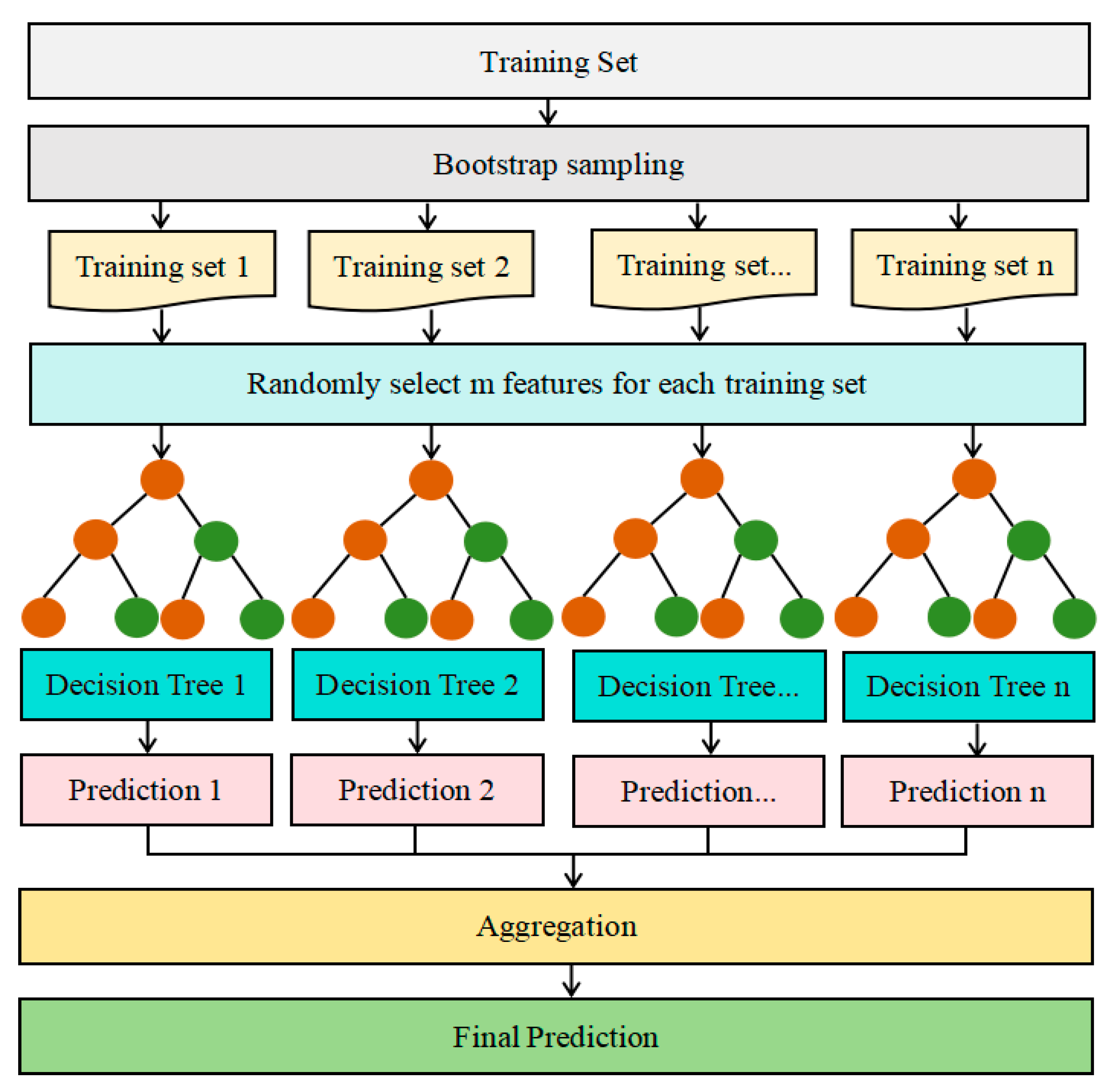
Figure 3.
Prediction performance of 4 models: (a) Comparison of SVR,BPNN and R2; (b) Comparison of PSI.
Figure 3.
Prediction performance of 4 models: (a) Comparison of SVR,BPNN and R2; (b) Comparison of PSI.
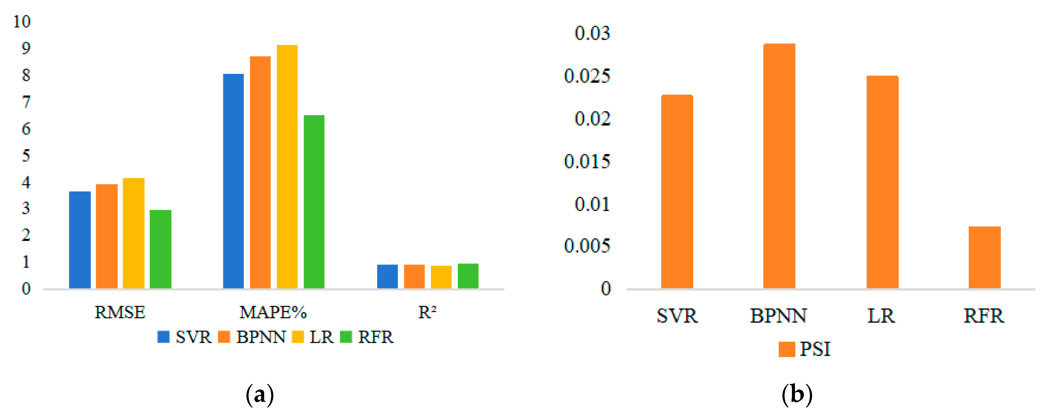
Figure 4.
Prediction result of the test set by RFR.
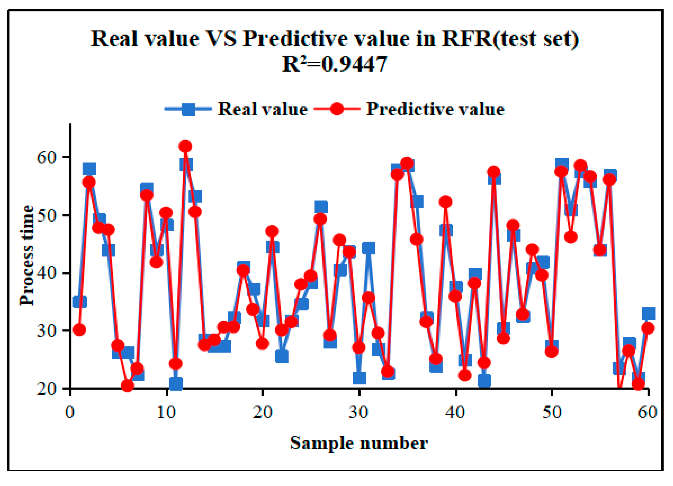
Figure 5.
Prediction result of the test set by SVR.
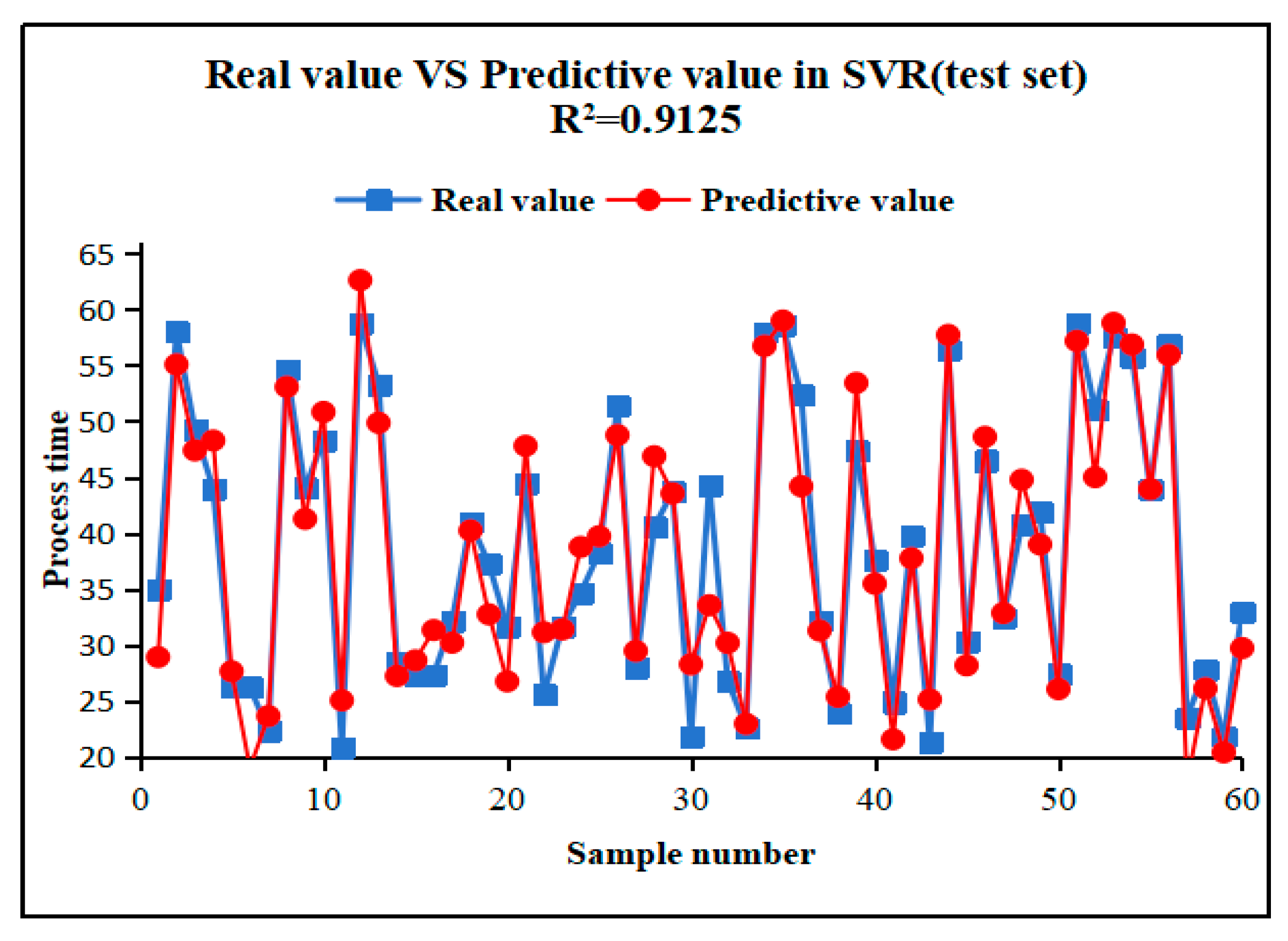
Figure 6.
Prediction result of the test set by BPNN.
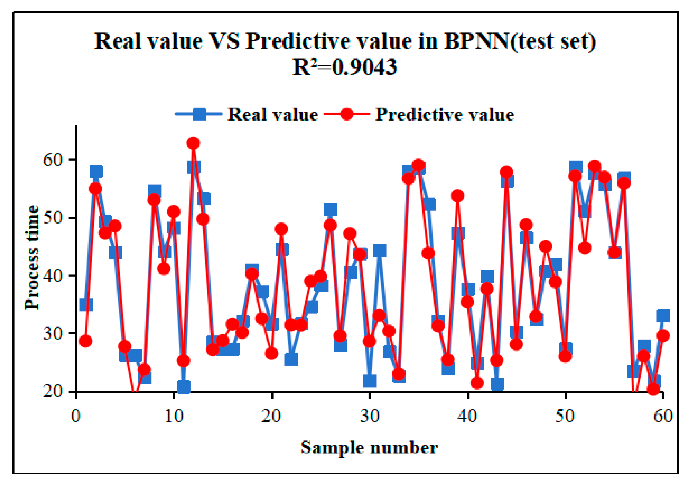
Figure 7.
Prediction result of the test set by LR.
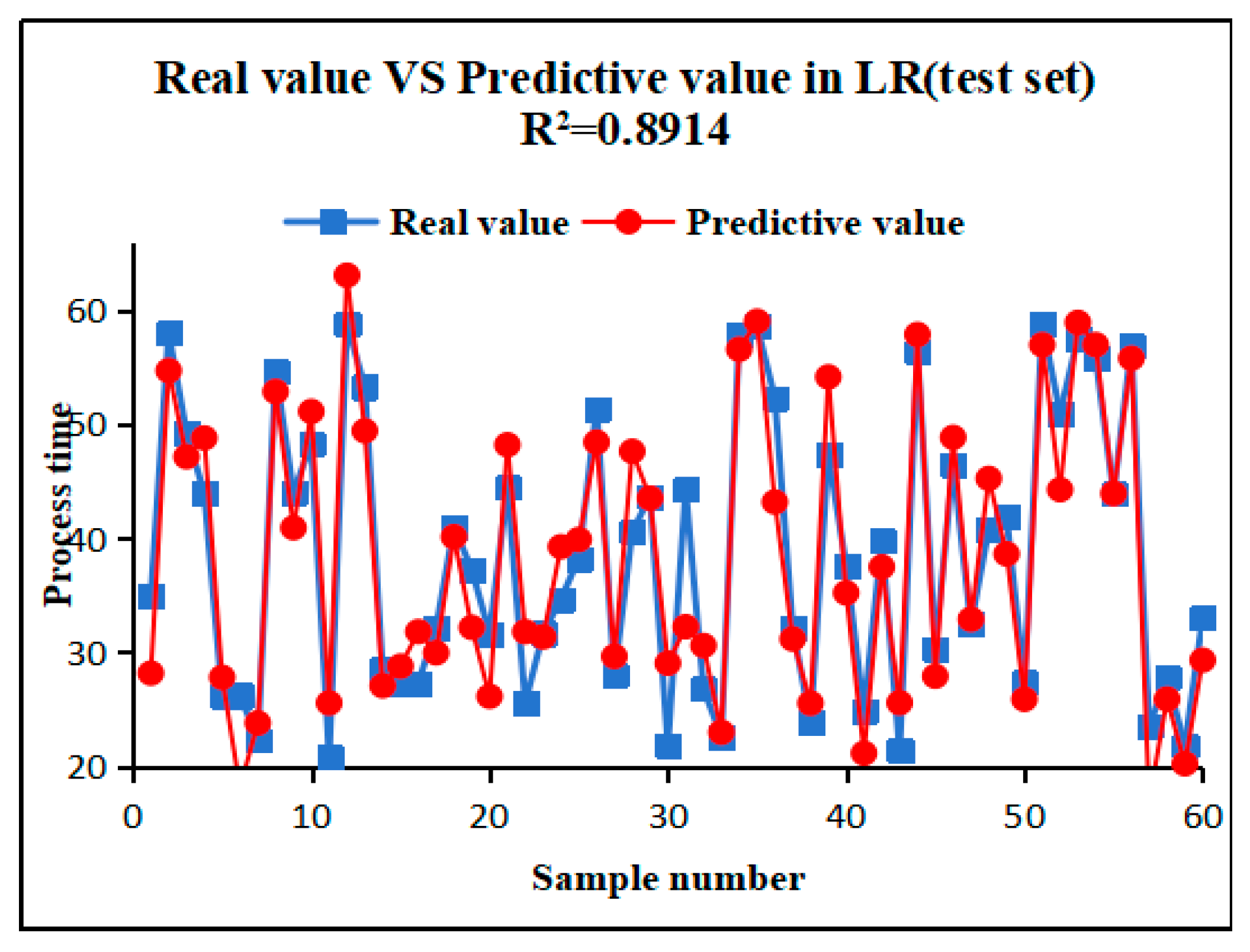
Figure 8.
Relative Error of RFR Predictions.
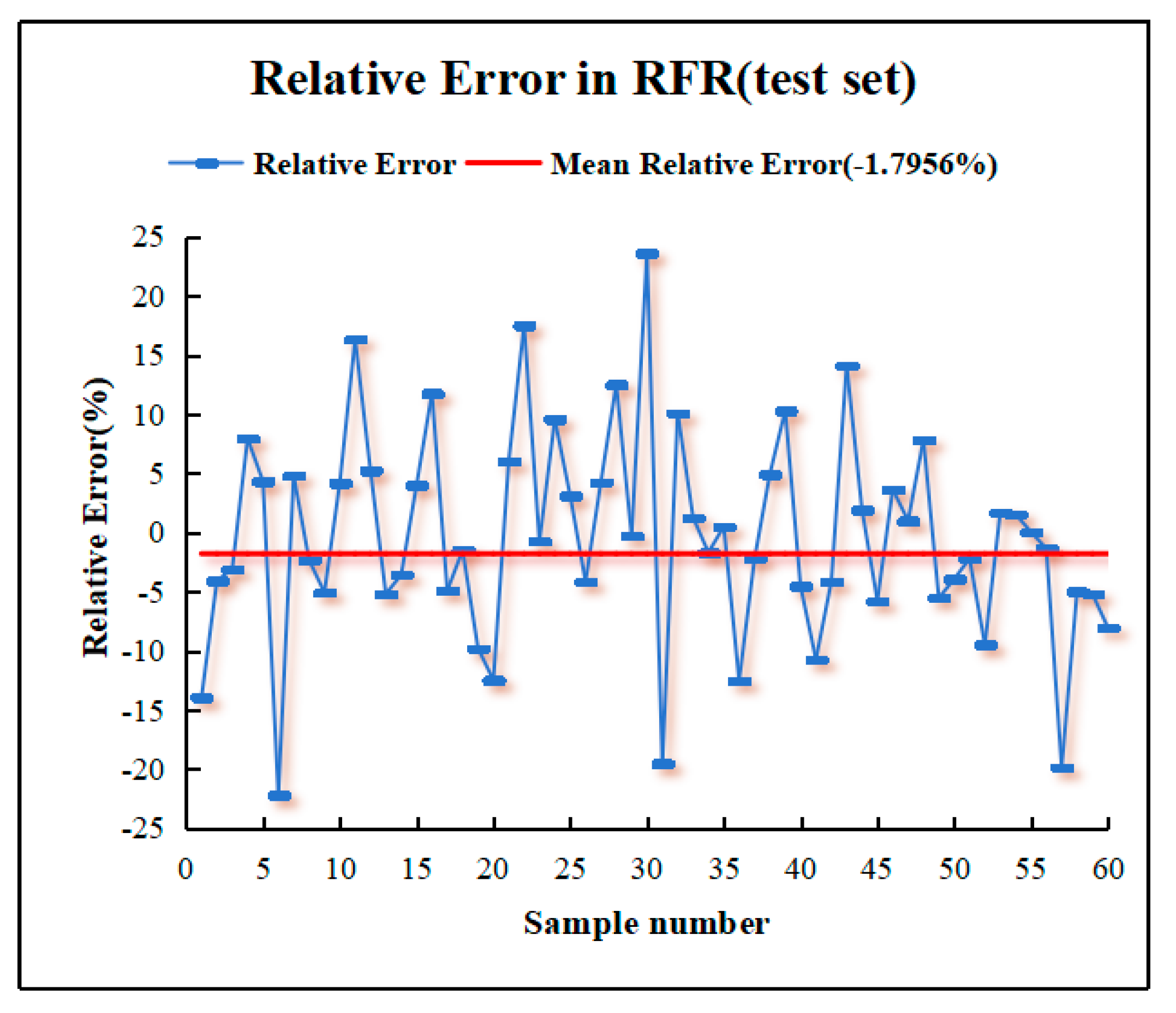

Table 1.
Vairables and their descriptions
| Variables | Variable type | Unit | Description | Labels |
|---|---|---|---|---|
| Man-hour (MH) | Interval | min | Dependent Variable | Y |
| Raw material thickness | Interval | mm | The thickness of raw material steel | X1 |
| Raw material width | Interval | m | The width of raw material steel | X2 |
| Raw material weight | Interval | kg | The weight of raw material steel | X3 |
| Business type | Nominal | — | Including two values:processing, distribution | X4 |
| Allocated length | Interval | m | The length of finished product | X5 |
| Allocated weight | Interval | kg | The weight of finished product | X6 |
| Finished product thickness | Interval | mm | The thickness of finished product | X7 |
| Finished product width | Interval | m | The width of finished product | X8 |
Table 2.
Correlation comparison of different variables
| X1 | X2 | X3 | X4 | X5 | X6 | X7 | X8 | |
|---|---|---|---|---|---|---|---|---|
| Pearson correlation coefficients | 0.0132 | 0.5009 | 0.2104 | 0.3281 | 0.7410 | 0.7326 | 0.0132 | 0.5116 |
Table 3.
Characteristic & Man-hour Data of Samples
| No. | X2(m) | X5(m) | X6(kg) | X8(m) | Man-hour(min) |
|---|---|---|---|---|---|
| 1 | 1.514 | 939.848 | 11170 | 0.755 | 17.48 |
| 2 | 1.072 | 720.422 | 9700 | 1.072 | 23.02 |
| 3 | 1.434 | 528.945 | 10420 | 0.715 | 23.98 |
| 4 | 1.218 | 1133.040 | 9750 | 1.210 | 30.50 |
| 5 | 1.114 | 1109.891 | 8250 | 0.370 | 35.50 |
| ... | ... | ... | ... | ... | ... |
| 26 | 1.386 | 1077.119 | 7172 | 0.460 | 39.00 |
| 27 | 1.278 | 1670.853 | 13410 | 1.270 | 43.00 |
| 28 | 1.514 | 1168.710 | 13890 | 0.755 | 48.00 |
| 29 | 1.278 | 1680.821 | 13490 | 1.270 | 51.00 |
| 30 | 1.534 | 1782.664 | 12880 | 0.765 | 55.00 |
Table 4.
Samples after normalization
| No. | X2 | X5 | X6 | X8 | Man-hour |
|---|---|---|---|---|---|
| 1 | 0.72 | 0.30 | 0.57 | 0.46 | 17.48 |
| 2 | 0.06 | 0.15 | 0.48 | 0.70 | 23.02 |
| 3 | 0.60 | 0.03 | 0.52 | 0.43 | 23.98 |
| 4 | 0.27 | 0.42 | 0.47 | 0.80 | 30.50 |
| 5 | 0.12 | 0.41 | 0.38 | 0.17 | 35.50 |
| ... | ... | ... | ... | ... | ... |
| 26 | 0.53 | 0.39 | 0.76 | 0.23 | 39.00 |
| 27 | 0.36 | 0.78 | 0.72 | 0.85 | 43.00 |
| 28 | 0.72 | 0.45 | 0.75 | 0.46 | 48.00 |
| 29 | 0.36 | 0.79 | 0.72 | 0.85 | 51.00 |
| 30 | 0.75 | 0.85 | 0.68 | 0.46 | 55.00 |
Table 5.
Prediction performance of 4 models
| Model | RMSE | MAPE% | R2 | PSI |
|---|---|---|---|---|
| SVR | 3.65 | 8.03 | 0.91 | 0.0226 |
| BPNN | 3.94 | 8.69 | 0.90 | 0.0286 |
| LR | 4.14 | 9.12 | 0.89 | 0.0249 |
| RFR | 2.96 | 6.51 | 0.94 | 0.0072 |
Table 6.
Interval distribution of PSI values
| Interval No. | Actual | Predict | Actual_rate | Predict_rate | PSI |
|---|---|---|---|---|---|
| 1 | 76 | 69 | 12.83% | 11.67% | 0.001112 |
| 2 | 59 | 54 | 10.00% | 9.17% | 0.000725 |
| 3 | 47 | 58 | 8.00% | 9.83% | 0.003783 |
| 4 | 62 | 65 | 10.50% | 11.00% | 0.000233 |
| 5 | 45 | 42 | 7.67% | 7.17% | 0.000337 |
| 6 | 61 | 64 | 10.33% | 10.83% | 0.000236 |
| 7 | 65 | 63 | 11.00% | 10.67% | 0.000103 |
| 8 | 53 | 51 | 9.00% | 8.67% | 0.000126 |
| 9 | 64 | 68 | 10.83% | 11.50% | 0.000398 |
| 10 | 68 | 66 | 11.50% | 11.17% | 0.000098 |
Table 7.
The comparison of the forecasting results.
| No. | Real man-hour (m) | RFR | SVR | BPNN | LR |
|---|---|---|---|---|---|
| 1 | 20.82 | 24.23 | 25.05 | 25.26 | 21.80 |
| 2 | 26.24 | 27.37 | 27.65 | 27.72 | 18.13 |
| 3 | 31.65 | 27.70 | 26.74 | 31.38 | 35.22 |
| 4 | 34.98 | 30.10 | 28.92 | 38.97 | 39.27 |
| 5 | 38.24 | 39.44 | 39.73 | 39.80 | 36.82 |
| 6 | 43.95 | 47.43 | 48.28 | 43.54 | 32.25 |
| 7 | 49.28 | 47.76 | 47.39 | 47.30 | 51.14 |
| 8 | 51.41 | 49.28 | 48.76 | 48.63 | 44.27 |
| 9 | 54.65 | 53.38 | 53.07 | 56.67 | 52.87 |
| 10 | 58.78 | 57.49 | 57.18 | 59.02 | 56.98 |
Disclaimer/Publisher’s Note: The statements, opinions and data contained in all publications are solely those of the individual author(s) and contributor(s) and not of MDPI and/or the editor(s). MDPI and/or the editor(s) disclaim responsibility for any injury to people or property resulting from any ideas, methods, instructions or products referred to in the content. |
© 2024 by the authors. Licensee MDPI, Basel, Switzerland. This article is an open access article distributed under the terms and conditions of the Creative Commons Attribution (CC BY) license (http://creativecommons.org/licenses/by/4.0/).
Copyright: This open access article is published under a Creative Commons CC BY 4.0 license, which permit the free download, distribution, and reuse, provided that the author and preprint are cited in any reuse.


