
Submitted:
17 October 2023
Posted:
18 October 2023
You are already at the latest version
Abstract
Cycle times at workstations in offsite construction factories fluctuate widely due to various influencing factors. Consequently, relying on average rates, such as length per unit of time, for estimating cycle times proves to be inaccurate, often leading to significant deviations between production schedules and actual operations. To address this issue, this study proposes an estimation system that leverages machine-learning-based prediction, statistical methods, 3D simulation, and computer vision to predict cycle times at the workstation level. Testing of the system on a semi-automated wood-wall framing workstation in a panelized construction factory shows that it reduces the mean absolute error and sum of errors by approximately 36% and 68%, respectively, compared to the fixed rate method. The results also highlight the efficacy of using computer vision data for training machine-learning models for cycle time estimation, the importance of identifying and understanding the factors influencing cycle times, and the impact of random delays on the accuracy of cycle time estimation systems.
Keywords:
offsite construction factories
; cycle time estimation
; machine learning
; computer vision
; 3D simulation
; influencing factors
1. Introduction
1.1. Cycle Time Variability in Offsite Construction Factories
The construction sector has exhibited a trend towards increasing adoption of offsite construction (also known as “prefabricated construction” or “construction manufacturing”), which involves fabricating building components in a controlled factory setting and then transporting them to the construction site for assembly. Shifting towards manufacturing entails adopting principles and methods from manufacturing. In essence, a manufacturing system refers to a “combination of humans, machinery, and equipment that are bound by a common material and information flow” [1]. As such, workers, machinery, and equipment in offsite construction factories are typically positioned in fixed locations at workstations, while production processes (e.g., wall framing, windows/doors installation) are distributed across these workstations. However, in contrast to traditional mass production, offsite construction factories experience significant variability in the cycle times of their processes at these workstations, with cycle time referring to the time spanning from the start to the end of a process cycle. For instance, a recent case study of a panelized construction factory (in which wall panels, floor panels, roof components, and staircases are prefabricated for shipment to the site for installation) reported cycle times for wood wall framing operations ranging from approximately 1 min to as much as 48.5 min [2]. This high variability arises from a variety of influencing factors related to the components, workers, machines, materials, workstation setup, production line, factory operations, and external circumstances [3].
Considering the wide range of cycle times and the multitude of factors influencing them, the current practice in offsite construction of relying on average production rates (such as square footage of a building component per minute) to estimate production time (i.e., the total time required for producing building components) and create production schedules poses certain difficulties. To elaborate, the total production time is contingent on cycle times at various workstations constituting the entirety of production operations. Consequently, overly optimistic cycle time estimates can lead to an underestimation of the time necessary for producing building components, thereby yielding overly optimistic and impractical production schedules. Therefore, an estimation approach is needed whereby process cycle time is estimated for each workstation as a function of the factors influencing it. An overview of related estimation methods explored in previous research is provided in the subsequent subsection.
1.2. Process Time Estimation Methods
Numerous data-driven methods of estimating the durations of construction processes (e.g., machine learning, simulation) have been proposed in the literature, and a variety of different factors influencing the productivity of these processes have been incorporated into the estimation models to improve accuracy. For example, Chao [4] used neural networks (NNs) combined with a simulation model to estimate cycle times of earthmoving operations based on a variety of factors related to the equipment used (e.g., weight of truck), the site conditions (e.g., soil type), and the nature of the operation (e.g., swing angle from truck to cutting location). Zayed and Halpin [5] built simulation models of the piling process to estimate the corresponding productivity, considering equipment-, site-, and operations-related factors. Zayed and Halpin [6] later conducted a similar study to estimate piling process productivity using artificial neural networks (ANNs), while Tam et al. [7] used NNs and regression models to estimate hoisting times of tower cranes considering similar types of factors. In a later study, Tam et al. [8] estimated hook times of mobile cranes as a function of operations and load weight. Many other studies that followed the same line of thinking can be found in the literature (e.g., [9,10]).
Similar estimation methods have been used in industrial construction and offsite construction. For example, Hu et al. [11] followed a similar approach for estimating man-hour requirements for steel fabrication. They trained regression models to estimate man-hours mainly based on design properties, such as the lengths of beams, the quantity of bolts, and the weight of the structure under fabrication. Song and AbouRizk [12] trained an ANN model for estimating steel-fitting activity duration in steel fabrication as a function of design-related factors, such as weight and length, worker skill, as well as work shift. In another study, NNs and multivariable linear regression (LR) models were applied to precast concrete production to estimate productivity in consideration of influencing factors related to product shape, material, and manpower [13,14]. Conducting research on productivity in wood panelised construction, Mohsen et al. [15] trained a number of different machine-learning algorithms to estimate the time required to complete processes on a wall production line as a function of design-related factors (e.g., length, width, number of studs) and factors related to work in progress (e.g., the count of wall panels being processed on the production line). In another recent study in panelised construction, this one targeting the transportation phase, Ahn et al. [16] trained support vector regression models using GPS data in order to predict transportation time for a given project as a function of product-related factors such as the total floor area and total wall area, as well as site-related factors such as location and the maturity of the neighborhood.
However, there is a lack of research that focuses on estimating process cycle time at the workstation level in the production phase for offsite wood construction. A relevant study is the one carried out by Shafai [17] in wood panelized construction. In this study, LR models were developed to estimate the durations of specific tasks (such as spray foam insulation) as a function of the unique design properties of the given panel that are significant to the given task (e.g., number of studs, number of openings, number of cutting zones). Stochastic factors (e.g., triangular distribution) were also incorporated in the regression models to account for uncertainties such as worker performance or machine breakdown. Similar estimation methods have been used in other studies to estimate the processing times at workstations [18,19,20]. Such approaches constitute an improvement upon using a single average value to model the duration of an entire process at a workstation. Nevertheless, further research with a specific focus on cycle time estimation in offsite construction factories is warranted. This is due to the vital role cycle times play in various aspects of production planning and scheduling (as discussed above), as well as in efficiency and optimization in manufacturing settings. This rationale aligns with the availability of research addressing cycle time estimation in other manufacturing settings (e.g., [21,22,23]). Moreover, three related research areas warrant further exploration in the context of cycle time estimation in offsite construction, as explained in the following subsection.
1.3. Research Areas for Further Investigation
1.3.1. Cycle Time-Influencing Factors
Based on the above, the approaches devised for estimating various process time variables mostly rely on machine learning techniques. However, as argued by Benjaoran et al. [13], the reliability of machine-learning models is a function of the exhaustiveness of the influencing factors considered in the models. In this regard, a variety of different factors have been considered in the above mentioned studies, including (1) product-related (or design-related) factors such as number of single studs, double studs, doors, windows, cutting zones, drill holes, nails, screws, etc., for the production of wood wall panels [17], number of fittings and cut-outs for steel fitting [12], number of bolts, length of weld, length of wide flange beams, etc., for structural steel manufacturing [11], and nominal height, weight, and width, concrete volume, finishing area, reinforcement weight, concrete strength, etc., for precast concrete production [13]; (2) worker-related factors such as the number of workers [13], and skill level [12]; (3) material-related factors such as length and weight [11,12]; (4) machine-related factors such as breakdowns [12]; (5) factory operations-related factors such as work shift [12]; and (6) production line-related factors such as activity precedence relationships, queuing, and rework [12].
The benefit of investing effort on identifying these factors is twofold; it not only helps to identify factors that could hold significant information with regards to the estimated process time variable, but also deepens the estimator’s understanding of the process under study. This, in turn, allows the estimator to follow a prescriptive approach for selecting and representing influencing factors used in the machine-learning estimation models [24]. In other words, it enables the estimator to carry out knowledge-driven modelling alongside data-driven modelling, reducing the risk of overfitting to erroneous data patterns or of generating models that cannot be rationally interpreted (compared to an approach that relies solely on empirical data) [24]. Therefore, it is valuable to consider a range of influencing factors and to study their impact on the performance of machine-learning models in estimating cycle times in offsite construction factories.
1.3.2. The Need for Continuous System Tuning
As discussed above, various factors pertinent to the components, workers, machines, materials, workstation setup, production line, factory operations, and external factors influence cycle times. However, if a particular factor remains constant during the timeframe covered in the training dataset, even if it has a significant impact on cycle time, machine-learning models will fail to capture its correlation with cycle time. For instance, suppose an expert worker at a particular workstation is substituted with a less-experienced, less-efficient new employee. In such a scenario, if the dataset used to train machine-learning models for predicting cycle time at that workstation only includes data collected during the tenure of the skilled worker, the models are likely to underestimate the time required to finish a cycle performed by the new employee. In other words, substituting the workers will introduce a new source of variability in cycle time that the models were not trained to capture. In this case, the models will need to be retrained to account for this new variance associated with the employee performing the work. Generally, in order to sustain and enhance the performance of the machine-learning models used to predict cycle times, regular training of the models is necessary. However, consistent training necessitates the ongoing acquisition of training data or, in other words, automated data acquisition. This can be facilitated through the use of computer vision technology, which has shown promise in the context of offsite construction [25].
Computer vision is a branch of artificial intelligence focused on creating autonomous systems capable of imitating specific tasks executed by the human visual system [26]. In computer vision, useful information is extracted from visual components (i.e., digital images, videos, cameras, and closed-circuit television (CCTV)) and is analyzed to facilitate informed, data-driven decisions and recommendations [27]. The field of computer vision has experienced substantial expansion in recent years and is expected to continue growing in the future [28,29,30]. The technology has been successfully implemented in the offsite construction industry for automatically collecting productivity- and progress-related data. For instance, Alsakka et al. [2] deployed the technology to automatically measure the start time, productive time, and cycle time of a wood-wall framing process at a panelised construction factory, achieving a mean absolute error (MAE) of less than 1 min. Zheng et al. [31] used the technology to monitor and track the installation of modules in modular construction projects, as well as to track the duration for which modules are detected in a designated region of interest, achieving a 97.7% accuracy. Wang et al. [32] deployed computer vision for automatically tracking the hoisting and placement of precast concrete wall panels, achieving a precision and recall of 88% and 89%, respectively. Similarly, another study used computer vision to gather timestamp data for precast concrete wall panel installation operations [33]. They succeeded in correctly capturing timestamp data for 10 out of 12 walls using this method [33]. Moreover, computer vision has been employed for measuring the installation rate (cm2/min) of prefabricated panels in panelised construction, achieving an error rate of less than 5% [34]. Finally, Martinez et al. [35] implemented computer vision to track the progress, measure the duration, and calculate the man-hours expended on floor panel fabrication in a panelised construction facility, achieving an overall accuracy of over 92%. Given that computer vision technology has achieved promising performance as exemplified in the aforementioned studies, a further investigation of the performance of machine-learning models trained on computer vision data for estimating cycle times is warranted.
1.3.3. Machine-learning algorithms employed
Another area that merits further exploration relates to the performance of the machine-learning algorithms used in the estimation approaches. While existing methods use LR for building the estimation models, the potential misuse of regression and correlation analysis when the assumptions that underlie them do not hold has been considered in earlier related research (Lu, 2000). Examples of assumptions that may be critical for cycle time estimation in offsite construction given the amount of variability present in operations include the linearity between the predictor variables (i.e., the influencing factors) and the response variable (e.g., cycle time), the independency of observations, and the constancy of the standard deviation and variance of the residuals (i.e., the difference between an observed value and the corresponding predicted value on the regression line) for all values of the predictor variables [36]. Alternatively, NNs are known for their capability to model complex problems, which can be difficult to model using traditional classical mathematical methods [37]. Hence, NNs have been long recognized as a suitable tool for modelling problems in construction research [38], and have found extensive use across various applications, as discussed in the previous section (e.g., [10,12,13,14]). An NN, it should be noted, is defined as “an interconnected assembly of simple processing elements, units or nodes, whose functionality is loosely based on the animal neuron” [39]. Various NNs have been developed to imitate desirable characteristics of the human brain such as its learning ability, generalization capability, and adaptivity [40]. In the aforementioned study by Mohsen et al. [15], however, among the models considered—i.e., random forest (RF), LR, k-nearest neighbor, and NN—the LR model was found to perform slightly better than the NN model when trained on an engineered dataset to predict the production time of wall panels, and the best performing model was the RF model [15].
In light of this and given the variety of influencing factors to be considered in the development of estimation models in this study, further examination of the performance of multiple machine-learning models in estimating cycle times at the workstation level in wood offsite construction, while considering different influencing factors, is warranted. Specifically, based on the results obtained in previous works as explained above, the use of NN, LR, and RF models for cycle time estimation will be explored.
1.4. Study Aim, Objectives and Contribution
The aim of the research presented in this paper, then, was to develop a data- and knowledge-driven system that estimates cycle times considering various influencing factors and using automatically collected data while increasing the estimation accuracy compared to traditional estimation methods. The system was designed to be trained using data collected through a computer vision system and to use machine learning, statistical modelling, and 3D simulation techniques for estimating cycle times at workstations considering a set of cycle-time-influencing factors. The system’s performance was examined through its application to a semi-automated wood-wall framing workstation in a panelised construction factory. In relation to the research needs highlighted above, the secondary objectives underlying this research and the corresponding contributions are as follows:
- (1)
- Examine the effect of considering a variety of influencing factors on the performance of cycle time-estimation models: Doing so helps to demonstrate the importance of expending time and effort on the identification and understanding of influencing factors prior to building prediction models.
- (2)
- Explore the reliability of using data collected automatically through computer vision to train the estimation models: The findings of this task can shed light on the extent to which we can rely on automatically acquired data for building estimation models.
- (3)
- Examine the use of different machine learning algorithms, including the feed-forward ANN, LR, and RF algorithms, for cycle time estimation considering various influencing factors: As discussed in the literature review section above, there is no consensus regarding the behaviour of these machine learning algorithms in the context of process time estimation applications in offsite construction. Therefore, there is merit to gaining a better understanding of how these models perform given various influencing factors in the context of such applications.
The rest of this article is organized as follows: Section 2 provides definitions of the set of process time variables relevant to the developed estimation system, as well as a description of the system and its architecture. Section 3 outlines the procedure followed and methods used to develop the system for the case framing workstation. Section 4 presents the evaluation results of the system’s performance. Section 5 presents an additional analysis of the results with regards to the use of computer vision data, the influencing factors used, the performance of the machine-learning algorithms, and the effect of unpredictable delays on estimation systems. Finally, Section 6 summarizes the findings of the study, discusses implications for the industry, lists the limitations, and suggests avenues for future research.
2. System Description and Architecture
2.1. Process Time Variables
For the purpose of this study, the following definitions of process time variables relevant to the estimation system to be developed were considered. (It should be noted that variations in the definitions of these variables may be found in the literature.)
-
Cycle time (CT): CT refers to the total time spanning from the start of the process undertaken at a workstation for a given component until the end of the process, where a “cycle” refers to the set of tasks assigned to a workstation for a single component (e.g., one wall panel). CT is a function of two variables:
- ∘
- Processing time (PT): PT is the time spent by resources processing a component during a cycle at a workstation. Under ideal conditions, CT is equal to PT.
- ∘
-
Cycle delay (CD): CD is the time during which work is not performed on the component during a cycle at a workstation. In other words, it is the amount of time it takes a cycle to be completed beyond the expected completion time, which is PT. We can further differentiate between two types of delays: predictable cycle delays (PCD) and unpredictable cycle delays (UCD). PCD refers to interruptions to a cycle that can be anticipated and estimated to a certain extent. Examples of PCD include scheduled breaks, meetings, training sessions, predictable unavailability of resources, scheduled maintenance, and waiting for a slow material preparation process. UCD, on the other hand, arises from random events such as machine breakdowns, machine malfunctions, errors in shop drawings, power outages, worker injuries, phone calls, conversing with co-workers, and bathroom breaks.Given these definitions, CT is calculated satisfying Eq. (1).
-
Inter-cycle total delay (ITD): ITD is the total time spanning from the end of a cycle at a workstation to the start of the subsequent cycle. ITD is a function of the following variables:
- ∘
- Downstream-related waiting time (DW): DW is the time spent waiting for the completed component to be transferred to the downstream workstation. Specifically, it is the time spanning from the end of a process undertaken at a workstation to the time at which the component is transferred downstream. Various scenarios could result in DW. One such scenario is when the downstream workstation is busy and there is no inventory between the two workstations or there is inventory that is already at full capacity. Another example scenario that could result in DW is when the resources responsible for transferring the component between workstations are busy with other tasks. Although DW is not factored into the CT for a given cycle, it affects the start time of the subsequent cycle.
- ∘
- Upstream-related waiting time (UW): UW is the time spent waiting (after a completed component is transferred to the downstream workstation) for the upstream workstation to complete work before a new cycle can be started. This occurs when a given workstation is faster than the upstream workstation(s). Since it occurs before a new cycle is started, UW, like DW, is not factored into CT.
- ∘
-
Inter-cycle additional delay (ID): ID is the time by which the start of a new cycle is delayed beyond DW and UW due to any of the aforementioned reasons that cause CD. Note that the total duration of the related delay may be longer than ID, but it may overlap with DW and UW, which is why ID, as defined herein, specifically refers to the additional delay that exceeds the durations of DW and UW. Like CD, ID can arise from both predictable and random events, generally rendering it a random occurrence.Given these definitions, ITD is calculated satisfying Eq. (2).
2.2. System Architecture and Components
The system was designed to be capable of continuously learning from actual process time data and of predicting the process time variables for each component processed at a given workstation as a function of relevant influencing factors. The system’s architecture is displayed in Figure 1, and the major components it comprises are the following (more details are provided in Section 5.3):
- A computer vision system for actual data collection at each workstation: As discussed above, various influencing factors contribute to CT variability in production factories. For this reason, the estimation system should be trained regularly in order to better capture the variability arising from various influencing factors, thus a continuous stream of data from the production factory is required. Therefore, the estimation system uses the computer vision-based time data acquisition system developed in a previous work [2] for automated data acquisition. The system automatically acquires data on the cycle start time, productive time (i.e., the time actually spent by resources working on a component at a workstation—equivalent to PT in the context of this study), and CT for each component processed for a given operation at a workstation.
- A prediction model for PT at each workstation: PT is predictable to a certain degree when the factors that influence its value for a given component at a workstation are known. The degree of predictability, however, may fluctuate at the workstation across different time frames. This is because most of the operations in offsite construction factories are still labour based. Labour-based tasks, even if they are well-defined and standardized, are still subject to high variability because of the inconsistency of human productivity. In fact, PT can even vary for the exact same task depending on the worker’s physical health, mental health, work environment, motivation, and other factors influencing their pace of work. Due to this variability, PT prediction can be highly complex at certain workstations. Nevertheless, machine-learning models can be leveraged to model such complexity. As such, the system developed in the present study uses machine-learning models to predict PT as a function of influencing factors at workstations.
- Estimation models for UCD and ID at each workstation: Given the random nature of the events causing UCD and ID, probability distributions were used to model these variables.
- A 3D simulation model for PCD, DW, and UW: Workstations on a production line affect one another, as the above discussions on DW and UW serve to demonstrate. A simulation model can be used to model the interdependencies among different workstations that determine the durations of UW and DW (which, in turn, affect the start times of cycles). A simulation model can also model the dependencies of workstations on materials/resources, scheduled events, and other forms of PCD. In the present study, a 3D simulation model was used in the estimation system to leverage the benefits associated with its realistic visual representation of the real factory. (Specifically, the 3D visual representation allows the user to determine whether the model is error-free and to validate its representativeness of reality. A 3D model that is developed to be representative of reality also helps users to better understand and analyze the real manufacturing operations.)
The system was developed to include a database serving as a data hub for storing (1) actual process time data measured using the computer vision system, (2) daily production lists of scheduled jobs, (3) panel design properties (e.g., panel length, number of studs) extracted from BIM models, and (4) data concerning other influencing factors.
3. Procedure and Methods for System Deployment
The procedure followed to deploy the system is described in reference to a wall framing workstation at a lightweight wood panelized construction factory. The framing workstation, it should be noted, is the first workstation on a wall production line that comprises several workstations. A portion of this production line is displayed in Figure 2. First, a semi-automated wood-framing machine is used to frame wall panels at the framing workstation, automatically performing nailing, drilling, and cutting operations. An operator loads the machine with framing elements (e.g., single studs, double studs, subassemblies for large doors) when prompted to do so by the machine, which then performs the operations. The wall frame is then transferred to the downstream workstations for further processing. This section describes the steps followed and methods used to deploy the above-described estimation system for the case framing workstation.
3.1. Deploy Computer Vision for Automated Data Acquisition and Manually Collect Data for Testing
The computer vision system developed in a previous work [2] to automatically measure a process’ start time (ST), PT, and CT was deployed for automated data acquisition in the CT estimation system. Data is automatically acquired using computer vision technology through the following approach: In offsite construction factories, work-in-process (WIP) or material flows into and out of workstations in a cyclic manner. This causes specific points along the workstation to cyclically become blocked and unblocked by WIP or material. By strategically placing objects, such as stop signs, at these points, these objects alternate between being blocked and unblocked with each cycle as shown in Figure 3, Figure 4 and Figure 5. Hence, the detection status of these objects can be correlated with the start and end of a cycle, and thus, with ST and CT. This logic was employed to enable the use of object detection algorithms that have been extensively trained to detect objects commonly found in our everyday life using one of the open-source datasets containing a large volume of annotated images of such objects (e.g., [41]). This was aimed to reduce the significant amount of time and effort needed to train object detection algorithms to detect building elements, which may be challenging as they change in shape and size while progressing through the production line. As for productive time, the system assumes that when the worker is detected during a cycle at the workstation, the workstation is actively in use.
The system’s performance was evaluated with reference to its application to the case framing workstation and was found to measure the framing process’ ST, PT, and CT with mean absolute errors that are less than 1 min. In that application, the object detection model YOLOv4 (the fourth version of the “You Only Look Once” object detection algorithm) [42] trained on the COCO dataset [41] to detect commonplace objects was used. Hence, for consistency, the data used for building estimation models in the present article was also collected based on detections made by YOLOv4. Detailed descriptions of the system’s logic, application, and performance can be found in the previous work [2].
The computer vision system was used for automatically collecting data on +200 wall panels framed at the framing workstation. Actual UCD values can be computed by subtracting PT and PCD from CT following Eq. (1). Over the course of the study period, PCDs were limited to scheduled breaks for the case framing workstation. This is because there were no scheduled events that interrupted work, the needed resources were consistently and exclusively dedicated to this workstation (i.e., they are not shared with other workstations), and all of the necessary materials were consistently made ready before they were needed. As such, actual UCD values for the wall panels were measured by subtracting PT and scheduled breaks from CT. To compute ID, ITD can be first computed by subtracting the finish time of a given cycle from the start time of the subsequent cycle. Next, DW and UW can be computed, if they are not null, by considering the finish times of cycles at the upstream and downstream workstations. Finally, the actual ID can be determined by subtracting DW and UW from ITD, according to Eq. (2). Since the framing workstation is the first workstation on the production line, its UW is null as there is no upstream workstation. Meanwhile, the computer vision system has not been implemented yet for the downstream workstation, so no data could be obtained on DW in the present case study. Due to the unavailability of DW data, it was assumed that ID was equal to ITD for the framing workstation for the purpose of building an estimation model for ID. This assumption is not critical, however, since the role of ID in CT estimation is limited to affecting a cycle’s start time which, in turn, may occasionally affect the value of two predictor variables, namely average hourly temperature and work shift, which are used in the prediction of framing CT as described below.
For testing purposes, the variables were also measured manually based on recorded videos of the framing process for additional 40 wall panels.
3.2. Identify Influencing Factors
A multi-stage procedure was followed to devise a list of factors influencing framing CT as described in detail in a previous study [3]. To summarize the procedure, first, a cross-functional diagram of the framing process was mapped in order to gain a deeper understanding of the tasks involved in the process, the resources allocated to it, the manner in which the tasks are carried out, the process inputs, and the process outputs. Eight classes of factors were identified accordingly: “product”, “worker”, “machine”, “material”, “workstation setup”, “production line”, “factory operations”, and “external factors”. Then, factors were identified in relation to each class based on the understanding of the process and a review of relevant literature. The identified factors were then compiled as a list, and a semi-structured interview was conducted to solicit the framing workstation operator’s input on the list. The full list of factors and the interview results can be found in the previous study [3]. Following the operator’s input, some factors, including the availability of shop drawings, learning curve, etc., were eliminated, as they were considered to not affect framing CT at the case workstation. Moreover, since machine learning was only to be used for modelling PT in our system, delay-related factors were also eliminated. Ultimately, the list of influencing factors was narrowed down to 24 features, which are detailed in Table 1, to be considered in the development of the machine learning models.
The framing workstation operator’s input on these features, as described in the aforementioned previous study [3], helped to clarify their consideration as features influencing PT. In what follows we briefly outline some of the reasons for their inclusion. First, the date feature was considered because certain events that occur on specific dates could affect multiple panels, allowing the machine-learning model to identify any patterns or variability associated with particular dates. Panel length was also considered, as longer panels typically require more work. The panel thickness feature was included because thicker elements are heavier and require a larger number of nails. Panel height, meanwhile, was considered, as the framing elements of higher wall panels are heavier. The height difference feature (or delta height) was included since the operator needs to adjust the machine’s opening when panels of different heights are framed sequentially. In relation to this, the framing sequence feature was considered in order to account for any other potential variations in PT resulting from the sequence of the panels. Moreover, the reason why the different types of studs and openings were separated in the list is that they vary in terms of the required numbers of nails, which, in turn, affects the time it takes to nail the framing element. The wall panel design complexity feature was included to reflect the variety of framing tasks that the operator must complete for a wall panel. These tasks could include loading a stud, loading a double stud, loading an L-shaped stud, loading a multi-ply stud, loading a regular door, loading a large door, loading a garage door, loading a regular window, loading a large window, loading a component, performing a cut, drilling a hole, or manually nailing a block (since this task cannot be performed by the framing machine). The wall panel design complexity feature serves to differentiate between a complex wall panel the production of which would necessitate many of these tasks and a simpler wall panel that would necessitate fewer of these tasks. In other words, this feature was included as a way of determining whether it takes the operator more time to interpret the shop drawings and load the requisite elements for more complex wall panels that require more framing tasks compared to less complex wall panels that require fewer types of tasks even if they are of the same size. The work shift feature (morning versus afternoon), meanwhile, was included as a means of determining whether the operator’s work pace changes throughout the course of the day (due to fatigue, for instance). Similarly, the day of the week feature was included as a way of capturing the dynamics of work motivation and fatigue accumulation over the course of the week. The scheduled workload feature was considered as a means of accounting for the possibility that a higher workload puts pressure on the operator to increase their pace of work. The ambient temperature feature, finally, was included by virtue of its potential effect on work pace.
3.3. Prepare Data, Perform Exploratory Data Analysis, and Pre-Process Data
3.3.1. Data Preparation
With the exception of the wall panel design complexity, shift and ambient temperature features, data on the identified features can be extracted from BIM models and from the company’s enterprise resource planning system. In fact, the company’s system supports the extraction of production lists of wall panels scheduled on given dates along with panel design properties into a Microsoft Access database. As such, SQL (i.e., structured query language) queries were developed to combine the data collected on process time variables with the data extracted on the features. However, for the period of operations during which the data was collected, the exported database was missing data on a number of wall panels, which were thus removed from the dataset. The final training dataset contained data on a total of 172 wall panels and the testing dataset contained data on 40 wall panels.
As for the wall panel complexity feature, it was modelled using Eq. (3) as follows.
where is a binary variable that takes a value of 1 if the wall panel includes the corresponding element and a value of 0 if it does not. For the ambient temperature feature, average hourly temperatures were extracted from the Time and Date AS database [43]. Finally, for the shift feature, the value corresponding to each panel was determined based on the start time of its framing cycle.
Following data collection, an exploratory data analysis was conducted to gain understanding of the features, as described in the following subsections. It should be noted that the 24 features included 21 numerical variables and three categorical variables.
3.3.2. Exploratory data analysis
3.3.2.1. Statistical description
Statistical details about these features, as well as about data on PT and CT are provided in Table 1. As presented in the table, the count of non-zero values, mean, standard deviation, minimum value, 25th percentile, 50th percentile, 75th percentile, and maximum value were computed for each feature. Among the various conclusions and observations that could be drawn from these statistics, the ones that stand out with respect to the PT prediction model are the following:
- The range of PT values is wide (i.e., from 1.9 min to 26.8 min), with an average value of 9.3 min for wall lengths ranging from 2 ft to 40 ft and an average length of 30.3 ft.
- The number of panels with large doors, garage doors, preassembled components, double studs, multi-ply studs, and blocks is small relative to the total sample size of 212 wall panels. (Having a small amount of data could compromise accuracy with respect to identifying correlations between the features and the response variable, PT.)
- No wall panels in the dataset were framed on Mondays. As such, any potential effect of this day of the week on PT was not explored.

Table 1.
Dataset description.
| Outcome | |||||||||
| Non-zero count | mean | std | min | 25% | 50% | 75% | max | ||
| PT (minutes) | 212 | 9.3 | 4.0 | 1.9 | 6.7 | 9.3 | 11.5 | 26.8 | |
| CT (minutes) | 212 | 11.6 | 7.5 | 2.3 | 7.7 | 10.2 | 13.4 | 58.4 | |
| Numerical features | |||||||||
| Feature | Non-zero count | mean | std | min | 25% | 50% | 75% | max | |
| 1 | Length (ft) | 212 | 30.3 | 11.8 | 2 | 25.5 | 36.2 | 39.2 | 40 |
| 2 | Height (ft) | 212 | 8.6 | 0.8 | 5 | 8 | 9 | 9 | 10 |
| 3 | Delta height (ft) | 51 | 0.3 | 0.7 | 0 | 0 | 0 | 0 | 4.0 |
| 4 | Thickness (in) | 212 | 5.1 | 1.1 | 3.5 | 3.5 | 5.5 | 5.5 | 7.2 |
| 5 | Regular windows | 37 | 0.3 | 0.7 | 0 | 0 | 0 | 0 | 3 |
| 6 | Large windows | 49 | 0.3 | 0.7 | 0 | 0 | 0 | 0 | 4 |
| 7 | Regular doors | 60 | 0.5 | 0.9 | 0 | 0 | 0 | 1 | 5 |
| 8 | Large doors | 8 | 0.0 | 0.2 | 0 | 0 | 0 | 0 | 1 |
| 9 | Garage doors | 8 | 0.0 | 0.2 | 0 | 0 | 0 | 0 | 1 |
| 10 | Preassembled components | 11 | 0.1 | 0.3 | 0 | 0 | 0 | 0 | 2 |
| 11 | Cutting zones | 150 | 1.9 | 1.9 | 0 | 0 | 2 | 3 | 9 |
| 12 | Drilled holes | 164 | 5.1 | 3.4 | 0 | 2.8 | 6 | 7 | 13 |
| 13 | Studs | 208 | 15.7 | 7.5 | 0 | 10 | 17 | 21 | 34 |
| 14 | Double studs | 14 | 0.1 | 0.3 | 0 | 0 | 0 | 0 | 2 |
| 15 | L-shaped studs | 179 | 2.0 | 1.5 | 0 | 1 | 2 | 3 | 7 |
| 16 | Multi-ply studs | 26 | 0.2 | 0.5 | 0 | 0 | 0 | 0 | 3 |
| 17 | Blocks | 27 | 1.1 | 3.5 | 0 | 0 | 0 | 0 | 32 |
| 18 | Avg hourly temp. (°C) | N/A | 3.9 | 3.4 | −5.5 | 2.5 | 5 | 6 | 12 |
| 19 | Complexity | 212 | 4.4 | 1.6 | 1 | 3.75 | 5 | 5 | 8 |
| 20 | Scheduled workload (sf) | 212 | 14,654 | 2,582 | 11,098 | 12,614 | 14,500 | 16,492 | 21,715 |
| 21 | Panel sequence | 212 | N/A | ||||||
| Categorical features | |||||||||
| Feature | Non-zero count | Categories | Top | Freq. | |||||
| 22 | Day | 212 | [‘Tuesday’, ‘Wednesday’, ‘Thursday’] | Tuesday | 112 | ||||
| 23 | Shift | 212 | [‘Morning’, ‘Afternoon’] | Afternoon | 125 | ||||
| 24 | Date | 212 | [‘2022-03-15’, ‘2022-03-16’, ‘2022-03-22’, ‘2022-03-23’,’2022-03-24’, ‘2022-03-29’, ‘2022-03-30’, ‘2022-04-05’] | 2022-03-16 | 41 | ||||
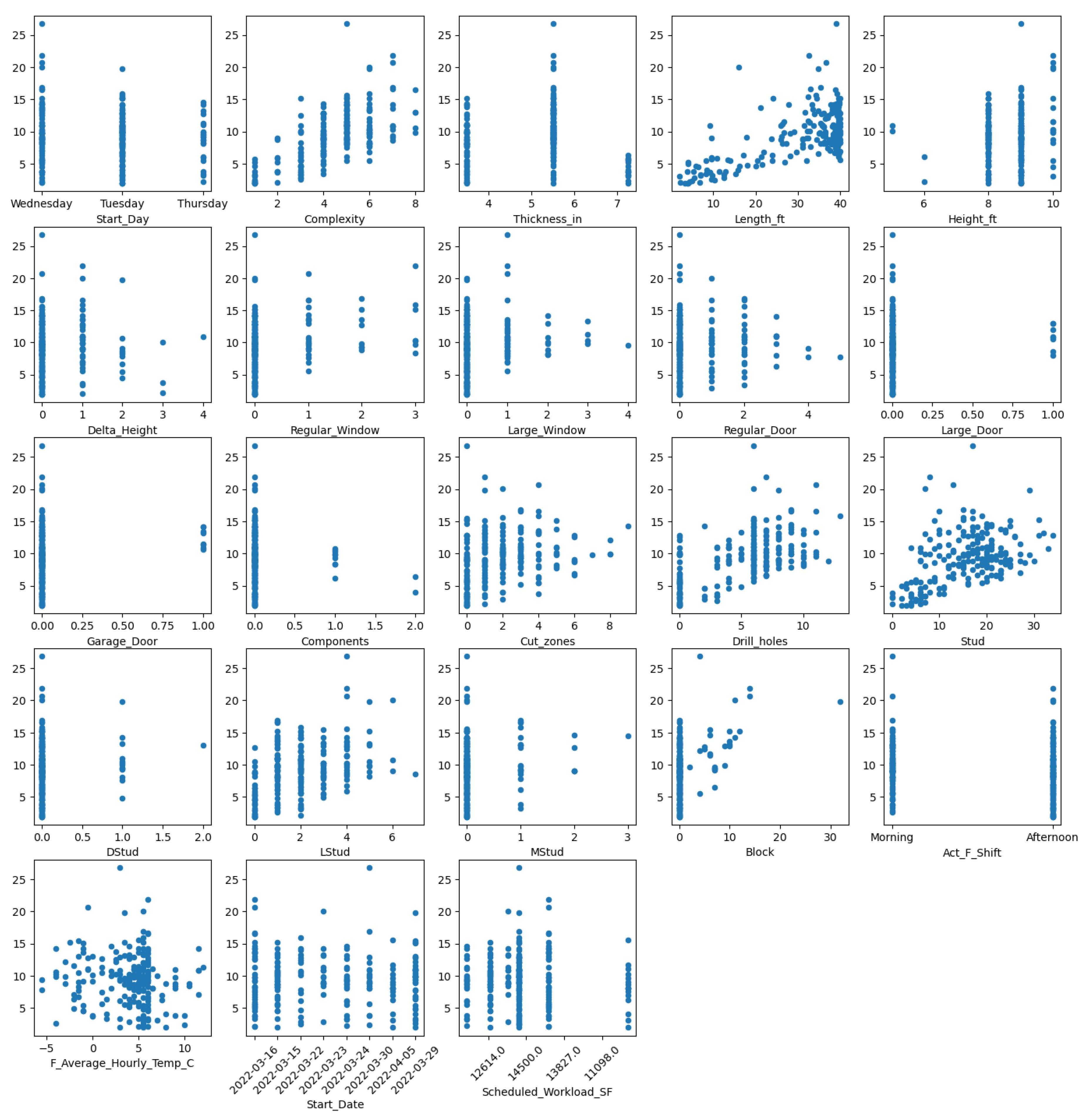
3.3.2.2. Correlation with PT
Moreover, in order to identify key features affecting PT, scatter plots and Spearman’s rank correlation coefficients were analyzed (Figure 4 and Table 2). Scatter plots were drawn in order to visualize the relationship between each feature and PT, while Spearman’s rank correlation coefficients were computed in order to determine the strength and direction of the correlations. By identifying these correlations, we were able to gain insights into which features were strongly associated with PT and, in turn, use this information to guide the machine-learning process. Of the features analyzed, complexity, length, all types of studs, number of drilled holes, number of cutting zones, blocks, garage doors, and windows all showed clear correlations with PT, while weaker correlations were observed with the other features. (However, it is important to note that an NN model, for example, may still be able to identify more complex relationships between these features and PT.) Based on these results, no features were removed from the analysis, as all may provide valuable information to the machine-learning models. Instead, the correlations identified served to guide the decisions on feature selection in order to optimize the accuracy and efficiency of the machine-learning models.
Table 2.
Spearman’s coefficient.
| Feature | Spearman’s coefficient | Feature | Spearman’s coefficient |
|---|---|---|---|
| Complexity | 0.63 | Multi-ply studs | 0.17 |
| Drilled holes | 0.54 | Large doors | 0.10 |
| Length (ft) | 0.49 | Regular doors | 0.10 |
| Studs | 0.42 | Double studs | 0.10 |
| L-shaped studs | 0.39 | Height (ft) | 0.08 |
| Blocks | 0.35 | Delta height (ft) | 0.05 |
| Cutting zones | 0.31 | Thickness (in) | 0.04 |
| Regular windows | 0.28 | Scheduled workload (SF) | −0.02 |
| Large window | 0.20 | Preassembled components | −0.06 |
| Garage doors | 0.20 | Avg hourly temp. (°C) | −0.11 |
Figure 4.
Scatter plots.
3.3.2.3. Multicollinearity
The use of LR for predicting PT being one of the prospective solutions to be tested, the variance inflation factor (VIF) was computed for the numerical features in order to measure the degree of multicollinearity between different features. VIF was selected as a diagnostic tool for multicollinearity because it provides interpretable information about the regression coefficients [44]. For example, a VIF of 10 means that the variance of the coefficient of the independent variable is 10 times greater than it would have been if this variable had been linearly independent of the other variables [44]. The results are provided in Table 3. As shown in the table, height, length, complexity, scheduled workload, thickness, stud, and number of drilled holes were the features found to have the highest VIF values. This finding can be attributed to the following: (1) longer panels typically have a greater number of studs; (2) longer panels typically require a greater number of holes to be drilled for installing hooks for lifting; (3) the complexity feature is a function of the framing elements, as per Eq. (3); (4) the scheduled workload is constant on each date; and (5) longer panels usually consist of multiple interior walls that are framed together, whereas most interior walls are shorter and less thick. No features were removed at this juncture based on VIF results. Rather, the values helped to aid understanding of the results of the LR model.
Table 3.
VIF for features.
| Feature | VIF | Feature | VIF |
|---|---|---|---|
| Height_ft | 80.5 | Large_Window | 2.9 |
| Length_ft | 60.7 | Regular_Door | 2.7 |
| Complexity | 48.6 | Regular_Window | 2.0 |
| Scheduled_Workload_SF | 42.2 | Start_Day_Thursday | 1.6 |
| Thickness_in | 36.9 | Block | 1.6 |
| Stud | 31.2 | Large_Door | 1.4 |
| Drill_holes | 11.7 | Delta_Height | 1.4 |
| Act_F_Shift_Afternoon | 6.0 | DStud | 1.4 |
| F_Average_Hourly_Temp_C | 5.8 | MStud | 1.4 |
| LStud | 4.0 | Preassembled components | 1.3 |
| Cut_zones | 4.0 | Garage_Door | 1.3 |
| Start_Day_Tuesday | 3.3 |
3.3.3. Data Pre-Processing
To ensure that features with higher scales such as the scheduled workload and length features do not dominate the learning process of the estimation models, numerical features were scaled to have a mean value of 0 and a standard deviation of 1. As for transforming categorical features, the one-hot encoding technique was used where each category of a feature was transformed into a binary variable (i.e., separate column) in the dataset. For example, the afternoon shift was added as an additional binary column in which a value of 1 indicates an afternoon shift and a value of 0 indicates a morning shift since there are only two categories for the shift feature. Since a value of 0 in the afternoon shift column indicates a morning shift, including a column for the morning shift category would introduce redundancy in the dataset. Hence, for each categorical feature, one binary variable was dropped to avoid multicollinearity between the introduced binary variables.
3.4. Select Performance Evaluation Metrics
The following metrics were used to evaluate performance and calculate errors at different stages in the study.
- The prediction error, , was calculated satisfying Eq. (4). This metric was selected to examine whether the predictions tended to overestimate (positive error value) or underestimate (negative error value) true values, as well as to determine the degree of variance of the measures from their true values for each panel.where is the prediction error corresponding to panel , is the predicted value for panel , and is the actual value corresponding to panel .
- The sum of errors, SE, was calculated satisfying Eq. (5). This metric was used to evaluate whether the predictions made for a batch of panels are cumulatively overestimated or underestimated.where is the total number of panels used for evaluation.
- The MAE was calculated satisfying Eq. (6). This metric was used to determine the average degree of variance of the predictions from their true values, regardless of whether they had been overapproximated or underapproximated.
- The mean percentage error (MPE was calculated satisfying Eq. (7). This metric was used to evaluate the prediction errors as a percentage of the true values.
- The root mean squared error (RMSE) was calculated satisfying Eq. (8). This metric was used in addition to MAE as it is useful for detecting outlier values since it assigns a higher penalty to larger errors compared to MAE.
3.5. Build PT Prediction Models
As noted above, the data used for training the machine-learning models was automatically collected using the computer vision system. A 10-fold cross validation was employed to tune the parameters of the models and select features based on RMSE and MAE values. The training results are described in this section, while the testing results are described later in Section 4.1.
3.5.1. Artificial Neural Network Model
A multi-layer feed-forward ANN model was trained using the open-source machine-learning platform, H2O [45], accessed through Python, in order to predict PT. The Cartesian grid search method, in which a set of values is specified for each hyperparameter under which to search [46], together with a trial-and-error approach, was employed to select values for the model’s hyperparameters, two hidden layers with 200 neurons each were ultimately incorporated into the model, and ten epochs were used for training. The activation function that resulted in the best performance based on cross-validation results was the “tanh” function implemented in conjunction with dropout regularization, which helps to reduce overfitting by randomly dropping out neurons during training. Moreover, the “Laplace” distribution was found to achieve the best results and thus was used in the model.
All 24 features were initially included in the model, which yielded an RMSE of 2.67 min and an MAE of 1.91 min based on cross-validation results. The importance of features was calculated following the Gedeon method, which measures the contribution of an input neuron to an output neuron in an NN [47]. The scaled importance of features was found to range from 0.61 to 1.0, with complexity, length, and block having the highest importance (1.0, 0.901, and 0.896, respectively), and the other features ranging in importance from 0.615 to 0.752. All of the values were relatively close to one another, and the model was found to perform more poorly when testing the removal of the features with the lowest importance. Hence, the correlation results presented in Section 3.3 were used in a trial-and-error approach to evaluate whether removing certain features could improve the model’s performance. The scheduled workload feature was the first feature to experiment with due to the lack of a clear relationship between this feature and PT, as evidenced by the null Spearman’s coefficient and the absence of a clear pattern in the scatter plot. Indeed, the removal of this feature reduced the RMSE and MAE to 2.60 min and 1.80 min, respectively, leading to the decision to remove it from the model. The same experiment was conducted for the thickness, delta height, preassembled components, and height features, given their low Spearman’s coefficients of 0.04, 0.05, −0.06, and 0.08, respectively. However, the removal of these features led to increases in RMSE and MAE of 2.69 min and 1.88 min, 2.72 min and 1.90 min, 2.76 min and 1.93 min, and 2.79 min and 1.96 min, respectively. The next feature to experiment with was the shift feature, since no clear relationship could be identified between this feature and PT based on the scatter plot. Nevertheless, removing the shift feature increased RMSE and MAE to 2.77 min and 1.88 min, respectively. Following that, given the small number of panels with large doors (eight panels only), the regular doors and large doors features were combined into one feature, referred to simply as “doors”. This resulted in increases in RMSE and MAE of 2.71 min and 1.92 min, respectively. It is worth noting that, when the framing elements (i.e., studs, D-studs, M-studs, large windows, etc.) were combined into a single feature following the approach outlined in the study by Mohsen et al. (2022) and used along with the remaining features in the model, the resulting error was higher compared to when including all 24 features, with the RMSE measured at 3.04 min and the MAE at 2.26 min.
In general, the removal of any of the 23 features other than the scheduled workload feature resulted in a decline in the model’s performance, indicating the importance of these features. Therefore, all features other than the scheduled workload feature were retained in the NN model, resulting in an RMSE of 2.60 min and an MAE of 1.80 min.
3.5.2. Linear Regression Model
An LR model was developed using the RapidMiner software [48]. All features with the exception of the date feature were initially included in the model, which yielded an RMSE of 2.83 min and an MAE of 2.18 min based on the cross-validation results. However, the p-values corresponding to the regression coefficients were found to be greater than 0.10 for all the features other than the block, length, complexity, number of cutting zones, and day of the week features, indicating that the coefficients may not be statistically significant and that the observed relationship between the feature and PT may be due to chance. (It is interesting to note that length, complexity, and block were the most important features based on the Gedeon method and had the most statistically significant regression coefficients in the LR model.) Next, the effect on the model’s performance of removing less significant features was examined in an iterative manner based on cross-validation results. With each iteration, the feature with the highest p-value was removed and, if the model’s performance improved, the feature was then excluded from the model in subsequent iterations. The features removed, in order of their removal, were large doors, large windows, shift, sequence, regular window, stud, regular door, scheduled workload, height, number of drilled holes, D-stud, ambient temperature, and L-stud. Ultimately, the LR model was reduced to include a limited number of features beyond which removing any feature resulted in increased errors, as expressed in Eq. (9). This streamlined LR model yielded an RMSE of 2.61 min and an MAE of 2.00 min based on the cross-validation results.
While the M-stud, garage door, and delta height features all had p-values greater than 0.10, in each case the feature’s removal was found to negatively affect the performance of the LR model, indicating its importance in predicting PT. The remaining features all had p-values less than 0.04, indicating their significance based on a 5% significance level. The effect on the LR model’s performance of combining the framing features was also examined since following this approach improved the performance of the LR model in [15]. However, no improvement was observed in the model’s performance using this approach, where the lowest RMSE and MAE were measured at 2.71 min and 2.10 min, respectively. The best-performing LR model remained the one presented in Eq. (9), but it performed more poorly than the NN model based on cross-validation results.
3.5.3. Random Forest Model
An RF model was trained using the open-source machine-learning platform, H2O, accessed through Python, to predict PT. The Cartesian grid search method together with a trial-and-error approach, was used to select values for the model’s hyperparameters. Ultimately, 50 decision trees, each with a maximum depth of 20, a minimum number of rows of 5, and a row sampling rate of 0.8, were selected based on the cross-validation results. The RF model containing all 24 features yielded an RMSE of 2.88 min and an MAE of 2.13 min.
The H2O platform, it should be noted, calculates the importance of each feature as the total improvement in the squared error realized following splits of the trees on the feature [49]. Unlike in the case of the NN model, here the results showed a wide range of importance values for different features. The length feature had the highest importance score, scaled to 1.0, followed by the complexity feature with a scaled importance of 0.59. The importance scores of the number of drilled holes, stud, block, and L-stud features ranged from 0.15 to 0.39, while the number of cutting zones, height, and ambient temperature features had scores ranging from 0.05 to 0.39. The remaining features had importance scores lower than 0.04, with some (i.e., the large window, shift, regular door, D-stud, garage door, preassembled components, and large door features) even below 0.01. However, these scores may not necessarily reflect the true significance of the features in relation to PT, as it was observed that the features with the lowest number of observations—there were only eight large doors, eight garage doors, and 11 preassembled components in the entire dataset—tended to have the lowest importance scores. For example, garage doors had an importance score near 0 when, in reality, garage doors have a significant effect on PT since they necessitate manual work (which cannot be completed using the framing machine), as also evidenced by the statistically significant regression coefficient shown in Eq. (9). The RF model was reduced to exclude all the features with low importance. As such, the final model included the length, complexity, number of drilled holes, stud, block, L-stud, and number of cutting zones features and yielded an RMSE of 2.83 min and an MAE of 2.11 min. The RF model performed more poorly than both the NN and LR models based on cross-validation results.
3.6. Develop UCD and ID Estimation Models
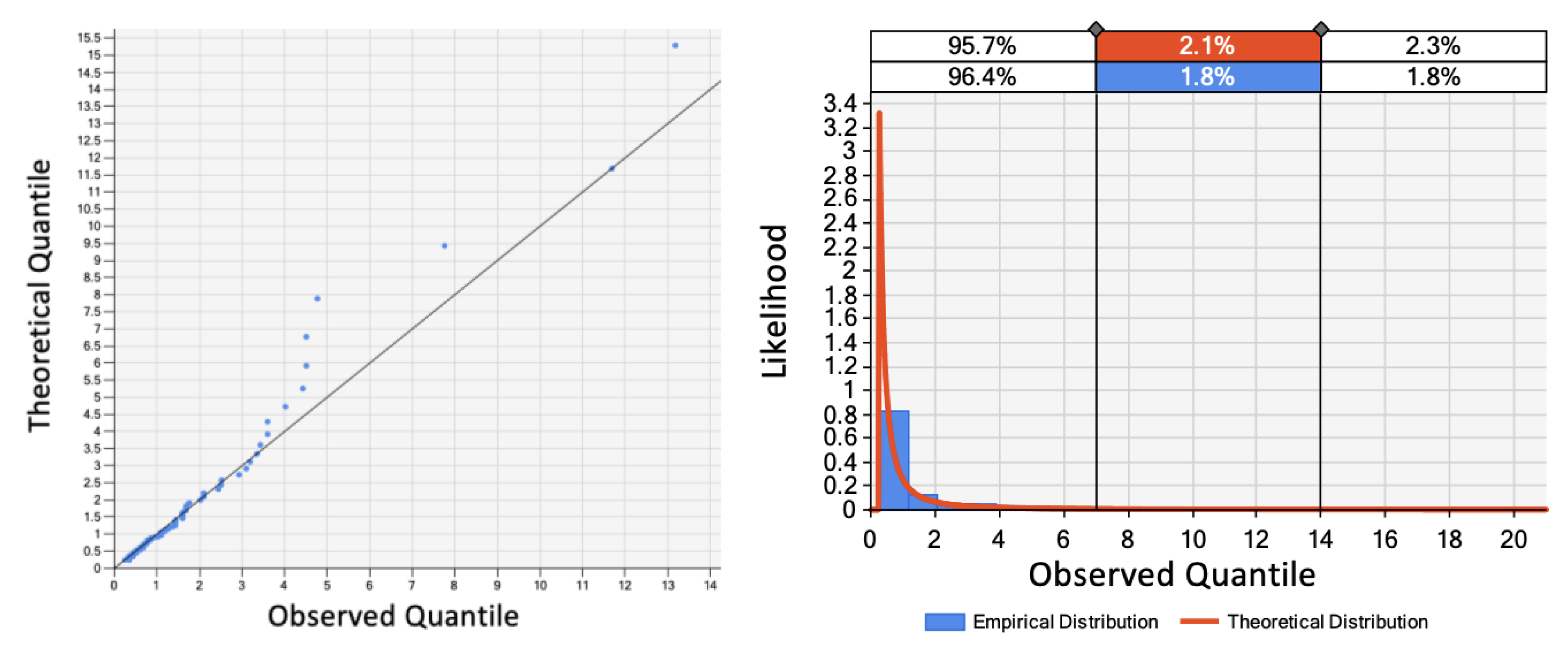
As previously explained, UCD could be computed by subtracting PT and scheduled breaks from CT for the case framing workstation. As such, UCD was evaluated for the 172 panels included in the training dataset and used to fit statistical distributions in Simphony.NET software [50]. The least squares method [51] was used to fit a set of distributions, and the Kolmogorov-Smirnov (K-S) test was performed in Simphony.NET to evaluate how well the distributions fit the data. The K-S test is based on the maximum difference between the empirical and theoretical cumulative distributions [52]. Based on the results, the Pareto distribution with a shape parameter of 0.94 was found to provide a good fit for the data, as also indicated by the Q–Q plot, shown in Figure 4, since most of the points on the Q-Q plot were found to fall close to the diagonal line. However, some points were found to fall well above that line, indicating that the corresponding values in the dataset are smaller than what would be expected under the assumed distribution. This suggests that the actual data has a lighter tail than the Pareto distribution, as also confirmed by the Pareto’s probability density function plotted against the empirical distribution in Figure 4. As such, to avoid sampling extreme UCD values from the Pareto distribution, which do not accurately represent reality, a trial-and-error approach was followed to cap random sampling in a manner that would minimize MAE and SE. Ultimately, sampling was capped at 4 min, beyond which the Pareto distribution consistently overestimated the observed values as indicated by the Q-Q plot. Capping the sampling process was accomplished by rejecting any sampled values greater than 4. It should be noted that using a cap of 4 min means that actual UCD values exceeding 4 min will be underestimated by the system. However, the occurrence of such events is relatively minimal based on the training data. Moreover, these occurrences should be addressed through proper control of operations rather than adjusting the system, as discussed later in this article.
The Simphony.NET software, the least squares method, and the Kolmogorov-Smirnov (K-S) test were similarly used to build a statistical model for ID. The Chi-squared distribution with two degrees of freedom was found to have the best goodness-of-fit for modelling ID.
Figure 5.
Pareto distribution fitting.
3.7. Build the Simulation Model
A 3D simulation model was developed for the entire wall production operation using Simio software [53], as shown in Figure 6. The simulation model was connected to an MS Access database from which it could retrieve the list of wall panels scheduled for the day as well as data on the corresponding features. Based on a predefined production sequence, the model was developed to mimic actual operations and simulate the production of wood wall panels as they flow from one workstation to another. At the framing workstation, PT, UCD, and ID were modelled using the NN model (selected based on the results presented in Section 4 below) and the statistical models previously developed, respectively, while the simulation model was mainly responsible for (1) determining when a framed wall panel could be transferred to the downstream workstation and, accordingly, when a new framing cycle could be started, (2) halting production during scheduled breaks, and (3) collecting data on cycle start time (ST), finish time (FT), CT, PT, CD, DW, and UW, as shown in Figure 7. The remaining workstations were modelled by incorporating regression and statistical models developed by Shafai (2012) in a prior study conducted on the same case production line. (The regression models predict the durations of various tasks performed at each workstation as a function of wall panel design attributes, and the statistical models estimate delays. However, these models provide only rough estimates of the current cycle times of downstream workstations, and this is a limitation of the present study, as discussed in the Limitations subsection below.)
The simulation model was verified and validated in several ways. First, the model was developed in stages with weekly meetings conducted with the case company’s research and development personnel who, at each stage, validated that the model reasonably represented actual operations. Second, the 3D animation functionality of the model significantly facilitated verifying that the model was behaving as intended and validating that it was representative of actual operations as it enabled a direct comparison between virtual operations within the model and actual images captured of real operations. Third, the data collected during simulation, as depicted in Figure 5, Figure 6 and Figure 7, provided further support for verifying the model’s sound behavior. Finally, CT estimates generated by the model for forty wall panels were compared to actual measurements. The obtained results, which are detailed in the following section, further validated the soundness of the model.
Figure 7.
Sample simulation data.

4. System Testing Results and Discussion
The performance of the PT and CT predictions was evaluated using the testing dataset manually collected for 40 wall panels, as described in greater detail below. Moreover, the case company uses a linear fixed rate (meters per minute) to estimate the full production capacity of the wall production line under ideal conditions, and was developing production schedules at the time of the present study based on the assumption that the production line was operating at 85% of its full capacity. The performance of the case company’s current estimation practice was also evaluated, as described later in this section.
4.1. Evaluation of PT Predictions
The PT prediction performance of each of the three models and of the current estimation practice at the case company are summarized in Table 4. As these results show, the LR model was found to have the best performance, with MAE, MPE, and SE values of 1.52 min, 19%, and 5.62 min, respectively. However, based on MAE and MPE only, the NN and LR models achieved similar levels of performance. Meanwhile, the RF model showed the poorest performance based on MAE and MPE (i.e., 1.81 min and 21%, respectively), although it achieved a lower SE than did the NN model (10.01 min in the case of the former versus 17.68 min in the case of the latter). The SE was positive for each of the three models since the overestimations tended to be more frequent (and in some cases more significant) than the underestimations. Although the NN and LR models were found to be comparable in performance based on MAE and MPE, the NN model had a larger SE since the overestimations it made were larger than the overestimations made by the LR model. Similarly, the size of underestimations made by the LR model was larger than that of the underestimations made by the NN model. This difference is clear in Figure 8. It is also worth noting that errors corresponding to four of the panels framed sequentially skewed the evaluation results, as the prediction error of these panels ranged between 2.66 min and 4.94 min for the NN model, between 2.51 min and 3.86 min for the LR model, and between 2.62 min and 3.86 min for the RF model. Excluding these panels from the evaluation reduced the MAE, MPE, and SE to 1.31 min, 15%, and 1.99 min, respectively, for the NN model, to 1.33 min, 16%, and −7.30 min, respectively, for the LR model, and to 1.67 min, 19%, and −2.37 min, respectively, for the RF model. In other words, with this outlier sequence of four panels removed, the NN model showed the best performance based on the testing results. In examining the recorded framing processes for these panels, no satisfactory explanation for the high error values could be identified aside from the fact that the operator was consistently working at a high speed when framing them. Another potential explanation of the high error values could be the presence of similar panels that took longer to frame or panels for which the computer vision system overestimated the actual PT values in the training dataset. Whatever the cause of the high error values, in future when the system is deployed for continuous data collection, the size of the training dataset will be continuously increasing, and this should improve the performance of the models as they continuously learn from new data.
To summarize, based on the cross-validation results, among the three models considered it was the NN model that was found to perform best. Although it was the LR model that performed better based on the preliminary analysis of the testing results, the NN model would have outperformed the LR model if it had not significantly overestimated the PT values for the four panels with high errors. In general, the NN model tended to overestimate PT more than did the LR model. However, since capping the UCD values may lead to underestimating long delays, occasional overestimations of PT would reduce SE for the daily scheduled batch of panels. Moreover, an estimation system that tends toward overestimation of PT is preferable to one that tends toward underestimation of PT (since the former gives more conservative estimates). As such, the NN model was selected for use in the estimation system.
Finally, the case company’s current estimation practice was found to have an MAE of 2.87 min and an MPE of 29%, while the SE was negative (approximately −99 min). The SE was significantly negative due to the frequency and size of underestimations made based on the fixed rate assumption. In fact, the current estimation practice underestimated PT for 32 of the 40 panels, indicating that the fixed rate assumption is overly optimistic. In other words, all three machine-learning models outperformed the current estimation practice in estimating PT, with the NN model and the LR achieving reductions in MAE of 45% and 47%, respectively, compared to the current practice.
4.2. Evaluation of CT Predictions
The evaluation of the CT predictions and of the current estimation practice are summarized in Table 5. As can be seen, the estimation system achieved an MAE of 3.03 min and an MPE of 23%, while the SE was negative (i.e., −50 min), although the number of panels with overestimated predictions was equal to the number of panels with underestimated predictions (i.e., 20 panels). The negative SE was due to the larger size of underestimations compared to overestimations. This discrepancy is partly attributable to the UCD predictions having been capped at 4 min, resulting in two error values of about 17 min. The actual UCD values for these two panels were around 14 min and 16 min, as the operator had left the workstation during the framing process in both cases. Omitting these two panels alone reduced the MAE, MPE, and SE to 2.30 min, 21%, and −16.28 min, respectively. Moreover, although the SE of −16.28 min implies that the estimation system slightly underestimated the total time needed to frame a batch of panels, this underestimation is insignificant compared to the total actual time spent on framing 38 panels (i.e., about 420 min).
Nevertheless, notwithstanding the higher CT prediction errors, the developed estimation system performed significantly better than the current estimation practice, which yielded an MAE of 4.72 min, an SE of −156 min, and an MPE of 34%. In other words, the estimation system realized reductions in MAE and SE of about 36% and 68%, respectively, compared to the current estimation practice. The current estimation practice was found to significantly overestimate the actual capacity (or underestimate cycle times) of the framing workstation. Meanwhile, the framing workstation is the first workstation on the production line, so the actual production capacity of the wall production line should be less than or close to that of the framing workstation. This means that the overall production capacity of the whole production line is overly optimistic in current practice. An overly optimistic estimation of production capacity leads to a scenario in which more panels per day are scheduled for production than what can be produced, in turn resulting in production targets being missed and in a physical and mental toll on the well-being of workers. In this regard, it is notable that the developed estimation system was found to significantly outperform the current practice.
5. Further Analysis of the Findings
5.1. Use of Computer Vision Data
The prediction error of the three models may be partly attributable to measurement errors on the part of the computer vision system. Specifically, the frequency, and, for some panels, the size, of overapproximations made by the models were greater than those of the underapproximations. Meanwhile, the size of the PT overapproximations made by the computer vision system, as reflected in the results of a prior study [2], was generally greater than that of the underapproximations. As such, the overapproximations on the part of the prediction models may be partially attributable to the fact that PT was more significantly overapproximated than underestimated by the computer vision system for a number of panels in the training dataset. Nevertheless, the fact that the performance of the three machine-learning models was superior to that of the fixed rate used in current practice points to the suitability of using computer vision data for training the models in applications of this nature. Indeed, computer vision is a promising solution, as it provides a practical and time-efficient supply of data that can be used to continuously tune the models in order to account for future sources of variability.
5.2. Influencing Factors
As noted above, the features considered in the machine-learning models were initially identified based on a detailed qualitative analysis of the framing workstation as outlined in a previous study [3]. Interestingly, all of the features with the exception of the scheduled workload feature were found to hold relevant information regarding PT in at least one of the machine-learning models. Notably, the NN model found all of the features, with the exception of the scheduled workload feature, to be significant predictors of PT. However, this does not necessarily imply that scheduled workload does not affect PT. In fact, the data collected for this case study only covered days of operations that resulted in a limited number of observations for this feature. Since any potential effect of workload on PT would be indirect, several months’ worth of data may be necessary to ascertain whether or not it has an impact. Moreover, although the majority of the features were found not to have a statistically significant regression coefficient in the initially developed LR model, a number of them were found to have a potentially explainable effect on PT. The LR model trained using all features is expressed in Eq. (10).
As explained in Section 3.2, the increase in length, height, and thickness should logically increase PT, and this is reflected in their positive coefficients. The size of these coefficients, however, does not accurately represent the respective independent effect of each on PT, given their high level of multicollinearity with other features (as evidenced by their high VIF values as presented in Table 3). For instance, the coefficient of the daily sequence feature is near 0, but its slightly negative value could indicate that the worker becomes more “dialed in” to their work as they frame more panels. Moreover, while it was to be expected that the complexity feature would have a positive coefficient since framing a wall panel with a mix of different elements (e.g., an exterior multi-wall with one large door, one regular door, one large window, two regular windows, etc.) is less straightforward than framing a panel consisting of fewer different types of elements (e.g., an interior wall that consists mainly of studs), given its degree of multicollinearity, the size of its coefficient could not be interpreted independently. As for the height difference feature, its coefficient indicates that it takes an additional half-minute for every foot of difference in height, which is a reasonable amount of time to allow for adjusting the width of the framing machine. The negative coefficients of windows, large doors, and preassembled components are reasonable given the large positive coefficient of the length feature. Windows, doors, and preassembled components are preassembled and only need to be nailed to the frame. Since every linear foot per wall panel adds approximately 1.5 min to PT, such preassembled openings should reduce this duration, as they cover several linear feet of wall panel and only require nailing. It is not clear, however, why the coefficient of regular doors was found to be positive.
With regard to the number of cutting zones and number of drilled holes features, the positive signs of their coefficients are reasonable, as each cutting zone and hole requires that additional steps be performed by the machine. The relatively small coefficient of the number of drilled holes feature, however, may be attributable to its collinearity with the length feature (as previously explained). Similarly, since length is correlated with the number of regular studs, it is not surprising that it was found to have a small coefficient, but the reason for its negative sign is not clear. D-studs, L-studs, and M-studs should logically add more time to PT since they require more nails compared to regular studs. While the coefficients of the M-stud and L-stud features align with this logic, that of the D-stud feature is negative. The D-stud feature had the lowest number of records (it was found in just 14 panels, as per Table 1), and this may explain why the LR model was not able to identify a logical relationship between the D-stud feature and PT. The coefficient of the blocks feature is reasonable, as each block must be manually nailed by the operator. As for the ambient temperature feature, its coefficient was found to be small and a negative value. It is important to note, however, that the range of the recorded temperature data was not particularly wide (−5.5 °C to 12 °C); this data range is not sufficient to test the hypothesis proposed by the operator consulted in this study, which is that workers become tired more and their work pace slows when the ambient temperature exceeds 20 °C since there is no air conditioning in the factory [3]. The negative coefficient of this feature could be attributable to the fact that the temperature typically increases throughout the day, such that it could have a similar effect to that of the sequence feature on PT. In other words, although the NN model found the ambient temperature feature to contribute to PT, the information it identified in this feature is not necessarily related to the temperature itself. In future work, data from the summer season should be collected in order to examine the effect of high temperatures (i.e., > 20 °C) versus low temperatures on PT.
Regarding the day of the week feature, the negative coefficients corresponding to Tuesdays and Thursdays align with the observation of the operator consulted in this study; the operator mentioned that Tuesdays see a spike in production since workers tend to become “dialed in” after a more sluggish start to the week on Mondays, and that Thursdays tend to be more productive because workers are motivated to complete their work early in order to start their weekend (the case plant does not operate on Fridays) [3]. Finally, although the shift feature was discussed in a previous study [3], with fatigue expected to result in an increase in PT in the afternoon, its coefficient was negative in the LR model. Nevertheless, the negative sign of its coefficient is consistent with the negative signs of the sequence and temperature coefficients, the values of which increase throughout the day. These results could also imply that workers are more motivated in the afternoon to finish their work so they can return home, or that they are compelled to increase their pace of work in the afternoon in order to complete the set of wall panels scheduled for the day by the end of the shift.
This discussion demonstrates the significance of expending time and effort on identifying and understanding the factors that influence cycle time prior to developing machine-learning models. When considering only the panel length to predict PT, the MAE obtained for the NN model based on cross-validation results was 2.18 min. Taking into consideration other geometric properties of the panels (i.e., height, width, number of cuts, etc.) was found to reduce this error to 1.94 min, representing an 11% reduction in the error. Moreover, taking into consideration the complexity, day, shift, ambient temperature, height difference, framing sequence, and date features was found to further reduce the error to 1.80 min, representing a total error reduction of 17%. As these findings suggest, gaining understanding as to what factors are influencing cycle time helps to improve the accuracy of process time estimation systems.
5.3. The Performance of Different Machine-Learning Algorithms
The NN model was found to be the most suitable model for the case workstation, as previously explained. However, the LR model performed nearly as well as the NN model, and was able to reach that performance using only 11 features (compared to 23 features in the case of the NN model). As such, for the modeller who favors simplicity and interpretability, the LR model may be a more attractive choice. Nevertheless, the NN model’s ability to identify relationships between the various features and PT that were not apparent through scatter plots and Spearman’s coefficient and that were not deemed important by the LR and RF models is noteworthy. Moreover, given that the numbers of observations in the training dataset was relatively small for some of these features (e.g., large doors, garage doors, preassembled components), increasing the size of the dataset may further improve the performance of the NN model. It is also noteworthy that the NN model was not sensitive to multicollinearity, unlike the LR model, which frequently changed its regression coefficients and improved with each statistically insignificant and dependent feature removed from the model. As for the RF model, it generally showed inferior performance compared to the NN and LR models. Perhaps the most significant observation concerning the RF model was that it performed better after removing all the features that had low frequencies in the training dataset (with the exception of the block feature, which was found to be important given its actual significant effect on PT, since installation of blocking involves time-consuming manual work). Hence, significantly increasing the size of the dataset to include more panels containing the less frequent framing elements (e.g., preassembled components) may result in more of the relevant features being retained in the RF model and, in turn, in improved performance of the RF model.
It can be concluded that the performance of the models was dependent on the specific workstation studied, given that a good number of features were found to be correlated, and that certain features were found to be significantly less frequent than others. As such, models other the NN model may be more suitable to represent other workstations on the same production line, depending on the factors influencing the corresponding PT and on the dataset used for training. In other words, selecting a machine-learning model for the estimation system in the case of other workstations should not rely solely on the results of this study, whereas an independent analysis is required for each workstation by virtue of each having unique characteristics.
5.4. Criticality of Unpredictable Delays
As the results reveal, the system’s predictions of PT were found to be more accurate than its predictions of CT. This was to be expected, given the random nature of UCD. The difference in MAE values between PT predictions (MAE = 1.57 min) and CT predictions (MAE = 3.03 min) underscores the significant effect that random delays can have on the accuracy of CT predictions. Even if PT can be predicted with perfect accuracy, high levels of process randomness can diminish the effectiveness of such PT predictions, leading to high CT prediction errors. As such, the effectiveness of process time estimation systems such as the one proposed in this article is contingent on the level of variability present in the process being estimated. It is worth noting that, since PT was found to range from as little as 2 min to as much as 27 min (Table 1), long delays such as those recorded for the two panels discussed in Section 4.2 could result in a reduction in output of at least one wall panel per day. As such, it is incumbent upon any offsite construction enterprise considering investment in an estimation system to ensure it has in place a robust program for project control and for mitigating controllable sources of variability prior to investing in such a system.
6. Conclusions
6.1. Summary
This study proposed an estimation system that predicts cycle time at the workstation level in offsite construction factories. The system uses machine learning, statistical methods, 3D simulation, and computer vision to predict cycle times as a function of various influencing factors. The system’s performance was evaluated through its application to a semi-automated wood-wall framing workstation in a panelized construction facility. The study also examined the performance of feed-forward ANN, LR, and RF models for predicting PT (i.e., CT − CD) at the case workstation. The results show that the NN model was the model that performed best in cross-validation, yielding more conservative predictions—and being less sensitive to multicollinearity, which is a notable characteristic of the set of features considered in this study—compared to the other models. On the other hand, the LR model was the model that performed best in testing. Moreover, the LR model was capable of performing well using only 11 features (whereas the NN model used 23). As such, if preference is given to simplicity and interpretability, the LR model may be a more desirable choice. Still, the NN model’s ability to identify relationships between features that had low frequencies in the dataset is noteworthy. Increasing the size of the dataset to include more observations of these features may allow the NN model to better characterize their relationships with framing time and thus to further improve its performance. The RF model, meanwhile, had the poorest performance among the three models considered in both cross-validation and testing. However, it was observed that this model’s performance was affected significantly by the features that had low frequencies in the dataset, and removing those features served to improve its performance. Thus, increasing the dataset size to increase the frequency of these features may also improve the performance of the RF model. In general, it was concluded that the performance of the models was sensitive to the characteristics of the workstation under study and, thus, the decision regarding the best-performing model should not be generalized to other workstations, which require an independent analysis of their own.
The developed system achieved an MAE and an MPE of 3.03 min and 23%, respectively, and these further decreased to 2.30 min and 21%, respectively, after removing the predictions corresponding to two outlier panels; (during the framing of these panels the operator randomly left the workstation for a significant amount of time, an event that cannot be predicted using the developed estimation system). The developed system was found to perform significantly better than the case company’s current estimation system, which achieved an MAE of 4.72 min and an MPE of 34%. Moreover, given the superior performance of the machine-learning models compared to the current estimation practice at the case company, the use of computer vision data for training the models can be considered a valid solution, especially given that it allows for continuous tuning of the prediction model, thereby accounting for potential new sources of variability in the future.
The study results also demonstrate the importance of dedicating time and effort to identifying the factors influencing cycle time prior to collecting data and building machine-learning models. These factors can be identified using qualitative methods such as process observation, process mapping, reviews of previous related studies, and semi-structured interviews. As evidence of the importance of factor identification, the models performed best when using a different set of influencing factors for each. Moreover, taking into consideration the geometric properties of a given wall panel rather than relying solely on its length to predict framing time, as is the case in the case company’s current estimation practice, served to reduce the MAE of the NN model in cross-validation by 11%. Additionally taking into consideration the complexity, day, shift, ambient temperature, height difference, framing sequence, and date features further reduced the error, resulting in a total error reduction of 17%. Finally, it is worth noting that in most cases the contribution of a given factor to the framing time could be rationally interpreted. As these observations demonstrate, having a rich pool of influencing factors whose contributions to PT are known or at least tentatively known facilitates the development of prediction models.
Finally, the study results demonstrate the significant effect that unpredictable or random delays can have on cycle time estimation systems. The difference between the accuracy of the PT predictions (MAE of 1.57 min) and that of the CT predictions (MAE of 3.03 min) demonstrates this effect. In fact, disregarding the prediction results for the two outlier panels with long delays reduced the CT prediction error from 3.03 min to 2.30 min. Such results should play a key role in the decision of using an estimation system, such as the one proposed in this article, as elaborated in the following subsection.
6.2. Implications for the Industry
The utilization of average rates as a means of estimating process time has long been regarded as an inaccurate and ineffective method in the construction industry, according to academia. Surprisingly, even in offsite construction, where the controlled factory production of building components should facilitate estimation, average rates continue to be employed. The findings of this study have demonstrated that such rates can be overly optimistic, leading offsite construction companies to make commitments to optimistic production schedules that cannot be fulfilled due to the inherent variability in operations. These practices not only impose physical and mental strain on workers who are compelled to constantly meet unrealistic deadlines but also burden managers who must grapple with schedule delays.
The widespread availability of artificial intelligence, virtual modelling, and smart data acquisition solutions offers companies the opportunity to move away from their current estimation practices and better accommodate the daily variability they encounter. The findings of this study demonstrate that such solutions can significantly enhance the accuracy of cycle time estimates. Improved estimates contribute to a deeper understanding of operations and enable better control, thereby alleviating pressure on both the workforce and management. On another degree, accurate estimation of cycle times can enable companies to quantitively analyse their operations and, hence, to identify various sources of waste such as excessive waiting and delay times as compared to productive times. In essence, companies would be better equipped to improve the efficiency of their operations and reduce unnecessary costs. For example, one way to leverage this knowledge of cycle time variability would involve the reallocation of tasks from workstations with lengthy cycle times to those with shorter ones. This would enable balancing production lines, thereby reducing waiting times for resources assigned to faster workstations and, in turn, saving the costs associated with idle resources.
Nevertheless, it is essential to recognize that the accuracy of cycle time estimates is vulnerable to unpredictable delays, which are inherently random and cannot be predicted. Consequently, addressing the estimation issue involves more than simply leveraging advanced and robust tools. For example, even the most intelligent technologies cannot anticipate the actions of workers and the resulting delays if their behavior remains uncontrolled. In other words, focusing solely on developing an estimation solution is insufficient. Instead, the successful implementation of cycle time estimation systems, such as the one proposed in this article, requires a concerted effort to manage and mitigate various sources of variability at offsite construction factories.
6.3. Limitations and Future Work
The evaluation of the developed estimation system as presented herein was subject to several limitations. First, given that there were no scheduled events (except for scheduled breaks) interrupting the work at the case framing workstation, that none of the labor resources were shared with other workstations, and that all the necessary materials were prepared in advance, predictable delays (as per the definition presented herein) were not a critical factor. Hence, the system should also be evaluated through its application to a workstation that has several sources of predictable delays. Second, the hypothesis underlying the inclusion of the ambient temperature feature was that higher temperatures are associated with higher fatigue levels and slower work pace at the case factory. Although relationships between the ambient temperature factor and PT were identified in the dataset used in this study, the ambient temperature was relatively low during the data acquisition period, so this hypothesis could not be adequately tested. In future work, data collected during the summer season could be used to test this hypothesis and account for any variability resulting from high temperatures. Third, the data collected for this case study only covered a short period of operation, and this limited the opportunity to observe the effect of variations in scheduled workload. Since the suspected effect of workload on processing time is indirect, several months’ worth of data may be needed in order to ascertain whether or not this factor has an impact on PT. Finally, cycle times at the other workstations in the production line at the case company’s production facility were modelled in the simulation using rough estimates, and ID was assumed to be equal to ITD. These contributed to errors in the estimation of the start times of cycles at the framing workstation. Discrepancies between predicted and actual cycle start times may affect the values of the average hourly temperature and shift features corresponding to the panels. Although the errors resulting from those rough estimates and the assumption are in the order of minutes and, hence, should not have a significant effect on the values of the related features, they still affect the total duration needed to frame a batch of panels. As such, an avenue for future research would be to apply the developed system to all workstations on the production line at the case company’s production facility and evaluate its estimation performance for all the workstations collectively.
Acknowledgements
This work was supported by the Alberta Innovates Graduate Student Scholarship under Contract 4, and by the Natural Sciences and Engineering Research Council of Canada under Grant number ALLRP 577047-22. The authors gratefully acknowledge the technical review of Mr. Jonathan Tomalty.
Disclosure statement
The authors declare no competing interests.
References
- A. Caggiano, Manufacturing system BT - CIRP encyclopedia of production engineering, in: L. Laperrière, G. Reinhart (Eds.), Springer Berlin Heidelberg, Berlin, Heidelberg, 2014: pp. 830–836. [CrossRef]
- F. Alsakka, I. El-Chami, H. Yu, M. Al-Hussein, Computer vision-based process time data acquisition for offsite construction, Autom Constr. 149 (2023) Article no. 104803. [CrossRef]
- F. Alsakka, H. Yu, F. Hamzeh, M. Al-Hussein, Factors influencing cycle times in offsite construction, in: Proceedings of the 31st Annual Conference of the International Group for Lean Construction (IGLC), Lille, France, 2023: pp. 723–734. [CrossRef]
- L.C. Chao, Assessing earth-moving operation capacity by neural network-based simulation with physical factors, Computer-Aided Civil and Infrastructure Engineering. 16 (2001) 287–294. [CrossRef]
- T.M. Zayed, D.W. Halpin, Simulation as a Tool for Pile Productivity Assessment, J Constr Eng Manag. 130 (2004) 394–404. [CrossRef]
- T.M. Zayed, D.W. Halpin, Pile Construction Productivity Assessment, J Constr Eng Manag. 131 (2005) 705–714. [CrossRef]
- C.M. Tam, A.W.T. Leung, D.K. Liu, Nonlinear Models for Predicting Hoisting Times of Tower Cranes, Journal of Computing in Civil Engineering. 16 (2002) 76–81. [CrossRef]
- C.M. Tam, T.K.L. Tong, S.L. Tse, Modelling hook times of mobile cranes using artificial neural networks, 6193 (2010) 839–849. [CrossRef]
- L.C. Chao, M.J. Skibniewski, Estimating construction productivity: Neural-network-based approach, 8 (1994) 234–251. [CrossRef]
- M. Lu, S. AbouRizk, U. Hermann, Estimating Labor Productivity Using Probability Inference Neural Network, Journal of Computing in Civil Engineering. 14 (2000) 241–248. [CrossRef]
- X. Hu, M. Lu, S. Abourizk, BIM-based data mining approach to estimating job man-hour requirements in structural steel fabrication, in: Proceedings of the 2015 Winter Simulation Conference, IEEE, 2015: pp. 3399–3410. [CrossRef]
- L. Song, S.M. AbouRizk, Measuring and modeling labor productivity using historical data, J Constr Eng Manag. 134 (2008) 786–794. [CrossRef]
- V. Benjaoran, N. Dawood, D. Scott, Bespoke precast productivity estimation with neural network model, in: Proceedings of the 20th Annual ARCOM Conference, Edinburgh, UK, 2004: pp. 63–74. http://www.arcom.ac.uk/-docs/proceedings/ar2004-1063-1074_Benjoran_Dawood_and_Scott.pdf.
- V. Benjaoran, N. Dawood, Intelligence approach to production planning system for bespoke precast concrete products, Autom Constr. 15 (2006) 737–745. [CrossRef]
- Mohsen, Y. Mohamed, M. Al-Hussein, A machine learning approach to predict production time using real-time RFID data in industrialized building construction, Advanced Engineering Informatics. 52 (2022) Article no. 101631. [CrossRef]
- S.J. Ahn, S.U. Han, M. Al-Hussein, Improvement of transportation cost estimation for prefabricated construction using geo-fence-based large-scale GPS data feature extraction and support vector regression, Advanced Engineering Informatics. 43 (2020) Article no.101012. [CrossRef]
- L. Shafai, Simulation based process flow improvement for wood framing home building production lines, MSc thesis, University of Alberta, 2012. [CrossRef]
- M.S. Altaf, M. Al-Hussein, H. Yu, Wood-frame wall panel sequencing based on discrete-event simulation and particle swarm optimization, in: Proceedings of the 31st International Symposium on Automation and Robotics in Construction and Mining, 2014: pp. 254–261. [CrossRef]
- H. Liu, M.S. Altaf, M. Lu, Automated production planning in panelized construction enabled by integrating discrete-event simulation and BIM, in: Proceedings of the 5th International/11th Construction Specialty Conference, Vancouver, British Columbia, 2015: p. Article no.048. [CrossRef]
- A.P.S. Bhatia, S.H. Han, O. Moselhi, Z. Lei, C. Raimondi, Simulation-based production rate forecast for a panelized construction production line, in: Proceedings of the 2019 CSCE Annual Conference, Laval (Greater Montreal), 2019: p. Article no. CON160. https://www.csce.ca/elf/apps/CONFERENCEVIEWER/conferences/2019/pdfs/PaperPDFversion_160_0419122655.pdf.
- Y.T. Tai, W.L. Pearn, J.H. Lee, Cycle time estimation for semiconductor final testing processes with Weibull-distributed waiting time, Int J Prod Res. 50 (2012) 581–592. [CrossRef]
- Sun, J. Dominguez-Caballero, R. Ward, S. Ayvar-Soberanis, D. Curtis, Machining cycle time prediction: Data-driven modelling of machine tool feedrate behavior with neural networks, Robot Comput Integr Manuf. 75 (2022) 102293. [CrossRef]
- T. Chen, An effective fuzzy collaborative forecasting approach for predicting the job cycle time in wafer fabrication, Comput Ind Eng. 66 (2013) 834–848. [CrossRef]
- M. Kuhn, K. Johnson, Feature engineering and selection: A practical approach for predictive models, Chapman & Hall/CRC Press, Boca Raton, 2019. [CrossRef]
- F. Alsakka, S. Assaf, I. El-Chami, M. Al-Hussein, Computer vision applications in offsite construction, Autom Constr. 154 (2023) 104980. [CrossRef]
- T.S. Huang, Computer vision: Evolution and promise, in: Proceedings of the 19th CERN School of Computing, 1996: pp. 21–25. [CrossRef]
- IBM, What is computer vision? | IBM, (2022). https://www.ibm.com/topics/computer-vision (accessed April 18, 2022).
- KBV research, Global Computer Vision Market by Product Type, by Component, by Application, by Vertical, by Region, Industry Analysis and Forecast 2020-2026, (2020). https://www.kbvresearch.com/computer-vision-market/ (accessed April 19, 2022).
- Verified Market Research, Global Computer Vision Market Size By Application(Automotive, Food & Beverage, Sports & Entertainment, Consumer Electronics, Robotics, Medical), By Geographic Scope And Forecast, 2021.
- Data Bridge Market Research, Global Computer Vision Market – Industry Trends and Forecast to 2029, 2022.
- Z. Zheng, Z. Zhang, W. Pan, Virtual prototyping-and transfer learning-enabled module detection for modular integrated construction, Autom Constr. 120 (2020) Article no. 103387. [CrossRef]
- Z.C. Wang, B. Yang, Q.L. Zhang, Automatic detection and tracking of precast walls from surveillance construction site videos, in: Life-Cycle Civil Engineering: Innovation, Theory and Practice, CRC Press/Balkema, 2021: pp. 1439–1446. [CrossRef]
- Z. Wang, Q. Zhang, B. Yang, T. Wu, K. Lei, B. Zhang, T. Fang, Vision-Based Framework for Automatic Progress Monitoring of Precast Walls by Using Surveillance Videos during the Construction Phase, Journal of Computing in Civil Engineering. 35 (2021) 04020056. [CrossRef]
- A. Ahmadian Fard Fini, M. Maghrebi, P.J. Forsythe, T.S. Waller, Using existing site surveillance cameras to automatically measure the installation speed in prefabricated timber construction, Engineering, Construction and Architectural Management. 29 (2021) 573–600. [CrossRef]
- P. Martinez, B. Barkokebas, F. Hamzeh, M. Al-Hussein, R. Ahmad, A vision-based approach for automatic progress tracking of floor paneling in offsite construction facilities, Autom Constr. 125 (2021) Article no.103620. [CrossRef]
- R.J. Casson, L.D.M. Farmer, Understanding and checking the assumptions of linear regression: A primer for medical researchers, Clin Exp Ophthalmol. 42 (2014) 590–596. [CrossRef]
- H. Adeli, Neural Networks in Civil Engineering: 1989–2000, Computer-Aided Civil and Infrastructure Engineering. 16 (2001) 126–142. [CrossRef]
- Moselhi, T. Hegazy, P. Fazio, Neural networks as tools in construction, J Constr Eng Manag. 117 (1991) 606–625. https://doi-org.login.ezproxy.library.ualberta.ca/10.1061/(ASCE)0733-9364(1991)117:4(606)open_in_new.
- K. Gurney, An introduction to neural networks, 1st ed., CRC Press, 1997. [CrossRef]
- A.K. Jain, J. Mao, K.M. Mohiuddin, Artificial neural networks: a tutorial, Computer (Long Beach Calif). 29 (1996) 31–44. [CrossRef]
- COCO Consortium, COCO - Common Objects in Context, (n.d.). https://cocodataset.org/#home (accessed June 9, 2022).
- A. Bochkovskiy, C.-Y. Wang, H.-Y.M. Liao, Yolov4: Optimal speed and accuracy of object detection, ArXiv Preprint ArXiv:2004.10934. (2020). [CrossRef]
- Time and Date AS, Weather for Edmonton, Alberta, Canada, (2023). https://www.timeanddate.com/weather/canada/edmonton (accessed March 16, 2023).
- R.M. O’brien, A Caution Regarding Rules of Thumb for Variance Inflation Factors, Qual Quant. 41 (2007) 673–690. [CrossRef]
- H2O.ai, Overview — H2O 3.40.0.3 documentation, (2023). https://docs.h2o.ai/h2o/latest-stable/h2o-docs/index.html (accessed April 26, 2023).
- H2O.ai, Grid (Hyperparameter) Search — H2O 3.40.0.3 documentation, (2023). https://docs.h2o.ai/h2o/latest-stable/h2o-docs/grid-search.html (accessed April 26, 2023).
- T.D. Gedeon, Data Mining of Inputs: Analysing Magnitude and Functional Measures, Int J Neural Syst. 08 (1997) 209–218. [CrossRef]
- RapidMiner, RapidMiner | Amplify the Impact of Your People, Expertise & Data, (n.d.). https://rapidminer.com/ (accessed April 24, 2023).
- H2O.ai, Variable Importance — H2O 3.40.0.3 documentation, (2023). https://docs.h2o.ai/h2o/latest-stable/h2o-docs/variable-importance.html (accessed April 26, 2023).
- Engineering at Alberta, Simphony.NET 4.6, (n.d.). https://www.ualberta.ca/engineering/research/groups/construction-simulation/simphony.html (accessed July 4, 2022).
- Wolfram MathWorld, Least Squares Fitting, (n.d.). https://mathworld.wolfram.com/LeastSquaresFitting.html (accessed July 4, 2022).
- F.J. Massey, The Kolmogorov-Smirnov Test for Goodness of Fit, J Am Stat Assoc. 46 (1951) 68–78. [CrossRef]
- Simio, Simulation, production planning and scheduling software, (n.d.). https://www.simio.com/ (accessed March 14, 2023).
Figure 1.
System architecture.
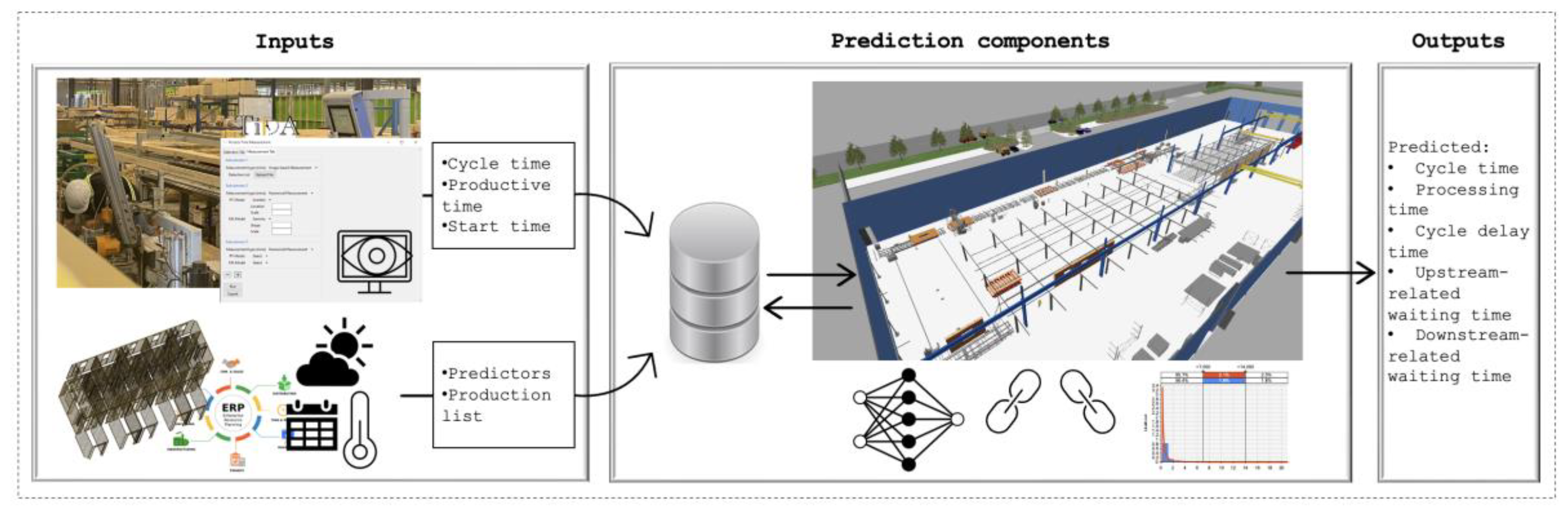
Figure 2.
A portion of the wall production line.
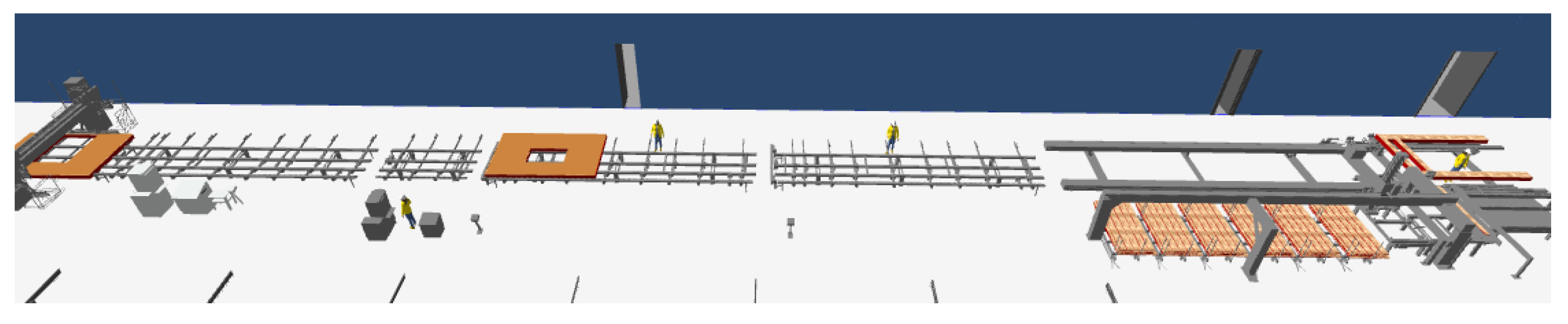
Figure 3.
(a) Stop signs unblocked; (b) stop signs blocked [2].
Figure 3.
(a) Stop signs unblocked; (b) stop signs blocked [2].
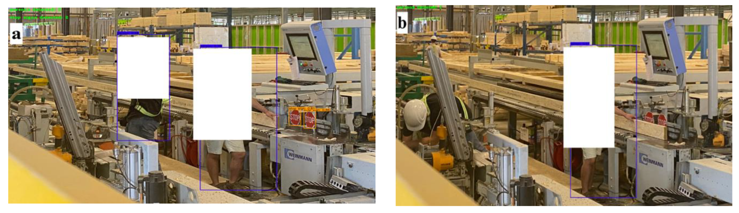
Figure 6.
3D model of the factory.
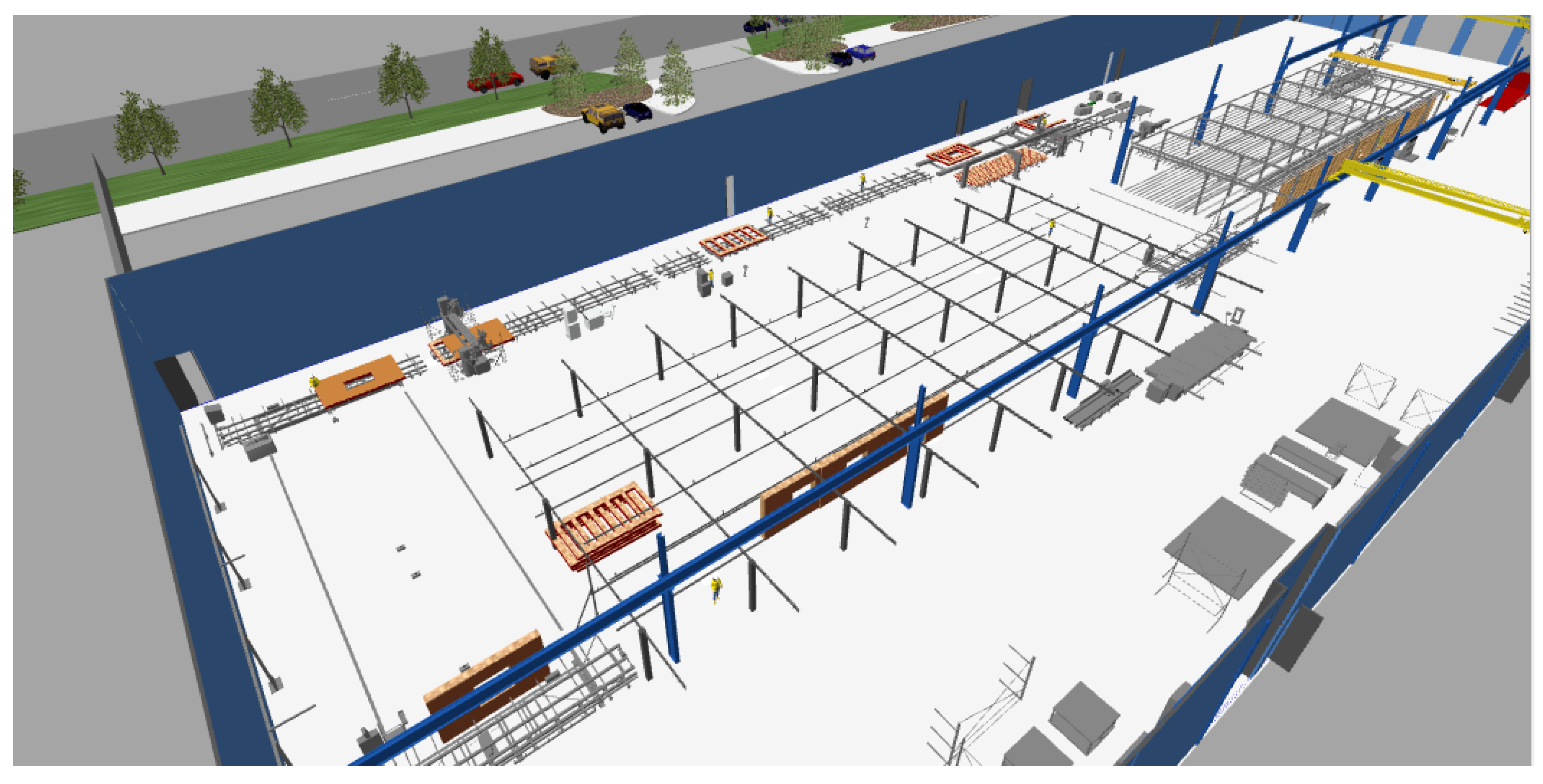
Figure 8.
of the NN model versus that of the LR model.
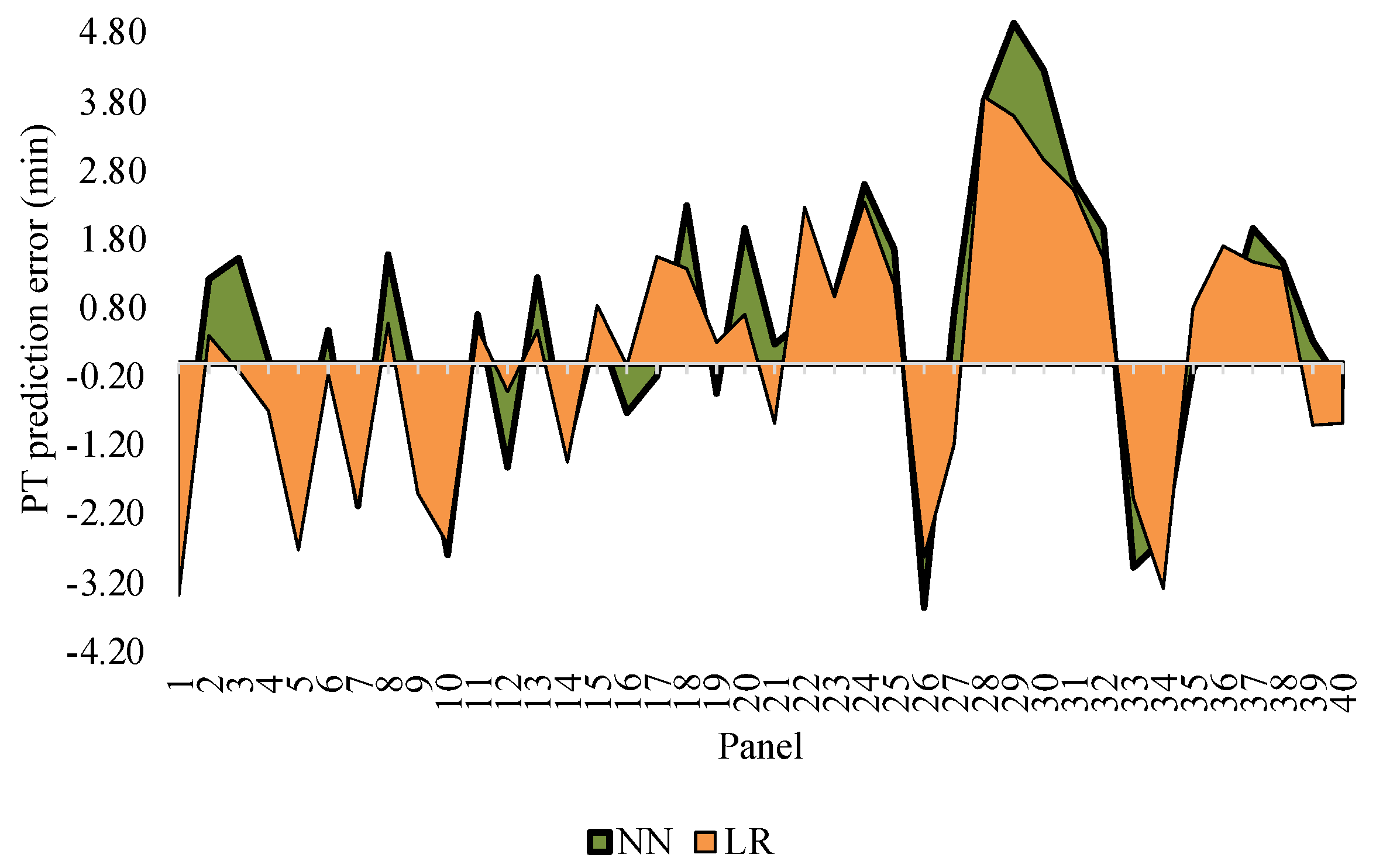
Table 4.
Evaluation results for PT predictions.
| Actual PT (min) | NN | LR | RF | Fixed rate | |||||
|---|---|---|---|---|---|---|---|---|---|
| Predicted PT (min) | (min) | Predicted PT (min) | (min) | Predicted PT (min) | (min) | Predicted PT (min) | (min) | ||
| 1 | 14.17 | 11.95 | −2.22 | 10.78 | −3.39 | 11.36 | −2.81 | 7.33 | −6.84 |
| 2 | 10.58 | 11.79 | 1.21 | 10.98 | 0.40 | 10.82 | 0.24 | 8.61 | −1.97 |
| 3 | 8.83 | 10.34 | 1.51 | 8.71 | −0.12 | 9.81 | 0.98 | 6.83 | −2.00 |
| 4 | 9.92 | 10.00 | 0.08 | 9.23 | −0.69 | 11.14 | 1.22 | 8.03 | −1.89 |
| 5 | 15.17 | 13.75 | −1.42 | 12.45 | −2.72 | 11.40 | −3.77 | 5.31 | −9.86 |
| 6 | 4.58 | 5.05 | 0.47 | 4.42 | −0.16 | 5.95 | 1.37 | 4.39 | −0.19 |
| ... | ... | ... | ... | ... | ... | ... | ... | ... | |
| 38 | 7.42 | 8.90 | 1.48 | 8.79 | 1.37 | 8.78 | 1.36 | 8.13 | 0.71 |
| 39 | 12.67 | 12.99 | 0.32 | 11.77 | −0.90 | 11.08 | −1.59 | 8.71 | −3.96 |
| 40 | 11.33 | 11.00 | −0.33 | 10.46 | −0.87 | 9.83 | −1.50 | 7.77 | −3.56 |
| MAE (min) | 1.57 | 1.52 | 1.81 | 2.87 | |||||
| MPE | 19% | 19% | 21% | 29% | |||||
| SE (min) | 17.68 | 5.62 | 10.01 | −98.64 | |||||
Table 5.
Evaluation results for CT predictions.
| Actual CT (min) | Prediction system | Fixed rate | |||
|---|---|---|---|---|---|
| Predicted CT (min) | (min) | Predicted CT (min) | (min) | ||
| 1 | 22.02 | 15.21 | −6.81 | 8.62 | −13.40 |
| 2 | 11.5 | 12.06 | 0.56 | 10.12 | −1.38 |
| 3 | 8.9 | 10.66 | 1.76 | 8.04 | −0.86 |
| 4 | 10 | 10.68 | 0.68 | 9.44 | −0.56 |
| 5 | 17.63 | 14.62 | −3.01 | 6.25 | −11.38 |
| 6 | 7.57 | 7.64 | 0.07 | 5.16 | −2.41 |
| ... | ... | ... | ... | ... | |
| 38 | 7.82 | 10.38 | 2.56 | 9.56 | 1.74 |
| 39 | 18.67 | 14.61 | −4.06 | 10.25 | −8.42 |
| 40 | 14.8 | 12.18 | −2.62 | 9.14 | −5.66 |
| MAE (min) | 3.03 | 4.72 | |||
| MPE | 23% | 34% | |||
| SE (min) | −50.10 | −156.25 | |||
Disclaimer/Publisher’s Note: The statements, opinions and data contained in all publications are solely those of the individual author(s) and contributor(s) and not of MDPI and/or the editor(s). MDPI and/or the editor(s) disclaim responsibility for any injury to people or property resulting from any ideas, methods, instructions or products referred to in the content. |
© 2023 by the authors. Licensee MDPI, Basel, Switzerland. This article is an open access article distributed under the terms and conditions of the Creative Commons Attribution (CC BY) license (http://creativecommons.org/licenses/by/4.0/).
Copyright: This open access article is published under a Creative Commons CC BY 4.0 license, which permit the free download, distribution, and reuse, provided that the author and preprint are cited in any reuse.


