
Submitted:
30 April 2024
Posted:
01 May 2024
You are already at the latest version
Abstract
To understand dynamics in climate change, informing policy decisions and prompting timely action to mitigate its impact, this study provides a comprehensive analysis of the short-term trend of year-on-year CO2 emission changes across ten countries, considering a broad range of factors including socioeconomic, CO2-related industry, and education. This study uniquely goes beyond the common country-based analysis, offering a broader understanding of the interconnected impact of CO2 emissions across countries. Our preliminary regression analysis, using the ten most significant features, could only explain 66% of variations in the target. To capture emissions trend variation, we categorized countries by the change in CO2 emission volatility (high, moderate, low with upward or downward trends), assessed using standard deviation. We employed machine learning techniques, including feature importance analysis, Partial Dependence Plots (PDPs), sensitivity analysis, and Pearson and Canonical correlation analyses, to identify influential factors driving these short-term changes. The Decision Tree Classifier was the most accurate model, with an accuracy of 96%. It revealed population size, CO2 emissions from coal, the three-year average change in CO2 emissions, GDP, CO2 emissions from oil, education level (incomplete primary), and contribution to temperature rise as the most significant predictors, in order of importance. Furthermore, this study estimates the likelihood of a country transitioning to a higher emission category. Our findings provide valuable insights into the temporal dynamics of factors influencing CO2 emissions changes, contributing to global efforts to address climate change
Keywords:
Absolute change in CO2 emissions
; Short-term trend analysis
; Machine learning
1. Introduction
Greenhouse gases (GHG) are one of the main reasons behind natural disaster risks. Combined with socio-economic conditions, governance, and conflict, these complex and dynamic phenomenon are causing huge damages [1]. Extensive research has been conducted on natural disaster risks related topic and their possible implications, resulting in the establishment of several indicators suitable to explain and quantify their significance and possible impact [2,3,4]. While research have illuminated various aspects of disaster risks, contributing thus to the progress achieved in this field, the current frameworks designed to reduce their impacts are often designed for long-term durations [3], which represents a major constraint, considering the capricious nature of these hazards and their escalating repercussions on human lives. Furthermore, even when those frameworks are implemented, the persistence of peril persists, thereby increasing the vulnerability of nations categorized as least developed [5], limiting those nations to ameliorate their positions. As a fact, considering the WRI and its subcomponents, it is more likely for a country, either developed or not, to remain in its position of vulnerability and susceptibility within five consecutive years. Also, least developed countries have only 1 percent of probability to improve their position, but only after 5 years [6]. Among GHG, Carbon dioxide (CO2), receives particular attention due to its high production from human activities and its negative environmental impact such as air pollution, temperature rise, etc. this situation is alarming since least developed countries which pollute and emit less are more exposed to disasters induced by the production of CO2 compared to developed countries which pollute and emit the most [7]. Thanks to the technological advances, several studies have provided accurate forecasting and projections of CO2 emissions, deep insight on the interplay of other components such as political, geographical, economic, environmental, societal to their production, thus enhancing our understanding on the subject which support current frameworks such as the Paris Agreement and other decarbonization pathways. Understanding factors contributing to CO2 emissions, whether they are direct (like burning fossil fuels) or indirect (like deforestation), can be relatively straightforward; however, explaining the changes in CO2 emissions over a period is a more complex task because such process involves not only understanding the factors contributing to emissions, but also understanding their dynamics over time. Such process requires a deep understanding of a wide range of fields, including technological, economic, and policy changes, as well as changes in energy use, land use, and population growth. Moreover, the relationship between these factors and CO2 emissions can be non-linear and involve complex feedback loops. For example, economic growth might lead to increased energy use and CO2 emissions, but it could also drive technological innovation that reduces emissions[8,9]. This subject is even more complex considering the possible implication of decarbonization on the economy of nations which, in majority are sustained by high CO2 emitters such as coal, oil, cement. The limited or absent clear responses to explain the change CO2 emissions over time and on a global scale, coupled with the urgent need to provide a more inclusive response to address this threat, induce this research which aims to answer these questions:
- How do overtime, economic, CO2 related industries, educational levels and population dynamics interacted to influence the short-term trend change in CO2 emissions across diverse countries having diverse characteristics with respect of the factors mentioned?
- Which insight in term of identification and quantification of the temporal dynamics and influence of these factors can machine learning techniques highlight to deepen one’s understanding on this change overtime on a global scale?
This study addresses a critical gap in CO2 emissions research. While existing studies often focus on individual countries with limited factors, this approach hinders a comprehensive global understanding. By analyzing a broader set of factors across diverse countries, our research sheds light on the complex dynamics driving changes in CO2 emissions. This deeper understanding is crucial for formulating effective global responses to this pressing environmental hazard.
By leveraging a unique dataset that combines data for 10 different countries having different characteristics, this research acknowledges both direct and indirect factors previously identified by experts and researchers in the field as having a potential impact on changes in CO2 emissions. Machine learning techniques and statistical techniques are employed to understand their temporal dependency and contribution to the change in CO2 emissions. By doing so, a clear and quantifiable understanding of the unique interplay and contribution of these factors to the change in CO2 emissions on a global scale will replace the blurred comprehension. Furthermore, the outcome of this research will instill a sense of generalizability of these results, considering the diverse backgrounds of the countries selected.
To achieve this task, the remainder of the paper is organized as follows: after the first section dedicated to the introduction, the second section will discuss about the materials and methods considered, followed by the results and discussions section. Finally, the last section is for the conclusion.
2. Materials and Methods
2.1. Data Collection
From 1960 to 2022, 26 datasets from 10 countries were combined to create a unique (Appendix A). These countries were considered based on their economic level, population dynamics, regional location, education level and their contribution to CO2 emissions. Namely, the United States, United Kingdom, South Korea, China, India, France, Brazil, Democratic Republic of Congo, Nigeria, and South Africa were used as target countries. Two reputable platforms were considered for data collection: ourworldindata.org and the world bank open data. Appendix 1 presents each dataset, here considered as features of the final dataset. Organized on a yearly base timing, the dataset combines 5 groups of features: Population dynamics (2), Economic (3), Education (7), CO2 emissions related industry (5), CO2 related emissions and temperature (7). Missing values were imputed using the Iterative Imputation technique from the Fancy impute of Python (Appendix B)
2.2. Data Preparation
Using python 3.10 on the last distribution of anaconda, was achieved using the supervised machine learning technique (both regression and classification). Considering the varying trend for each country of the Absolute change in CO2 emissions (Appendix D) which is the target variable, it was necessary to mitigate this considering its potential negative impact on the performance of the algorithms. To capture the short-term trend of the target, countries were grouped based on the percentile of volatility of the mean value for 3 years of the target. This data-driven approach instills generalizability of the findings and helped overcome the limitation of the regression technique which suffers from the extreme variability of the target.
Figure 2 explains the grouping process.
After grouping data by country, a rolling period of 3 was define on the target to obtain the mean value for 3 years for each country which is the new target. By the same process of grouping data by country, the standard deviation was determined for each of them. The percentiles (25% as moderate low threshold and 75% as moderate high threshold) were used as thresholds to define the low, moderate and high volatility in the 3 years mean values for each country. This stage helped to categorize each countries’ variation in a more data driven-driven approach that can be adapted to other datasets. Considering that the standard deviation is always positive but the variations sometimes take negative values, it was imperative to specify the direction of the variation as either negative or positive. Thus, after verification of the sign of the of the new target, that sign was picked and assigned to the level of volatility defined by the threshold. This process resulted in six classes of volatility: High positive and negative, Moderate positive and negative, and Low positive and negative. By doing so, not only the volatility is defined but also the direction making it more comprehensive for the interpretation of the prediction. The outcome of this process is presented in the result section.
2.3. Machine Learning Algorithms
For the regressions approach, the performance of following regressors was compared: Linear Regression[10], Ridge Regression[11], Bagging Regressor[12], Random Forest Regressor[13], Gradient Boosting Regressor[14], XGBoost Regressor[15], AdaBoost Regressor [16] and KNeighbors Regressor [17] . Concerning classification, the performance of the following classifiers was compared: Logistic Regression (LogReg)[18], Decision Tree (DT)[19], Random Forest Classifier (RF)[20], XGBoost classifier (XGB)[21], Multi-Layer Perceptron classifier (MLP)[13], Bagging (BC)[22], AdaBoost (ABC)[23], Gradient Boosting (GB)[24], Support Vector (SVC)[25], Gaussian Naïve Bayes (GNB)[26].
2.4. Metrics
Two rounds of evaluation were considered in the two approaches: the first consisting in the selection of the best performing model and the second in the final evaluation of the best performing model. To achieve this, the following metrics were considered:
- ○
- For the selection of the best performing algorithm:
- ●
- ▪
- ○
- For final evaluation:
- ●
- Regression: Mean squared error, Residuals, R-squared
- ▪
- Classification: Accuracy score, Mathhew correlation coefficient, Confusion matrix and classification report.
2.5. Explainable Machine Learning Techniques
To instill confidence to the prediction, the following explainable techniques were considered:
2.5.1. Partial Dependence Plots (PDPs):
It provides plots showing the marginal effect that features have on the predicted outcome of a machine learning model. A PDP can show whether the relationship between the feature and target is complex, monotonic or linear. It is an important technique since it has a causal interpretation, which means that is explains the outcome of a prediction [34,35].
It is defined as:
where:
xs are the features for which the PDP is to be plotted
xc are the other features used in the machine learning model f
xc(i) are the actual features in the model which we are not interested, and
n is the number of instances in the dataset.
This analysis was achieved using the PartialDependenceDisplay package from the sklearn library. The outcome of this analysis is presented in the result section.
2.5.2. Sensitivity Analysis
A useful technique to understand the impact of changes in the input features to the model outcome. By doing so, it provides insight into the most important features by quantifying the uncertainty in the model’s output[36]. It is often used to measure the correlation between changes in an input variable and the resulting changes in the output variable and aims to study how the uncertainty in the output can be allocated to different sources of uncertainty in the inputs[37]. This process can be represented as follows:
Considering a model as a function , where N is the number of input variables and M the number of output variables. The input variables are represented as a vector , and the output variables are represented as a vector . The model maps the input variables to the output variables, for instance, y = g(x).
For a given input variable , the sensitivity of the output variable with respect to can be calculated as follows:
Formula (2), represents the relative change in for a relative change in .
This analysis was achieved using the saltelli from SALib package for sample generation following the defined problem and sobol from the same SALib to get the first and total order sensitivity indices. The result of this process is provided in the result section.
2.5.3. Feature Analysis
A correlation analysis, especially, the Pearson Correlation between features and the Canonical Correlation[38] among groups of features were considered to evaluate the interplay of the features overtime, to complete the one achieved using PDPs and Sensitivity analysis.
2.6. Research Design
The process followed in this research is represented in Figure 3.
Once the data is collected from the different sources and for the considered country, they are merged to make a unique dataset. Missing values are imputed using the iterative imputation, then, grouped by country before applying a temporal splitting of the train from 1960-12-31 to 2009-12-31 and test from 2010-12-31 to 2022-12-31. Features were scaled using the Standard Scaler from the sklearn library. The Pearson and Canonical correlation analysis took place for the analysis of the interplay of features. The first approach of the modeling consisted in the regression technique to predict the mean value for 3 years of the of the absolute change in CO2 emissions, variable which could capture the short-term trend of the target. Iteratively, the baseline modelling and grouping by volatility was considered for improvement since the other did not improve it. The poor performance resulting from this approach led to consider the classification technique. To achieve this, the process explained in Figure 3 was applied on the new target. And to improve the performance of the classifiers class balancing techniques such as SMOTE, ADASYN and class weight were considered. After this stage, the XAI is achieved and the result including the one resulting from the correlation analysis was analyzed and interpreted.
3. Results
3.1. Regression Analysis
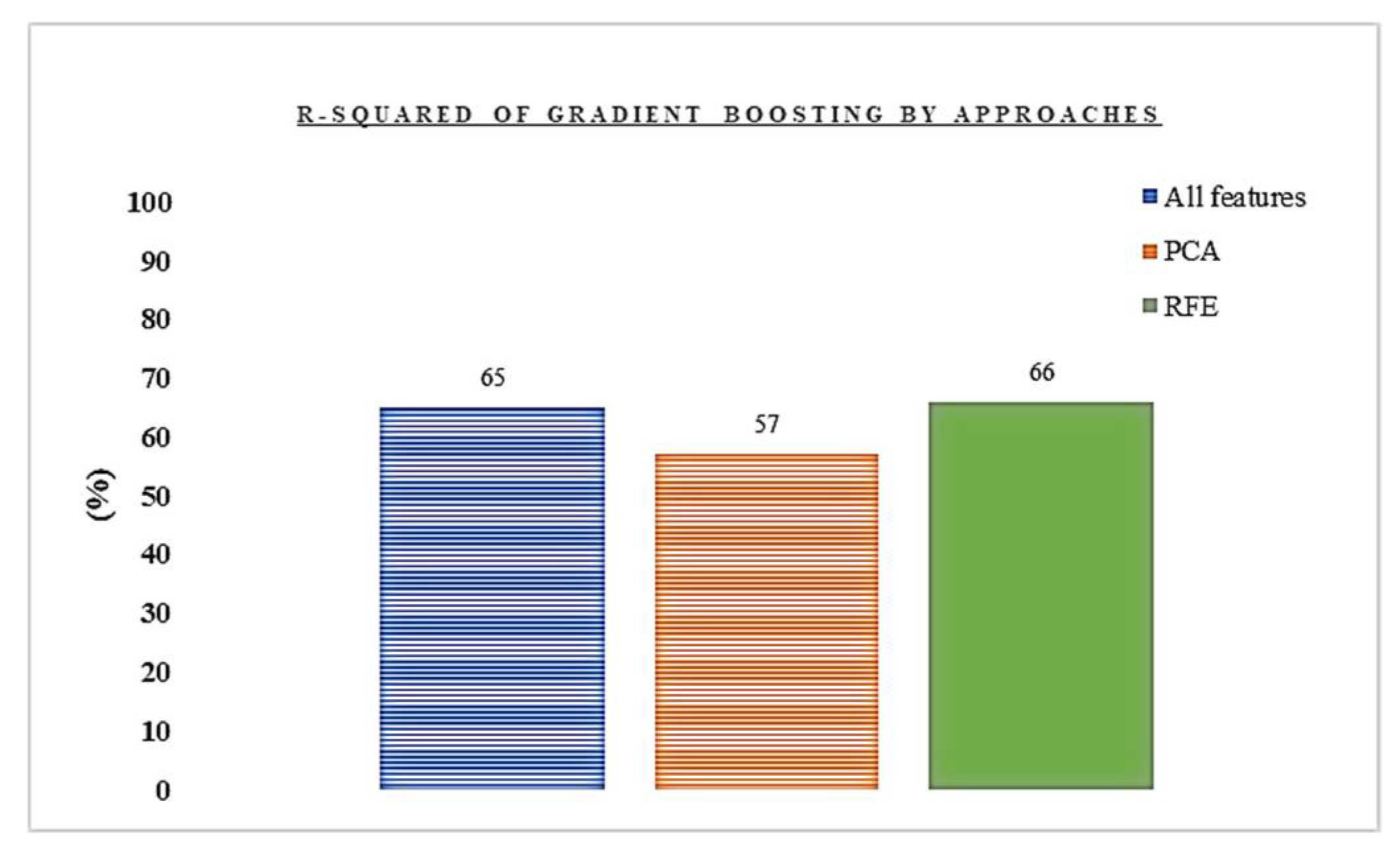
In the process of the selection of the best regressor, it appeared that the Gradient Boosting Regressor algorithm provided the best score (Figure 4, appendix C1, C2, C3). To improve its performance, the reduction of dimension was applied using the PCA and feature selection techniques (Figure 5).
Figure 4.
Comparison of r-squared by model.
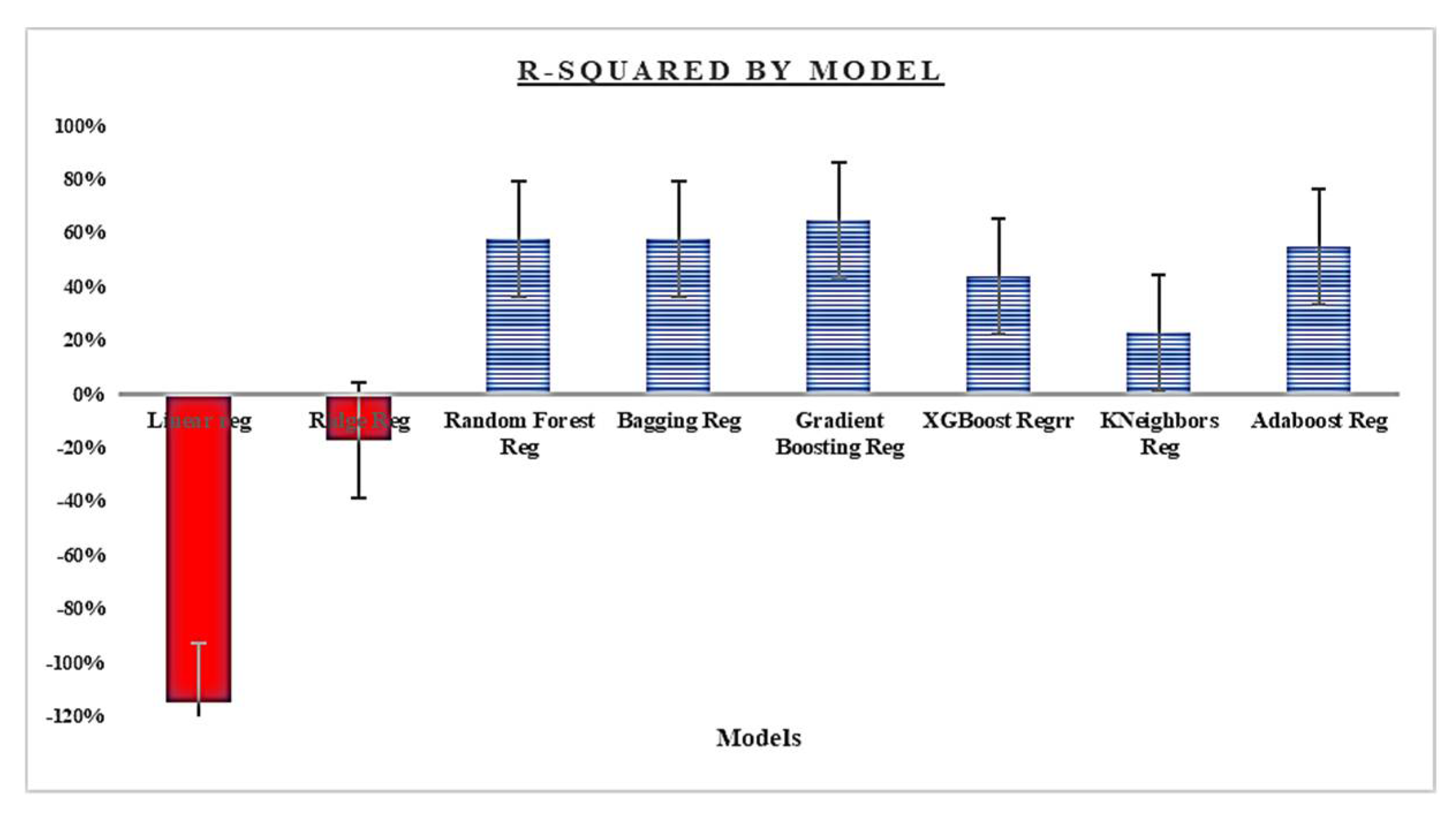
This general poor performance led to consider the option of grouping the target based on each country’s volatility to mitigate that difference which potentially tends to reduce the effectiveness of the model to capture hidden patterns during the training. Figure 6 summarizes the result of this approach. Having the Gradient Boosting Regressor as the best model, PCA (using n_components of 0.98) and selection of the best 10 features using the Recursive Feature Elimination (RFE) [39] with the best model were applied. These best features are: co2 from cement, co2 from gas, co2 from coal, share of cumulative co2 emissions, Population-Education: Incomplete Primary, Population (number), GDP per capita, change in gdp, Annual co2 emissions growth (%) and Absolute co2 change.
Figure 5.
Comparison of r-squared by feature approaches.
This approach provided two groups: high volatility (China and United States) and low volatility (the remaining countries). In applying the same process of model selection, there is an observed improvement for countries in the low category considering the result of the AdaBoost Regressor (70 % r-squared) despite its inefficiency in generalizing the test set (cross validation score: -0.89).
Figure 6.
Comparison of r-squared by volatility group.
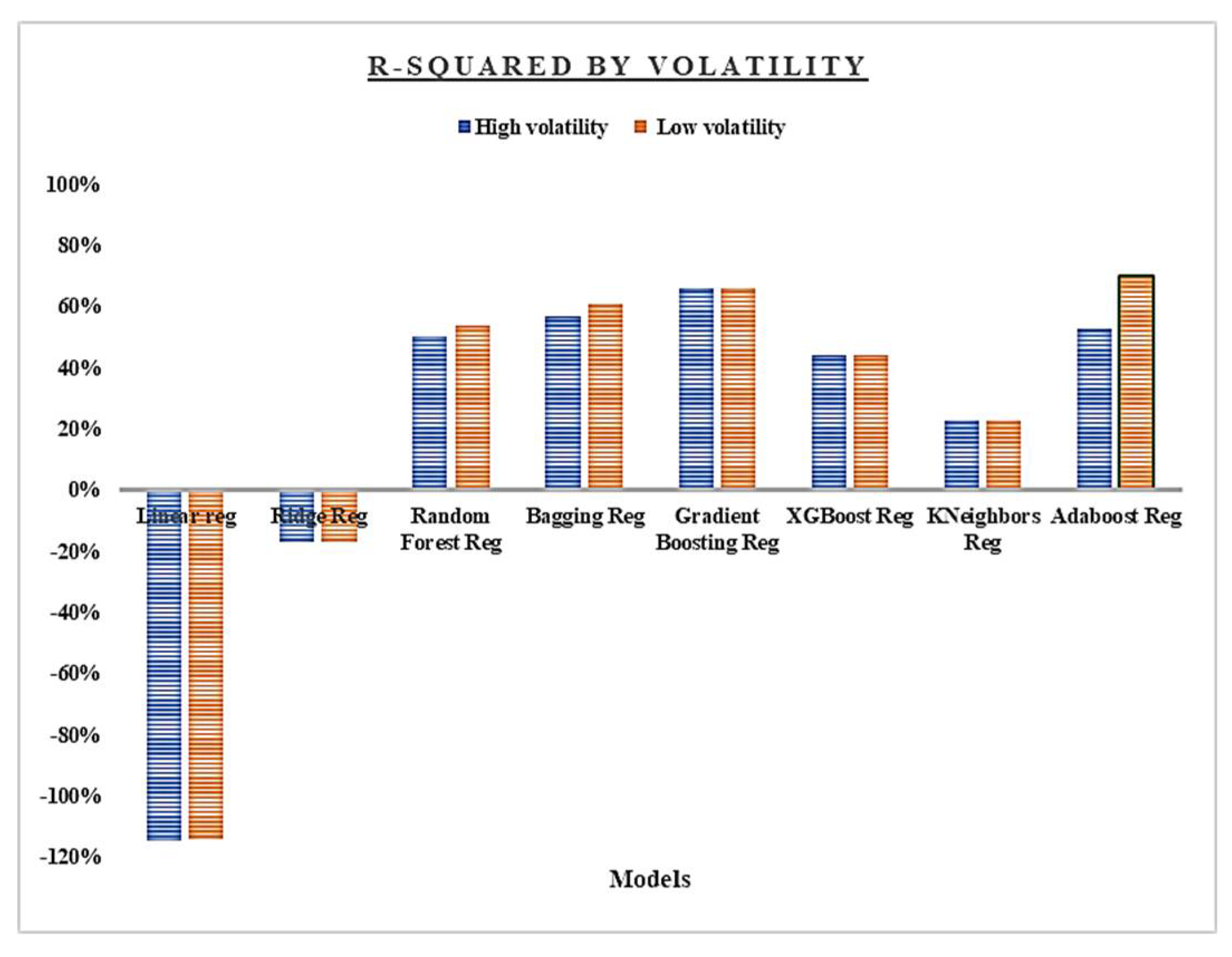
Overall, using regression appeared not to be suitable since it is inappropriate to capture the hidden pattern in the dataset which is major a prerequisite for further investigation. This limitation justifies the need to find alternatives, among which, grouping the short-term trend in classes following the process presented in Figure 2
3.2. Classification Analysis
3.2.1. Grouping Target in Classes
The process explained in Figure 2, could provide 6 imbalanced classes presented in Table 1 and Figure 7. A better understanding of this classification is provided in Figure 5 which depicts the temporal dynamics of the mean value for 3 years for each country.
High (positive and negative) category represents the group of high polluting countries despite efforts to reduce the level of CO2 emissions over time. Moderate (positive and negative) category is the group of emitters whose level of CO2 emissions is important but still tolerable compared to the previous group. And the low (positive and negative) is those countries whose emission is quite good compared to the others. It appears, over time, that countries belonging to a given category remained in it but experienced the two directions (positive or negative) (Table 2), except India, which in the early 2000’s moved from the moderate to high volatility group (Figure 8).
For each class, Figure 9 presents their occurence overtime
Figure 6 demonstrates that the positive trend occurred almost every year, making their number higher than the negatives in each category. This trend confirms the general increase in CO2 emissions worldwide despite efforts to reduce it. Having this categorization done, the performance of the classifiers applied on this data is provided in Table 3.
The performance of the selected classifiers, using the baseline architecture, is provided in Table 5.
It appears that the Decision Tree model performed better compared to the other classifiers. Even after search of the best parameters, the confusion matrix as well as the classification report of the DT present error in prediction of one instance out of 19 from class moderate positive (providing a recall of 0.95, precision of 1.00 and a f1 score of 0.97) which is predicted as low positive, 5 instance out of 33 from class moderate negative (having a recall of 0.85, precision of 0.97 and f1 score of 0.97) predicted as high negative, and one instance out of 16 from class high positive (displaying a recall of 0.94, precision of 1.00 and f1 score of 0.97) predicted as moderate negative.

Table 3.
Confusion matrix and classification report.
| Confusion matrix | Precision | Recall | F1-score | Support | ||||||
|---|---|---|---|---|---|---|---|---|---|---|
| High negative | 12 | 0 | 0 | 0 | 0 | 0 | 0.71 | 1.00 | 0.83 | 12 |
| High positive | 0 | 27 | 0 | 0 | 0 | 0 | 1.00 | 1.00 | 1.00 | 27 |
| Low negative | 0 | 0 | 15 | 0 | 1 | 0 | 1.00 | 0.94 | 0.97 | 16 |
| Low positive | 0 | 0 | 0 | 23 | 0 | 0 | 0.96 | 1.00 | 0.98 | 23 |
| Moderate negative | 5 | 0 | 0 | 0 | 28 | 0 | 0.97 | 0.85 | 0.90 | 33 |
| Moderate positive | 0 | 0 | 0 | 1 | 0 | 18 | 1.00 | 0.95 | 0.97 | 19 |
| High negative | High positive | Low negative | Low positive | Moderate negative | Moderate positive | |||||
Based on this result and despite the small misclassification, the model could capture the general short-term trend (3 years average) of the target. The features contributing to this prediction are used to understand their interplay and contribution over time on the target.
3.3. Feature Analysis
3.3.1. Feature Importance Analysis
Using the decision tree algorithm after a grid search of the best parameters, this analysis reveals that 8 features contribute to the prediction (Figure 10).
From the present group of features, two features from the economic group (change in gdp and gdp per capita), one from the population group (Population number), one from education group (Population-Education: Incomplete Primary), one from CO2 related industry (CO2 from oil), and the remaining three from CO2 related activity (GHG by world region, share of cumulative co2 emissions and the mean value of 3 years) contributed to the prediction. A summary of the PDPs (Table 4) summarizes the direction of their contribution.
A close look at each country's trend over time for the features considered (Figure 11) provides a better understanding of the overall dynamics.
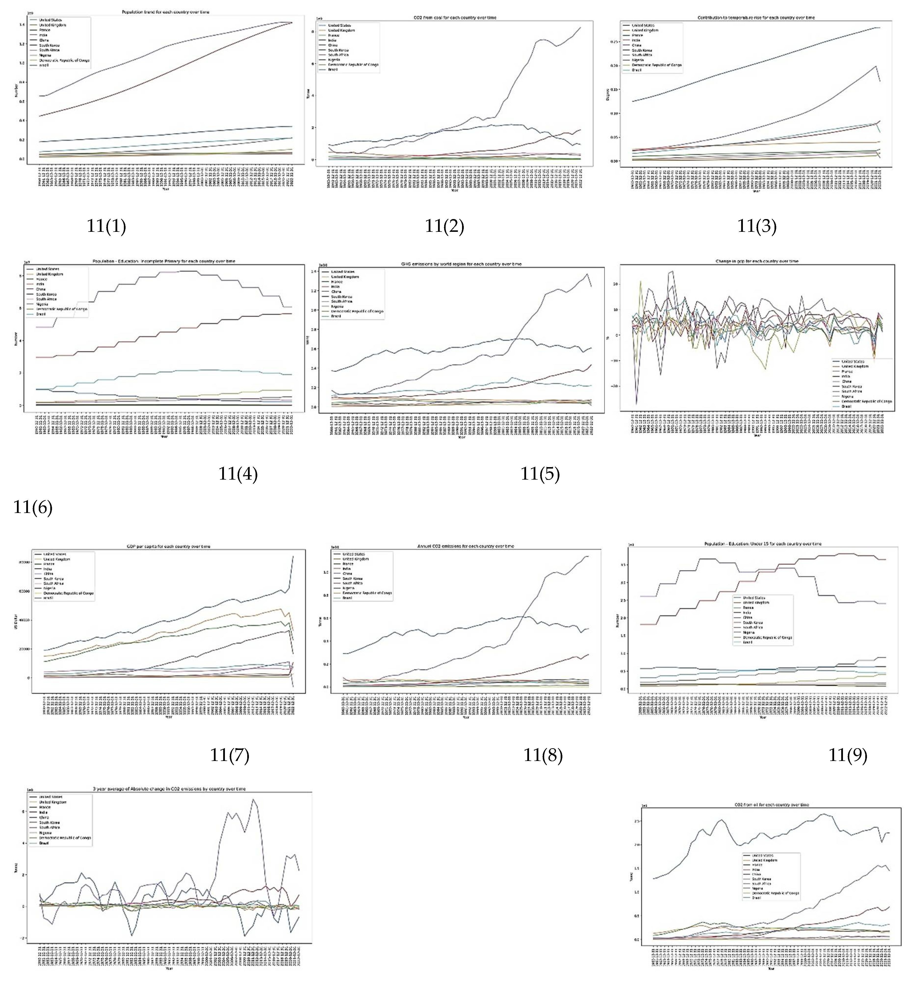
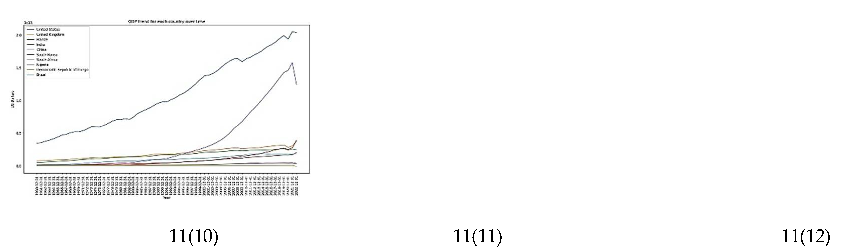
In all the categories, the increase or decrease in the 3 years average determines the sign (positive or negative) of the category [11(10)]. Coupled with the fluctuation in the 3 years average, the dynamics in the population number influences the categorization of a country. High emitters have a large population compared to others [11[(1)]. Over time, countries having an important variation in the change of gdp tend to emit less compared to those having low variations [11(6)]. The trend of the gdp per capita [8(6)] coupled with the gdp [11(12)] suggests that they cannot clearly explain the trend in CO2 emissions since some rich countries emit less compared to others. It also appears that the level of education [11(4 & 9)], most specifically, early access to education could potentially explain the target. Indeed, in the group of countries considered, the wealthier a country is, the number of children having early access to education increases also. These results demonstrate possible interaction among features, which, once understood, could deepen our understanding of the present dynamics. To capture possible dependency between features, which could not be achieved using the feature importance and PDPs which assumes independence among features, the sensitivity analysis was applied.
3.3.2. Sensitivity Analysis
Using 1000 samples with a bounds between -5 and 9, it appears that seven variables 7 variables, slightly different than those from the feature important analysis, have impact on the performance of the model (Figure 12)
In capturing possible interactions among features, this analysis could identify and quantify four key groups that contribute to the short-term dynamics of year-on-year changes in CO2 emissions. These groups are population, CO2 related industries (including coal and oil), economic activity assessed through the GPD, the contribution to temperature rise associated CO2 emissions and early access to education assessed by the Population-Education: Incomplete Primary. These features could be grouped into two: those having a direct impact (Population, CO2 from coil, oil, mean-3y), and those which can explain it indirectly (GDP, contribution to temperature rise and Population-Education: Incomplete Primary).
3.3.3. Correlation Analysis
To deepen understanding on the interaction of features, the Pearson and Canonical correlation were used. Figure 13 provides the correlation table of the features in the dataset.
In comparing the group of features, there is a strong positive correlation among variables in the CO2 emissions and CO2 related industry with the group related to the level of education, economic features, population number, but not with the population growth rate or GDP per capita. In more details, there is a strong positive correlation (>= 0.50) between the annual CO2 emissions and GDP (0.84), Population number (0.55), Population – Education: Lower Primary (0.50), Population -Education: Lower Secondary (0.71), Population -Education: Upper Secondary (0.82), Population -Education: Post Secondary (0.86), Contribution to temperature rise (0.86), Share of cumulative CO2 emissions (0.71), Cumulative CO2 emissions (0.85), CO2 from coal (0.92), CO2 from oil (0.84), CO2 from gas (0.73), CO2 cement (0.77), GHG emissions by world region (0.98); there is also a strong negative correlation between this same variable and the Population growth rate (-0.37). This result confirms the existing studies about the interplay of the considered variables to the emission of CO2. For instance, rich countries are high polluters, and the concentration of population is one reason behind CO2emissions fluctuations. Also, education plays an important role in understanding and developing ways to mitigate CO2 emissions[8]. While such observation seems straightforward, it is not the case for the Absolute change in CO2 emissions which is the target variable. Indeed, only Population – Education: Primary (0.53 / 0.63), Population – Education: Lower Secondary (0.6 / 0.72), CO2 from coal (0.57 / 0.70) and CO2 from cement (0.56 / 0.69) have a strong positive correlation with the target. On the short-term, we can observe an average increase of 1.26% in the correlation coefficient between CO2 related features with the target, as well as in the education features and population number in comparison to what it was with the Absolute change in CO2 emissions. Thanks to the Canonical correlation, it is possible to deeply visualize this correlation direction. However, when it comes to the corresponding categories, this direction is still strong, but changes to the negative. This suggests that as the value increases, it is more likely for the target to be in the high positive category. To deepen understanding on the interplay of features already provided by the sensitivity analysis, the canonical correlation analysis allows, through plotting, to visualize the direction of these features over time. To achieve this, after grouping features based on their groups, a comparison between them was achieved in the following order: Population with co2 industry, Population with CO2 related emissions, Population with education, population with economy, CO2 industry with CO2 related emissions, CO2industry with education, CO2 related emissions education, CO2 industry with economy, CO2 related emissions with economy, education with economy. The group of Figure 10 presents the result of this analysis.
Figure 14.
Canonical correlation: coefficient plot.
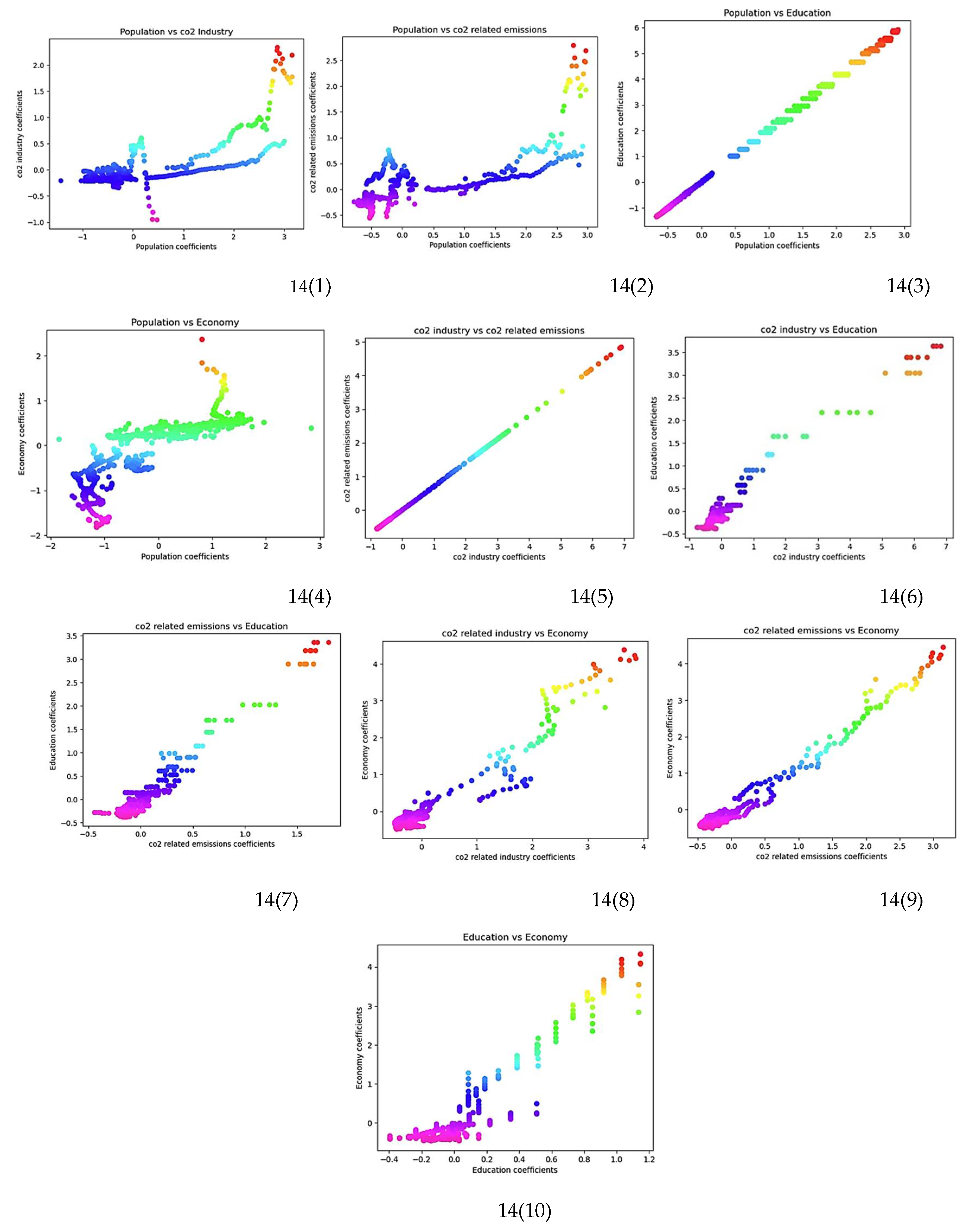
Two trends are displayed from this analysis. Over time, there is a linear trend in the group of CO2 related emissions and industry with education [14(6), 10(7)], and economy [14(8), 14(9)], population with education [14(3)], and education with economy [10(10)], and nonlinear one for population with CO2 related emissions and industry [14(1), 14(2)] and population with economy [14(4)]. In the group of countries considered, regardless of the decreasing trend in population growth rate of some countries, this analysis unveils that the dynamics in the population affect differently each country’s economy. As it grows, it tends to positively impact the CO2 emissions, influencing by this, the short-term variations of CO2 emissions. Early access to education is displaying a linear trend with the economy growth, CO2 emissions and population dynamics suggesting that the more a country emits, the more it becomes wealthy and could implement laws to support education. The level of education increases with growth of the economy and CO2 emissions. The contribution to temperature rise does not solely depend on the emissions of CO2. However, as for the early access to education, this indicator is meaningful to explain the target of this analysis. These trends could help anticipate future dynamics in the monitoring of CO2 emissions resulting in the implementation of adequate policy to tackle this threat while maintaining a good level of economy.
3.4. Discussion
A close look at some statistics of the categories provided in Table 5, coupled with the sensitivity analysis result suggest that:
Table 5.
Summary of mean values by features in each category.
| Features | High negative | High positive | Moderate negative | Moderate positive | Low negative | Low positive |
| Population (number) | 4.81E+08 | 8.07E+08 | 7.18E+07 | 7.91E+07 | 6.74E+07 | 6.74E+07 |
| CO2 from coal | 1.45E+09 | 1.76E+09 | 1.15E+08 | 1.24E+08 | 1.04E+08 | 8.21E+07 |
| Mean-3y | -7.31E+07 | 1.07E+08 | -1.07E+07 | 1.06E+07 | -3.02E+06 | 4.76E+06 |
| GDP | 9.99E+12 | 4.27E+12 | 1.96E+12 | 9.79E+11 | 1.72E+11 | 1.38E+11 |
| CO2 from oil | 1.58E+09 | 8.85E+08 | 2.12E+08 | 1.71E+08 | 2.43E+07 | 2.31E+07 |
| Population-Education: Incomplete Primary | 2.04E+07 | 4.32E+07 | 2.10E+06 | 5.82E+06 | 3.90E+06 | 3.94E+06 |
| Contribution to temperature rise | 0.173045 | 0.098758 | 0.029083 | 0.022507 | 0.010212 | 0.008529 |
- a.
- High Negative: Countries in this group have a high average population and GDP, a high CO2 emission from both coal and oil. Despite their high GDP and CO2 emissions, these countries have seen a decrease in CO2 emissions over time. However, they also have a high contribution to temperature rise.
- b.
- High Positive: Countries in this group also have a high average population, a slightly lower GDP compared to the High Negative group and they have seen an increase in CO2 emissions over time. Surprisingly, they have a lower contribution to temperature rise compared to the High Negative group. This could be due to their past contribution.
- c.
- Low Negative: Countries in this group have a lower average population and GDP compared to the High groups. They have lower CO2 emissions from both coal and oil and have seen a decrease in CO2 emissions over time. Finally, they contribute less to temperature rise compared to the High groups.
- d.
- Low Positive: Countries in this group have a similar average population to the Low Negative group. They have a lower GDP compared to the Low Negative group but they have seen an increase in CO2 emissions over time. They also contribute less to temperature rise compared to the High groups.
- e.
- Moderate Negative: Countries in this group have a moderate average population and GDP. They have moderate CO2 emissions from both coal and oil, and they have seen a decrease in CO2 emissions over time. They contributed moderately to temperature rise compared to the High groups.
- f.
- Moderate Positive: Countries in this group have a similar average population to the Moderate Negative group. They have a lower GDP compared to the Moderate Negative group and they have seen an increase in CO2 emissions over time. They have a lower contribution to temperature rise compared to the Moderate Negative group.
- ●
- A comparison of the two categories, High negative and High positive, suggests that:
- ●
- Population (number): The average population is higher in the High positive group (approximately 807 million) compared to the High negative group (approximately 481 million). This suggests that countries with larger populations tend to have increasing CO2 emissions.
- ●
- CO2 emissions from Coal: Both groups have high CO2 emissions from coal, but the High positive group has slightly higher emissions on average (approximately 1.76 billion tonnes) compared to the High negative group (approximately 1.45 billion tonnes).
- ●
- CO2 emissions from Oil: The High negative group has higher CO2 emissions from oil (approximately 1.58 billion tonnes) compared to the High positive group (approximately 885 million tonnes).
- ●
- 3-Year Mean Change in CO2 emissions (Mean-3y): The High negative group shows a decrease in CO2 emissions over time (average change of -73 million tonnes), while the High positive group shows an increase (average change of 107 million tonnes).
- ●
- GDP: is higher on average in the High negative group (approximately 9.99 trillion USD) compared to the High positive group (approximately 4.27 trillion USD). This suggests that wealthier countries tend to have decreasing CO2 emissions.
- ●
- Population with Incomplete Primary Education: The High positive group has a higher average population with incomplete primary education (approximately 43.2 million) compared to the High negative group (approximately 20.4 million).
- ●
- Contribution to Temperature Rise: The High negative group has a higher average contribution to temperature rise (0.173) compared to the High positive group (0.099).
The High negative group tends to have wealthier countries with larger CO2 emissions from oil and a larger contribution to temperature rise. On the other hand, the High positive group tends to have countries with larger populations, higher CO2 emissions from coal, and a larger population with incomplete primary education.
Considering the Low negative and Low positive groups:
- Population: The average population is approximately the same in both groups (approximately 67 million). This suggests that population size does not significantly differentiate these two groups.
- CO2 emissions from Coal: The Low negative group has slightly higher CO2 emissions from coal on average (approximately 104 million tonnes) compared to the Low positive group (approximately 82 million tonnes).
- 3-Year Mean Change in CO2 emissions (Mean-3y): The Low negative group shows a decrease in CO2 emissions over time (average change of -3 million tonnes), while the Low positive group shows an increase (average change of 4.8 million tonnes).
- GDP: The GDP is slightly higher on average in the Low negative group (approximately 171 billion USD) compared to the Low positive group (approximately 138 billion USD).
- CO2 emissions from Oil: The Low negative group has slightly higher CO2 emissions from oil (approximately 24 million tonnes) compared to the Low positive group (approximately 23 million tonnes).
- Population with Incomplete Primary Education: The Low positive group has a slightly higher average population with incomplete primary education (approximately 3.94 million) compared to the Low negative group (approximately 3.90 million).
- Contribution to Temperature Rise: The Low negative group has a slightly higher average contribution to temperature rise (0.0102) compared to the Low positive group (0.0085).
The Low negative group tends to have slightly higher CO2 emissions from coal and oil, a higher GDP, and a higher contribution to temperature rise, but shows a decrease in CO2 emissions over time. On the other hand, the Low positive group tends to have a slightly larger population with incomplete primary education and shows an increase in CO2 emissions over time.
Finally, for the Moderate negative and Moderate positive:
- Population: The average population is slightly higher in the Moderate positive group (approximately 79 million) compared to the Moderate negative group (approximately 72 million).
- CO2 emissions from Coal: The Moderate positive group has slightly higher CO2 emissions from coal on average (approximately 124 million tonnes) compared to the Moderate negative group (approximately 115 million tonnes).
- 3-Year Mean Change in CO2 emissions (Mean-3y): The Moderate negative group shows a decrease in CO2 emissions over time (average change of -10.7 million tonnes), while the Moderate positive group shows an increase (average change of 10.6 million tonnes).
- GDP: The GDP is significantly higher on average in the Moderate negative group (approximately 1.96 trillion USD) compared to the Moderate positive group (approximately 979 billion USD).
- CO2 Emissions from Oil: The Moderate negative group has higher CO2 emissions from oil (approximately 212 million tonnes) compared to the Moderate positive group (approximately 171 million tonnes).
- Population with Incomplete Primary Education: The Moderate positive group has a higher average population with incomplete primary education (approximately 5.82 million) compared to the Moderate negative group (approximately 2.10 million).
- Contribution to Temperature Rise: The Moderate negative group has a higher average contribution to temperature rise (0.029) compared to the Moderate positive group (0.0225).
The Moderate negative group tends to have higher GDP, higher CO2 emissions from oil, and a higher contribution to temperature rise, but shows a decrease in CO2 emissions over time. On the other hand, the Moderate positive group tends to have a larger population, higher CO2 emissions from coal, and a larger population with incomplete primary education, but shows an increase in CO2 emissions over time. Countries with higher populations and GDPs tend to have higher CO2 emissions and contribute more to temperature rise. However, some of these countries have seen a decrease in CO2 emissions over time, suggesting that they may be taking steps to mitigate their impact on climate change. Countries with lower and moderate populations and GDPs show a diverse range of CO2 emissions and contributions to temperature rise some of these countries are effectively managing their CO2 emissions while others are still facing challenges. To provide a rough estimate of the shift from one category to another, we can consider the average values of the key variables for each category. For instance, the difference in average population between the High and Low categories is approximately 400 million. Therefore, an increase in population by this amount could potentially cause a shift from Low to High, or vice versa. For the CO2 emissions from Coal, the average difference the High and Low categories is approximately 1.3 billion tonnes. Therefore, an increase in CO2 emissions from coal by this amount could potentially cause a shift from Low to High, or vice versa. The 3-Year Mean Change in CO2 Emissions (Mean-3y) displays a difference in average the high and low categories is approximately 80 million tonnes. Therefore, a change in the 3-year mean change in CO2 emissions by this amount could potentially cause a shift from Negative to Positive, or vice versa. The difference in average GDP between the High and Low categories is approximately 9 trillion USD, suggesting that an increase in GDP by this amount could potentially cause a shift from Low to High, or vice versa. 5. Concerning the Population with Incomplete Primary Education, in average, the difference in between the High and Low categories is approximately 20 million meaning that, an increase in this population by this amount could potentially cause a shift from Low to High, or vice versa. Finally, in the Contribution to Temperature Rise, the difference in average contribution to temperature rise between the High and Low categories is approximately 0.07. thus, an increase in the contribution to temperature rise by this amount could potentially cause a shift from Low to High, or vice versa. These estimates provide a rough idea of the magnitude of change in each variable that could potentially cause a shift from one category to another. However, it's important to note that these are just estimates and the actual thresholds might be different due to the complex interactions among the variables.
Putting together the results of the feature importance analysis, PDPS and correlation analysis, this study could pinpoint the complexity of explaining the short-term trend in CO2 emissions on a global scale. Indeed, it appears that, no matter the country, the number of its inhabitants is the most important signal about future CO2 emissions, and thus, its change over time. This is explained by the human impact on its direct environment in terms of construction, deforestation, etc[40]. Fossil fuels remain a threat to the environment. This study demonstrates how particular attention should be paid to coal and oil production, since they can solely and in a very short time negatively impact the environment. This matter is quite complex because these two are strongly correlated with the wealth of countries, making it critical to find alternatives[41]. Indirectly, early access to education same as the monitoring of the temperature rise appear to be among game changers in this matter, suggesting a rapid possibility of improvement if properly used.
3.5. Policy Implication
This result could potentially contribute in the implementation of policy that will address:
Education and Environment:
- Invest in early childhood education: The analysis suggests a link between early education and economic growth, potentially leading to higher CO2 emissions later. By investing in early education, countries might be able to foster more sustainable development practices alongside economic growth.
- Education focused on environmental awareness: Curriculum reform that emphasizes environmental issues and sustainability could encourage responsible behavior and potentially lower future emissions.
Population and Economy:
- Family planning and economic incentives: The analysis suggests a complex relationship between population growth and economy. When a country reaches a certain level of population and pollution, policies that encourage smaller families, coupled with economic incentives, could help manage population growth while maintaining economic stability.
Policy Monitoring and Targeting:
- Focus beyond just CO2 emissions: Since the contribution to temperature rise might not solely depend on CO2 emissions, a broader approach to emissions monitoring and mitigation strategies might be necessary.
- Tailored policies for different countries: The analysis suggests population growth affects economies differently. Policymakers might consider more targeted approaches to address CO2 emissions based on each country's specific circumstances.
Additional Considerations:
- Long-term vs. Short-term: The analysis highlights short-term variations in CO2 emissions. Policies should consider both short-term and long-term strategies for sustainable development.
4. Conclusions
This study analyzed the short-term variations in CO2 emissions across ten countries. By employing machine learning techniques on a unique dataset, we identified key factors influencing these variations. Population growth, particularly population size, and the coal industry emerged as strong contributors. Early access to education and contribution to temperature rise, while less impactful, warrant further investigation. This research sheds light on critical factors for policymakers aiming to address the year-on-year change in CO2 emissions. Understanding these short-term dynamics is crucial for crafting effective responses. Future studies can delve deeper by focusing on individual countries and incorporating additional factors to tailor policy interventions for specific contexts.
Author Contributions
“Conceptualization, Hyebong Choi and Christian Mulomba Mukendi.; methodology, Hyebong Choi; software, Christian Mulomba Mukendi; validation, Hyebong Choi, Kim Yunseon and Christian Mulomba Mukendi; formal analysis, Christian Mulomba.; investigation, Christian Mulomba Mukendi.; resources, Hyebong Choi.; data curation, Christian Mulomba Mukendi.; writing—original draft preparation, Christian Mulomba Mukendi.; writing—review and editing, Christian Mulomba Mukendi and Suhui Jung3; visualization, Christian Mulomba Mukendi and Suhui Jung3; supervision, Hyebong Choi; project administration, Hyebong Choi; funding acquisition, Hyebong Choi. All authors have read and agreed to the published version of the manuscript
Funding
Not applicable
Institutional Review Board Statement
Not applicable.
Informed Consent Statement
All authors agreed with the content and gave explicit consent to submit.
Data Availability Statement
The raw data supporting the conclusions of this article will be made available by the authors on request
Acknowledgments
Special appreciation to Professor Hyebong Choi for his advices and support
Conflicts of Interest
The authors declare no conflicts of interest.
Appendix A. Features Description and Rationale
| N° | Variables | Source | Unit | Description | Rationale | Source | Period considered |
| 1 | Year-on-year change in CO2 emissions | [42] | Tonnes | Absolute annual change in carbon dioxide emissions | Target of the analysis | Global Carbon Budget, 2023) | 1960 to 2022 |
| 2 | Annual Greenhouse gas emissions by world region | [43] | Tonnes | Emissions, cumulative emissions and the global mean surface temperature response by country, gas (CO2, Ch4, N2 O or GHG) and source emissions (fossil, land use) | Regional greenhouse gas emission will certainly affect the neighboring countries level of CO2 emissions. | [44] | 1960 to 2021 |
| 3 | Annual temperature anomalies | [45] | Celsius | The deviation of a specific month’s average surface temperature | Fluctuations of the temperature can be informative about the change in CO2 emissions | [46] | 1960 to 2023 |
| 4 | Annual emissions of carbon dioxide (CO₂) from flaring | [47] | Tonnes | Annual emissions of carbon dioxide (CO₂) from flaring based on territorial emissions (excluding traded goods and international aviation) | The amount of excess of oil or gas burned during their production can explain changes in CO2 emissions | [48] | 1960 to 2022 |
| 5 | Annual emissions of carbon dioxide (CO₂) from cement | [47] | Tonnes | Annual emissions of carbon dioxide (CO₂) from cements based on territorial emissions (excluding traded goods and international aviation) | The production of concrete is an important source of CO2 emissions. | [49] | 1960 to 2022 |
| 6 | Annual emissions of carbon dioxide (CO₂) from gas | [47] | Tonnes | Annual emissions of carbon dioxide (CO₂) from gas based on territorial emissions (excluding traded goods and international aviation) | The production of gas releases a significant amount of CO2 | [8,48] | 1960 to 2022 |
| 7 | Annual emissions of carbon dioxide (CO₂) from oil | [47] | Tonnes | Annual emissions of carbon dioxide (CO₂) from oil based on territorial emissions (excluding traded goods and international aviation) | The production of oil is directly linked to CO2 emissions, thus, affecting its change. | [8,48] | 1960 to 2022 |
| 8 | Annual emissions of carbon dioxide (CO₂) from coal | [47] | Tonnes | Annual emissions of carbon dioxide (CO₂) from coal based on territorial emissions (excluding traded goods and international aviation) | The production of coal represents a major source of CO2 emissions. | [8] | 1960 to 2022 |
| 9 | Cumulative CO2 emissions | [50] | Tonnes | Sum of CO2 emissions produced from fossil fuels and industry | The total amount of CO2 emissions accumulated during a period can significantly affect the change of CO2 emissions on a yearly based period. | [51] | 1960 to 2022 |
| 10 | Annual CO2 emissions growth | [50] | Percentage | Annual percentage growth of total emissions of CO2 excluding land use usage | CO2 emissions growth is an important indicator to explain changes in CO2 emissions | [8] | 1960 to 2022 |
| 11 | Share of Cumulative CO2 emissions | [52] | Tonnes | Cumulative CO2 emissions measured as a percentage of global total cumulative emissions of CO2 | Understanding which country contributes the most is an important indicator of change in CO2 emissions. | [53] | 1960 to 2022 |
| 12 | Contribution to the global mean surface temperature rise | [54] | Celsius | Each country’s contribution to global surface mean temperature rise from cumulative CO2, Ch4, N2 O | This factor can indirectly explain variations of CO2 emissions | [55] | 1960 to 2021 |
| 13 | Population growth rate | [56] | Percentage | Average exponential growth of the population over a given period | The increased concentration of population generally results in many activities like urbanization, deforestation, etc., which have the potential to influence the level of CO2 emissions | [8,57] | 1960 to 2021 |
| 14 | Population (number) | [58] | Number | Population by country | Idem | [8,57] | 1960 to 2022 |
| 15 | Population with no education | [59] | Number | Educational attainment | Education plays a significant role in reducing the vulnerability of a society, and can increase awareness to pollution | [60] | 1960 to 2022 |
| 16 | Population with primary education | [59] | Number | Educational attainment | Idem | Idem | 1960 to 2022 |
| 17 | Population with incomplete primary education | [59] | Number | Educational attainment | Idem | Idem | 1960 to 2022 |
| 18 | Population with Secondary education | [59] | Number | Educational attainment | Idem | Idem | 1960 to 2022 |
| 19 | Population with upper secondary education | [58] | Number | Educational attainment | Idem | Idem | 1960 to 2022 |
| 20 | Population with lower secondary education | [59] | Number | Educational attainment | Idem | Idem | 1960 to 2022 |
| 21 | Population under 15 | [59] | Number | Educational attainment | Idem | Idem | 1960 to 2022 |
| 22 | Global Domestic Product (GDP) | [61] | US dollar | Sum of gross value added by all resident producers in the economy plus any product taxes and minus any subsidies not included in the value of the products | There is a certain correlation between the prosperity of country and its level of CO2 emissions. | 1960 to 2022 | |
| 23 | Global Domestic Product per capita | [62] | US dollar | GDP divided by midyear population | Idem | [63] [12] | 1960 to 2022 |
| 24 | Change in GDP | [64] | Percentage | Annual percentage growth of GDP at market prices based on constant local currency. | Idem | [63] [12] | 1960 to 2022 |
Appendix B. Statistic Description of the Dataset
| Annual CO2 emissions | GHG emissions by world region | Temperature anomaly | CO2 from flaring | CO2 from cement | CO2 from gas | CO2 from oil | CO2 from coal | Cumulative CO2 emissions | |
| count | 630.00 | 630.00 | 630.00 | 630.00 | 630.00 | 630.00 | 630.00 | 630.00 | 630.00 |
| mean | 1180717000.00 | 1804513000.00 | 0.29 | 7744875.00 | 39100780.00 | 155176800.00 | 377323700.00 | 590266200.00 | 49326940000.00 |
| std | 2067422000.00 | 2450693000.00 | 0.34 | 13920800.00 | 120124900.00 | 346134300.00 | 645444900.00 | 1255671000.00 | 86020780000.00 |
| min | 1647474.00 | 51732420.00 | -0.31 | 0.00 | 50771.00 | 0.00 | 688832.00 | 0.00 | 33411650.00 |
| 25% | 119760600.00 | 428377400.00 | -0.02 | 0.00 | 3499390.00 | 493724.80 | 34982420.00 | 21795300.00 | 2533510000.00 |
| 50% | 394471300.00 | 669718000.00 | 0.25 | 2121456.00 | 8233956.00 | 19968290.00 | 165657100.00 | 135809200.00 | 13698860000.00 |
| 75% | 634479800.00 | 2143402000.00 | 0.58 | 6483802.00 | 24980980.00 | 90109130.00 | 268966300.00 | 416902800.00 | 51740210000.00 |
| max | 11396780000.00 | 13710640000.00 | 0.93 | 88436970.00 | 858232600.00 | 1743539000.00 | 2642692000.00 | 8250736000.00 | 426914600000.00 |
| Share of cumulative CO2 emissions | Contribution to temperature rise | Population - Education: Post Secondary | Population - Education: Upper Secondary | Population - Education: Lower Secondary | Population - Education: Primary | Population - Education: Incomplete Primary | Population - Education: No Education | Population - Education: Under 15 | Population (number) | |
| count | 630.00 | 630.00 | 630.00 | 630.00 | 630.00 | 630.00 | 630.00 | 630.00 | 630.00 | 630.00 |
| mean | 5.33 | 0.05 | 16722340.00 | 36436890.00 | 43712180.00 | 32234490.00 | 14956620.00 | 42991600.00 | 82316990.00 | 277365400.00 |
| std | 9.27 | 0.06 | 27933400.00 | 53308720.00 | 97421520.00 | 52721110.00 | 22983330.00 | 79366320.00 | 115380700.00 | 395267600.00 |
| min | 0.01 | 0.00 | 36100.00 | 68500.00 | 430700.00 | 0.00 | 0.00 | 0.00 | 6612300.00 | 15276560.00 |
| 25% | 0.27 | 0.01 | 1326700.00 | 4598100.00 | 5399125.00 | 3810300.00 | 444000.00 | 2542500.00 | 11825100.00 | 50089850.00 |
| 50% | 1.16 | 0.02 | 5783600.00 | 13641200.00 | 10568000.00 | 10126800.00 | 3799500.00 | 5732150.00 | 25066800.00 | 66412130.00 |
| 75% | 4.75 | 0.05 | 15051400.00 | 39150200.00 | 28268300.00 | 27610400.00 | 19467000.00 | 30892300.00 | 61191000.00 | 250691100.00 |
| max | 38.78 | 0.28 | 154720400.00 | 250631200.00 | 537276300.00 | 200622500.00 | 82623900.00 | 292338700.00 | 380274300.00 | 1425894000.00 |
| Population growth rate | GDP | GDP per capita | Change in gdp | Annual CO2 emission growth (%) | Absolute CO2 change | |
| count | 630.00 | 630.00 | 630.00 | 630.00 | 630.00 | 630.00 |
| mean | 1.57 | 2098799000000.00 | 12938.54 | 4.02 | 3.43 | 26837800.00 |
| std | 0.98 | 3839755000000.00 | 15577.38 | 4.81 | 10.74 | 103135300.00 |
| min | -0.39 | -71767060000.00 | -6173.54 | -27.27 | -48.33 | -547516900.00 |
| 25% | 0.68 | 166345200000.00 | 1367.95 | 1.74 | -1.09 | -961013.50 |
| 50% | 1.37 | 693487400000.00 | 5221.58 | 3.85 | 3.07 | 5909344.00 |
| 75% | 2.45 | 1841303000000.00 | 23704.80 | 6.73 | 6.84 | 24604410.00 |
| max | 5.92 | 20529460000000.00 | 83951.61 | 25.01 | 82.62 | 911781900.00 |
Appendix C. Regression Results Summary
| Models | Residuals | Mean Squared Error | R-squared | Mean Cross validation score | ||||||||
| Baseline | PCA | FS | Baseline | PCA | FS | Baseline | PCA | FS | Baseline | PCA | FS | |
| Linear regression | -59327819.08 | - | - | 3.103195e+20 | - | - | -1.144 | - | - | -253.80 | - | - |
| Ridge Regression | -40263611.43 | - | - | 1.699994e+20 | - | - | -0.17 | - | - | -29.06 | - | - |
| Random Forest Regressor | -24435046.47 | - | - | 59685956e+8 | - | - | 0.58 | - | - | -0.89 | - | - |
| Bagging Regressor | -22162025.93 | - | - | 59739629e+8 | - | - | 0.58 | - | - | -40.29 | - | - |
| Gradient Boosting Regressor | -14687525.64 | -20216617.8 | -18239234.8 | 50060367e+8 | 609461e+6 | 4886957e+5 | 0.65 | 0.57 | 0.66 | -1.88 | -0.71 | -0.71 |
| XGBoost Regressor | -28289899.56 | - | - | 79866357e+8 | - | - | 0.44 | - | - | -53.54 | - | - |
| KNeighbors Regressor | -34832710.33 | - | - | 1.110808e+20 | - | - | 0.23 | - | - | -0.32 | - | - |
| Adaboost Regressor | -23440275.88 | - | - | 64210504e+8 | - | - | 0.55 | - | - | -1.24 | - | - |
Appendix C1: Grouping by Volatility by Targets: High Volatility
| Models | Residuals | Mean Squared Error | R-squared | Mean Cross validation score |
| Linear regression | -59327819.08 | 3.103195e+20 | -1.144 | -253.80 |
| Ridge Regression | -40263611.43 | 1.699994e+20 | -0.17 | -29.18 |
| Random Forest Regressor | -28879206.47 | 7216968e+8 | 0.50 | -0.85 |
| Bagging Regressor | -28411174.11 | 6158571e+8 | 0.57 | -3.34 |
| Gradient Boosting Regressor | -17772056.50 | 4940930e+8 | 0.66 | -1.55 |
| XGBoost Regressor | -28289899.56 | 7986635e+8 | 0.44 | -0.94 |
| KNeighbors Regressor | -29801474.76 | 1.1108049e+20 | 0.23 | -0.32 |
| Adaboost Regressor | -7268139.56 | 64677311e+8 | 0.53 | -0.60 |
Appendix C2: Grouping by Volatility by Targets: Low Volatility
| Models | Residuals | Mean Squared Error | R-squared | Mean Cross validation score |
| Linear regression | -59327819.08 | 3.103195e+20 | -1.14 | -253.80 |
| Ridge Regression | -40263611.43 | 1.699994e+20 | -0.17 | -29.18 |
| Random Forest Regressor | -28455959.39 | 6675874e+7 | 0.54 | -0.89 |
| Bagging Regressor | -297537e+2 | 244154e+9 | 0.61 | -1.35 |
| Gradient Boosting Regressor | -17282934.1 | 491648e+8 | 0.66 | -1.99 |
| XGBoost Regressor | -28289899.56 | 7986635e+8 | 0.44 | -0.94 |
| KNeighbors Regressor | -34832710.33 | 1.1108049e+20 | 0.23 | -0.32 |
| Adaboost Regressor | -7268139.56 | 4388766e+8 | 0.70 | -0.97 |
Appendix D. Year on Year Change in co2 Emissions for the Considered Countries
References
- S. S. Patel, B. McCaul, G. Cáceres, L. E. R. Peters, R. B. Patel, and A. Clark-Ginsberg, “Delivering the promise of the Sendai Framework for Disaster Risk Reduction in fragile and conflict-affected contexts (FCAC): A case study of the NGO GOAL’s response to the Syria conflict,” Prog. Disaster Sci., vol. 10, p. 100172, Apr. 2021. [CrossRef]
- M. Garschagen, D. Doshi, J. Reith, and M. Hagenlocher, “Global patterns of disaster and climate risk—an analysis of the consistency of leading index-based assessments and their results,” Clim. Change, vol. 169, no. 1–2, p. 11, Nov. 2021. [CrossRef]
- B. J. Kim, S. Jeong, and J.-B. Chung, “Research trends in vulnerability studies from 2000 to 2019: Findings from a bibliometric analysis,” Int. J. Disaster Risk Reduct., vol. 56, p. 102141, Apr. 2021. [CrossRef]
- P. Shi et al., “Disaster Risk Science: A Geographical Perspective and a Research Framework,” Int. J. Disaster Risk Sci., vol. 11, no. 4, pp. 426–440, Aug. 2020. [CrossRef]
- L. Bloice and S. Burnett, “Barriers to knowledge sharing in third sector social care: a case study,” J. Knowl. Manag., vol. 20, no. 1, pp. 125–145, Feb. 2016. [CrossRef]
- C. M. Mukendi and H. Choi, “Temporal Analysis of World Disaster Risk: A Machine Learning Approach to Cluster Dynamics,” in 2023 14th International Conference on Information and Communication Technology Convergence (ICTC), Jeju Island, Korea, Republic of: IEEE, Oct. 2023, pp. 973–978. [CrossRef]
- Global Burden of Disease Study, “Deaths that are from all causes attributed to air pollution per 100,000 people, in both sexes aged age-standardized,” IHME, Global Burden of Disease Study, 2019. [Online]. Available: https://ourworldindata.org/air-pollution.
- S. Li, Y. W. Siu, and G. Zhao, “Driving Factors of CO2 Emissions: Further Study Based on Machine Learning,” Front. Environ. Sci., vol. 9, p. 721517, Aug. 2021. [CrossRef]
- Bruno Venditti, “Here’s how CO2 emissions have changed since 1900,” World Economic Forum, Nov. 22, 2022. [Online]. Available: https://www.weforum.org/agenda/2022/11/visualizing-changes-carbon-dioxide-emissions-since-1900/.
- G. James, D. Witten, T. Hastie, R. Tibshirani, and J. Taylor, “Linear Regression,” in An Introduction to Statistical Learning, in Springer Texts in Statistics. , Cham: Springer International Publishing, 2023, pp. 69–134. [CrossRef]
- M. Revan Özkale and H. Altuner, “Bootstrap confidence interval of ridge regression in linear regression model: A comparative study via a simulation study,” Commun. Stat. - Theory Methods, vol. 52, no. 20, pp. 7405–7441, Oct. 2023. [CrossRef]
- J. Pérez-Rodríguez, F. Fernández-Navarro, and T. Ashley, “Estimating ensemble weights for bagging regressors based on the mean–variance portfolio framework,” Expert Syst. Appl., vol. 229, p. 120462, Nov. 2023. [CrossRef]
- D. Ghunimat, A. E. Alzoubi, A. Alzboon, and S. Hanandeh, “Prediction of concrete compressive strength with GGBFS and fly ash using multilayer perceptron algorithm, random forest regression and k-nearest neighbor regression,” Asian J. Civ. Eng., vol. 24, no. 1, pp. 169–177, Jan. 2023. [CrossRef]
- J. Cai, K. Xu, Y. Zhu, F. Hu, and L. Li, “Prediction and analysis of net ecosystem carbon exchange based on gradient boosting regression and random forest,” Appl. Energy, vol. 262, p. 114566, Mar. 2020. [CrossRef]
- W. P. Zhao, J. Li, J. Zhao, D. Zhao, J. Lu, and X. Wang, “XGB Model : Research on Evaporation Duct Height Prediction Based on XGBoost Algorithm,” Radioengineering, vol. 29, no. 1, pp. 81–93, Apr. 2020. [CrossRef]
- H. Wei, “AdaBoost Regression Predicts the Ranking of College Students Using the Super Star Learning APP,” in 2023 IEEE International Conference on Electrical, Automation and Computer Engineering (ICEACE), Changchun, China: IEEE, Dec. 2023, pp. 355–362. [CrossRef]
- B. Yao, “Walmart Sales Prediction Based on Decision Tree, Random Forest, and K Neighbors Regressor,” Highlights Bus. Econ. Manag., vol. 5, pp. 330–335, Feb. 2023. [CrossRef]
- E. Y. Boateng and D. A. Abaye, “A Review of the Logistic Regression Model with Emphasis on Medical Research,” J. Data Anal. Inf. Process., vol. 07, no. 04, pp. 190–207, 2019. [CrossRef]
- B. Charbuty and A. Abdulazeez, “Classification Based on Decision Tree Algorithm for Machine Learning,” J. Appl. Sci. Technol. Trends, vol. 2, no. 01, pp. 20–28, Mar. 2021. [CrossRef]
- A. B. Shaik and S. Srinivasan, “A Brief Survey on Random Forest Ensembles in Classification Model,” in International Conference on Innovative Computing and Communications, vol. 56, S. Bhattacharyya, A. E. Hassanien, D. Gupta, A. Khanna, and I. Pan, Eds., in Lecture Notes in Networks and Systems, vol. 56. , Singapore: Springer Singapore, 2019, pp. 253–260. [CrossRef]
- G. Abdurrahman and M. Sintawati, “Implementation of xgboost for classification of parkinson’s disease,” J. Phys. Conf. Ser., vol. 1538, no. 1, p. 012024, May 2020. [CrossRef]
- A. Chandramouli, V. R. Hyma, P. S. Tanmayi, T. G. Santoshi, and B. Priyanka, “Diabetes prediction using Hybrid Bagging Classifier,” Entertain. Comput., vol. 47, p. 100593, Aug. 2023. [CrossRef]
- L. Hao and G. Huang, “An improved AdaBoost algorithm for identification of lung cancer based on electronic nose,” Heliyon, vol. 9, no. 3, p. e13633, Mar. 2023. [CrossRef]
- B. Gezici and A. K. Tarhan, “Explainable AI for Software Defect Prediction with Gradient Boosting Classifier,” in 2022 7th International Conference on Computer Science and Engineering (UBMK), Diyarbakir, Turkey: IEEE, Sep. 2022, pp. 1–6. [CrossRef]
- S. Alam, S. K. Sonbhadra, S. Agarwal, and P. Nagabhushan, “One-class support vector classifiers: A survey,” Knowl.-Based Syst., vol. 196, p. 105754, May 2020. [CrossRef]
- S. Naiem, A. E. Khedr, A. M. Idrees, and M. I. Marie, “Enhancing the Efficiency of Gaussian Naïve Bayes Machine Learning Classifier in the Detection of DDOS in Cloud Computing,” IEEE Access, vol. 11, pp. 124597–124608, 2023. [CrossRef]
- S. Raschka, “Model Evaluation, Model Selection, and Algorithm Selection in Machine Learning,” 2018. [CrossRef]
- T. O. Hodson, T. M. Over, and S. S. Foks, “Mean Squared Error, Deconstructed,” J. Adv. Model. Earth Syst., vol. 13, no. 12, p. e2021MS002681, Dec. 2021. [CrossRef]
- Y. Ma, Z. Xie, S. Chen, F. Qiao, and Z. Li, “Real-time detection of abnormal driving behavior based on long short-term memory network and regression residuals,” Transp. Res. Part C Emerg. Technol., vol. 146, p. 103983, Jan. 2023. [CrossRef]
- D. Chicco, M. J. Warrens, and G. Jurman, “The coefficient of determination R-squared is more informative than SMAPE, MAE, MAPE, MSE and RMSE in regression analysis evaluation,” PeerJ Comput. Sci., vol. 7, p. e623, Jul. 2021. [CrossRef]
- D. Chicco and G. Jurman, “The advantages of the Matthews correlation coefficient (MCC) over F1 score and accuracy in binary classification evaluation,” BMC Genomics, vol. 21, no. 1, p. 6, Dec. 2020. [CrossRef]
- M. Heydarian, T. E. Doyle, and R. Samavi, “MLCM: Multi-Label Confusion Matrix,” IEEE Access, vol. 10, pp. 19083–19095, 2022. [CrossRef]
- AMAN KHARWAL, “Classification report in machine learning.” [Online]. Available: https://www.mendeley.com/catalogue/bb23c245-6fe2-37d1-a8ba-4041334de8c9/.
- christoph. M, “Interpretable machine learning: PArtial dependence plot,” christophm.github.io/. [Online]. Available: https://christophm.github.io/interpretable-ml-book/pdp.html.
- C. Molnar et al., “Relating the Partial Dependence Plot and Permutation Feature Importance to the Data Generating Process,” in Explainable Artificial Intelligence, vol. 1901, L. Longo, Ed., in Communications in Computer and Information Science, vol. 1901. , Cham: Springer Nature Switzerland, 2023, pp. 456–479. [CrossRef]
- G. Kong, S. Hu, and Q. Yang, “Uncertainty method and sensitivity analysis for assessment of energy consumption of underground metro station,” Sustain. Cities Soc., vol. 92, p. 104504, May 2023. [CrossRef]
- B. Iooss and A. Saltelli, “Introduction to Sensitivity Analysis,” in Handbook of Uncertainty Quantification, R. Ghanem, D. Higdon, and H. Owhadi, Eds., Cham: Springer International Publishing, 2015, pp. 1–20. [CrossRef]
- “Using the Canonical Correlation Analysis Method to Study Students’ Levels in Face-to-Face and Online Education in Jordan,” Inf. Sci. Lett., vol. 12, no. 2, pp. 901–910, Feb. 2023. [CrossRef]
- Y. Yin et al., “IGRF-RFE: a hybrid feature selection method for MLP-based network intrusion detection on UNSW-NB15 dataset,” J. Big Data, vol. 10, no. 1, p. 15, Feb. 2023. [CrossRef]
- J. Zhai and F. Kong, “The Impact of Multi-Dimensional Urbanization on CO2 Emissions: Empirical Evidence from Jiangsu, China, at the County Level,” Sustainability, vol. 16, no. 7, p. 3005, Apr. 2024. [CrossRef]
- R. Ngcobo and M. C. De Wet, “The Impact of Financial Development and Economic Growth on Renewable Energy Supply in South Africa,” Sustainability, vol. 16, no. 6, p. 2533, Mar. 2024. [CrossRef]
- Global Carbon Budget, “Year-on-year change in CO₂ emissions – GCB.” 2023. [Online]. Available: https://ourworldindata.org/grapher/absolute-change-co2.
- Jones et al, “Annual greenhouse gas emissions by world region” [dataset], National contributions to climate change [original data].” 2023. [Online]. Available: https://ourworldindata.org/grapher/ghg-emissions-by-world-region.
- T. Wei, J. Wu, and S. Chen, “Keeping Track of Greenhouse Gas Emission Reduction Progress and Targets in 167 Cities Worldwide,” Front. Sustain. Cities, vol. 3, p. 696381, Jul. 2021. [CrossRef]
- Copernicus Climate Change Service (2024), “‘Annual temperature anomalies’ [dataset]. Copernicus Climate Change Service, ‘ERA5 monthly averaged data on single levels from 1940 to present 2’ [original data].” 2024. [Online]. Available: https://ourworldindata.org/grapher/annual-temperature-anomalies.
- NASA’s Scientific Visualization Studio, “Global Temperature Anomalies from 1880 to 2019,” Scientific Visualization Studio. [Online]. Available: https://svs.gsfc.nasa.gov/4787#section_credits.
- Global Carbon Budget (2023), “‘Other industry – GCB’ [dataset]. Global Carbon Project, ‘Global Carbon Budget’ [original data].” 2023. [Online]. Available: https://ourworldindata.org/grapher/co2-by-source.
- M. Molteni, G. Walker, D. Parmar, M. Sutton, P. Licence, and S. Woodward, “Can ‘Electric Flare Stacks’ Reduce CO 2 Emissions? A Case Study with Nonthermal Plasma,” Ind. Eng. Chem. Res., vol. 62, no. 46, pp. 19649–19657, Nov. 2023. [CrossRef]
- “Concrete needs to lose its colossal carbon footprint,” Nature, vol. 597, no. 7878, pp. 593–594, Sep. 2021. [CrossRef]
- Global Carbon Budget (2023), “‘Cumulative CO₂ emissions – GCB’ [dataset]. Global Carbon Project, ‘Global Carbon Budget’ [original data].” 2023. [Online]. Available: https://ourworldindata.org/grapher/cumulative-co-emissions.
- Z. Liu, Z. Deng, S. J. Davis, C. Giron, and P. Ciais, “Monitoring global carbon emissions in 2021,” Nat. Rev. Earth Environ., vol. 3, no. 4, pp. 217–219, Mar. 2022. [CrossRef]
- Global Carbon Budget (2023), “‘Share of global cumulative CO₂ emissions – GCB’ [dataset]. Global Carbon Project, ‘Global Carbon Budget’ [original data].” 2023. [Online]. Available: https://ourworldindata.org/grapher/share-of-cumulative-co2.
- N. P. Gillett, “Warming proportional to cumulative carbon emissions not explained by heat and carbon sharing mixing processes,” Nat. Commun., vol. 14, no. 1, p. 6466, Oct. 2023. [CrossRef]
- Jones et al, “‘Contribution to global mean surface temperature rise’ [dataset]. Jones et al., ‘National contributions to climate change’ [original data].” 2023. [Online]. Available: https://ourworldindata.org/grapher/contribution-temp-rise-degrees.
- Hannah Ritchie, Pablo Rosado, and Max Roser, “Data Page: Global warming: Contributions to the change in global mean surface temperature,” ourworldindata.org. [Online]. Available: https://ourworldindata.org/grapher/contributions-global-temp-change.
- UN, World Population Prospects (2022), “‘Growth rate - Sex: all - Age: all - Variant: estimates’ [dataset]. UN, World Population Prospects (2022) [original data].” 2023. [Online]. Available: https://ourworldindata.org/grapher/population-growth-rates.
- populationconnection.org, “The Connections Between Population and Climate Change Info Brief,” Washington, 2024. [Online]. Available: https://populationconnection.org/resources/population-and-climate/.
- Gapminder - Population v7 (2022), Gapminder - Systema Globalis (2022), HYDE (2017), and United Nations - World Population Prospects (2022), “‘Population (future projections) (future projections)’ [dataset]. Gapminder, ‘Population v7’; Gapminder, ‘Systema Globalis’; PBL Netherlands Environmental Assessment Agency, ‘HYDE 3.2’; United Nations, ‘World Population Prospects’ [original data].” 2023. [Online]. Available: https://ourworldindata.org/grapher/population-long-run-with-projections.
- Wittgenstein Centre, “‘No Education’ [dataset]. Wittgenstein Centre (2018) [original data].” 2023. [Online]. Available: https://ourworldindata.org/grapher/world-population-level-education.
- M. M. Tang, D. Xu, and Q. Lan, “How does education affect urban carbon emission efficiency under the strategy of scientific and technological innovation?,” Front. Environ. Sci., vol. 11, p. 1137570, Apr. 2023. [CrossRef]
- World Bank (2023), “GDP (constant 2015 US$).” 2023. [Online]. Available: https://data.worldbank.org/indicator/NY.GDP.MKTP.KD.
- World Bank (2023), “GDP per capita (constant 2015 US$).” 2023. [Online]. Available: https://data.worldbank.org/indicator/NY.GDP.PCAP.KD.
- Leandro Vigna and Johannes Friedrich, “Global per capita emissions explained - through 9 charts.” [Online]. Available: https://www.weforum.org/agenda/2023/05/global-per-capita-emissions-explained-charts/.
- World Bank and OECD, “‘GDP’ [dataset]. World Bank and OECD [original data].” 2023. [Online]. Available: https://ourworldindata.org/grapher/co2-gdp-growth.
Figure 2.
Category grouping process.
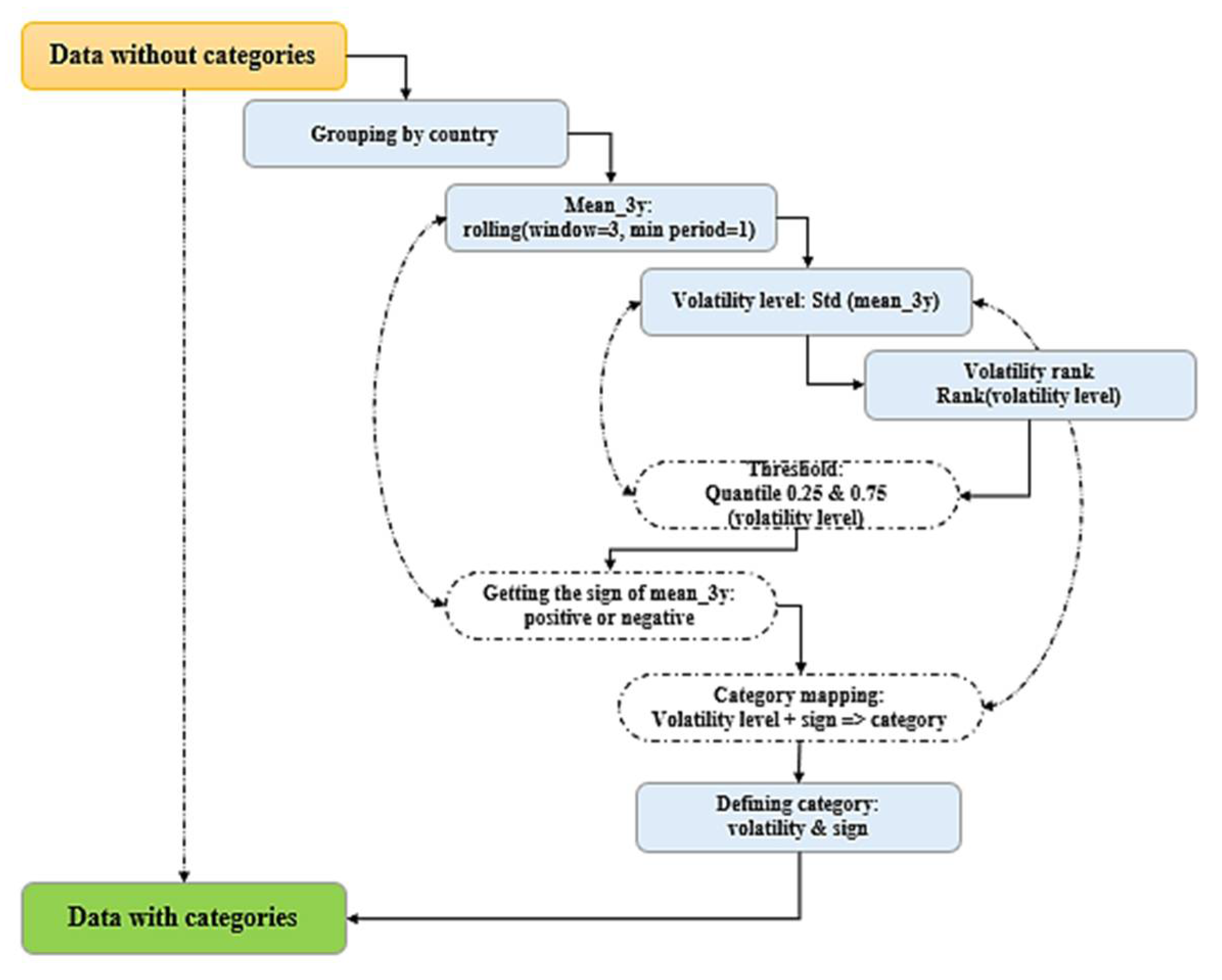
Figure 3.
Research design.
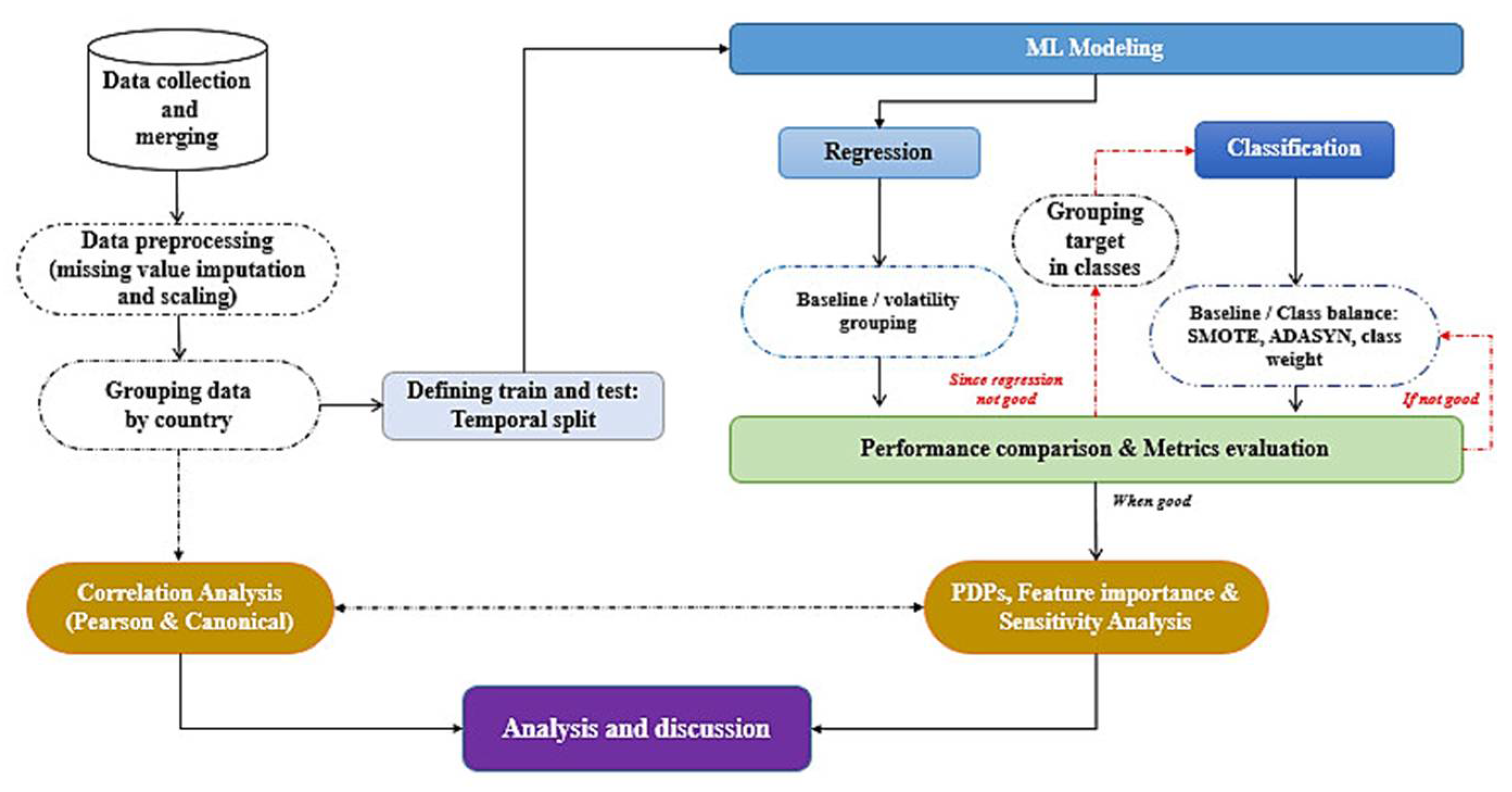
Figure 7.
Classes in the dataset.
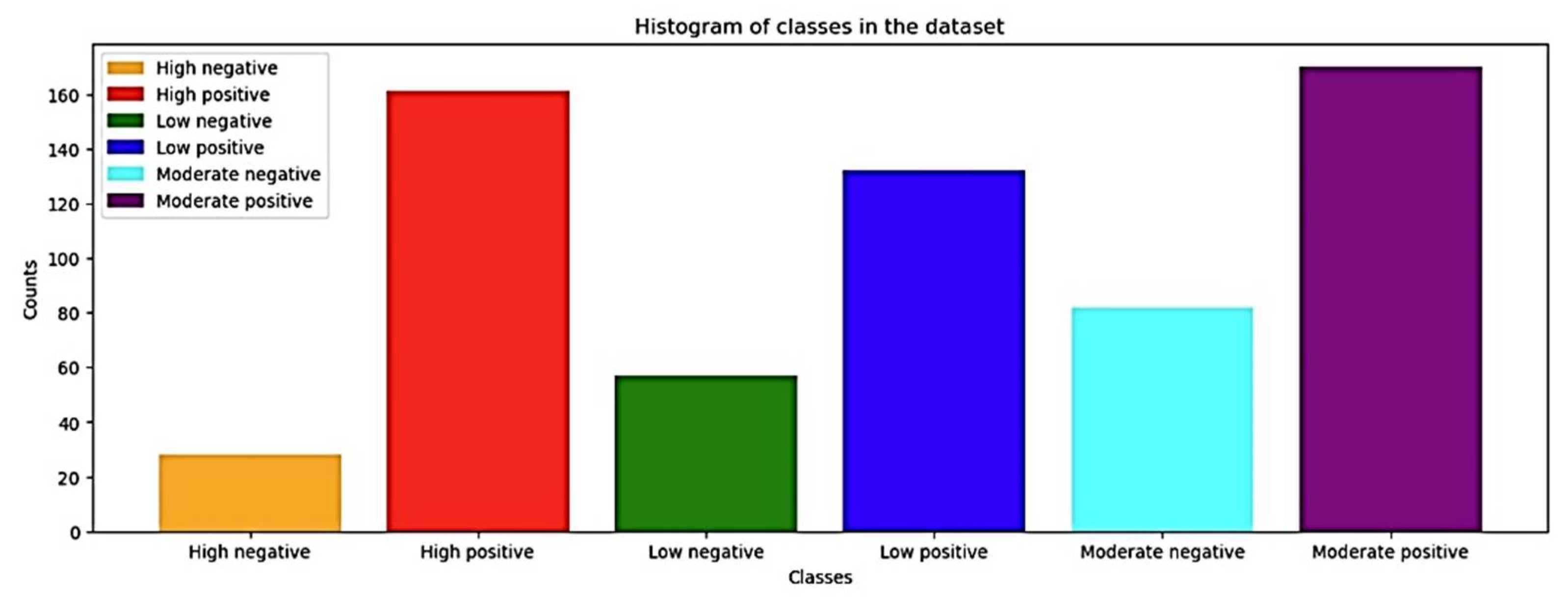
Figure 8.
Temporal dynamics of the target by country.
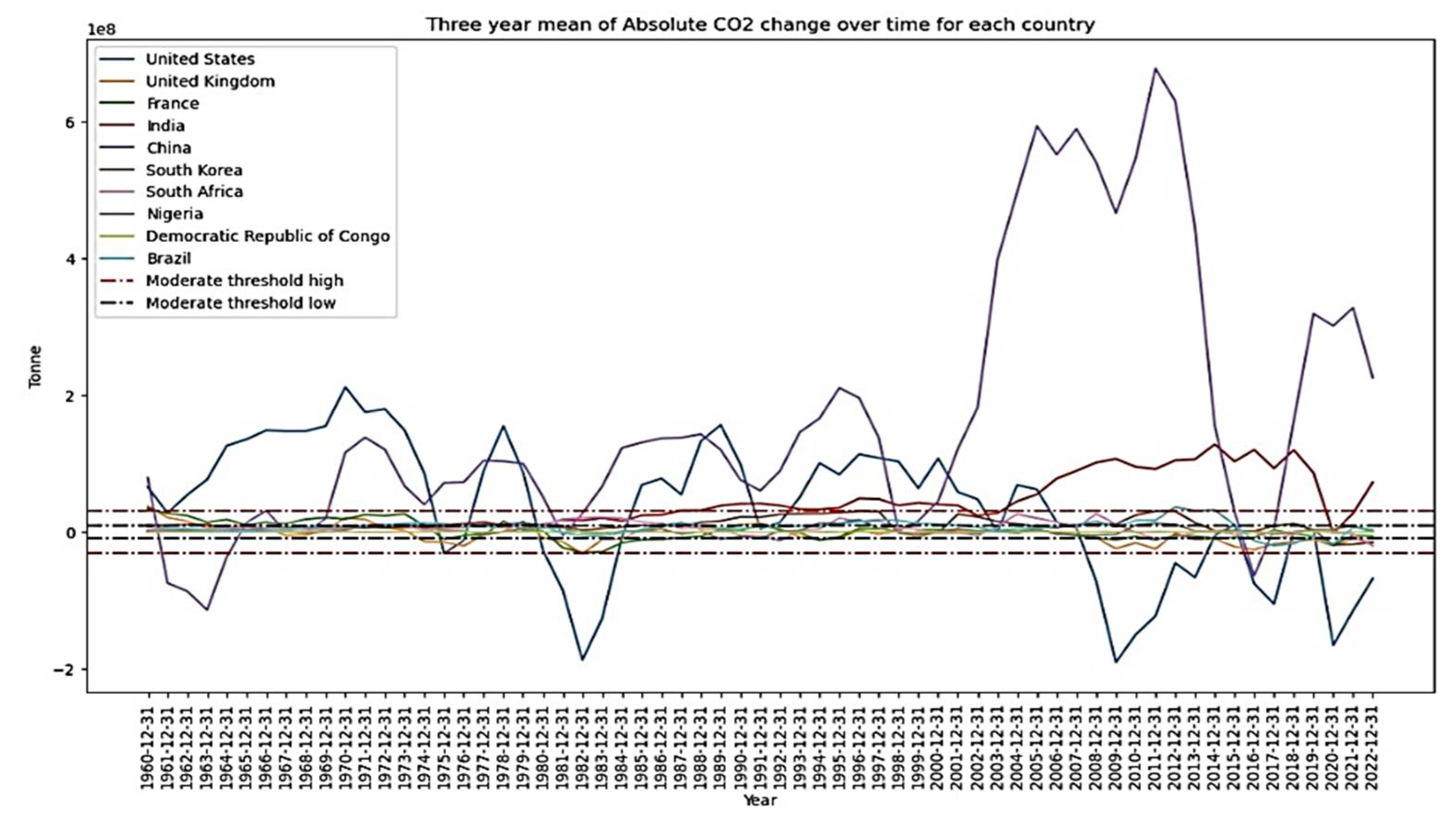
Figure 9.
Dynamics of class overtime.
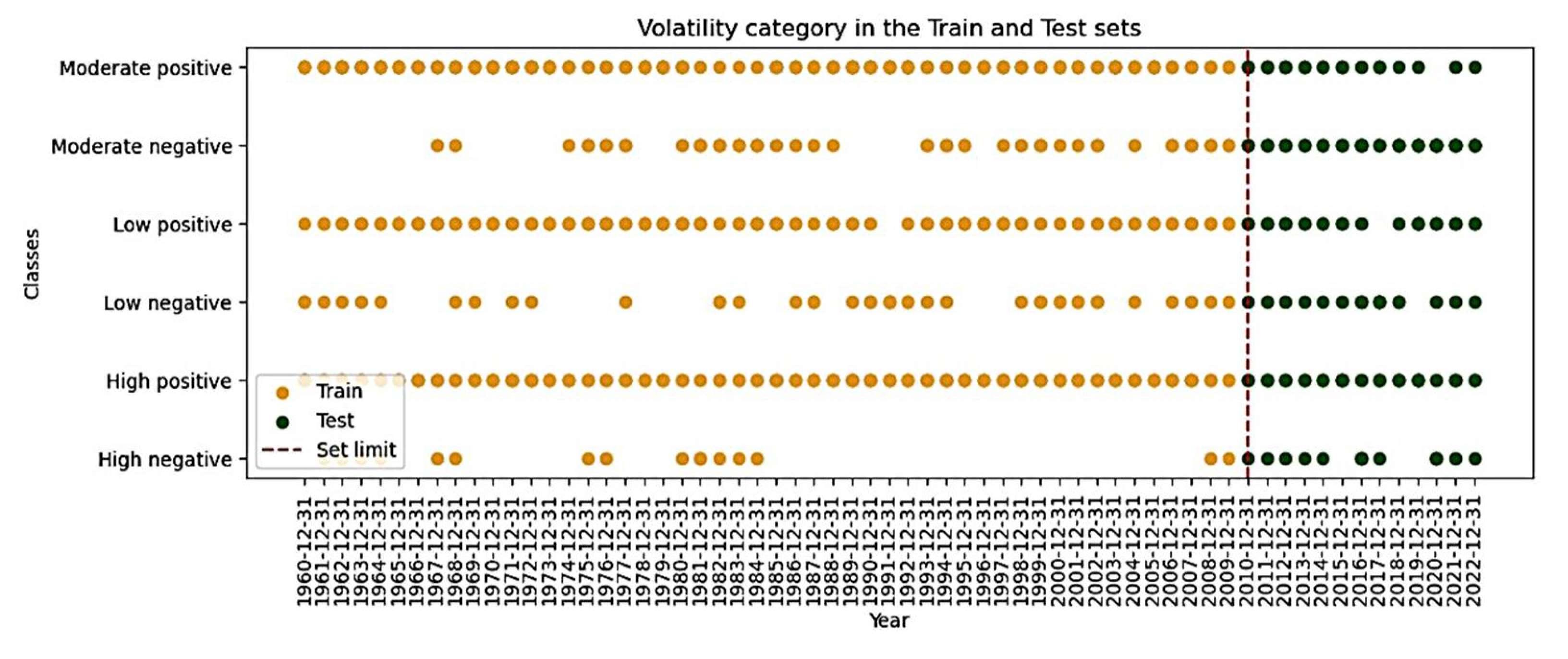
Figure 10.
Importance of features in the decision tree model .
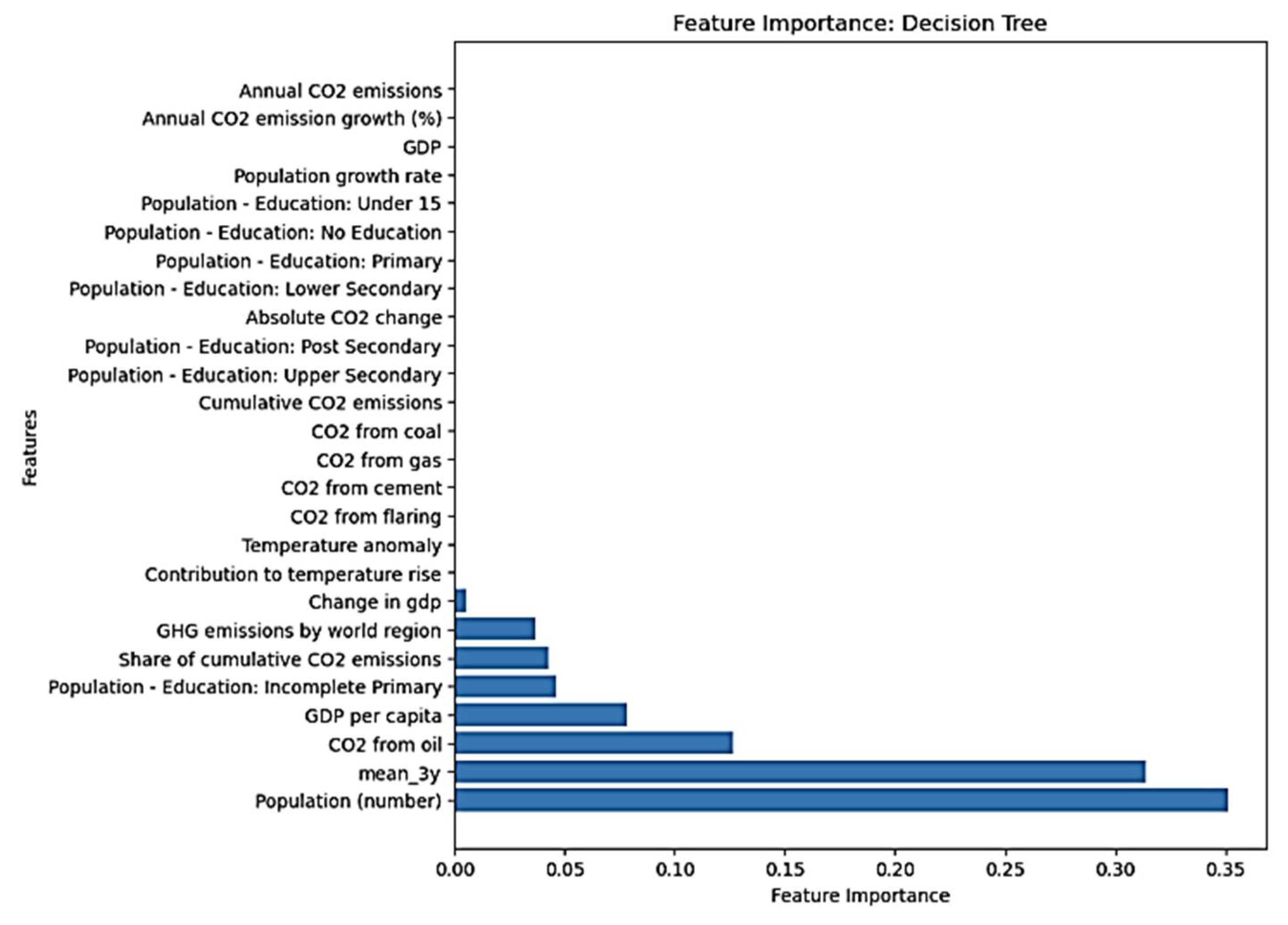
Figure 12.
Sensitivity analysis result.
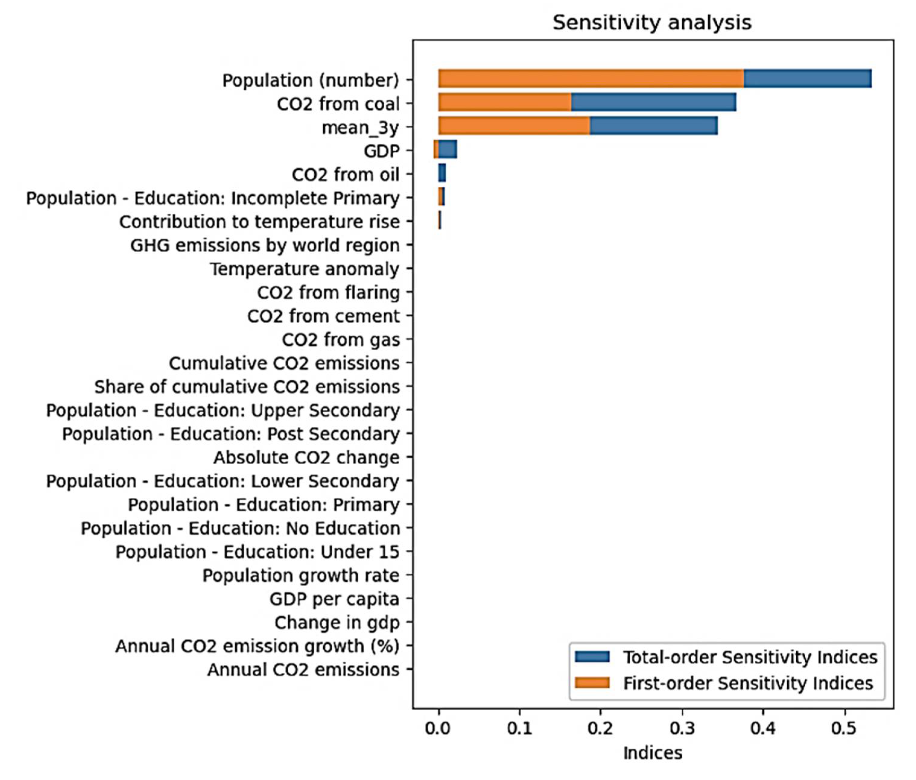
Figure 13.
Correlation table.
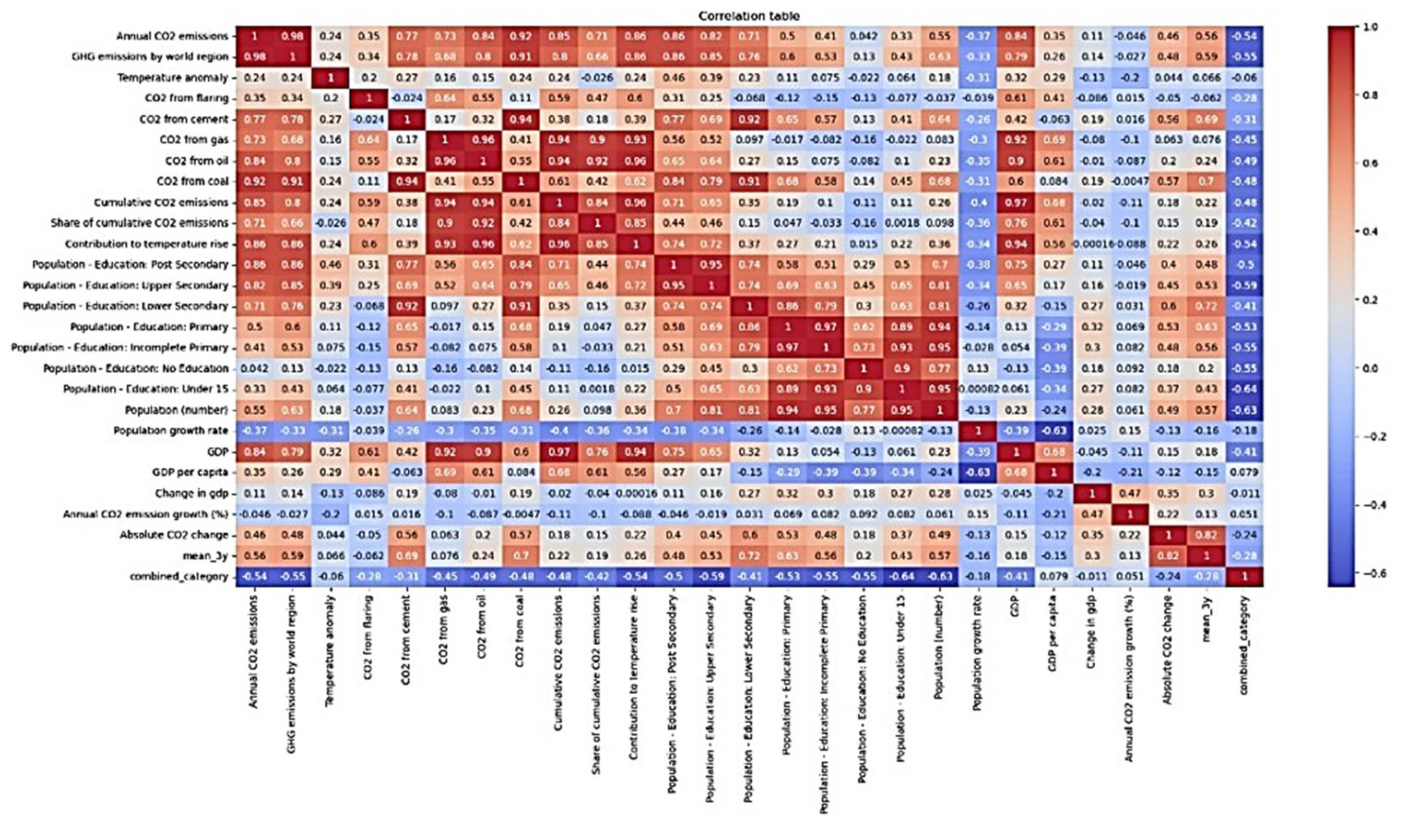
Table 1.
Range of values by classes.
| Category Names | Min Values | Max Values | Range | Countries |
|---|---|---|---|---|
| High positive | 3.244667e+03 | 6.769703e+08 | 676967055.333 | United states, China, India |
| High negative | -1.906534e+08 | -1.370680e+05 | 190516332 | |
| Moderate positive | 4.88107e+05 | 3.741389e+07 | 36925079.3 | United Kingdom, France, South Korea, Brazil, India |
| Moderate negative | -3.209079e+07 | -4.587947e+05 | 31631995.3 | |
| Low positive | 2.683000e+03 | 2.632321e+07 | 26320527 | South Africa, Nigeria, Democratic Republic of Congo |
| Low negative | -2.045842e+07 | -8.609333e+03 | 20449810.667 |
Table 5.
Summary of Classifier’s performance.
| Model | MCC | AUC | Precision | Recall | F1 score | Mean CV |
|---|---|---|---|---|---|---|
| Logreg | 0.67 | 0.73 | 0.76 | 0.73 | 0.68 | 0.74 |
| DT | 0.95 | 0.96 | 0.96 | 0.96 | 0.96 | 0.93 |
| RF | 0.87 | 0.89 | 0.91 | 0.89 | 0.89 | 0.86 |
| XGB | 0.83 | 0.85 | 0.89 | 0.85 | 0.84 | 0.91 |
| GB | 0.84 | 0.86 | 0.89 | 0.86 | 0.85 | 0.85 |
| SVC | 0.58 | 0.64 | 0.70 | 0.64 | 0.58 | 0.73 |
| MLP | 0.60 | 0.66 | 0.74 | 0.66 | 0.64 | 0.75 |
| GNB | 0.50 | 0.58 | 0.66 | 0.58 | 0.55 | 0.75 |
Table 4.
Summary of PDPs analysis.
| Class | Increase | Decrease |
| High negative | Population number | 3 years average |
| High positive | co2 from coal Population number 3 years average |
--- |
| Low negative | --- | Population number Gdp 3 years average |
| Low positive | 3 years average |
co2 from oil Population education: Incomplete Primary Population number Change in gdp |
| Moderate negative | GDP | Population number 3 years average |
| Moderate positive | co2 from oil Population education: Incomplete Primary Change in gdp 3 years average |
Co2 from coal Population number |
Disclaimer/Publisher’s Note: The statements, opinions and data contained in all publications are solely those of the individual author(s) and contributor(s) and not of MDPI and/or the editor(s). MDPI and/or the editor(s) disclaim responsibility for any injury to people or property resulting from any ideas, methods, instructions or products referred to in the content. |
© 2024 by the authors. Licensee MDPI, Basel, Switzerland. This article is an open access article distributed under the terms and conditions of the Creative Commons Attribution (CC BY) license (http://creativecommons.org/licenses/by/4.0/).
Copyright: This open access article is published under a Creative Commons CC BY 4.0 license, which permit the free download, distribution, and reuse, provided that the author and preprint are cited in any reuse.


