
Submitted:
18 July 2024
Posted:
19 July 2024
You are already at the latest version
Abstract
The environmental Kuznets curve (EKC) hypothesis posits an inverted U-shaped relationship between economic growth and environmental degradation. However, there is no consensus regarding the EKC hypothesis among countries and regions of different income groups. In this study, we analyze the EKC hypothesis for 158 countries and 44 regions from 1990 to 2020, categorizing them into different income groups based on the World Bank's income classification (low, lower-middle, upper-middle, and high-income countries). Our findings reveal mixed patterns in the EKC across different income levels, highlighting the heterogeneous relationship between economic growth and carbon emissions and showing differentiated patterns among different income levels. While a rise in income for high-income countries should be reflected in a shift toward fewer carbon emissions, for lower-income countries, growth is still associated with rising emissions. This underscores the urgent need for policy interventions that decouple economic development from environmental degradation. A balanced approach to economic growth, which prioritizes carbon neutrality across all stages of development, by tailoring environmental and economic strategies to address CO2 emissions effectively, should be adopted, recognizing the different developmental stages and income levels of countries and regions.
Keywords:
Environmental Kuznets curve
; CO2 emissions
; Economic growth
; Cross-correlation analysis
; Income levels
; Sustainable development
1. Introduction
For human survival and development, the Earth's climate must be suitable and stable [1,2]. However, according to the Berkeley Earth press release [3], 2023 was the warmest year, with global surface temperatures having accelerated by ~1.5 °C since the pre-industrial period. Human activities and anthropogenic greenhouse gas emissions have been “unequivocally” identified as the main causes of global warming [4]. Considering the identified causality, one issue requires academic and governmental attention: how to change the existing paradigm of development to bring into line with the principles of climate mitigation [5,6,7,8,9].
In the environmental economics literature, the environmental Kuznets curve (EKC) is widely discussed. The EKC is a re-interpretation, from the economics field, of the nonlinear relationship between per capita income and income inequality, proposed by Kuznets [10]. In the 1990s, Grossman and Krueger [11] proposed the EKC concept to describe the inverted U-shaped relationship between economic growth and environmental degradation. The EKC links economic development with environmental quality and posits that at the early stages of economic development, due to the higher priority given to income over environment, both economic growth and environmental pollution would increase. However, after a certain point of economic development, as a greater proportion of the population is willing to pay for a clean environment, and due to more effective environmental policies, this scenario would be reverted, and pollution would start declining. This means that in the early stages of development, there exists a positive relationship between environmental degradation and per capita income (a positive slope), but after a certain level of growth, pollution decreases with an increase in per capita income, i.e., a negative slope [12,13,14].
Given the above, it was expected that most developed countries would display an inverted U-shaped relationship between economic growth and environmental degradation. However, several recent studies point out that some developed countries are ecologically deficient (see, for example, [15,16]); there are also other countries (such as Germany, the Netherlands and Austria), which are once again turning to coal for electricity and heating, as they struggle with a European energy crisis triggered by the Russia–Ukraine conflict beginning in 2022 [17,18]. Furthermore, it is important to test the relationship between environmental quality and economic growth as it allows policymakers to judge the response by the environment to economic growth; this is crucial since the objective function of any economy is to maximize economic growth. Moreover, it is crucial to consider the targets for global carbon neutrality and net zero carbon emissions by 2050, which are central to international climate policies. Many high-income countries have committed to achieving net zero emissions by mid-century, implying significant changes in energy production and consumption. These targets underscore the necessity for sustainable development where economic growth is decoupled from carbon emissions. Integrating these targets into EKC analyses can provide relevant insights into the alignment of economic and environmental policies and identify gaps and opportunities for improvement in climate mitigation strategies. Thus, we revisit the EKC by considering recent data (from 1990–2020) and a broad set of countries, grouped by their income levels, to identify for which exists (or does not exist) evidence of an inverted U-shaped relationship between income level (measured by the GDP per capita) and environmental degradation [measured by carbon dioxide (CO2) emissions per capita]. The study also aims to identify if there are differences in how GDP and CO2 are related in different groups of countries. To perform this assessment, providing an empirical contribution, we test the EKC hypothesis by applying the cross-correlation coefficient (CCC) approach of Narayan et al. [19].
Our findings reveal that low-income countries display the highest percentage of countries aligned with the EKC hypothesis, while high-income countries display the lowest. However, there are countries whose behavior is partially aligned with the EKC hypothesis, i.e., countries for whom it is expected that CO2 emissions will reduce in the future with increased GDP. In this case, high-income countries display the highest percentage of alignment, while none of the lower-income countries reveals a trend of CO2 reduction in the future with an increase in GDP. Across the world, there are significant variations in the alignment with the EKC hypothesis. Generally, Europe and Asia are the world regions whose behavior best fits the EKC hypothesis. Our results also reveal that 11.36% of the world regions are on a carbon neutrality path where economic growth is decoupled from carbon emissions.
This article is organized as follows: Section 1, which presents the motivation for this study and the main results; Section 2, which provides a brief literature review of the studies related to the EKC hypothesis; Section 3, which provides an overview of the analyzed data and the applied methods; Section 4, which discusses the results, and Section 5, which offers some concluding remarks.
2. Brief Literature Review
Climate change and its consequences for the global economy have been discussed in the economic literature since the 1980s [20]. In recent years, one of the major concerns of nations has become global warming, particularly its adverse effects on the Earth, and implicitly, on the quality of life. The start of the Industrial Revolution contributed to significant changes at the global level (both economically and socially) with subsequent effects on the environment. Thus, reducing emissions of greenhouse gases (GHG), such as CO2, methane (CH4), nitrous oxide (N2O), and a set of fluorinated gases [hydrofluorocarbons (HFCs), perfluorocarbons (PFCs), sulfur hexafluoride (SF6), and nitrogen trifluoride (NF3)] is the key to mitigating climate change.
The EKC, which emerged in the early 1990s [11], is one hypothesis linking economy and environmental quality. Grossman and Krueger [21] identified evidence of a nonlinear relationship between income and environmental quality and proposed an inverted U-shaped relationship between both variables. According to their theory, the GDP per capita initially leads to greater environmental deterioration at low-income levels, but other factors may eventually cause an improvement in environmental quality with further economic development.
The EKC theory, which suggests an inverted U-shaped relationship between environmental degradation and income, has been the subject of much debate (see, for example, [22,23,24,25,26] for extensive and systematic literature reviews in this regard, which are not covered by this research since we do not aim to review or cite all the rapidly growing number of studies).
For example, Ekins [27] examined the evidence for an EKC relationship between environmental quality and income. They found that important indicators show a monotonically increasing (rather than inverted-U) relationship between environmental quality and income. Furthermore, they concluded that the income-environment relationship is still very problematic from the environmental sustainability perspective and determined that environmental policies will be required to make income growth compatible with sustainable development. Cole [22] provided a comprehensive analysis of the relationship between economic growth and environmental degradation, reviewing historical debates and examining recent statistical studies on the topic. The authors found that the EKC studies suggest that some environmental indicators appear to improve with growth, while others deteriorate, indicating a need to interpret EKCs carefully.
The EKC hypothesis suggests that economic growth improves environmental quality [23], but research findings are mixed. More studies are needed to understand the relationship between economic growth and sustainability. Policy measures are necessary to promote sustainability, and economic models should incorporate better the physical and ecological aspects of economic activity and the interaction between the economy and the environment.
Following the same line of thinking, Ekis [27] and Aslanidis [28] also questioned the existence of a clear EKC and provided a critical review of the literature on the EKC for carbon emissions. The author found no clear-cut evidence supporting or rejecting the existence of the EKC for carbon emissions despite using more sophisticated econometric techniques. The assumption of homogeneous income effects across countries is rejected, with the EKC holding true only for some developed countries. Carbon emissions and GDP per capita are integrated variables, although not always co-integrated, which casts doubt on the validity of the EKC [14].
Mbatu and Otiso [29] examined the environmental, ecological, and sociopolitical impacts of Chinese economic expansionism in Africa, particularly in the Cameroonian forest sector, and concluded that this engagement is detrimental to African peoples and their environment. They argue that the EKC hypothesis can be misleading or dangerous, as it requires a very high threshold of economic development before environmental quality begins to improve. Chen et al. [30] argue that the EKC pattern may not be valid for situations of more damaging pollution, given human-bounded rationality and societal uncertainties. Conversely, Purcel [24], in a literature review of the EKC hypothesis found that recent empirical studies indicate a consensus on the pollution-growth nexus and EKC validity in developing and transition economies. Several other studies also found a long-term relationship between pollution and growth, supporting the EKC hypothesis.
Although the EKC knowledge domain has developed substantially since its inception, no consensus exists on the existence, shape, and turning points of the EKC among researchers [26]. While several studies validated the existence of the EKC while dealing with a wide sample of economies, other multi-country studies failed to validate this theory, and some others found mixed evidence (see, for example, [31], for an extensive state-of-the-art review). Moreover, only a few studies explore the cross-correlation between per capita GDP and environmental degradation indicators over the lags and leads, i.e., past and future, by reinforcing the concept of the ECK hypothesis. However, there are several exceptions cited in literature [19,32,33,34,35]. Using the EKC hypothesis, these studies have explored the relationship between economic growth, CO2 emissions, globalization and environmental degradation. Some studies found evidence supporting the EKC hypothesis in countries with different income levels, suggesting that income growth can reduce CO2 emissions and environmental degradation. However, the impact of factors such as financial development and tourism revenues varies depending on the country's income level. Additionally, the role of exports and imports in sustainable development in developing countries was also examined, with exports showing positive effects and imports having negative impacts. Overall, the results provide insights into how different factors influence environmental outcomes in various countries.
Despite the huge number of studies that test the EKC hypothesis by considering panel data analysis, and although some use larger groups of countries, most of them investigate the EKC validity by considering almost exclusively developing and transition economy samples. Alternatively, they use specific groups of countries, justifying revisiting the EKC hypothesis by considering a broad set of countries and world regions, as well as also using more recent data. Furthermore, studies on the relationship between GDP per capita and CO2 emissions, using the cross-correlation approach, and considering the lag and lead relationship, still need to be more extensive, leaving a gap in research and highlighting the need for more. This approach represents an important inquiry in this research stream, to determine how the GDP per capita might lead to a reduction in CO2 emissions.
3. Data and Methods
3.1. Data
To test the EKC hypothesis, data on GDP per capita (current US$) and CO2 emissions (metric tons per capita) were retrieved from the World Bank (https://data.worldbank.org/). Carbon dioxide emissions are a leading indicator of environmental pollution and are used in several studies that test the EKC hypothesis (see, for example, [24] for a survey of studies that use this indicator in this regard). The data covers 193 countries and 46 world regions.
To analyze a similar period for all the countries and regions, and due to data availability for both variables selected (GDP and CO2 emissions), the analysis covers 158 countries. As for the world regions South Asia and South Asia (IDA and IBRD), and for Sub-Saharan Africa and Sub-Saharan Africa (IDA and& IBRD countries), the values of GDP per capita and CO2 emissions are the same, the world regions South Asia (IDA & IBRD) and Sub-Saharan Africa (IDA & IBRD countries) were not considered. The IDA countries include those countries that receive concessional loans (low or zero interest) from the International Development Association (IDA). On the other hand, the IBRD countries include both middle-income and creditworthy low-income countries that receive loans from the International Bank for Reconstruction and Development (IBRD) for development projects. Thus, 44 world regions were considered. The data ranges from 1990 (the first year for which there are available data on CO2 emissions) to 2020 (the last year with data on CO2 emissions).
To compare the results, the countries were then grouped into categories based on their income level (which evolves over time). For this classification, the last year of available data (2020) was considered, as detailed in Table 1. These categories follow the World Bank Group assignments, which are widely used and recognized in economic literature. Specifically, the countries were grouped into low, lower-middle, upper-middle, and high-income levels. This classification is based on the Gross National Income (GNI) per capita (in US$, converted from the local currency using the Atlas method). This classification provides a standardized and reliable framework for comparing economic and environmental data across different income levels.
As countries are at different stages of development, their incomes per capita are different. Thus, and as hypothesized by the EKC hypothesis, this has direct implications for the magnitude of carbon emissions, meaning it is relevant to their classification by income level.
3.2. Methods
The EKC hypothesis is tested using the cross-correlation coefficient (CCC) proposed by Narayan et al. [19], which states that a reduction in CO2 emissions with an increase in income over time will be observed if: (i) there is a negative cross-correlation between the current level of income and the future level of CO2 emissions, and (ii) there is a positive cross-correlation between the current level of income and the past level of CO2 emissions. This cross-correlation coefficient is estimated according to equation (1):
where and are, respectively the mean GDP and CO2 emissions per capita, and t ranges from 1 to 31 (since we have yearly observations for the 31 years from 1990 to 2020).
To avoid spurious correlations between the analyzed variables, both time series are detrended with the Hodrick–Prescott (HP) filter, which uses a mathematical equation that minimizes the sum of the squared differences between the original time series (cyclical component) and the trend component (which represents the long-term underlying growth or decline in the series), subject to a constraint on the smoothness of the trend component. This filter is, among the data-smoothing techniques, one of the most commonly used in the literature [36,37], and uses a lambda (λ) parameter to control the trade-off between smoothing the trend and preserving the data fluctuations.
Considering the annual frequency of the data used, the λ parameter was set as λ=100. After detrending the series, the CCC was estimated for the lags , which are sufficient to gauge the behavior of CO2 emissions in response to changes in income [19]. Where we obtain the CCC between and lead or future values of CO2 where we obtain the CCC between and the one-period lead or future value of CO2 . Where the CCC between and is obtained which is the contemporaneous correlation between both variables. On the other hand, where , we obtain the CCC between and the period lag values of CO2.
The EKC hypothesis is considered correct if there exists: (i) a negative cross-correlation between the current level of GDP and future levels (leads) of CO2 emissions (, and (ii) a positive cross-correlation between the current level of GDP and past levels (lags) of CO2 emissions (; CO2 emissions will decline with the progression of GDP over time after a certain point.
4. Results and Discussion
4.1. Preliminary Results
Table 2, Table 3, Table 4, Table 5 and Table 6 present some descriptive statistics, namely the mean and standard deviation (Std.Dev.) for both time series. Table 2, Table 3, Table 4 and Table 5 report the results for the countries (which are grouped according to the categories in Table 1), and Table 6 reports the results for the world regions. The penultimate column of each table shows the values of the unconditional correlation between GDP and CO2 emissions per capita. The null hypothesis of unconditional correlation equal to zero was tested (with a t-test using the t-statistics), and the results are displayed in the last column.
As was expected, high-income countries report higher mean GDP (and standard deviation) values, and generally higher mean CO2 emissions. However, it is curious to observe that the Principality of Monaco reports the highest mean GDP value but does not report one of the highest values of mean CO2 emissions. Monaco’s highest mean value of GDP per capita can be explained by its robust financial sector, luxury tourism, and the presence of wealthy residents. Unlike countries with high industrial output, Monaco's economy does not rely on heavy manufacturing or large-scale industrial activities that typically result in significant CO2 emissions. Thus, despite its high economic wealth, Monaco has a low carbon footprint, which may reflect Monaco’s implementation of stringent environmental regulations and sustainable practices. This combination of a service-oriented economy and proactive environmental policies could explain why Monaco enjoys a high GDP per capita without correspondingly high CO2 emissions.
On the other hand, Qatar is the country that reports the highest mean value of CO2 emissions, which can be explained by the extensive oil and gas industry, which is a major contributor to the country's economy. Despite the significant revenues from hydrocarbons, Qatar's wealth distribution, population size and economic structure result in a lower GDP per capita compared to other countries with diversified and technologically advanced economies. Qatar's economic model, which is heavily reliant on fossil fuels, could explain its high CO2 emissions but without a corresponding high GDP per capita.
The countries with the highest levels of CO2 emissions are Bahrain, Kuwait, Qatar and the United Arab Emirates, all of which are countries with large reserves of oil and natural gas (the exploitation of these natural resources being fundamental pillars of their economies) and economies that are heavily dependent on the production and export of hydrocarbons, which can explain their higher values of mean CO2 emissions.
Considering the values of estimated unconditional correlation (between the mean GDP per capita and the mean CO2 emissions per capita), the relationship between GDP and CO2 emissions per capita varies significantly between the different groups of countries, according to their stage of economic development. Except for the high-income countries, most of the correlations are positive and statistically significant, meaning that, on average, incomes have led to increased emissions over the 1990–2020 period; this is in line, for example, with the findings of Narayan et al. [19].
For the high-income countries, 24 unconditional correlations (of the 47 possible) are negative and statistically significant, which could mean these countries passed the inflection point of the EKC. These results seem to be not only in agreement with the EKC hypothesis but also with the energetic transition theory, which suggests that as countries develop, they pass from traditional energy sources to renewable and clean energy sources. From high-income countries to low-income countries (as the income levels decline), the percentage of positive and statistically significant correlations increases. This preliminary evidence seems to agree with the EKC hypothesis, i.e., countries of high-income levels seem to have reached a point where their economic growth is not strongly associated with an increase in CO2 emissions.
The evidence found for the upper-middle and lower middle-income countries could be a sign that these countries are still in the ascending phase of the EKC, where economic growth results in higher levels of CO2 emissions.
Concerning low-income countries, although this category has the smallest number of countries, 77.78% of these countries display positive and statistically significant unconditional correlations, suggesting that even in the early stages of development, there exists a clear relationship between economic growth and CO2 emissions.
Considering the world regions, North America, post-demographic dividend regions (mostly high-income countries where fertility has transitioned below replacement levels), and high-income regions, are the ones that report the highest level of mean GDP per capita and simultaneously the highest mean values of CO2 emissions. The Euro area follows these regions in terms of mean GDP per capita but not in terms of mean CO2 emissions, which the OECD members follow. This could mean that countries outside the Euro area are the major ones responsible for CO2 emissions among the OECD members (as only 19 of the 38 OECD members are from the Euro area). This could also be a sign that the Euro area could have implemented more effective policies and technologies in terms of the reduction of CO2 emissions than other members of the OECD. Thus, the Euro area could be viewed as an example of how high levels of development can coexist with lower levels of emissions through strict environmental policies. Regarding the OECD countries, our results do not seem to agree with the EKC hypothesis, which contradicts the findings of Galeotti et al. [38], who found evidence for the EKC. This could be a sign that OECD countries may need to address the global nature of environmental issues.
The relationship between GDP and CO2 emissions per capita also varies between the different world regions, with most of the correlations being positive and statistically significant, meaning that, on average, incomes have led to increased emissions over the 1990–2020 period. The world, as a whole, displays a positive and statistically significant correlation between the analyzed variables, meaning that global economic growth and CO2 emissions are still strongly associated, which could mean that the world as a whole is still at an early or intermediate stage on the EKC.
Globally, 40 out of the 158 countries (25.3%) and 11 of the 44 world regions (25%) display a negative and statistically significant unconditional correlation between GDP and CO2 emissions per capita. This percentage is higher than the one found by Narayan et al. [19], which, considering the period 1960–2008, found 20 countries (of 181 analyzed) with this pattern. These results indicate that, as GDP per capita increases, CO2 emissions decrease, reflecting a significant change in the traditional relationship between economic growth and CO2 emissions, which could mean that economic growth is no longer necessarily associated with higher CO2 emissions in many countries. At the same time, and considering the perspective of the EKC, this could mean that more countries have reached the inflection point or are in the process of reaching it. However, this transition is not yet universal, which is confirmed by the different results for the world regions.
4.2. Cross-Correlation Coefficient Analysis
The correlations obtained in the previous sub-section are static and do not allow us any insight into how these relationships will behave in the future. Thus, to get some insights in this respect and evaluate how GDP per capita is negatively or positively correlated with CO2 emissions over the past (lags), and in the future (leads), the CCC proposed by Narayan et al. [19] was estimated, and the results are displayed in Table 7, Table 8, Table 9 and Table 10 for countries (which are grouped according to the categories in Table 1) and in Table 11 for world regions.
The third and fifth columns of each table report the sum of the cross-correlation coefficients over the past 20 lags and the future 20 leads of CO2 emissions, respectively. The fourth and sixth columns report the mean values of the same lags and leads, respectively. If past/future values of CO2 emissions per capita, i.e., lags/leads, are positively/negatively correlated with the current values of GDP per capita, there is evidence of an inverted U-shaped relationship (identified with an “X” in the seventh column of Table 7, Table 8, Table 9, Table 10 and Table 11). This means that the CO2 emissions increased with GDP in the past, but will decline in the future, supporting the EKC hypothesis. However, in addition to this scenario, another three can be observed: (i) negative cross-correlation between both past and future values of CO2 emissions (lags and leads) and the current level of GDP per capita (identified with an “X” in the eighth column of Table 7, Table 8, Table 9, Table 10 and Table 11), meaning in this case, increasing GDP per capita has led in the past, and could lead in the future, to a reduction in carbon emissions, which partially supports the EKC hypothesis; (ii) past/future values of CO2 emissions per capita, i.e., lags/leads, could be negatively/positively correlated with the current values of GDP per capita, meaning that, although in the past an increase in the GDP level led to a reduction of CO2 emissions per capita, in the future it will not happen (identified with an “X” in the ninth column of Table 7, Table 8, Table 9, Table 10 and Table 11); (iii) positive cross-correlation between both past and future values of CO2 emissions (lags and leads) and the current level of GDP per capita, meaning in this case, increasing GDP per capita has led in the past, and will probably lead in the future, to an increase in carbon emissions (identified with an “X” in the tenth column of Table 7, Table 8, Table 9, Table 10 and Table 11).
To verify whether our results are consistent, we begin our analysis by verifying whether the sign of the sum of the CCC for the lags and leads and their averages are similar, i.e., whether they are both (sum and average) negative or positive. As displayed in Table 7, Table 8, Table 9, Table 10 and Table 11, they are. Thus, we can consider as valid the values of the averages of the CCC in our analysis.
Considering the results of the average CCC (that can soften outliers and provide a clearer view of the general pattern), displayed in Table 7, for the 47 countries categorized as high-income countries, only three (namely, The Bahamas, Monaco, and Poland) show signs of an inverted U-shaped relationship between the current levels of GDP per capita and past and future values of CO2 emissions. On the other hand, Czechia, Germany, Hong Kong, Luxembourg, Singapore, the Slovak Republic, Sweden, Switzerland, and the United Arab Emirates (a total of nine countries), reveal negative mean values of the CCC over the lags and leads, which may be a sign that for these countries the CO2 decreased in the past and will continue to decrease in the future, with the increase in GDP per capita. These results partially agree with the EKC hypothesis and corroborate the results of Narayan et al. [19] in the cases of Czechia, Luxembourg, the Slovak Republic, Sweden and Switzerland. For the majority of high-income countries (26 countries), we find a negative cross-correlation for the lags and a positive for the leads, which could mean that although, in the past, an increase in GDP level led to a reduction of CO2 emissions per capita, it will not happen in the future. The remaining countries of this panel (precisely, nine countries) display positive cross-correlation for the lags and leads, meaning that increasing GDP per capita has led in the past, and will probably lead in the future, to an increase in carbon emissions.
Considering the 44 upper middle-income countries, the results suggest that 10 countries (namely, Armenia, Azerbaijan, Botswana, Colombia, Iraq, Kazakhstan, Romania, the Russian Federation and Suriname) agree with the EKC hypothesis, although Bulgaria is only in partial agreement. For the remaining countries in this panel, 17 reveal negative/positive cross-correlations for the lags/leads and 16 positive cross-correlations for the lags and leads.
For the lower middle-income countries, 12 (namely, Algeria, Belize, Bolivia, Cameron, the Congo Republic, Eswatini, the Kyrgyz Republic, Mongolia, Tanzania, Vanuatu, Zambia and Zimbabwe) show evidence of an inverted U-shaped relationship, and three (Nigeria, Ukraine and Uzbekistan) are only in partial agreement with the EKC hypothesis, displaying negative average CCC for the leads. For the remaining countries (34), the results do not provide any support for the EKC hypothesis.
For the panel of 18 lower-income countries, four (namely, Burundi, the Central African Republic, Guinea-Bissau, and Malawi) show an inverted U-shaped relationship. For the remaining 14 countries, two (Togo and the Yemen Republic) reveal negative/positive cross-correlations for the lags/leads and 12 positive cross-correlations for the lags/leads.
If we compare our results with those of Shahbaz et al. [32], who explored the nexus between globalization and energy demand for 86 high, middle, and low-income countries over the period 1970–2015, we can highlight that: (i) some countries have changed, in relation to the income level criteria, their category/classification; (ii) several countries of different income levels (but mostly from high-income levels) have maintained or improved the relationship between the mean GDP per capita and the mean CO2 emissions for the lags, but have displayed a similar pattern for the leads. However, there are four countries, namely Denmark, the United States, Gabon and the Philippines, which, although revealing a similar pattern for the lags, display a positive (sum and average) CCC for the leads [while in the study of Shahbaz et al. [32] they displayed a negative CCC (sum and average), indicating an undesirable inversion on their pathway to sustainable development; (iii) on the other hand, Botswana, Algeria, Bolivia and the Congo Republic, although revealing a similar pattern for the lags, display a negative (sum and average) CCC for the leads (while in the study of Shahbaz et al. [32] they displayed a positive CCC (sum and average)), also indicating an inversion on their pathway to sustainable development. However, for these countries, it is a desirable one, since a reduction in CO2 emissions is expected with increasing GDP; (iv) for Albania, Ghana and Sudan, increasing GDP has led in the past, and will lead in the future, to rising CO2 emissions, entirely contradicting the findings of Shahbaz et al. [32]; (v) on the other hand, for Sweden and Nigeria, increasing GDP has led in the past, and will lead in the future, to decreasing CO2 emissions, also entirely contradicting the findings of Shahbaz et al. [32].
Considering the results of the average CCC displayed in Table 11, for the 44 regions, only three (namely, Europe & Central Asia (excluding high-income), Europe & Central Asia (IDA & IBRD countries) and Pre-demographic dividend) show signs of an inverted U-shaped relationship between the current levels of GDP per capita and past and future values of CO2 emissions. This evidence suggests that these regions are managing to balance economic growth with effective environmental policies. On the other hand, Central Europe and the Baltics, Europe & Central Asia, fragile and conflict-affected situations, IDA blends, and low-income regions, reveal negative mean values of the CCC over the lags and leads, partially supporting the EKC hypothesis. For fragile and low-income regions, it may be a positive sign that economic growth is not being achieved at the expense of increasing carbon emissions, but these results may also reflect economic challenges that limit growth. For 13 regions, the results reveal negative cross-correlation for the lags and positive ones for the leads, which could mean that although in the past an increase in GDP level has led to a reduction in CO2 emissions per capita, in the future, this will not happen. These results may indicate that these regions may face the risk of reversing the environmental gains they have achieved in the past, which may be due to a possible lack of continuity in environmental policies or new economic challenges. Thus, for these regions, there is an urgent need to implement or reinforce environmental policies that ensure that future economic growth does not increase CO2 emissions. Finally, the majority of regions (23) display positive cross-correlation for the lags and leads, meaning that increasing GDP per capita has led in the past, and probably will lead in the future, to an increase in carbon emissions. In these regions, the growth of per capita GDP has historically led, and will probably continue to lead, to a rise in CO2 emissions, which may indicate that these economies are at an early stage of the EKC. It is, therefore, essential that these regions adopt strict environmental policies and promote clean technologies to reverse this trend.
Table 12 summarizes all the above results for a brief and easier analysis. The first column ((+)/(-)) identifies the number and percentage of countries and regions that, considering the average CCC for the 20 lags and 20 leads, reveal a pattern in agreement with the EKC hypothesis. The second column identifies the number and percentage of countries and regions that reveal a pattern in partial agreement with the EKC hypothesis. The last two columns show the number and percentage of countries and regions for which it is expected that, in the future, there will be an increase in CO2 emissions with GDP per capita. It is interesting to note that high-income countries are the ones that are in least agreement with the EKC hypothesis. It was expected that these countries, being economically well-established and having the necessary infrastructure and resources to maintain and promote a cleaner environment, would be in greater agreement with the EKC hypothesis, but this is not verified.
Generally, the results suggest that 18.35% of the countries (29 out of 158) and 6.82% of the world regions (three out of 44) support the EKC hypothesis. Comparing our results with the ones of Narayan et al. [19], which found 12% with clear evidence supporting the EKC hypothesis), the percentage of countries in agreement with this hypothesis has increased. Considering the countries/regions that are in partial agreement, i.e., the ones in which it is expected that an increase in the GDP will be accompanied by a reduction in CO2 emissions in the future, our results reveal that only 8.23% of countries, and 11.36% of world regions, seem to be aligned with this pattern. If we compare this result with the one of Narayan et al. [19], which found that 27% of the countries partially agree with the EKC hypothesis, our results are not very encouraging regarding CO2 reductions in the future. According to our results, it is expected that 73.42% of countries and 81.82% of world regions will see an increase in CO2 emissions with an increase in GDP.
For a more accurate analysis of which countries and regions agree with the EKC hypothesis using the CCC proposed by Narayan et al. [19], it is crucial to consider both the average values of the lags and leads as well as the detailed graphical representation of these coefficients over the 20 lags and 20 leads. Although the average values of the lags and leads provide a simplified and aggregated view of the relationship between GDP and CO2 emissions, we must not forget some possible limitations related to this analysis. Using averages can mask significant variations and trends within the individual lag and lead periods. Furthermore, a graphical presentation of the CCC for each of the 20 lags and leads allows a more nuanced and detailed analysis. The graphs will enable us to highlight the specific periods where the relationship changes, providing relevant information about the temporal dynamics that the average values cannot capture. For instance, a graph might show that the correlation is positive for the initial few lags/leads but starts to decline and eventually turns negative as we approach the 20th lag/lead. This transition is critical in understanding how economic activities can influence environmental outcomes over time and supports a more robust interpretation of whether a country/region agrees with the EKC hypothesis. Moreover, graphical analysis can help us identify any anomalies or outliers that could significantly affect the average values. Visualizing the CCC over time can also illustrate the consistency or volatility of the relationship between the analyzed variables, providing context essential for interpreting the results accurately. This dual approach ensures that we capture the full complexity of the relationship between the analyzed variables, allowing more accurate conclusions about agreement of countries/regions with the EKC hypothesis. For these reasons, Figure 1 displays the plots for the countries/regions whose behavior seems to agree with the EKC hypothesis (with reference to the positive sign (+) for the average CCC for the lags, and the negative (-) one for the average CCC for the leads), and Figure 2 displays the graphs for the countries/regions which seem to be in partial agreement with the EKC hypothesis, i.e., the ones that display negative sign (-) for the average CCC for the leads. We plotted the graphs for the 20 lags and leads for all the countries and regions (a total of 202 graphs). However, due to space constraints, it is not possible to present all of them here, but they are all available upon request.
5. Conclusions
Due to concerns about global climate change, the number of studies related to CO2 emissions has increased in recent decades. Although most studies empirically identify a relationship between economic growth and environmental negative indicators in the context of the EKC, the results do not always agree, highlighting the need for deeper analysis.
This study looked at GDP and CO2 emissions per capita from 1990 to 2020 in 158 countries and 44 world regions. Countries were grouped into income levels, with high-income countries showing the lowest alignment with the EKC hypothesis (CO2 reduction with GDP increase), while lower-income countries showed the highest alignment. For high-income countries, there was a higher percentage of countries partially aligned with the EKC hypothesis. It was found that CO2 emissions may be reduced in the future with increased GDP for high-income countries but not for lower-income countries. High-income and upper middle-income countries may not see a reduction in CO2 emissions with GDP increase in the future, indicating a need for reinforcement of environmental policies and investment in green technologies. Upper middle-income countries should transition to more sustainable practices like renewable energy adoption and energy efficiency improvements.
In lower-middle and lower-income countries, a high percentage of nations have shown a positive correlation between economic growth and CO2 emissions (in the past and in the future). This indicates that as GDP increases, carbon emissions also rise, which is a concerning trend. To address this issue, policymakers in these regions should prioritize sustainable development by incorporating environmental considerations into economic planning. This can be achieved through measures such as promoting renewable energy, improving energy efficiency, and implementing stricter environmental regulations to limit CO2 emissions. Future research should focus on identifying barriers that prevent these countries from decoupling economic growth from carbon emissions, including examining socio-economic, political, and technological factors. Understanding these obstacles can help develop targeted interventions and policies to overcome the unique challenges faced by lower-middle and lower-income countries in reducing their carbon footprint.
Regarding world regions, it is possible to conclude that there are significant variations in the agreement with the EKC hypothesis. Regions such as Europe & Central Asia (excluding high income countries), Europe & Central Asia (IDA & IBRD countries), and Pre-demographic dividend, i.e., 6.82% of the analyzed regions, reveal a pattern that is aligned with the EKC hypothesis, suggesting that these regions have reached the turning point of the EKC, where economic growth starts contributing to environmental improvement. 11.36% of world regions are in partial agreement with the EKC hypothesis, suggesting they are on a sustainable development path where economic growth is decoupled from carbon emissions. For 29.55% of world regions, CO2 levels have decreased with GDP growth in the past, but are projected to increase with future GDP growth, meaning emerging challenges exist. This shift implies potential backsliding in environmental gains and indicates the need for stronger policy interventions to obtain decoupling. For the majority of world regions, 52.27%, both past and future GDP growth are accompanied by increases in CO2 emissions, meaning there remains a situation where economic growth is highly carbon-intensive. This reveals significant challenges in transitioning towards sustainable growth and underscores the need for urgent and robust environmental policies.
In the literature, there are contradictory results regarding EKC. The different findings depend on many criteria (e.g., the pollutants considered, the data set, the selection of variables, and the choice of methodology). In this regard, our analyses should be perceived as empirical, and they do not disprove the validity of the EKC. Although our results support the EKC hypothesis for some countries (in the different panels) and regions, this could also be considered problematic, i.e., the EKC hypothesis posits that economic growth could be a way to reduce environmental degradation, which could mean that the exploration of natural resources or the sake of economic growth may be acceptable until reaching the turning point of the curve. This means that the irreversibility of ecological damage, and the ecosystem's capacity for resilience, are apparently overlooked. Thus, actions to slow down the release of CO2 emissions should not wait until reaching high income, i.e., independently from the income level, global, regional, and local policies are needed now to combat climate change, or at least to adapt to climate change.
Based on our research, we propose that investments be directed towards advancing energy efficiency and renewable energy in countries that do not align with the EKC hypothesis. Additionally, we advise policymakers to enhance environmental regulations, particularly for industries that are energy-intensive and contribute to pollution. These measures can thereby stimulate economic growth and lead to a critical juncture where the correlation between GDP and CO2 emissions shifts to a negative trajectory.
Our findings in this paper are not without limitations. First, although ‘carbon emissions‘ have great significance in theory and practice, they may not fully capture environmental degradation or environmental sustainability as a whole. The second limitation is related to obtaining data for analysis. In this regard, the series for analyzing all countries and variables was only available up to 2020.
Future research may explore other response variables such as ecological footprints, air pollution, and negative environmental sustainability-related indicators. Second, future research should explore positive environmental, sustainability-related, indicators to reinvestigate with macroeconomic indicators other than economic growth, to test our findings' reliability and resilience, which will enhance generalizability. Lastly, CCC results show association or correlation, but not causation. To address this, future research should explore the causal relationship between economic growth and environmental sustainability or degradation indicators. Using panel Granger causality can contribute to this line of research and enhance the generalizability of our findings.
Author Contributions
Conceptualization, L.C., D.A., A.D., P.F. and I.H.; methodology, L.C., D.A., A.D., P.F. and I.H.; validation, L.C., D.A., A.D., P.F. and I.H.; formal analysis, L.C., D.A., A.D., P.F. and I.H.; data curation, L.C., D.A., A.D., P.F. and I.H.; writing—original draft preparation, L.C., D.A., A.D., P.F. and I.H.; writing—review and editing, L.C., D.A., A.D., P.F. and I.H.. All authors have read and agreed to the published version of the manuscript.
Funding
Luísa Carvalho acknowledges the financial support of Fundação para a Ciência e a Tecnologia (grant UIDB/04312/2020). Dora Almeida, Andreia Dionísio, and Paulo Ferreira are pleased to acknowledge financial support from Fundação para a Ciência e a Tecnologia (grant UIDB/04007/2020). Dora Almeida and Paulo Ferreira also acknowledge the financial support of Fundação para a Ciência e a Tecnologia (grant UIDB/05064/2020).
Informed Consent Statement
Not applicable.
Data Availability Statement
The data presented in this study are available on request from the corresponding author.
Conflicts of Interest
The authors declare no conflicts of interest.
References
- Brown, P.T.; Hanley, H.; Mahesh, A.; Reed, C.; Strenfel, S.J.; Davis, S.J.; Kochanski, A.K.; Clements, C.B. Climate Warming Increases Extreme Daily Wildfire Growth Risk in California. Nature 2023, 621, 760–766. [CrossRef]
- Carlson, C.J.; Albery, G.F.; Merow, C.; Trisos, C.H.; Zipfel, C.M.; Eskew, E.A.; Olival, K.J.; Ross, N.; Bansal, S. Climate Change Increases Cross-Species Viral Transmission Risk. Nature 2022, 607, 555–562. [CrossRef]
- Berkeley Earth Press Release: 2023 Was Warmest Year since 1850 2024.
- IPCC, 2023: Sections. In Climate Change 2023: Synthesis Report. Contribution of Working Groups I, II and III to the Sixth Assessment Report of the Intergovernmental Panel on Climate Change ; [Core Writing Team, H. Lee and J. Romero (eds.)]. IPCC, Geneva, Switzerland, pp. 35-115. [CrossRef]
- Hoegh-Guldberg, O.; Jacob, D.; Taylor, M.; Guillén Bolaños, T.; Bindi, M.; Brown, S.; Camilloni, I.A.; Diedhiou, A.; Djalante, R.; Ebi, K.; et al. The Human Imperative of Stabilizing Global Climate Change at 1.5°C. Science (1979) 2019, 365. [CrossRef]
- Fawzy, S.; Osman, A.I.; Doran, J.; Rooney, D.W. Strategies for Mitigation of Climate Change: A Review. Environ Chem Lett 2020, 18, 2069–2094. [CrossRef]
- Duan, H.; Zhou, S.; Jiang, K.; Bertram, C.; Harmsen, M.; Kriegler, E.; van Vuuren, D.P.; Wang, S.; Fujimori, S.; Tavoni, M.; et al. Assessing China’s Efforts to Pursue the 1.5°C Warming Limit. Science (1979) 2021, 372, 378–385. [CrossRef]
- Fankhauser, S.; Smith, S.M.; Allen, M.; Axelsson, K.; Hale, T.; Hepburn, C.; Kendall, J.M.; Khosla, R.; Lezaun, J.; Mitchell-Larson, E.; et al. The Meaning of Net Zero and How to Get It Right. Nat Clim Chang 2022, 12, 15–21. [CrossRef]
- Dai, M.; Sun, M.; Chen, B.; Shi, L.; Jin, M.; Man, Y.; Liang, Z.; de Almeida, C.M.V.B.; Li, J.; Zhang, P.; et al. Country-Specific Net-Zero Strategies of the Pulp and Paper Industry. Nature 2024, 626, 327–334. [CrossRef]
- Kuznets, S. Economic Growth and Income Inequality. Am Econ Rev 1955, 45, 1–28.
- Grossman, G.; Krueger, A. Environmental Impacts of a North American Free Trade Agreement; Cambridge, MA, 1991.
- Al-Mulali, U.; Saboori, B.; Ozturk, I. Investigating the Environmental Kuznets Curve Hypothesis in Vietnam. Energy Policy 2015, 76, 123–131. [CrossRef]
- Borghesi, S. The Environmental Kuznets Curve: A Survey of the Literature. SSRN Electronic Journal 2000. [CrossRef]
- Stern, D.I. The Rise and Fall of the Environmental Kuznets Curve. World Dev 2004, 32, 1419–1439. [CrossRef]
- Lark, T.J.; Spawn, S.A.; Bougie, M.; Gibbs, H.K. Cropland Expansion in the United States Produces Marginal Yields at High Costs to Wildlife. Nat Commun 2020, 11, 4295. [CrossRef]
- Usman, O.; Alola, A.A.; Sarkodie, S.A. Assessment of the Role of Renewable Energy Consumption and Trade Policy on Environmental Degradation Using Innovation Accounting: Evidence from the US. Renew Energy 2020, 150, 266–277. [CrossRef]
- Tollefson, J. What the War in Ukraine Means for Energy, Climate and Food. Nature 2022, 604, 232–233. [CrossRef]
- Guan, Y.; Yan, J.; Shan, Y.; Zhou, Y.; Hang, Y.; Li, R.; Liu, Y.; Liu, B.; Nie, Q.; Bruckner, B.; et al. Burden of the Global Energy Price Crisis on Households. Nat Energy 2023, 8, 304–316. [CrossRef]
- Narayan, P.K.; Saboori, B.; Soleymani, A. Economic Growth and Carbon Emissions. Econ Model 2016, 53, 388–397. [CrossRef]
- Tapia Granados, J.A.; Carpintero, Ó. Economic Aspects of Climate Change. J Crop Improv 2013, 27, 693–734. [CrossRef]
- Grossman, G.; Krueger, A. Economic Growth and the Environment. Q J Econ 1995, 110, 353–377. [CrossRef]
- Cole, M.A. Limits to Growth, Sustainable Development and Environmental Kuznets Curves: An Examination of the Environmental Impact of Economic Development. Sustainable Development 1999, 7, 87–97. [CrossRef]
- Stagl, S. Delinking Economic Growth from Environmental Degradation? A Literature Survey on the Environmental Kuznets Curve Hypothesis. SSRN Electronic Journal 2000. [CrossRef]
- Purcel, A.-A. New Insights into the Environmental Kuznets Curve Hypothesis in Developing and Transition Economies: A Literature Survey. Environmental Economics and Policy Studies 2020, 22, 585–631. [CrossRef]
- Pincheira, R.; Zuniga, F. Environmental Kuznets Curve Bibliographic Map: A Systematic Literature Review. Accounting & Finance 2021, 61, 1931–1956. [CrossRef]
- Anwar, M.A.; Zhang, Q.; Asmi, F.; Hussain, N.; Plantinga, A.; Zafar, M.W.; Sinha, A. Global Perspectives on Environmental Kuznets Curve: A Bibliometric Review. Gondwana Research 2022, 103, 135–145. [CrossRef]
- Ekins, P. The Kuznets Curve for the Environment and Economic Growth: Examining the Evidence. Environment and Planning A: Economy and Space 1997, 29, 805–830. [CrossRef]
- Aslanidis, N. Environmental Kuznets Curves for Carbon Emissions: A Critical Survey. SSRN Electronic Journal 2009. [CrossRef]
- Mbatu, R.S.; Otiso, K.M. Chinese Economic Expansionism in Africa: A Theoretical Analysis of the Environmental Kuznets Curve Hypothesis in the Forest Sector in Cameroon. African Geographical Review 2012, 31, 142–162. [CrossRef]
- Chen, J.; Hu, T.E.; van Tulder, R. Is the Environmental Kuznets Curve Still Valid: A Perspective of Wicked Problems. Sustainability 2019, 11, 4747. [CrossRef]
- Ben Jebli, M.; Madaleno, M.; Schneider, N.; Shahzad, U. What Does the EKC Theory Leave behind? A State-of-the-Art Review and Assessment of Export Diversification-Augmented Models. Environ Monit Assess 2022, 194, 414. [CrossRef]
- Shahbaz, M.; Mahalik, M.K.; Shahzad, S.J.H.; Hammoudeh, S. Does the Environmental Kuznets Curve Exist between Globalization and Energy Consumption? Global Evidence from the Cross-Correlation Method. International Journal of Finance and Economics 2019, 24, 540–557. [CrossRef]
- Uddin, M.M.M. Does Financial Development Stimulate Environmental Sustainability? Evidence from a Panel Study of 115 Countries. Bus Strategy Environ 2020, 29, 2871–2889. [CrossRef]
- Ochoa-Moreno, W.S.; Quito, B.; Enríquez, D.E.; Álvarez-García, J. Evaluation of the Environmental Kuznets Curve Hypothesis in a Tourism Development Context: Evidence for 15 Latin American Countries. Bus Strategy Environ 2022, 31, 2143–2155. [CrossRef]
- Nguyễn, H.V.; Phan, T.T. Impact of Economic Growth, International Trade, and FDI on Sustainable Development in Developing Countries. Environ Dev Sustain 2023. [CrossRef]
- Ravn, M.O.; Uhlig, H. On Adjusting the Hodrick-Prescott Filter for the Frequency of Observations. Review of Economics and Statistics 2002, 84, 371–376. [CrossRef]
- Espoir, D.K.; Sunge, R.; Mduduzi, B.; Bannor, F.; Matsvai, S. Analysing the Response of CO2 Emissions to Business Cycle in a Developing Economy: Evidence for South Africa Post-Apartheid Era. Front Environ Sci 2023, 11. [CrossRef]
- Galeotti, M.; Lanza, A.; Pauli, F. Reassessing the Environmental Kuznets Curve for CO2 Emissions: A Robustness Exercise. Ecological Economics 2006, 57, 152–163. [CrossRef]
Figure 1.
Plots of the cross-correlation coefficient (CCC) for countries/regions in agreement with the EKC hypothesis. Note: negative/positive values correspond, respectively, to the lags (past)/leads(future).
Figure 1.
Plots of the cross-correlation coefficient (CCC) for countries/regions in agreement with the EKC hypothesis. Note: negative/positive values correspond, respectively, to the lags (past)/leads(future).
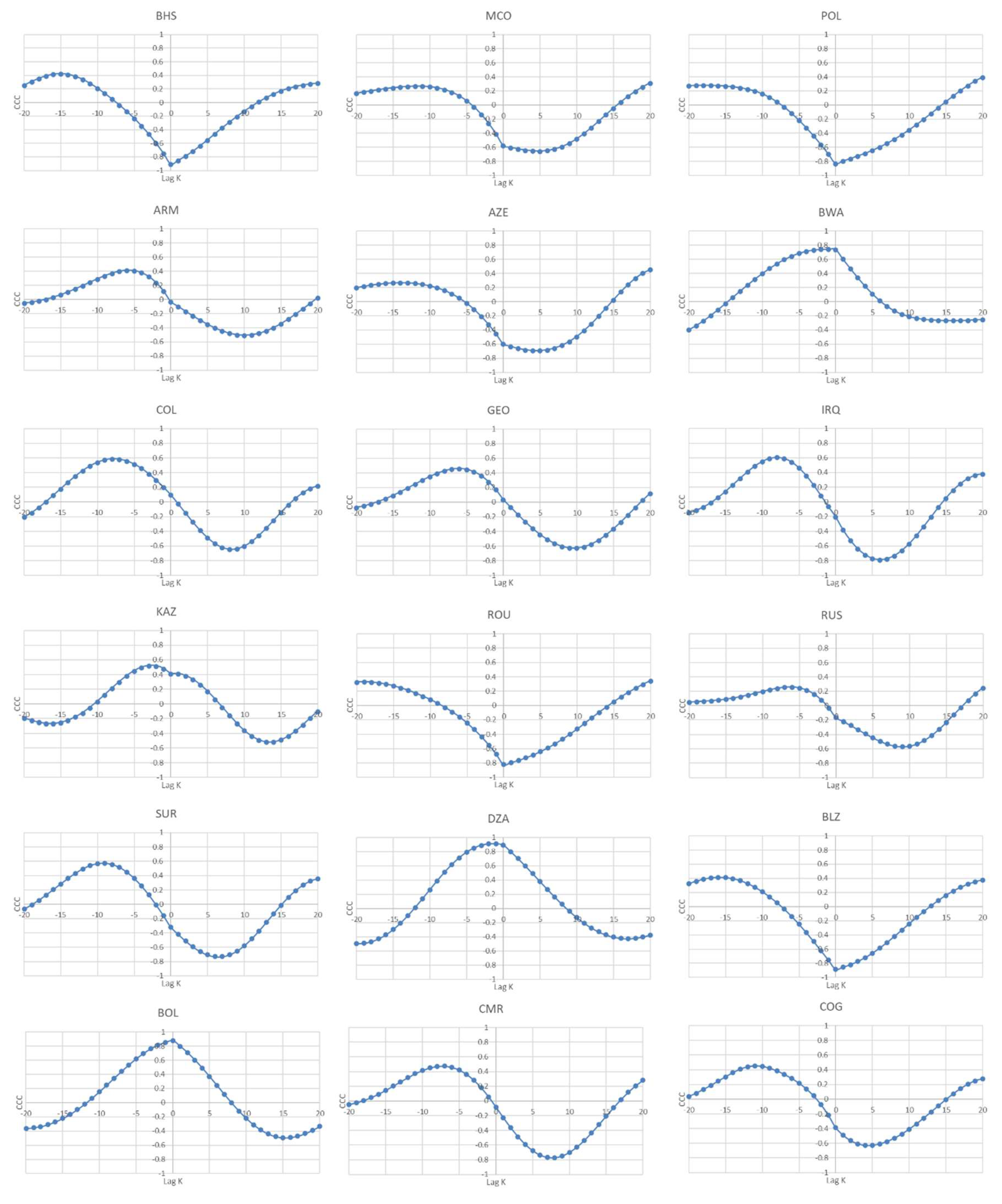
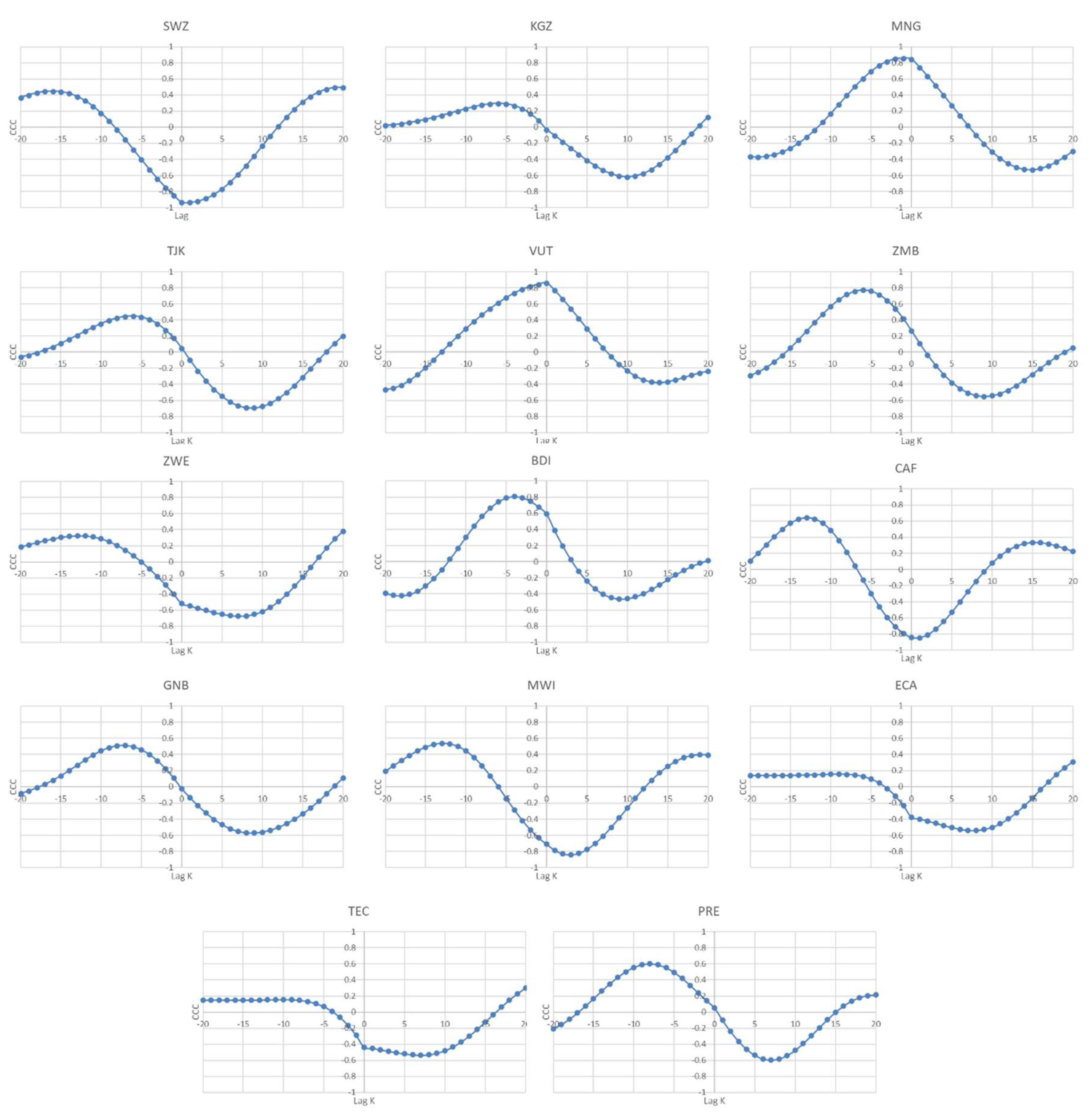
Figure 2.
Plots of the cross-correlation coefficient (CCC) for countries/regions which are in partial agreement with the EKC hypothesis. Note: (i) negative/positive values correspond, respectively, to the lags (past)/leads(future); (ii) were countries/regions in partial agreement with the EKC hypothesis, the ones that display negative sign (-) for the average CCC for the leads are those where an increase in income will reduce (expectantly) CO2 emissions in the future.
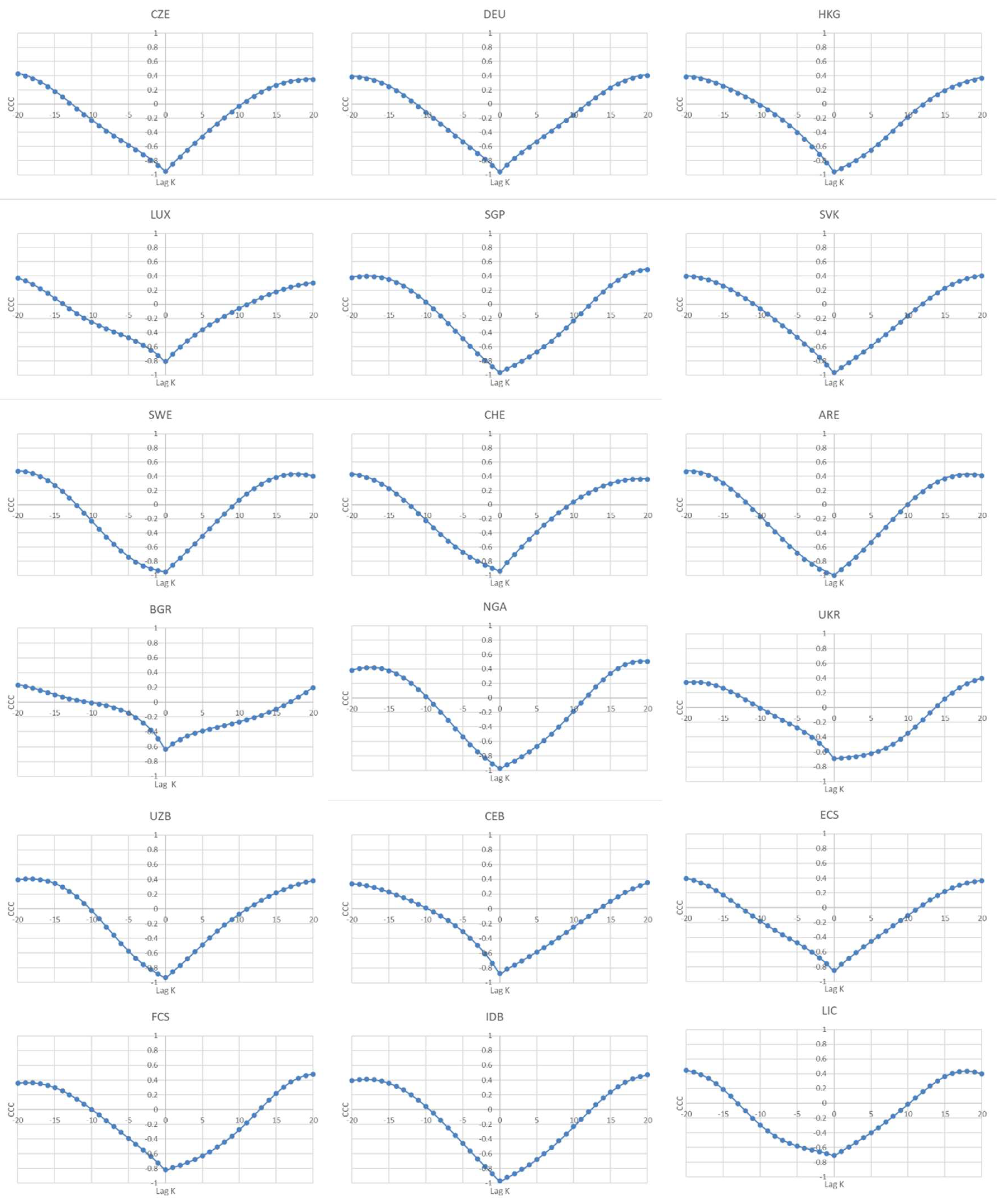

Table 1.
Classification of countries by income level.
| Country categories (Panels) | Acronym | GNI (US$) | Number of countries by category |
|---|---|---|---|
| High income | H | > 12.695 | 47 |
| Upper-middle income | UM | 4.096–12.695 | 44 |
| Lower-middle income | LM | 1.046–4.095 | 49 |
| Low income | L | ≤ 1.045 | 18 |
Table 2.
Summary and descriptive statistics for the panel of high-income (H) countries.
| Country | Code | GDP | CO2 emissions | |||||
|---|---|---|---|---|---|---|---|---|
| Mean | Std.Dev. | Mean | Std.Dev. | Corr. | t-statistic | |||
| Andorra | AND | 33513.756 | 12730.017 | 6.991 | 0.490 | −0.458 | −2.773 | *** |
| Antigua and Barbuda | ATG | 12606.951 | 3440.824 | 4.598 | 0.810 | 0.955 | 17.249 | *** |
| Australia | AUS | 37398.457 | 17743.386 | 16.917 | 1.153 | 0.003 | 0.018 | |
| Austria | AUT | 37669.077 | 11201.962 | 7.948 | 0.671 | −0.160 | −0.872 | |
| Bahamas, The | BHS | 23617.698 | 7225.189 | 6.170 | 0.647 | −0.491 | −3.039 | *** |
| Bahrain | BHR | 16955.385 | 6683.277 | 22.059 | 0.870 | −0.034 | −0.184 | |
| Barbados | BRB | 13513.067 | 3910.232 | 4.526 | 0.676 | 0.681 | 5.003 | *** |
| Belgium | BEL | 35184.785 | 10319.811 | 10.040 | 1.391 | −0.875 | −9.748 | *** |
| Brunei Darussalam | BRN | 25144.941 | 10539.514 | 16.086 | 2.534 | 0.685 | 5.067 | *** |
| Canada | CAN | 34749.151 | 12273.542 | 15.834 | 0.826 | 0.058 | 0.313 | |
| Chile | CHL | 8897.364 | 4712.158 | 3.641 | 0.845 | 0.945 | 15.542 | *** |
| Czechia | CZE | 13257.629 | 7453.118 | 11.342 | 1.448 | −0.814 | −7.558 | *** |
| Denmark | DNK | 45961.280 | 13673.947 | 9.186 | 2.439 | −0.786 | −6.842 | *** |
| Finland | FIN | 36981.853 | 11611.069 | 10.455 | 1.791 | −0.514 | −3.223 | *** |
| France | FRA | 32848.105 | 8406.669 | 5.564 | 0.675 | −0.755 | −6.203 | *** |
| Germany | DEU | 35496.418 | 9128.758 | 9.855 | 1.029 | −0.838 | −8.275 | *** |
| Greece | GRC | 18240.602 | 6296.672 | 7.683 | 1.214 | 0.187 | 1.023 | |
| Hong Kong SAR, China | HKG | 30551.181 | 9719.464 | 5.233 | 0.582 | −0.822 | −7.767 | *** |
| Iceland | ISL | 44024.655 | 15999.350 | 6.845 | 1.212 | −0.708 | −5.400 | *** |
| Ireland | IRL | 43305.016 | 21700.216 | 9.292 | 1.401 | −0.437 | −2.619 | ** |
| Italy | ITA | 28779.928 | 6980.172 | 6.865 | 1.001 | −0.344 | −1.973 | * |
| Japan | JPN | 37999.932 | 4955.627 | 9.187 | 0.396 | 0.204 | 1.120 | |
| Korea, Rep. | KOR | 19019.393 | 8642.434 | 9.940 | 1.841 | 0.913 | 12.061 | *** |
| Kuwait | KWT | 28096.194 | 13518.981 | 23.522 | 5.081 | 0.584 | 3.873 | *** |
| Luxembourg | LUX | 80509.712 | 33061.083 | 21.268 | 4.711 | −0.587 | −3.902 | *** |
| Malta | MLT | 17272.450 | 8152.843 | 5.696 | 1.282 | −0.724 | −5.647 | *** |
| Monaco | MCO | 135307.698 | 45555.805 | 3.585 | 1.829 | −0.433 | −2.590 | ** |
| Netherlands | NLD | 39411.272 | 12443.167 | 9.900 | 0.788 | −0.675 | −4.920 | *** |
| New Zealand | NZL | 26995.219 | 11864.834 | 7.232 | 0.605 | −0.171 | −0.932 | |
| Norway | NOR | 61278.249 | 26302.374 | 7.710 | 0.516 | 0.045 | 0.243 | |
| Oman | OMN | 13526.097 | 6821.440 | 12.861 | 3.694 | 0.920 | 12.600 | *** |
| Poland | POL | 8593.375 | 4888.651 | 8.191 | 0.543 | −0.607 | −4.111 | *** |
| Portugal | PRT | 16996.778 | 5512.428 | 5.089 | 0.670 | −0.102 | −0.552 | |
| Qatar | QAT | 47103.477 | 28177.851 | 38.361 | 5.684 | −0.177 | −0.968 | |
| Saudi Arabia | SAU | 14270.104 | 6556.716 | 13.351 | 2.091 | 0.937 | 14.440 | *** |
| Seychelles | SYC | 10653.678 | 3435.597 | 4.314 | 1.172 | 0.906 | 11.512 | *** |
| Singapore | SGP | 36894.723 | 17488.764 | 9.076 | 1.038 | −0.806 | −7.337 | *** |
| Slovak Republic | SVK | 11405.345 | 6464.644 | 7.034 | 1.124 | −0.868 | −9.392 | *** |
| Spain | ESP | 23038.405 | 7321.656 | 6.241 | 0.974 | −0.042 | −0.225 | |
| St. Kitts and Nevis | KNA | 13298.978 | 5711.927 | 4.223 | 0.804 | 0.917 | 12.393 | *** |
| Sweden | SWE | 42712.338 | 12272.594 | 5.342 | 1.162 | −0.859 | −9.033 | *** |
| Switzerland | CHE | 61599.929 | 19686.175 | 5.694 | 0.730 | −0.866 | −9.306 | *** |
| Trinidad and Tobago | TTO | 11092.989 | 6105.806 | 11.292 | 3.038 | 0.886 | 10.303 | *** |
| United Arab Emirates | ARE | 35667.627 | 7996.840 | 24.926 | 4.130 | −0.796 | −7.086 | *** |
| United Kingdom | GBR | 34866.662 | 9954.021 | 8.046 | 1.554 | −0.658 | −4.712 | *** |
| United States | USA | 43131.007 | 12689.830 | 17.986 | 2.094 | −0.855 | −8.884 | *** |
| Uruguay | URY | 9796.516 | 5645.954 | 1.782 | 0.326 | 0.671 | 4.876 | *** |
Note: (i) “***”, “**” and "*” correspond to the statistical significance at 1%, 5% and 10% significance levels, respectively; (ii) “Std.Dev.” corresponds to the standard deviation; (iii) “Corr.” corresponds to the unconditional correlation between both variables.
Table 3.
Summary and descriptive statistics for the panel of upper middle-income (UM) countries.
| Country | Code | GDP | CO2 emissions | |||||
|---|---|---|---|---|---|---|---|---|
| Mean | Std.Dev. | Mean | Std.Dev. | Corr. | t-statistic | |||
| Albania | ALB | 2665.109 | 1800.928 | 1.298 | 0.444 | 0.804 | 7.282 | *** |
| Argentina | ARG | 8518.593 | 3227.707 | 3.715 | 0.411 | 0.786 | 6.852 | *** |
| Armenia | ARM | 2123.591 | 1619.682 | 1.812 | 1.141 | 0.054 | 0.291 | |
| Azerbaijan | AZE | 2930.402 | 2657.006 | 3.901 | 1.439 | −0.433 | −2.590 | ** |
| Botswana | BWA | 4690.513 | 1590.257 | 2.280 | 0.423 | 0.430 | 2.567 | ** |
| Brazil | BRA | 6549.213 | 3415.845 | 1.837 | 0.328 | 0.857 | 8.942 | *** |
| Bulgaria | BGR | 4718.178 | 3114.510 | 6.182 | 0.642 | −0.306 | −1.730 | * |
| China | CHN | 3620.801 | 3476.529 | 4.655 | 2.182 | 0.945 | 15.529 | *** |
| Colombia | COL | 4277.592 | 2226.098 | 1.543 | 0.125 | 0.198 | 1.089 | |
| Costa Rica | CRI | 6470.315 | 3710.129 | 1.419 | 0.200 | 0.737 | 5.870 | *** |
| Dominica | DMA | 5740.121 | 1653.786 | 1.895 | 0.612 | 0.928 | 13.457 | *** |
| Dominican Republic | DOM | 4227.287 | 2222.225 | 1.961 | 0.376 | 0.724 | 5.645 | *** |
| Ecuador | ECU | 3632.565 | 1851.646 | 2.060 | 0.340 | 0.874 | 9.678 | *** |
| Equatorial Guinea | GNQ | 7175.954 | 6775.226 | 3.837 | 1.786 | 0.708 | 5.405 | *** |
| Fiji | FJI | 3441.352 | 1376.748 | 1.144 | 0.204 | 0.731 | 5.770 | *** |
| Gabon | GAB | 6318.011 | 2019.434 | 3.803 | 0.892 | −0.785 | −6.820 | *** |
| Georgia | GEO | 2342.236 | 1625.935 | 2.097 | 1.365 | 0.117 | 0.634 | |
| Grenada | GRD | 5909.886 | 2169.873 | 2.021 | 0.462 | 0.922 | 12.842 | *** |
| Guatemala | GTM | 2490.587 | 1210.400 | 0.805 | 0.195 | 0.856 | 8.910 | *** |
| Guyana | GUY | 2956.967 | 2353.561 | 2.331 | 0.569 | 0.837 | 8.226 | *** |
| Iraq | IRQ | 3077.271 | 2547.821 | 3.702 | 0.681 | −0.099 | −0.536 | |
| Jamaica | JAM | 3971.723 | 1238.576 | 3.310 | 0.616 | −0.371 | −2.153 | ** |
| Jordan | JOR | 2696.632 | 1223.568 | 2.946 | 0.354 | −0.429 | −2.558 | ** |
| Kazakhstan | KAZ | 5512.682 | 4348.579 | 11.822 | 2.339 | 0.459 | 2.785 | *** |
| Libya | LBY | 8345.772 | 2814.005 | 8.323 | 1.018 | 0.313 | 1.772 | * |
| Malaysia | MYS | 6631.129 | 3043.872 | 5.963 | 1.403 | 0.896 | 10.872 | *** |
| Maldives | MDV | 5069.865 | 3375.597 | 2.132 | 0.954 | 0.970 | 21.379 | *** |
| Marshall Islands | MHL | 2915.601 | 1028.386 | 2.206 | 0.773 | 0.773 | 6.566 | *** |
| Mauritius | MUS | 6343.081 | 3021.857 | 2.328 | 0.752 | 0.940 | 14.778 | *** |
| Mexico | MEX | 8056.363 | 2420.964 | 3.809 | 0.303 | 0.653 | 4.646 | *** |
| North Macedonia | MKD | 3519.998 | 1618.463 | 4.119 | 0.412 | −0.633 | −4.408 | *** |
| Panama | PAN | 7398.370 | 4574.470 | 2.075 | 0.521 | 0.848 | 8.625 | *** |
| Paraguay | PRY | 3421.072 | 1963.058 | 0.835 | 0.207 | 0.779 | 6.680 | *** |
| Peru | PER | 3746.250 | 2082.419 | 1.281 | 0.319 | 0.969 | 21.244 | *** |
| Romania | ROU | 5752.380 | 4257.793 | 4.486 | 0.868 | −0.634 | −4.414 | *** |
| Russian Federation | RUS | 6902.982 | 4683.833 | 11.461 | 1.068 | 0.018 | 0.099 | |
| South Africa | ZAF | 5226.971 | 1825.468 | 7.108 | 0.890 | 0.853 | 8.791 | *** |
| St. Lucia | LCA | 7379.675 | 2389.200 | 2.430 | 0.496 | 0.905 | 11.485 | *** |
| St. Vincent and the Grenadines | VCT | 5227.806 | 2141.860 | 1.781 | 0.558 | 0.915 | 12.199 | *** |
| Suriname | SUR | 4408.957 | 2894.728 | 3.911 | 0.901 | −0.132 | −0.715 | |
| Thailand | THA | 3857.679 | 1909.120 | 3.103 | 0.658 | 0.833 | 8.109 | *** |
| Turkiye | TUR | 6980.295 | 3622.281 | 3.695 | 0.814 | 0.889 | 10.438 | *** |
| Turkmenistan | TKM | 3117.179 | 2706.998 | 9.776 | 1.692 | 0.664 | 4.786 | *** |
| Tuvalu | TUV | 2481.515 | 1242.141 | 0.859 | 0.148 | −0.149 | −0.814 | |
Note: (i) “***”, “**” and "*” correspond to the statistical significance at 1%, 5% and 10% significance levels, respectively; (ii) “Std.Dev.” corresponds to the standard deviation; (iii) “Corr.” corresponds to the unconditional correlation between both variables.
Table 4.
Summary and descriptive statistics for the panel of lower middle-income (LM) countries.
| Country | Code | GDP | CO2 emissions | |||||
|---|---|---|---|---|---|---|---|---|
| Mean | Std.Dev. | Mean | Std.Dev. | Corr. | t-statistic | |||
| Algeria | DZA | 3136.814 | 1432.914 | 3.061 | 0.542 | 0.817 | 7.616 | *** |
| Angola | AGO | 1982.430 | 1586.901 | 0.888 | 0.169 | 0.226 | 1.251 | |
| Bangladesh | BGD | 774.193 | 588.449 | 0.281 | 0.154 | 0.944 | 15.452 | *** |
| Belize | BLZ | 4962.751 | 929.042 | 1.742 | 0.228 | −0.615 | −4.201 | *** |
| Benin | BEN | 775.224 | 344.346 | 0.340 | 0.198 | 0.951 | 16.531 | *** |
| Bolivia | BOL | 1679.277 | 990.356 | 1.359 | 0.328 | 0.842 | 8.390 | *** |
| Cabo Verde | CPV | 2337.745 | 1192.087 | 0.803 | 0.227 | 0.868 | 9.416 | *** |
| Cameroon | CMR | 1173.040 | 320.181 | 0.361 | 0.068 | 0.040 | 0.214 | |
| Comoros | COM | 1136.511 | 327.103 | 0.232 | 0.076 | 0.653 | 4.638 | *** |
| Congo, Rep. | COG | 1838.393 | 998.058 | 1.135 | 0.148 | −0.005 | −0.026 | |
| Cote d'Ivoire | CIV | 1432.329 | 506.953 | 0.326 | 0.069 | 0.703 | 5.325 | *** |
| Djibouti | DJI | 1321.574 | 779.032 | 0.486 | 0.055 | −0.690 | −5.132 | *** |
| Egypt, Arab Rep. | EGY | 1814.874 | 960.204 | 1.934 | 0.350 | 0.812 | 7.494 | *** |
| El Salvador | SLV | 2564.978 | 1034.958 | 0.983 | 0.200 | 0.776 | 6.625 | *** |
| Eswatini | SWZ | 2666.611 | 1105.311 | 1.015 | 0.190 | −0.702 | −5.304 | *** |
| Ghana | GHA | 990.185 | 732.772 | 0.340 | 0.138 | 0.930 | 13.615 | *** |
| Haiti | HTI | 881.238 | 425.613 | 0.206 | 0.071 | 0.921 | 12.689 | *** |
| Honduras | HND | 1522.123 | 590.852 | 0.867 | 0.212 | 0.765 | 6.400 | *** |
| India | IND | 944.063 | 604.968 | 1.133 | 0.380 | 0.986 | 31.738 | *** |
| Indonesia | IDN | 1990.622 | 1323.478 | 1.519 | 0.390 | 0.909 | 11.776 | *** |
| Kenya | KEN | 860.717 | 562.280 | 0.290 | 0.061 | 0.927 | 13.351 | *** |
| Kiribati | KIR | 1104.692 | 386.045 | 0.476 | 0.104 | 0.754 | 6.184 | *** |
| Kyrgyz Republic | KGZ | 735.667 | 393.812 | 1.624 | 0.976 | 0.079 | 0.425 | |
| Lao PDR | LAO | 988.265 | 866.027 | 0.676 | 0.897 | 0.902 | 11.226 | *** |
| Lesotho | LSO | 762.700 | 309.704 | 0.970 | 0.155 | 0.859 | 9.035 | *** |
| Mauritania | MRT | 1223.134 | 459.310 | 0.547 | 0.153 | 0.830 | 7.999 | *** |
| Micronesia, Fed. Sts. | FSM | 2445.629 | 614.171 | 1.292 | 0.421 | 0.018 | 0.099 | |
| Mongolia | MNG | 1946.519 | 1588.169 | 5.102 | 1.162 | 0.802 | 7.225 | *** |
| Morocco | MAR | 2345.155 | 867.836 | 1.396 | 0.317 | 0.967 | 20.350 | *** |
| Myanmar | MMR | 582.229 | 527.164 | 0.254 | 0.164 | 0.763 | 6.358 | *** |
| Nepal | NPL | 490.987 | 347.138 | 0.183 | 0.143 | 0.933 | 13.921 | *** |
| Nicaragua | NIC | 1261.086 | 549.009 | 0.715 | 0.125 | 0.737 | 5.873 | *** |
| Nigeria | NGA | 1601.920 | 829.271 | 0.686 | 0.122 | −0.695 | −5.211 | *** |
| Pakistan | PAK | 873.978 | 417.101 | 0.694 | 0.102 | 0.915 | 12.222 | *** |
| Papua New Guinea | PNG | 1493.388 | 791.845 | 0.615 | 0.097 | 0.551 | 3.553 | *** |
| Philippines | PHL | 1812.246 | 892.837 | 0.925 | 0.174 | 0.758 | 6.253 | *** |
| Samoa | WSM | 2537.854 | 1294.011 | 0.898 | 0.199 | 0.892 | 10.602 | *** |
| Senegal | SEN | 1059.197 | 308.972 | 0.491 | 0.134 | 0.825 | 7.849 | *** |
| Solomon Islands | SLB | 1465.966 | 579.793 | 0.546 | 0.076 | −0.146 | −0.795 | |
| Sri Lanka | LKA | 1981.855 | 1442.738 | 0.635 | 0.252 | 0.889 | 10.473 | *** |
| Tajikistan | TJK | 525.295 | 317.412 | 0.617 | 0.432 | 0.102 | 0.550 | |
| Tanzania | TZA | 564.769 | 319.562 | 0.137 | 0.058 | 0.961 | 18.803 | *** |
| Tunisia | TUN | 2998.875 | 992.619 | 2.250 | 0.316 | 0.931 | 13.781 | *** |
| Ukraine | UKR | 2115.424 | 1183.604 | 6.610 | 2.278 | −0.396 | −2.322 | ** |
| Uzbekistan | UZB | 1175.693 | 790.401 | 4.412 | 0.726 | −0.823 | −7.798 | *** |
| Vanuatu | VUT | 2063.623 | 716.584 | 0.451 | 0.079 | 0.483 | 2.968 | *** |
| Viet Nam | VNM | 1257.278 | 1157.203 | 1.322 | 0.959 | 0.973 | 22.813 | *** |
| Zambia | ZMB | 900.692 | 521.524 | 0.261 | 0.084 | 0.226 | 1.252 | |
| Zimbabwe | ZWE | 876.170 | 442.966 | 1.024 | 0.357 | −0.337 | −1.930 | * |
Note: (i) “***”, “**” and "*” correspond to the statistical significance at 1%, 5% and 10% significance levels, respectively; (ii) “Std.Dev.” corresponds to the standard deviation; (iii) “Corr.” corresponds to the unconditional correlation between both variables.
Table 5.
Summary and descriptive statistics for the panel of low-income (L) countries.
| Country | Code | GDP | CO2 emissions | |||||
|---|---|---|---|---|---|---|---|---|
| Mean | Std.Dev. | Mean | Std.Dev. | Corr. | t-statistic | |||
| Burkina Faso | BFA | 483.356 | 211.656 | 0.123 | 0.065 | 0.873 | 9.628 | *** |
| Burundi | BDI | 189.134 | 46.069 | 0.036 | 0.010 | 0.376 | 2.182 | ** |
| Central African Republic | CAF | 372.932 | 87.692 | 0.049 | 0.010 | −0.574 | −3.779 | *** |
| Chad | TCD | 538.884 | 305.413 | 0.081 | 0.017 | 0.882 | 10.068 | *** |
| Ethiopia | ETH | 334.374 | 249.384 | 0.080 | 0.039 | 0.945 | 15.608 | *** |
| Gambia, The | GMB | 620.288 | 122.167 | 0.209 | 0.030 | 0.417 | 2.469 | ** |
| Guinea | GIN | 587.920 | 207.676 | 0.207 | 0.052 | 0.834 | 8.146 | *** |
| Guinea-Bissau | GNB | 438.391 | 194.574 | 0.155 | 0.015 | 0.002 | 0.012 | |
| Madagascar | MDG | 386.385 | 99.034 | 0.099 | 0.020 | 0.576 | 3.793 | *** |
| Malawi | MWI | 425.618 | 157.423 | 0.077 | 0.008 | −0.477 | −2.921 | *** |
| Mali | MLI | 518.234 | 231.972 | 0.120 | 0.049 | 0.935 | 14.198 | *** |
| Niger | NER | 380.385 | 132.584 | 0.071 | 0.019 | 0.813 | 7.528 | *** |
| Rwanda | RWA | 446.082 | 227.983 | 0.079 | 0.015 | 0.615 | 4.204 | *** |
| Sierra Leone | SLE | 340.939 | 170.745 | 0.098 | 0.033 | 0.894 | 10.773 | *** |
| Sudan | SDN | 1122.105 | 782.028 | 0.351 | 0.133 | 0.741 | 5.942 | *** |
| Togo | TGO | 548.882 | 234.301 | 0.273 | 0.064 | 0.326 | 1.854 | * |
| Uganda | UGA | 483.754 | 278.287 | 0.082 | 0.035 | 0.937 | 14.498 | *** |
| Yemen, Rep. | YEM | 931.176 | 398.789 | 0.735 | 0.246 | 0.105 | 0.570 | |
Note: (i) “***”, “**” and "*” correspond to the statistical significance at 1%, 5% and 10% significance levels, respectively; (ii) “Std.Dev.” corresponds to the standard deviation; (iii) “Corr.” corresponds to the unconditional correlation between both variables.
Table 6.
Summary and descriptive statistics for the world regions.
| World region | Code | GDP | CO2 emissions | |||||
|---|---|---|---|---|---|---|---|---|
| Mean | Std. Dev. | Mean | Std.Dev. | Corr. | t-statistic | |||
| Arab World | ARB | 4409.764 | 1994.329 | 3.687 | 0.551 | 0.958 | 18.087 | *** |
| Caribbean small states | CSS | 7079.385 | 2907.295 | 4.930 | 0.592 | 0.797 | 7.101 | *** |
| Central Europe and the Baltics | CEB | 8716.471 | 5125.355 | 6.933 | 0.641 | −0.677 | −4.953 | *** |
| Early-demographic dividend | EAR | 2145.871 | 997.383 | 1.758 | 0.324 | 0.983 | 29.132 | *** |
| East Asia & Pacific | EAS | 6277.222 | 2971.174 | 4.279 | 1.426 | 0.965 | 19.857 | *** |
| East Asia & Pacific (excluding high-income) | EAP | 3102.089 | 2735.300 | 3.707 | 1.582 | 0.953 | 17.009 | *** |
| East Asia & Pacific (IDA & IBRD countries) | TEA | 3137.219 | 2765.625 | 3.719 | 1.614 | 0.953 | 16.953 | *** |
| Euro area | EMU | 30041.323 | 8329.311 | 7.521 | 0.813 | −0.701 | −5.290 | *** |
| Europe & Central Asia | ECS | 18426.500 | 6185.380 | 7.558 | 0.741 | −0.664 | −4.787 | *** |
| Europe & Central Asia (excluding high-income) | ECA | 5074.851 | 3165.363 | 7.606 | 0.940 | −0.156 | −0.850 | |
| Europe & Central Asia (IDA & IBRD countries) | TEC | 5449.408 | 3331.387 | 7.473 | 0.857 | −0.220 | −1.213 | |
| European Union | EUU | 26145.894 | 7939.703 | 7.460 | 0.770 | −0.752 | −6.151 | *** |
| Fragile and conflict-affected situations | FCS | 1426.060 | 602.529 | 1.282 | 0.335 | −0.645 | −4.540 | *** |
| Heavily indebted poor countries (HIPC) | HPC | 632.022 | 278.419 | 0.205 | 0.046 | 0.973 | 22.850 | *** |
| High income | HIC | 32361.412 | 8926.937 | 10.915 | 0.730 | −0.660 | −4.728 | *** |
| IBRD only | IBD | 3222.182 | 2068.898 | 3.339 | 0.791 | 0.987 | 33.038 | *** |
| IDA & IBRD total | IBT | 2652.901 | 1627.332 | 2.667 | 0.556 | 0.985 | 31.048 | *** |
| IDA blend | IDB | 1183.662 | 567.481 | 0.897 | 0.067 | −0.901 | −11.179 | *** |
| IDA only | IDX | 744.650 | 324.124 | 0.289 | 0.060 | 0.968 | 20.673 | *** |
| IDA total | IDA | 890.843 | 399.954 | 0.491 | 0.025 | 0.747 | 6.049 | *** |
| Late-demographic dividend | LTE | 4487.925 | 3304.814 | 4.735 | 1.390 | 0.982 | 27.865 | *** |
| Latin America & Caribbean | LCN | 6267.761 | 2639.431 | 2.443 | 0.260 | 0.897 | 10.935 | *** |
| Latin America & Caribbean (excluding high-income) | LAC | 5966.245 | 2463.491 | 2.258 | 0.238 | 0.912 | 11.967 | *** |
| Latin America & the Caribbean (IDA & IBRD countries) | TLA | 6169.196 | 2624.209 | 2.459 | 0.265 | 0.897 | 10.910 | *** |
| Least developed countries: UN classification | LDC | 620.251 | 326.348 | 0.218 | 0.074 | 0.957 | 17.747 | *** |
| Low & middle income | LMY | 2540.821 | 1573.965 | 2.599 | 0.568 | 0.985 | 30.271 | *** |
| Low income | LIC | 649.790 | 214.273 | 0.394 | 0.094 | −0.386 | −2.252 | ** |
| Lower middle income | LMC | 1210.648 | 676.003 | 1.283 | 0.222 | 0.980 | 26.532 | *** |
| Middle East & North Africa | MEA | 5109.302 | 2336.851 | 4.648 | 0.749 | 0.956 | 17.448 | *** |
| Middle East & North Africa (excluding high-income) | MNA | 2817.581 | 1229.723 | 3.156 | 0.442 | 0.914 | 12.099 | *** |
| Middle East & North Africa (IDA & IBRD countries) | TMN | 2825.307 | 1235.171 | 3.190 | 0.449 | 0.913 | 12.054 | *** |
| Middle income | MIC | 2730.098 | 1733.156 | 2.807 | 0.654 | 0.986 | 31.420 | *** |
| North America | NAC | 42300.725 | 12518.295 | 17.770 | 1.927 | −0.837 | −8.239 | *** |
| OECD members | OED | 29249.160 | 7759.829 | 9.912 | 0.773 | −0.725 | −5.669 | *** |
| Other small states | OSS | 8366.543 | 4673.966 | 5.300 | 0.742 | 0.972 | 22.326 | *** |
| Pacific island small states | PSS | 2619.201 | 952.894 | 1.020 | 0.112 | 0.505 | 3.152 | *** |
| Post-demographic dividend | PST | 33151.302 | 9035.017 | 11.068 | 0.906 | −0.755 | −6.203 | *** |
| Pre-demographic dividend | PRE | 1009.993 | 490.465 | 0.474 | 0.040 | 0.065 | 0.353 | |
| Small states | SST | 7761.159 | 4095.455 | 4.950 | 0.666 | 0.968 | 20.902 | *** |
| South Asia | SAS | 916.023 | 574.025 | 0.968 | 0.313 | 0.988 | 33.776 | *** |
| Sub-Saharan Africa | SSF | 1177.861 | 470.510 | 0.768 | 0.029 | −0.030 | −0.162 | |
| Sub-Saharan Africa (excluding high income) | SSA | 1176.860 | 470.380 | 0.768 | 0.029 | −0.032 | −0.171 | |
| Upper middle income | UMC | 4323.453 | 2930.511 | 4.360 | 1.210 | 0.981 | 27.082 | *** |
| World | WLD | 7700.699 | 2545.740 | 4.263 | 0.322 | 0.945 | 15.611 | *** |
Notes: (i) “***”, “**” and "*” correspond to the statistical significance at 1%, 5% and 10% significance levels, respectively; (ii) “Std.Dev.” corresponds to the standard deviation; (iii) “Corr.” corresponds to the unconditional correlation between both variables.
Table 7.
Cross-correlation coefficient results for the panel of high-income (H) countries.
| Country | Code | Lags | Leads | (Aver. CCC lags)/(Aver. CCC leads) | |||||
|---|---|---|---|---|---|---|---|---|---|
| Σ of CCC | Aver. CCC | Σ of CCC | Aver. CCC | (+)/(-) | (-)/(-) | (-)/(+) | (+)/(+) | ||
| Andorra | AND | −7.042 | −0.352 | 3.093 | 0.155 | X | |||
| Antigua and Barbuda | ATG | 1.640 | 0.082 | 3.098 | 0.155 | X | |||
| Australia | AUS | −6.409 | −0.320 | 6.783 | 0.339 | X | |||
| Austria | AUT | −7.123 | −0.356 | 5.411 | 0.271 | X | |||
| Bahamas, The | BHS | 1.416 | 0.071 | −3.417 | −0.171 | X | |||
| Bahrain | BHR | −5.458 | −0.273 | 6.009 | 0.300 | X | |||
| Barbados | BRB | −2.998 | −0.150 | 4.982 | 0.249 | X | |||
| Belgium | BEL | −4.467 | −0.223 | 0.149 | 0.007 | X | |||
| Brunei Darussalam | BRN | 1.482 | 0.074 | 1.873 | 0.094 | X | |||
| Canada | CAN | −6.774 | −0.339 | 6.410 | 0.320 | X | |||
| Chile | CHL | 1.603 | 0.080 | 3.273 | 0.164 | X | |||
| Czechia | CZE | −3.458 | −0.173 | −1.595 | −0.080 | X | |||
| Denmark | DNK | −4.665 | −0.233 | 0.072 | 0.004 | X | |||
| Finland | FIN | −6.599 | −0.330 | 2.805 | 0.140 | X | |||
| France | FRA | −5.332 | −0.267 | 0.943 | 0.047 | X | |||
| Germany | DEU | −2.401 | −0.120 | −2.587 | −0.129 | X | |||
| Greece | GRC | −8.195 | −0.410 | 4.505 | 0.225 | X | |||
| Hong Kong SAR, China | HKG | −1.112 | −0.056 | −3.821 | −0.191 | X | |||
| Iceland | ISL | −5.115 | −0.256 | 0.536 | 0.027 | X | |||
| Ireland | IRL | −5.985 | −0.299 | 3.257 | 0.163 | X | |||
| Italy | ITA | −7.367 | −0.368 | 3.658 | 0.183 | X | |||
| Japan | JPN | −6.023 | −0.301 | 4.230 | 0.211 | X | |||
| Korea, Rep. | KOR | 0.578 | 0.029 | 4.455 | 0.223 | X | |||
| Kuwait | KWT | −4.113 | −0.206 | 4.203 | 0.210 | X | |||
| Luxembourg | LUX | −3.479 | −0.174 | −1.592 | −0.080 | X | |||
| Malta | MLT | −4.985 | −0.249 | 0.753 | 0.038 | X | |||
| Monaco | MCO | 2.582 | 0.129 | −6.264 | −0.313 | X | |||
| Netherlands | NLD | −6.040 | −0.302 | 1.540 | 0.077 | X | |||
| New Zealand | NZL | −6.196 | −0.310 | 6.340 | 0.317 | X | |||
| Norway | NOR | −6.793 | −0.340 | 5.898 | 0.295 | X | |||
| Oman | OMN | 1.103 | 0.055 | 2.717 | 0.136 | X | |||
| Poland | POL | 0.528 | 0.026 | −5.257 | −0.263 | X | |||
| Portugal | PRT | −6.901 | −0.345 | 5.672 | 0.284 | X | |||
| Qatar | QAT | −6.852 | −0.343 | 5.832 | 0.292 | X | |||
| Saudi Arabia | SAU | 1.557 | 0.078 | 2.515 | 0.126 | X | |||
| Seychelles | SYC | 2.038 | 0.102 | 3.242 | 0.162 | X | |||
| Singapore | SGP | −1.033 | −0.052 | −3.481 | −0.174 | X | |||
| Slovak Republic | SVK | −1.767 | −0.088 | −3.144 | −0.157 | X | |||
| Spain | ESP | −7.544 | −0.377 | 5.409 | 0.270 | X | |||
| St. Kitts and Nevis | KNA | 0.452 | 0.023 | 4.513 | 0.226 | X | |||
| Sweden | SWE | −3.878 | −0.194 | −0.355 | −0.018 | X | |||
| Switzerland | CHE | −3.793 | −0.190 | −0.711 | −0.036 | X | |||
| Trinidad and Tobago | TTO | 0.151 | 0.008 | 2.131 | 0.107 | X | |||
| United Arab Emirates | ARE | −3.084 | −0.154 | −1.219 | −0.061 | X | |||
| United Kingdom | GBR | −6.325 | −0.316 | 1.431 | 0.072 | X | |||
| United States | USA | −4.803 | −0.240 | 0.309 | 0.015 | X | |||
| Uruguay | URY | −1.334 | −0.067 | 5.689 | 0.284 | X | |||
Notes: (i) “CCC” corresponds to the cross-correlation coefficient estimated according to the method proposed by Narayan et al. (2016); (ii) “Aver.” corresponds to the mean of the CCC.
Table 8.
Cross-correlation coefficient results for the panel of upper middle-income UM) countries.
| Country | Code | Lags | Leads | (Aver. CCC lags)/(Aver. CCC leads) | |||||
|---|---|---|---|---|---|---|---|---|---|
| Σ of CCC | Aver. CCC | Σ of CCC | Aver. CCC | (+)/(-) | (-)/(-) | (-)/(+) | (+)/(+) | ||
| Albania | ALB | 2.572 | 0.129 | 1.421 | 0.071 | X | |||
| Argentina | ARG | −1.809 | −0.090 | 5.497 | 0.275 | X | |||
| Armenia | ARM | 3.980 | 0.199 | −6.273 | −0.314 | X | |||
| Azerbaijan | AZE | 2.142 | 0.107 | −5.760 | −0.288 | X | |||
| Botswana | BWA | 5.719 | 0.286 | −1.355 | −0.068 | X | |||
| Brazil | BRA | 1.226 | 0.061 | 2.794 | 0.140 | X | |||
| Bulgaria | BGR | −0.522 | −0.026 | −4.344 | −0.217 | X | |||
| China | CHN | 0.601 | 0.030 | 3.943 | 0.197 | X | |||
| Colombia | COL | 6.090 | 0.304 | −5.558 | −0.278 | X | |||
| Costa Rica | CRI | −1.143 | −0.057 | 5.850 | 0.292 | X | |||
| Dominica | DMA | 0.782 | 0.039 | 3.851 | 0.193 | X | |||
| Dominican Republic | DOM | −0.984 | −0.049 | 5.961 | 0.298 | X | |||
| Ecuador | ECU | −0.369 | −0.018 | 4.789 | 0.239 | X | |||
| Equatorial Guinea | GNQ | −3.124 | −0.156 | 3.915 | 0.196 | X | |||
| Fiji | FJI | 1.171 | 0.059 | 4.052 | 0.203 | X | |||
| Gabon | GAB | −3.635 | −0.182 | 0.720 | 0.036 | X | |||
| Georgia | GEO | 4.636 | 0.232 | −7.120 | −0.356 | X | |||
| Grenada | GRD | 1.276 | 0.064 | 3.933 | 0.197 | X | |||
| Guatemala | GTM | 0.667 | 0.033 | 4.708 | 0.235 | X | |||
| Guyana | GUY | 2.944 | 0.147 | 1.842 | 0.092 | X | |||
| Iraq | IRQ | 5.283 | 0.264 | −6.099 | −0.305 | X | |||
| Jamaica | JAM | −6.906 | −0.345 | 3.431 | 0.172 | X | |||
| Jordan | JOR | −6.571 | −0.329 | 3.835 | 0.192 | X | |||
| Kazakhstan | KAZ | 1.546 | 0.077 | −2.976 | −0.149 | X | |||
| Libya | LBY | −4.513 | −0.226 | 6.170 | 0.309 | X | |||
| Malaysia | MYS | 0.258 | 0.013 | 4.560 | 0.228 | X | |||
| Maldives | MDV | 1.493 | 0.075 | 3.479 | 0.174 | X | |||
| Marshall Islands | MHL | −0.372 | −0.019 | 5.549 | 0.277 | X | |||
| Mauritius | MUS | 0.781 | 0.039 | 4.087 | 0.204 | X | |||
| Mexico | MEX | −4.029 | −0.201 | 4.495 | 0.225 | X | |||
| North Macedonia | MKD | −4.714 | −0.236 | 1.115 | 0.056 | X | |||
| Panama | PAN | −0.258 | −0.013 | 5.076 | 0.254 | X | |||
| Paraguay | PRY | 3.121 | 0.156 | 1.264 | 0.063 | X | |||
| Peru | PER | 1.919 | 0.096 | 2.436 | 0.122 | X | |||
| Romania | ROU | 0.232 | 0.012 | −5.237 | −0.262 | X | |||
| Russian Federation | RUS | 2.822 | 0.141 | −6.041 | −0.302 | X | |||
| South Africa | ZAF | −0.629 | −0.031 | 3.504 | 0.175 | X | |||
| St. Lucia | LCA | 0.297 | 0.015 | 4.700 | 0.235 | X | |||
| St. Vincent and the Grenadines | VCT | 0.318 | 0.016 | 4.420 | 0.221 | X | |||
| Suriname | SUR | 5.648 | 0.282 | −6.308 | −0.315 | X | |||
| Thailand | THA | −0.578 | −0.029 | 5.583 | 0.279 | X | |||
| Turkiye | TUR | 3.570 | 0.179 | 0.906 | 0.045 | X | |||
| Turkmenistan | TKM | −0.722 | −0.036 | 3.844 | 0.192 | X | |||
| Tuvalu | TUV | −6.195 | −0.310 | 5.766 | 0.288 | X | |||
Notes: (i) “CCC” corresponds to the cross-correlation coefficient estimated according to the method proposed by Narayan et al. (2016); (ii) “Aver.” corresponds to the mean of the CCC.
Table 9.
Cross-correlation coefficient results for lower middle-income (LM) countries.
| Country | Code | Lags | Leads | (Aver. CCC lags)/(Aver. CCC leads) | |||||
|---|---|---|---|---|---|---|---|---|---|
| Σ of CCC | Aver. CCC | Σ of CCC | Aver. CCC | (+)/(-) | (-)/(-) | (-)/(+) | (+)/(+) | ||
| Algeria | DZA | 4.102 | 0.205 | −0.346 | −0.017 | X | |||
| Angola | AGO | −4.264 | −0.213 | 5.273 | 0.264 | X | |||
| Bangladesh | BGD | 0.686 | 0.034 | 3.729 | 0.186 | X | |||
| Belize | BLZ | 1.398 | 0.070 | −4.353 | −0.218 | X | |||
| Benin | BEN | 2.272 | 0.114 | 2.525 | 0.126 | X | |||
| Bolivia | BOL | 3.386 | 0.169 | −1.245 | −0.062 | X | |||
| Cabo Verde | CPV | 0.743 | 0.037 | 3.582 | 0.179 | X | |||
| Cameroon | CMR | 4.937 | 0.247 | −7.669 | −0.383 | X | |||
| Comoros | COM | 2.943 | 0.147 | 1.325 | 0.066 | X | |||
| Congo, Rep. | COG | 4.618 | 0.231 | −5.458 | −0.273 | X | |||
| Cote d'Ivoire | CIV | 1.507 | 0.075 | 3.856 | 0.193 | X | |||
| Djibouti | DJI | −3.880 | −0.194 | 2.471 | 0.124 | X | |||
| Egypt, Arab Rep. | EGY | −0.120 | −0.006 | 4.455 | 0.223 | X | |||
| El Salvador | SLV | −1.105 | −0.055 | 5.670 | 0.283 | X | |||
| Eswatini | SWZ | 0.549 | 0.027 | −3.841 | −0.192 | X | |||
| Ghana | GHA | 1.088 | 0.054 | 3.561 | 0.178 | X | |||
| Haiti | HTI | 2.643 | 0.132 | 2.221 | 0.111 | X | |||
| Honduras | HND | −1.539 | −0.077 | 6.070 | 0.303 | X | |||
| India | IND | 1.776 | 0.089 | 2.878 | 0.144 | X | |||
| Indonesia | IDN | 0.794 | 0.040 | 4.129 | 0.206 | X | |||
| Kenya | KEN | 2.843 | 0.142 | 0.968 | 0.048 | X | |||
| Kiribati | KIR | −0.374 | −0.019 | 4.338 | 0.217 | X | |||
| Kyrgyz Republic | KGZ | 3.337 | 0.167 | −7.047 | −0.352 | X | |||
| Lao PDR | LAO | 3.118 | 0.156 | 0.419 | 0.021 | X | |||
| Lesotho | LSO | 0.641 | 0.032 | 3.001 | 0.150 | X | |||
| Mauritania | MRT | 2.926 | 0.146 | 0.907 | 0.045 | X | |||
| Micronesia, Fed. Sts. | FSM | −2.482 | −0.124 | 4.009 | 0.200 | X | |||
| Mongolia | MNG | 3.658 | 0.183 | −2.346 | −0.117 | X | |||
| Morocco | MAR | 2.354 | 0.118 | 2.396 | 0.120 | X | |||
| Myanmar | MMR | 3.740 | 0.187 | 0.539 | 0.027 | X | |||
| Nepal | NPL | 2.907 | 0.145 | 1.167 | 0.058 | X | |||
| Nicaragua | NIC | −1.402 | −0.070 | 5.709 | 0.285 | X | |||
| Nigeria | NGA | −1.219 | −0.061 | −2.816 | −0.141 | X | |||
| Pakistan | PAK | 1.766 | 0.088 | 3.367 | 0.168 | X | |||
| Papua New Guinea | PNG | −1.266 | −0.063 | 5.309 | 0.265 | X | |||
| Philippines | PHL | 2.785 | 0.139 | 1.786 | 0.089 | X | |||
| Samoa | WSM | 1.870 | 0.094 | 3.248 | 0.162 | X | |||
| Senegal | SEN | 0.628 | 0.031 | 3.601 | 0.180 | X | |||
| Solomon Islands | SLB | −5.705 | −0.285 | 5.866 | 0.293 | X | |||
| Sri Lanka | LKA | 1.283 | 0.064 | 3.779 | 0.189 | X | |||
| Tajikistan | TJK | 4.742 | 0.237 | −7.472 | −0.374 | X | |||
| Tanzania | TZA | 2.741 | 0.137 | 2.177 | 0.109 | X | |||
| Tunisia | TUN | 2.682 | 0.134 | 1.322 | 0.066 | X | |||
| Ukraine | UKR | −0.118 | −0.006 | −4.406 | −0.220 | X | |||
| Uzbekistan | UZB | −1.843 | −0.092 | −2.292 | −0.115 | X | |||
| Vanuatu | VUT | 4.250 | 0.212 | −0.697 | −0.035 | X | |||
| Viet Nam | VNM | 2.030 | 0.102 | 2.504 | 0.125 | X | |||
| Zambia | ZMB | 7.000 | 0.350 | −5.704 | −0.285 | X | |||
| Zimbabwe | ZWE | 2.766 | 0.138 | −7.409 | −0.370 | X | |||
Notes: (i) “CCC” corresponds to the cross-correlation coefficient estimated according to the method proposed by Narayan et al. (2016); (ii) “Aver.” corresponds to the mean of the CCC.
Table 10.
Cross-correlation coefficient results for the panel of low-income (L) countries.
| Country | Code | Lags | Leads | (Aver. CCC lags)/(Aver. CCC leads) | |||||
|---|---|---|---|---|---|---|---|---|---|
| Σ of CCC | Aver. CCC | Σ of CCC | Aver. CCC | (+)/(-) | (-)/(-) | (-)/(+) | (+)/(+) | ||
| Burkina Faso | BFA | 3.388 | 0.169 | 0.836 | 0.042 | X | |||
| Burundi | BDI | 4.111 | 0.206 | −3.874 | −0.194 | X | |||
| Central African Republic | CAF | 2.653 | 0.133 | −1.602 | −0.080 | X | |||
| Chad | TCD | 3.009 | 0.150 | 0.231 | 0.012 | X | |||
| Ethiopia | ETH | 0.550 | 0.027 | 3.212 | 0.161 | X | |||
| Gambia, The | GMB | 1.928 | 0.096 | 1.590 | 0.079 | X | |||
| Guinea | GIN | 0.931 | 0.047 | 3.144 | 0.157 | X | |||
| Guinea-Bissau | GNB | 5.180 | 0.259 | −6.979 | −0.349 | X | |||
| Madagascar | MDG | 3.746 | 0.187 | 0.645 | 0.032 | X | |||
| Malawi | MWI | 3.356 | 0.168 | −4.334 | −0.217 | X | |||
| Mali | MLI | 1.907 | 0.095 | 2.875 | 0.144 | X | |||
| Niger | NER | 1.254 | 0.063 | 1.030 | 0.051 | X | |||
| Rwanda | RWA | 3.432 | 0.172 | 0.806 | 0.040 | X | |||
| Sierra Leone | SLE | 3.057 | 0.153 | 1.047 | 0.052 | X | |||
| Sudan | SDN | 0.858 | 0.043 | 1.852 | 0.093 | X | |||
| Togo | TGO | −3.624 | −0.181 | 7.107 | 0.355 | X | |||
| Uganda | UGA | 2.133 | 0.107 | 2.301 | 0.115 | X | |||
| Yemen, Rep. | YEM | −3.368 | −0.168 | 3.962 | 0.198 | X | |||
Notes: (i) “CCC” corresponds to the cross-correlation coefficient estimated according to the method proposed by Narayan et al. (2016); (ii) “Aver.” corresponds to the mean of the CCC.
Table 11.
Cross-correlation coefficient results for the world regions.
| World region | Code | Lags | Leads | (Aver. CCC lags)/(Aver. CCC leads) | |||||
|---|---|---|---|---|---|---|---|---|---|
| Σ of CCC | Aver. CCC | Σ of CCC | Aver. CCC | (+)/(-) | (-)/(-) | (-)/(+) | (+)/(+) | ||
| Arab World | ARB | 1.4163 | 0.0708 | 2.7020 | 0.1351 | X | |||
| Caribbean small states | CSS | −0.7673 | −0.0384 | 3.3647 | 0.1682 | X | |||
| Central Europe and the Baltics | CEB | −0.7807 | −0.0390 | −4.2701 | −0.2135 | X | |||
| Early-demographic dividend | EAR | 1.7162 | 0.0858 | 2.9637 | 0.1482 | X | |||
| East Asia & Pacific | EAS | 0.9762 | 0.0488 | 3.6751 | 0.1838 | X | |||
| East Asia & Pacific (excluding high-income) | EAP | 0.6940 | 0.0347 | 3.8910 | 0.1945 | X | |||
| East Asia & Pacific (IDA & IBRD countries) | TEA | 0.6817 | 0.0341 | 3.9099 | 0.1955 | X | |||
| Euro area | EMU | −5.7828 | −0.2891 | 1.4026 | 0.0701 | X | |||
| Europe & Central Asia | ECS | −2.8028 | −0.1401 | −2.1610 | −0.1081 | X | |||
| Europe & Central Asia (excluding high-income) | ECA | 1.8913 | 0.0946 | −5.7348 | −0.2867 | X | |||
| Europe & Central Asia (IDA & IBRD countries) | TEC | 1.7816 | 0.0891 | −5.7382 | −0.2869 | X | |||
| European Union | EUU | −5.1135 | −0.2557 | 0.4929 | 0.0246 | X | |||
| Fragile and conflict-affected situations | FCS | −0.8084 | −0.0404 | −3.5588 | −0.1779 | X | |||
| Heavily indebted poor countries (HIPC) | HPC | 2.3229 | 0.1161 | 1.8006 | 0.0900 | X | |||
| High income | HIC | −6.3282 | −0.3164 | 2.5069 | 0.1253 | X | |||
| IBRD only | IBD | 1.6665 | 0.0833 | 2.6546 | 0.1327 | X | |||
| IDA & IBRD total | IBT | 1.6870 | 0.0843 | 2.5757 | 0.1288 | X | |||
| IDA blend | IDB | −0.8144 | −0.0407 | −3.8206 | −0.1910 | X | |||
| IDA only | IDX | 2.6625 | 0.1331 | 1.9562 | 0.0978 | X | |||
| IDA total | IDA | 4.0536 | 0.2027 | 0.1180 | 0.0059 | X | |||
| Late-demographic dividend | LTE | 1.4871 | 0.0744 | 2.8646 | 0.1432 | X | |||
| Latin America & Caribbean | LCN | −0.4408 | −0.0220 | 4.1896 | 0.2095 | X | |||
| Latin America & Caribbean (excluding high-income) | LAC | −0.0048 | −0.0002 | 3.9480 | 0.1974 | X | |||
| Latin America & the Caribbean (IDA & IBRD countries) | TLA | −0.4764 | −0.0238 | 4.2045 | 0.2102 | X | |||
| Least developed countries: UN classification | LDC | 1.9338 | 0.0967 | 2.6043 | 0.1302 | X | |||
| Low & middle income | LMY | 1.6198 | 0.0810 | 2.6587 | 0.1329 | X | |||
| Low income | LIC | −3.5011 | −0.1751 | −0.2927 | −0.0146 | X | |||
| Lower middle income | LMC | 2.8035 | 0.1402 | 1.4232 | 0.0712 | X | |||
| Middle East & North Africa | MEA | 1.0904 | 0.0545 | 3.0532 | 0.1527 | X | |||
| Middle East & North Africa (excluding high-income) | MNA | 1.1766 | 0.0588 | 2.4594 | 0.1230 | X | |||
| Middle East & North Africa (IDA & IBRD countries) | TMN | 1.2038 | 0.0602 | 2.4229 | 0.1211 | X | |||
| Middle income | MIC | 1.6087 | 0.0804 | 2.7081 | 0.1354 | X | |||
| North America | NAC | −5.0336 | −0.2517 | 0.6449 | 0.0322 | X | |||
| OECD members | OED | −6.0581 | −0.3029 | 1.9011 | 0.0951 | X | |||
| Other small states | OSS | 1.7261 | 0.0863 | 2.2628 | 0.1131 | X | |||
| Pacific island small states | PSS | −1.9978 | −0.0999 | 6.6179 | 0.3309 | X | |||
| Post-demographic dividend | PST | −5.8276 | −0.2914 | 1.5317 | 0.0766 | X | |||
| Pre-demographic dividend | PRE | 5.8432 | 0.2922 | −4.6393 | −0.2320 | X | |||
| Small states | SST | 1.4265 | 0.0713 | 2.5121 | 0.1256 | X | |||
| South Asia | SAS | 1.7308 | 0.0865 | 2.9572 | 0.1479 | X | |||
| Sub-Saharan Africa | SSF | −6.5806 | −0.3290 | 4.2205 | 0.2110 | X | |||
| Sub-Saharan Africa (excluding high income) | SSA | −6.5758 | −0.3288 | 4.1991 | 0.2100 | X | |||
| Upper middle income | UMC | 1.3743 | 0.0687 | 3.0030 | 0.1502 | X | |||
| World | WLD | 1.2405 | 0.0620 | 2.8374 | 0.1419 | X | |||
Notes: (i) “CCC” corresponds to the cross-correlation coefficient estimated according to the method proposed by Narayan et al. [19]; (ii) “Aver.” corresponds to the mean of the CCC; (iii) “X” represents the world regions for which the relationship between the average of the CCC for the lags/leads displayed in the top of each column is verified.
Table 12.
Summary of the average CCC of the lags and leads for each panel of countries and world regions.
Table 12.
Summary of the average CCC of the lags and leads for each panel of countries and world regions.
| (Average CCC lags)/(Average CCC leads) | Total | ||||
|---|---|---|---|---|---|
| (+)/(-) | (-)/(-) | (-)/(+) | (+)/(+) | ||
| Panel A: High-income (H) countries | |||||
| Number of countries | 3 | 9 | 26 | 9 | 47 |
| Percentage of countries | 6.38% | 19.15% | 55.32% | 19.15% | 100% |
| Panel B: Upper middle-income (UM) countries | |||||
| Number of countries | 10 | 1 | 17 | 16 | 44 |
| Percentage of countries | 22.73% | 2.27% | 38.64% | 36.36% | 100% |
| Panel C: Lower middle-income (LM) countries | |||||
| Number of countries | 12 | 3 | 10 | 24 | 49 |
| Percentage of countries | 24.49% | 6.12% | 20.41% | 48.98% | 100% |
| Panel D: Lower-income (L) countries | |||||
| Number of countries | 4 | 0 | 2 | 12 | 18 |
| Percentage of countries | 22.22% | 0.00% | 11.11% | 66.67% | 100% |
| World regions | |||||
| Number of regions | 3 | 5 | 13 | 23 | 44 |
| Percentage of regions | 6.82% | 11.36% | 29.55% | 52.27% | 100% |
Disclaimer/Publisher’s Note: The statements, opinions and data contained in all publications are solely those of the individual author(s) and contributor(s) and not of MDPI and/or the editor(s). MDPI and/or the editor(s) disclaim responsibility for any injury to people or property resulting from any ideas, methods, instructions or products referred to in the content. |
© 2024 by the authors. Licensee MDPI, Basel, Switzerland. This article is an open access article distributed under the terms and conditions of the Creative Commons Attribution (CC BY) license (http://creativecommons.org/licenses/by/4.0/).
Copyright: This open access article is published under a Creative Commons CC BY 4.0 license, which permit the free download, distribution, and reuse, provided that the author and preprint are cited in any reuse.


