Submitted:
06 January 2024
Posted:
11 January 2024
You are already at the latest version
Abstract
This study investigates the influence of economic growth on CO2 emissions levels in three developed countries—Argentina, Equatorial Guinea, and South Korea—based on their status as high-income countries. We test the environmental Kuznets curve (EKC) hypothesis using the time series approaches to check the relationship and direction of causality among the variables over a sample spanning 1974–2020. The results show an inverted U-shaped short-run relationship in all three countries. In the long run, only South Korea supports the EKC hypothesis. Further, Granger causality results indicate the existence of causality. These long-run causal relationships between economic growth and emissions recommend one policy implication that wealthy governments must expand investments in renewable clean energy projects and R&D, with regulatory measures to suppress harmful environmental procedures and support environmentally friendly development.
Keywords:
Environmental Kuznets curve
; ARDL bounds testing
; CO2 emissions
; economic growth
; high-income
1. Introduction
The average global temperature has
increased by ~0.6 ºC in the last 100 years and is expected to continue rising
(Baldo et al., 1998). Global warming is an outcome of human
activities on the climate through large-scale consumption of fossil fuels
(coal, oil, and gas) and extensive deforestation. Remarkably, the industrial
revolution formed the impetus for such increased consumption. Each year,
7 billion tonnes of CO2, chlorofluorocarbons, and methane are
released into the atmosphere (Houghton, 2005). In 2018, these emissions reached
an all-time high of 37.1 billion metric tonnes (Thripp, 2019). In addition, from
1900 to 2000, the global population has increased from 1.6 billion to 6.1
billion ‘United Nations, 2001’ . This ever-growing population continues to
increase the demand for industries and industrial goods. As a result,
industrial emissions now account for 29% of greenhouse gases (ASN Bank, 2014).
The Kuznets (1955) hypothesis
postulates that environmental pollution grows faster than a firm’s income level
in the early economic and industrial development stages. This hypothesis is
logically intuitive because individuals at this stage become more interested in
income; they prioritize monetary and output goals over the environment
(Dasgupta et al., 2002). During early industrialization, natural resources and
hazardous pollutants were high, leading to environmental deterioration. Despite
the dangers of emissions, the apathetic attitude of individuals (firms’
governing bodies) toward pollution abatement was more alarming since proper
disposal of hazardous substances is considered too expensive (Dinda, 2004).
Over time, environmental
degradation has become a ‘side effect’ of a development that relies on resource
(air, water, and soil) depletion, ecosystem destruction, wildlife extinction,
and pollution (Johnson et al., 1997). It became crucial to encounter these
negative externalities, especially in developed countries, which generate 79%
of carbon emissions (Kong & Khan, 2019). Beckerman (1992), who studied the
relationship between income and environment, states that being too poor to
green implies that developing countries do not have the resources to protect
the environment.
Only rich countries have the
resources to implant green technologies to tackle environmental issues.
Subsequent, a world development report during the same year noted that
environmental issues caused by economic development could be resolved by more
economic development. Studied the status of countries in different ‘income
classes’(developing, emerging, and developed) on the path
of economic growth and level of pollution (environmental Kuznets curve or EKC)
by suggesting the sustainomics hypothesis, which indicates a tunnel
effect between the GDP per capita and resulting environmental quality at
different stages of development (see
Figure
1).
Figure 1.
Tunnel Effect.
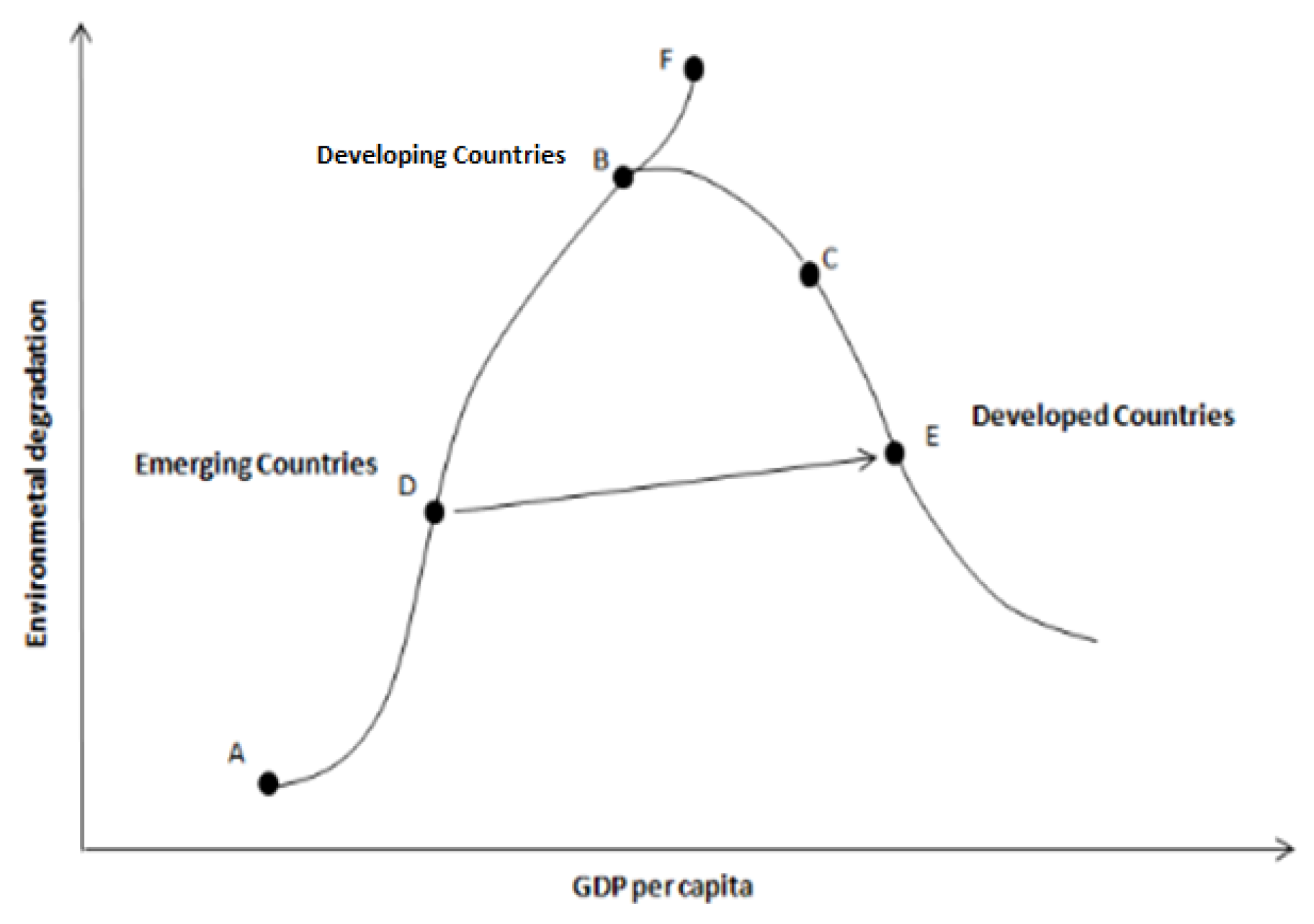
In
Figure 1
, point B shows the
target economic growth of developing countries that can proceed to point C
through sustainable development policies and clean technologies. The pathway
from point B to F generates more pollutants than financial growth, so it is
less likely to be followed. However, when emerging economies are given
financial support and environmental-friendly technologies, they are better
positioned to progress from point D to E, illustrating the tunnel effect. Thus,
we see a ‘grow now, clean later ’attitude in high-income countries, which
assumes that solutions to environmental problems can be developed at later
stages of economic growth. Therefore, in a dynamic economy, improved
technologies and policies that do not threaten economic growth are considered a
means to recover the environment (Gill et al., 2018).
According to the Global
Environment Outlook, the environment is changing faster, which calls for
governments to save the planet since ‘pollution and global warming are causing
millions of more deaths than conflicts’ are (United Nations, 2016). For
developed countries, this is a zero-sum game: On one hand, they seek more
incredible wealth, while on the other hand, they will have to spend large
amounts of capital on environmental recovery, primarily due to the higher costs
of pollution-abatement technologies. We thus evaluate the existence of the EKC
hypothesis by taking two primary variables: CO2 emissions and per
capita GDP. Based on the above discussion, the primary purpose of this study is
to examine the countries whose economic status changed from high-income to
previously high-income countries such as (Equatorial Guinea), a new country
entered in the high-income status (Argentina), and stable high-income (South
Korea). Equatorial Guinea is a Sub-Saharan country that changed its status to a
high-income country (2007–2014) ‘after the discovery of huge oil reserves in
1996, with 1.7 billion bbl. and average daily oil production of 0.3 million
BOPD as of December 2013’ (BP, 2014) (Echendu et al., 2015). Cronin et al.
(2015) report that Equatorial Guinea underwent rapid economic growth due to its
oil exports, accounting for 90% of its revenues.
Argentina, the eighth-largest
country globally, defaulted seven times between 1825 and 2001’ (López &
Nahón, 2017). However, it ultimately changed its status to a high-income
country, becoming the third-largest Latin American economy. It is now a member
of the G20 due to its rich reserves of natural resources, export-based
agricultural zones, well-diversified industrial sector, high-technology sector,
literate population, and high Human Development Index rating.
Figure 2
illustrates the real GDP per capita of all three sample countries.
South Korea’s GDP is continuously rising, while Equatorial Guinea experienced a
boom at the end of the nineteenth century, followed by a fall after a decade.
Argentina’s growth traces a zig-zag pattern over the The third sample country
is South Korea. As per the International Monetary Fund, it is a highly
developed country that holds the rank of the world’s 11th largest economy by
nominal GDP and is one of the stable members of the world’s more prosperous
societies. South Korea is also a member of the G20. It moved from the
seventh-largest CO2 emitter to the twelfth largest in 2018 (World
Resource Institute). The governments’ strategic measures to promote ‘low
carbon-green growth’ under the National Green Growth Strategy (2009–2050) are
mainly responsible for this reduction in emissions (Zhang and Choi, 2013).
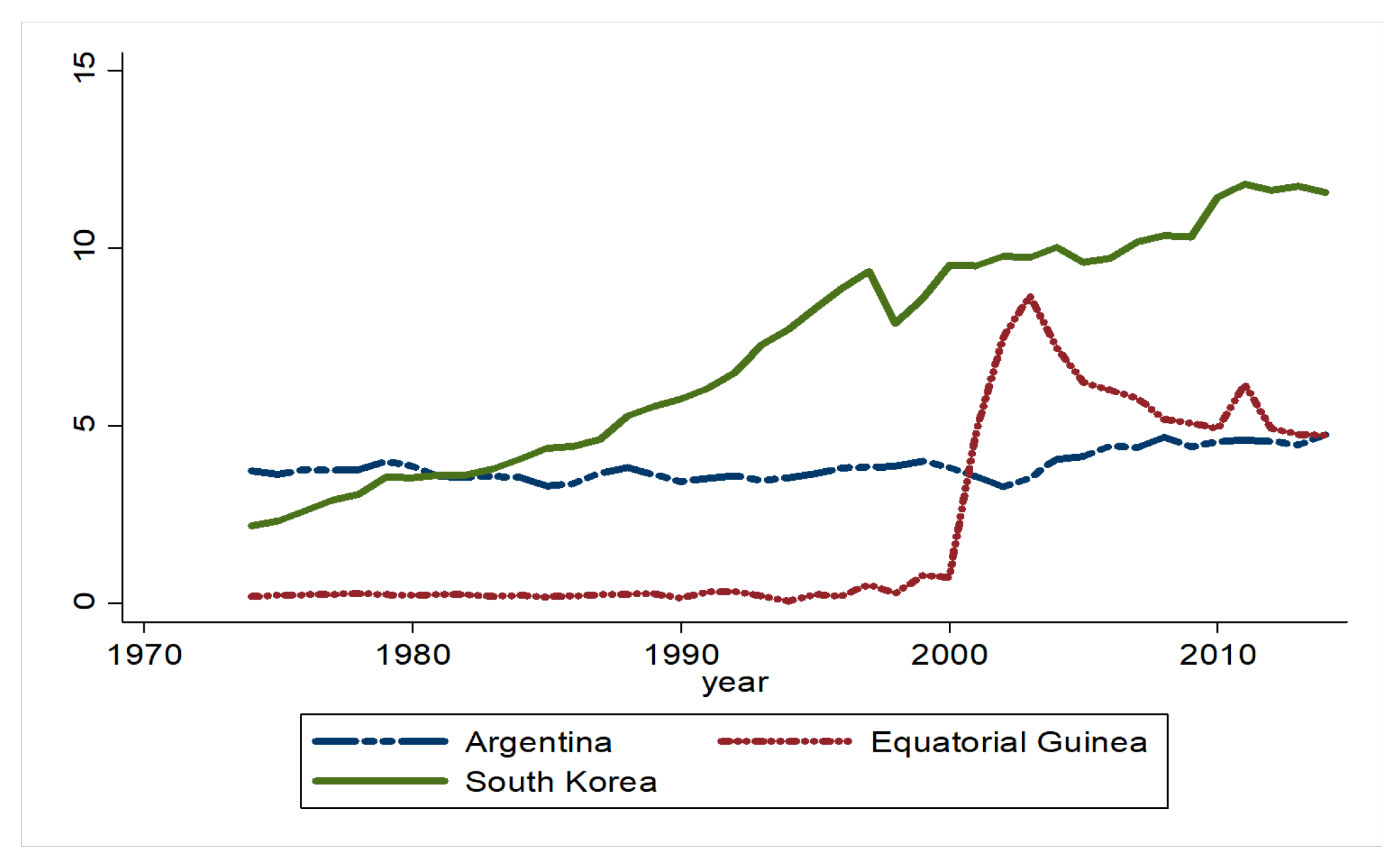
chosen period. The CO2
emissions of these countries also trace a similar pattern compared with
economic growth (
Figure 3
): South Korea has higher emissions, the emissions of Equatorial
Guinea peak when the country reaches higher per capita income, while Argentina
once again follows a meandering pattern. Recent years have shown that economic
study and policymaking cannot ignore the reality of the global climate crisis
when assessing the benefits of any given analytical tool or policy strategy. We
are now seeing widespread ecological calamities due to the failure to establish
a viable global climate stabilization program. Due to companies' substantial
involvement in climate change, attempts to stabilize the environment must be
seen as industrial rather than macroeconomic policy. The primary objective of
the climate stabilization endeavor is to significantly expand the renewable
energy industry while simultaneously shutting down the global fossil fuel
business
(Pollin, 2021) .
Previous studies only analyzed
the nexus between income and pollution. None of the studies have investigated
how the change in the income status from high to low and vice versa has
impacted their environmental health. To our knowledge, despite the importance
of evaluating the level of CO2 emissions in comparison with
increasing levels of income, the literature comprises no empirical studies on
individual high-income countries, especially those countries which transformed
their economic status, as in this study. Thus, we critically appraise the rise
in income against environmental pollutants for three developed countries from
1974 to 2020. Besides testing the EKC hypothesis, we also check for
co-integration and a causal relationship between GDP growth and CO2 emissions.
Figure 2.
GDP per Capita.
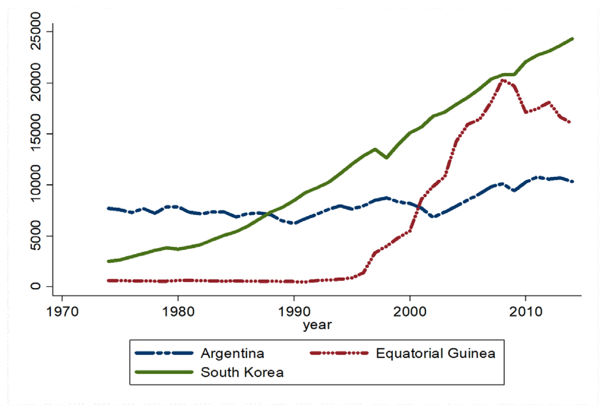
Figure 3.
CO2 Emissions per Capita.
The remaining paper is organized
as follows:
Section 2
presents the literature survey.
Section 3
encloses the data
model and methodology.
Section 4
reports the empirical results. Finally, section 5 presents the
conclusion.
2. Literature Review
Energy consumption promotes
economic growth. There is a growing body of literature on the causal
relationship between economic growth and environmental deregulation. This phenomenon was first coined by Kuznets (1955), known as the Kuznets
curve. Furthermore, Berthier et al., (2010) indicated an inverted
U-shaped relationship between economic growth and income inequality. Later,
Gross man and Krueger 1991 found a similar relationship between environmental
conditions, economic growth, and EKC. It hypothesizes an inverted U-shaped
relationship between real income and environmental pollution. That is, ‘as per
capita income increases, environmental pollution also increases at first and
then starts declining at a turning point.’ Numerous scholars and institutes
have endorsed the EKC model to protect the loss of environmental health from
economic activities. The World Development Report (IBRD, 1992) of the World
Bank, backed by Shafik (1994), states that environmental quality is an
essential element of sustainable development. Thus, numerous studies have
modeled the relationship between economic growth and CO2 emissions,
one of the highest observed pollutants in environmental economics studies.
Several scholars have tested the
EKC hypothesis against multiple indicators of environmental deterioration. For
example, Mather et al. (1999), Koirala and Mysami (2015), Bulte and van Soest
(2001), Stern et al. (1996), Ehrhardt-Martinez et al. (2002), Koop and Tole
(1999), and Panayotou (1994) attribute the extensive
deforestation to environmental deregulation. Moreover, sulfur dioxide (SO2)
was found to be another cause, according to the empirical findings (Brajer et
al., 2008; Arouri et al., 2012; Kaufmann et al., 1998; Selden and Song, 1994;
Zhoumu et al., 2015) and after all municipal waste was analyzed by (Bhattarai
and Hammig, 2001; Khajuria et al., 2011; Mazzanti et al.,2006; 2009).
Most of the literature on the EKC
hypothesis focuses on developed and developing countries (Cetin, 2018; Iwata
et al., 2012; Liu et al., 2019; Perman and Stern, 2003; Sinha Babu and Datta,
2013). These studies neglect the policy implications of economic growth and
environmental deregulation (Ang, 2008). This limitation necessitates studies
that can help in sustainable development policies at the country level. As
Stern et al. (1996b) believe, ‘A more fruitful approach for analyzing the
relationship between economic growth and environmental impact would be
examining the historical experience of individual countries, using econometric
and qualitative historical analyses. A comprehensive study by Zhang et
al.(2021) indicated a varied influence on nations with a high GDP per capita.
Additionally, the study
demonstrates that public investment in human capital and further developing
green energy technologies fosters a sustainable green economy via
labor-intensive and technology-oriented industrial activities, with varying
consequences in various nations (Sohu et al., 2023).
Taghizadeh-Hesary et al. (2021) examined the amount of investment in green
projects, particularly in the green power sector, is constrained by factors
such as insufficient long-term financing, various hazards, and a poor rate of
return on investment. Iqbal et al. (2021) propose many policy implications or
remedies to assist governments, institutions, companies, and the general people
in reducing environmental pollution through green financing. However, in a
recent study, Taghizadeh-Hesary et al. (2021) found that the COVID-19 epidemic
and worldwide recessions have resulted in a global decline in investments in
green initiatives jeopardizing the attainment of climate-related targets. As a
result, the post-COVID-19 world must transition to a green financial system by
introducing new financial instruments. Green bonds—a loan instrument aimed at
financing sustainable infrastructure projects—are gaining prominence in this
area.
However, scholars have tested the
EKC hypothesis by using time-series data for individual countries (Chen, 2012;
Friedl and Getzner, 2003; Halkos and Tzeremes, 2011; Hussain et al., 2012;
Lindmark, 2002; Mohapatra and Giri, 2009; Roca et al., 2001; Vollebergh et al.,
2011). Decade’s worth of studies have evaluated EKC hypothesis testing using
distinct methodologies, and this stream of research has resulted in a rich
array of perspectives. For instance, computational techniques have shifted the
research focus from simple EKC testing using static ordinary least squares
(OLS) models to a combination of dynamic models. EKC indicators include GDP to
foreign direct investments, population density, agriculture base, electricity
consumption, and trade-related proxies.
Consequently, the findings in the
literature reflect immense heterogeneity, from no existence of EKC to inverted
a U- or N-shaped curve (Yongsung et al., 2011). Further, Egli (2005) tested the
EKC hypothesis with co-integration and the causal
relationship, distinguishing the short- and long-run effects of financial
growth on the concentration of environment-deteriorating elements in the
atmosphere. Considering the vast literature on the EKC that uses multiple
indicators, large datasets, and different econometric methodologies, we
significantly contribute to this discipline by analyzing the existence of the
EKC hypothesis based on economic growth and pollutant emissions in the three
developed countries. In other words, when these countries’ financial status
changes or remains the same, what happens to their CO2 emissions? A
comprehensive study by Li et al. (2020) and Akbar et
al. (2023) investigate the effect of environmental
diplomacy on a country's carbon emissions. To examine whether environmental
accords resulted in reductions in CO2 emissions. The study concludes that both
developed and developing nations do not adhere to treaty standards in the long
term since CO2 emissions grow as the number of treaties increases. In general,
findings suggest that environmental accords are likely to waste international
diplomacy that does little to address climate change. One more study by Zakari
and Toplak (2021) emphasized the need for policymakers to consider non-economic
and non-technological elements, such as ethics, to achieve ecologically and
economically sustainable development. Furthermore, countries enact
environmental legislation to safeguard the environment. According to Zakari et
al. (2021), environmental accords have a considerable beneficial impact on the
environment in resource-poor nations that may help them achieve sustainable
development growth by 2030.

Table 1.
Descriptive Statistics.
| Argentina | Equatorial Guinea | South Korea | |||||||
|---|---|---|---|---|---|---|---|---|---|
| CO2 | GDP | GDP2 | CO2 | GDP | GDP2 | CO2 | GDP | GDP2 | |
| Mean | 1.34 | 8.98 | 13.15 | -0.29 | 7.71 | 17.39 | 1.84 | 9.16 | 16.93 |
| Median | 1.32 | 8.94 | 13.35 | -1.25 | 6.64 | 17.77 | 2.04 | 9.31 | 17.62 |
| Maximum | 1.55 | 9.28 | 15.79 | 2.15 | 9.92 | 18.86 | 2.46 | 10.09 | 18.86 |
| Minimum | 1.19 | 8.73 | 9.09 | -2.69 | 6.18 | 13.21 | 0.78 | 7.82 | 10.66 |
| Std. Dev. | 0.10 | 0.14 | 1.74 | 1.53 | 1.52 | 1.06 | 0.51 | 0.71 | 1.78 |
| Skewness | 0.62 | 0.68 | -0.46 | 0.50 | 0.37 | -1.78 | -0.52 | -0.36 | -1.57 |
| Kurtosis | 2.27 | 2.52 | 2.52 | 1.51 | 1.31 | 7.07 | 1.93 | 1.77 | 5.31 |
| Jarque–Bera | 3.56 | 3.56 | 1.88 | 5.50 | 5.81 | 50.05 | 3.79 | 3.48 | 26.12 |
| Probability | 0.16 | 0.16 | 0.39 | 0.06 | 0.05 | 0.00 | 0.14 | 0.17 | 0.00 |
3. Data and Methodology
3.1. Data
We
use annual data on per capita CO2emissions and per capita real GDP
measured in metric tons and constant 2010 US dollars, respectively. Data on
Argentina, Equatorial Guinea, and South Korea data are collected from the World
Development Indicator (2021) of the World Bank, covering 1974 to 2020. The
countries are selected based on data availability and current, previous, and
continued high-income countries.
Carbon
emissions are taken as the dependent variable to capture the nonlinear
relationship between income and CO2 emissions, with two independent
variables, GDP and EKC term: the square of GDP, to predict the short-run and
long-run elasticities.
Table 1
reports the descriptive statistics of the sample time series in a
natural logarithm.
3.2. Model and Methodology
To verify the presence of the
environmental Kuznets curve in the sample countries, we follow three steps.
First, we investigate the long-run relationship among the variables by
employing the autoregressive distributed lag (ARDL) bounds test of co-integration. Second, we use the Granger causality test to test the
causal relationship among the variables' time series. Then, the robustness
analysis is conducted using fully modified ordinary least squares (FMOLS),
dynamic ordinary least squares (DOLS), and canonical co-integrating regression (CCR). Generally, the EKC hypothesis is
specified using the following equation:”
Where the dependent variable
is the environmental factor,
is the income, and
denotes the variables responsible
for environmental deregulation. Our objective is to assess the causal
relationship between economic growth and environmental stability for the sample
of current, previous, and continued high-income countries. Instead of taking
additional variables, we take only income and CO2 emissions in our model. The
following equation corresponds to the logarithmic form of the model:
Here, each variable is in
form,
where
is the time,
is the CO2 emissions at
the per-capita level,
is the per capita real GDP, and
is the standard error term. To
validate the existence of the EKC hypothesis and confirm its significance, the
signs of the two coefficients
and
should be positive and negative,
respectively. It indicates an inverted U-shaped relationship between real
income and CO2 emissions.
There are many methods for
conducting the co-integration analysis, including the residual-based approach
by Engle and Granger (1987), the maximum likelihood approach by Johansen and
Juselius (1990), and the fully modified OLS procedure by, and the ARDL by (Pesaran et al., 2001). We use
the ARDL bounds testing approach because it has several advantages over
conventional methods. For instance, the method has better reliability for small
samples, has no endogeneity, and estimates long-and short-run coefficients to
simultaneously capture the independent variables' effect on the dependent
variable. Further, the method allows openness for integration order
irrespective of whether the variables are stationary at
I (0) or I(1) or a mixture of both. To capture the co-integration
relationship between real income growth and CO2 emissions through
the unrestricted error correction regressions, we estimate as follows:
In equation (2), is the drift element and is the error term. Further, , and are the error correction dynamics,
whereas, , and The long-run association and the
same pattern are applied to equations (3) and (4). In equation (2), following
the first step of the ARDL approach, we test the presence of the long-run co-integrating relationship using the null hypothesis—= 0—against the alternative
hypothesis ≠ 0—examined through the F
statistics. We apply the same process to equations (3) and (4).
“Next,
we determine the long-run co-integrating relationship
among the variables by comparing the calculated F statistics with two
sets of critical values found in the literature (Pesaran
et al., 2001b). The first set comprises the lower
critical bound (LCB) values for I(0) variables,
while the second set holds the upper critical bound values (UCB) for I(1)
variables. The null hypothesis of ‘no co-integration’
will be rejected if the calculated F statistics value is higher than the
UCB value, but the hypothesis cannot be rejected if the calculated F
statistics value is smaller than the LCB value. The value between the two
limits, UCB and LCB, will be inconclusive when the long-run association among
the variable series is confirmed with a negative and significant value of the
error correction term (ECT). Moreover, to run the ARDL model, the order of lags
is based on the Schwartz Bayesian criteria (SBC) and
Akaike’s information criteria (AIC), which select the smallest possible and
maximum relevant lag lengths, respectively. Once the existence of a long-run
relationship has been confirmed, we estimate the error correction model (ECM)
and Karagozoglu and Lindell (2000) as follows:”
The
equations (5) to (7) indicate the
speed of adjustment, that is, the time taken to restore the long-run
equilibrium. Diagnostic tests such as functional form, serial correlation,
normality, and heteroscedasticity tests are conducted to ensure the model's
fitness. Further, as per (Pesaran et al., 2001b), the long- and short-run stability coefficients are checked using
the cumulative sum and cumulative sum square tests. These tests
confirm the model’s stability if the test statistics value lies within the plot
of two straight lines representing critical bounds at the 5% significance
level. Note that the ARDL method only confirms the presence or non-existence of
co-integration among variables series, so we employ the
(Granger 1969) test to verify the existence and direction of causality. The
enlarged version of the Granger causality test with the ECM encompassing the
vector error correction model (VECM) and multivariate nth
order is formulated as follows:
Where
is the lag operator,
denotes the parameters of
estimation,
denotes the zero mean uncorrelated
random disturbance terms, and
is the lagged error term. The VECM
determines the direction of the
causality, while the
significance value of the lagged ECT,
,
verifies
the long-run causal relationship among the variable series. In addition, the
short-run Granger causal relationship can be detected through the significant F
statistics value of the lagged independent variables.
4. Empirical Results
4.1. Unit-Root Tests
Before the ARDL model, we employ
three-unit root tests—augmented Dickey-Fuller, Phillips–Person, and
Lee–Strazicich tests—to confirm the required I (0) or I(1)
integration order of variables series. Because of the
substantial likelihood, the sample data contain structural breaks, thus
avoiding the spurious results of traditional stationarity tests. The
Lee–Strazicich test is used if a structural break(s) occur(s) in the data,
where the augmented Dickey-Fuller (1979) and PHILLIPS- PERRON (1988) tests
would generate misleading and biased results (Phillips & Perron, 1988).
The existence of a single
structural break that further extends to two and five breaks was proposed by
Zivot and Andrews (1992), Lumsdaine and Papell (1997), and Kapetanios (2005),
respectively. However, these tests bear a linearity assumption limitation under
the null hypothesis.
Therefore, if there is a break
under the null hypothesis, we will observe size distortions that will lead us
to reject the null hypothesis as these results are erroneously estimated
breakpoints (ALTINAY, 2005). Lee and Strazicich (2004) developed their test to
overcome the assumption that breaks are accommodated under null and alternative
hypotheses.
Table 2
reports the empirical findings of the unit root tests, starting
with the augmented Dickey-Fuller and Phillips–Person tests, followed by the
Lee–Strazicich tests with single and double structural breaks. In structural
breaks in the time series, we find three series: CO2 emissions of
Argentina and South Korea and the GDP of Equatorial Guinea are stationary at
the first difference, while the remaining series are stationary at level.
Table 2.
Augmented Dickey–Fuller, Phillips–Person, and Lee and Strazicich (2004) with single and double structural breaks.
Table 2.
Augmented Dickey–Fuller, Phillips–Person, and Lee and Strazicich (2004) with single and double structural breaks.
|
Variable |
ADF test |
PP test |
Lee–Strazicich test (One Break) |
Lee–Strazicich test (Two Breaks) |
|||||||
|---|---|---|---|---|---|---|---|---|---|---|---|
| t-Statistic | I(•) | t-Statistic | I(•) | t-Statistic | TB1 | I(•) | t-Statistic | TB1 | TB2 | I(•) | |
| Argentina | |||||||||||
| CO2 | -4.80*** | I(1) | -9.32*** | I(1) | -4.57** (4) |
1993 | I(0) | -10.16*** (1) |
2007 | 2010 | I(1) |
| GDP | -5.26*** | I(1) | -5.17*** | I(1) | -6.32*** (7) |
1987 | I(0) | -6.23** (7) |
1989 | 2000 | I(0) |
| GDP2 | -6.56*** | I(1) | -13.37*** | I(1) | 5.90*** (1) |
1995 | I(0) | -7.71*** (1) |
1991 | 1995 | I(0) |
| Equatorial Guinea | |||||||||||
| CO2 | -7.78*** | I(1) | -7.65*** | I(1) | -5.34*** (7) |
1998 | I(0) | -6.21** (7) |
1991 | 1999 | I(0) |
| GDP | -3.50** | I(1) | -3.48** | I(1) | -5.76*** (7) |
1995 | I(0) | -10.16*** (1) |
2007 | 2010 | I(1) |
| GDP2 | -6.56*** | I(1) | -13.3*** | I(1) | -4.92*** (7) |
1994 | I(0) | -7.71*** (1) |
1991 | 1995 | I(0) |
| South Korea | |||||||||||
| CO2 | -6.51*** | I(1) | -6.62*** | I(1) | -4.84** (4) |
2001 | I(0) | -7.46*** (4) |
1996 | 2002 | I(1) |
| GDP | -4.56*** | I(1) | -5.80*** | I(1) | -6.37*** (7) |
1998 | I(0) | -5.84* (5) |
1991 | 2003 | I(0) |
| GDP2 | -6.39*** | I(1) | -6.42*** | I(1) | -4.25* (8) |
1997 | I(1) | -6.65** (7) |
1992 | 2004 | I(0) |
Notes. The numbers in parentheses are t statistics. *, **, and *** indicate statistical significance at the 10%, 5%, and 1% levels.
We find that every variable series of each country is non-stationary at the level under the former two tests; when transformed to the first difference, each series rejects the null hypothesis at the 1% significance level. On the other hand, Lee and Strazicich (2004) demonstrated a different integration order; except for South Korea’s GDP square, the remaining series of the three countries are stationary at the level for single the break hypothesis. Finally, for more robust testing, we find three series for two structural breaks in the time series: CO2 emissions of Argentina and South Korea and the GDP of Equatorial Guinea are stationary at the first difference, while the remaining series are stationary at level.
4.2. Cointegration
In the next step, we use the most widely used co-integration measure, ARDL bounds testing, developed (Pesaran et al., 2001b) to capture the long-run equilibrium among the variable series. Bounds testing is advantageous compared with other conventional co-integration techniques for three reasons. First, it can be applied to both a mixed I(0) or I(1) integration order. Second, it performs well with a small or finite sample size(Narayan, 2005). Third, it is a bias-free technique for long-run estimations (Harris and Sollis, 2003). The decision regarding co-integration is based on an F statistics comparison with the UC Band LCB values. The UCB considers all variables at I(1) integration order, while LCB takes level order I(0) for all variables (Pesaran et al., 2001). Therefore, a weaker UCB value than the computed F-statistics would validate co-integration among variables. Therefore, the decision is reserved when the F statistics value is below the LCB value. However, the decision on co-integration presence will be inconclusive if the computed value of the F statistics is less than the UCB value and more than the LCB value. In this case, the lagged ECT decides the long-term relationship. The results in Table 3 present the F statistics of three countries based on the null hypothesis—H0: 1= 2= 3=0—against the alternative hypothesis—H1: 1≠ 2 ≠ 3≠0, denoting CO2 emissions as the dependent variable, while the GDP and GDP square are the independent variables.
The F statistics values for Argentina, Equatorial Guinea, and South Korea are 9.225, 11.463, and 9.250, respectively, which are much higher than the UCB values to reject the null hypothesis at the 1% significance level. Such a rejection implies that the CO2 emissions, GDP, and GDP square series are mutually co-integrated in Argentina, Equatorial Guinea, and South Korea. After verifying co-integration in the time series, we conduct the causality test by deriving the marginal impact of GDP and GDP square on the CO2 emissions for the long-and short-run elasticities. That allows us to confirm the existence of the EKC for the sample countries.
As shown in Table 4, the per capita GDP positively and statistically significantly impacts CO2 emissions. Specifically, a 1% permanent increase in GDP raises CO2 emissions in the long run by 0.60% and 0.96% in Argentina and Equatorial Guinea, respectively. The same pattern continues for GDP square: A 1% increase in GDP square significantly boosts the CO2 emissions by 0.01% and 0.28% in that order for both countries. For South Korea, the significant positive and negative long-run elasticities are 0.67% and -0.02% for GDP and GDP square, respectively, which aligns with our expectations. That confirms the existence of EKC in South Korea. We now proceed to short-run results and diagnostic tests (Table 5). The short-run elasticities for each of the three countries are computed using the ECM from equations (5) to (7). The results show a positive and significant relationship between Argentina's economic growth and CO2 emissions.
Their coefficient of the GDP square is less than zero and insignificant; hence, the results do not support the EKC hypothesis in the short run. For Equatorial Guinea, we find a significant and positive relationship between GDP growth and CO2 emissions but a negative and significant coefficient of GDP square. That indicates the existence of the EKC in the short run at the 1% significance level. Finally, after validating an inverted U-shaped curve between GDP growth and CO2 emissions in the long run, we confirm the short-run existence of the EKC for South Korea for GDP and at a two-time lag of the GDP square.
The stability of the ECM coefficients and the long-run goodness of fit for the model are further confirmed with the cumulative sum and cumulative sum square. The two ECMs for the three countries are illustrated in Figure 4, Figure 5, Figure 6, Figure 7, Figure 8 and Figure 9: All remain within the critical bounds at the 5% significance level.
After yielding successful results on the cointegrated causal relationship between CO2emissions and economic growth, we employ the VECM Granger causality test to identify the direction of the relationship among the time series. Table 6 reports the results of the Granger causality test, indicating a significant long-run relationship for all three countries. However, Argentina shows a bidirectional long-run significant relationship between GDP and CO2 emissions.
In the short run, findings from Argentina reveal a unidirectional negative causal relationship that runs from GDP square to CO2 emissions. We observe several short-run Granger causalities for Equatorial Guinea; the results reveal a unidirectional positive and significant short-run relationship from GDP to CO2 emissions. The only bidirectional and significant relationship between GDP square and CO2 emissions exists at the 5% level. Finally, the results for South Korea indicate a unidirectional short-run negative causality from economic growth to CO2 emissions.
Table 7 reports the results of the FMOLS, DOLS, and CCR estimators to check the robustness of the model. The robustness of the long-run findings of the ARDL estimations for the three countries is fully validated. The results confirm the absence of the EKC in the long run for Argentina and Equatorial Guinea but a presence for South Korea.
5. Conclusions
We explored the EKC hypothesis's existence, including causal and long-run relationships between CO2 emissions and economic growth per capita for Argentina, Equatorial Guinea, and South Korea. The period covers 1974 to 2020, and we used the ARDL method proposed by (Pesaran et al. (2001a) and the FMOLS, DOLS, CCR, causality, and stability tests. We found that all three countries exhibit a robust long-run relationship between CO2 emissions and per capita GDP. An inverted U-shaped curve exists only in the short run for Equatorial Guinea and South Korea. In the long run, only South Korea exhibits the EKC. The FMOLS, DOLS, and CCR estimations confirm the long-run findings of the ARDL approach, which confirms the robustness of the results. The VECM Granger causality test checked the variables' linkage and direction of causality. It specified a significant long-run relationship from GDP to CO2 emission for each country; except for Argentina, the remaining two countries exhibit a bidirectional long-run significant relationship. This result proves that the decoupling of the two variables is unlikely under the economic policy structure of the sample countries.
In the short run, Argentina has a similar unidirectional negative relationship that runs from GDP square to CO2 emissions, whereas South Korea exhibits a unidirectional negative causality from GDP to CO2 emissions. Equatorial Guinea exhibits more causal associations following the long-run path: a significant and negative unidirectional positive relationship from GDP to CO2 emissions and the only bidirectional and significant negative relationship between GDP square and CO2 emissions.
Conclusively, in the short run, Argentina’s GDP square has a negative impact on CO2 emissions. For South Korea, economic growth has a negative impact on CO2 emissions. Finally, for Equatorial Guinea, the GDP has only a positive impact, while the GDP square has a positive and negative impact on CO2 emissions. It implies that in the short run, after the turning point on the EKC curve, an increase in the GDP causes a decline in CO2 emissions in Argentina. In the long run, the unidirectional causality from GDP to CO2 emissions indicates that the Argentinian government must invest more in pollution abatement policies to encourage sustainable development. Pollution reduction strategies such as emissions tax, carbon credit policy, enhanced use of clean energy technologies, and energy efficiency schemes will not harm the long-term economic growth of this newly high-income country but cement its economic status along with better environmental conditions.
In Equatorial Guinea, a former high-income country that once experienced the oil boom, a short-run, bidirectional, positive, and negative relationship runs from GDP square to CO2 emissions. Thus, the rise and fall in the GDP square align with the economic growth. That is, the EKC hypothesis in the short run is confirmed. Thus, Equatorial Guinea must employ environmentally friendly measures and stringent environmental laws without adversely affecting GDP growth. In South Korea, an increase in GDP does not increase the pollution level in the short run, which is a rare case that might be attributed to the country’s ‘low carbon green growth’ policy(see section 1) and five-year plan for green growth (2009–2013). These short-run causality results for South Korea are in line with Sonnenschein and Mundaca (2016), who revealed a short-term (2008–2012) enhancing effect of GDP per capita on CO2 emissions with lower emissions. However, the 1971–2012 period is evidence of worsening CO2 intensity during the early years of the Green Growth Strategy. Therefore, South Korea still requires a more robust low-carbon growth policy that matches its economic growth. It must discard fossil fuels subsidies and increase energy efficiency rather than offer ‘green growth engines.’ In addition, it must implement pricing reforms, carbon energy taxes, and a strict regulatory system. Without good sustainable development policies, stable financial growth in South Korea is impossible without environmental deterioration.
Future researchers may broaden this study to more high-income countries by using large and improved datasets. That would allow an analysis of these countries before and after becoming high-income countries. It would also refine findings to understand long-term policy implications, thus ensuring continuous environmentally sustainable growth.
Funding
This research received no external funding.
Acknowledgments
Special credit to my father Mr. Ghulam Akbar Arbani, for being my lifelong motivation and for being a great source of learning.
Conflicts of Interest
The authors declare no conflict of interest.
References
- Akbar, .S., Bhutto, N.A. & Rajput, S.K.O. How do carbon emissions and eco taxation affect the equity market performance: an empirical evidence from 28 OECD economies. Environ Sci Pollut Res (2023). [CrossRef]
- ALTINAY, G. (2005). STRUCTURAL BREAKS IN LONG-TERM TURKISH MACROECONOMIC DATA,1923-2003. Applied Econometrics and International Development., 5(4).
- Ang, J. B. (2008). Economic development, pollutant emissions and energy consumption in Malaysia. Journal of Policy Modeling, 30(2). [CrossRef]
- Arouri, M. E. H., Youssef, A. Ben, M’Henni, H., & Rault, C. (2012). Empirical analysis of the EKC hypothesis for sulfur dioxide emissions in selected middle east and north African countries. Journal of Energy and Development, 37(2), 207–226.
- Baldo, M. A., O’Brien, D. F., You, Y., Shoustikov, A., Sibley, S., Thompson, M. E., & Forrest, S. R. (1998). Highly efficient phosphorescent emission from organic electroluminescent devices. Nature, 395(6698), 151–154. [CrossRef]
- Beckerman, W. (1992). Economic growth and the environment: Whose growth? whose environment? World Development, 20(4). [CrossRef]
- Berthier, E., Schiefer, E., Clarke, G. K. C., Menounos, B., & Rémy, F. (2010). Contribution of Alaskan glaciers to sea-level rise derived from satellite imagery. Nature Geoscience, 3(2), 92–95. [CrossRef]
- Bhattarai, M., & Hammig, M. (2001). Institutions and the environmental Kuznets Curve for deforestation: A crosscountry analysis for Latin America, Africa and Asia. World Development, 29(6), 995–1010. [CrossRef]
- Brajer, V., Mead, R. W., & Xiao, F. (2008). Health benefits of tunneling through the Chinese environmental Kuznets curve (EKC). Ecological Economics, 66(4), 674–686. [CrossRef]
- Bulte, E. H., & van Soest, D. P. (2001). Environmental degradation in developing countries: households and the (reverse) Environmental Kuznets Curve. Journal of Development Economics, 65(1). [CrossRef]
- Cetin, M. A. (2018). Investigating the environmental Kuznets Curve and the role of green energy: Emerging and developed markets. International Journal of Green Energy, 15(1). [CrossRef]
- Chen, W. J. (2012). The relationships of carbon dioxide emissions and income in a newly industrialized economy. Applied Economics, 44(13), 1621–1630. [CrossRef]
- Cronin, D. T., Woloszynek, S., Morra, W. A., Honarvar, S., Linder, J. M., Gonder, M. K., O’Connor, M. P., & Hearn, G. W. (2015). Long-Term Urban Market Dynamics Reveal Increased Bushmeat Carcass Volume despite Economic Growth and Proactive Environmental Legislation on Bioko Island, Equatorial Guinea. PLOS ONE, 10(7). [CrossRef]
- Dasgupta, S., Laplante, B., Wang, H., & Wheeler, D. (2002). Confronting the environmental Kuznets curve. In Journal of Economic Perspectives (Vol. 16, Issue 1, pp. 147–168). [CrossRef]
- Dickey, D. A., & Fuller, W. A. (1979). Distribution of the Estimators for Autoregressive Time Series With a Unit Root. Journal of the American Statistical Association, 74(366). [CrossRef]
- Dinda, S. (2004). Environmental Kuznets Curve hypothesis: A survey. Ecological Economics, 49(4), 431–455. [CrossRef]
- Echendu, J. C., Iledare, O. O., & Onwuka, E. I. (2015). Comparative Economic-Performance Analysis of Production-Sharing Contracts in Angola, Equatorial Guinea, Gabon, and Nigeria. SPE Economics & Management, 7(04). [CrossRef]
- Egli, H. (2005). Are Cross-Country Studies of the Environmental Kuznets Curve Misleading? New Evidence from Time Series Data for Germany. SSRN Electronic Journal. [CrossRef]
- Ehrhardt-Martinez, K., Crenshaw, E. M., & Jenkins, J. C. (2002). Deforestation and the Environmental Kuznets Curve: A Cross-National Investigation of Intervening Mechanisms. Social Science Quarterly, 83(1). [CrossRef]
- Engle, R. F., & Granger, C. W. J. (1987). Co-Integration and Error Correction: Representation, Estimation, and Testing. Econometrica, 55(2). [CrossRef]
- Friedl, B., & Getzner, M. (2003). Determinants of CO2 emissions in a small open economy. In Ecological Economics (Vol. 45, Issue 1, pp. 133–148). [CrossRef]
- Granger, C. W. J. (1969). Investigating Causal Relations by Econometric Models and Cross-spectral Methods. Econometrica, 37(3). [CrossRef]
- Halkos, G. E., & Tzeremes, N. G. (2011). Growth and environmental pollution: Empirical evidence from China. Journal of Chinese Economics and Trade Studies, 4(3), 144–157. [CrossRef]
- Houghton, J. (2005). Global warming. Reports on Progress in Physics, 68(6), 1343–1403. [CrossRef]
- Hussain, M., Javaid, M. I., & Drake, P. R. (2012). An econometric study of carbon dioxide (CO2) emissions, energy consumption, and economic growth of Pakistan. International Journal of Energy Sector Management, 6(4), 518–533. [CrossRef]
- Iqbal, S., Taghizadeh-Hesary, F., Mohsin, M., & Iqbal, W. (2021). Assessing the Role of the green finance index in environmental pollution reduction. Estudios de Economia Aplicada, 39(3). [CrossRef]
- Iwata, H., Okada, K., & Samreth, S. (2012). Empirical study on the determinants of CO2 emissions: Evidence from OECD countries. Applied Economics, 44(27), 3513–3519. [CrossRef]
- Johansen, S., & Juselius, K. (1990). Maximum Likelihood Estimation and Inference on Cointegration — With Applications To the Demand for Money. Oxford Bulletin of Economics and Statistics, 52(2), 169–210. [CrossRef]
- Johnson, D. L., Ambrose, S. H., Bassett, T. J., Bowen, M. L., Crummey, D. E., Isaacson, J. S., Johnson, D. N., Lamb, P., Saul, M., & Winter-Nelson, A. E. (1997). Meanings of Environmental Terms. Journal of Environmental Quality, 26(3), 581–589. [CrossRef]
- Junsoo Lee and Mark Strazicich. (2004). Minimum LM Unit Root Test with One Structural Break.
- Kapetanios, G. (2005). Unit-root testing against the alternative hypothesis of up to m structural breaks. Journal of Time Series Analysis, 26(1). [CrossRef]
- Karagozoglu, N., & Lindell, M. (2000). Environmental Management: Testing the Win-Win Model. Journal of Environmental Planning and Management, 43(6). [CrossRef]
- Kaufmann, R. K., Davidsdottir, B., Garnham, S., & Pauly, P. (1998). The determinants of atmospheric SO2 concentrations: Reconsidering the environmental Kuznets curve. Ecological Economics, 25(2), 209–220. [CrossRef]
- Khajuria, A., Matsui, T., & Machimura, T. (2011). Economic Growth Decoupling Municipal Solid Waste Loads in Terms of Environmental Kuznets Curve: Symptom of the Decoupling in India. Journal of Sustainable Development, 4(3). [CrossRef]
- Koirala, B. S., & Mysami, R. C. (2015). Investigating the effect of forest per capita on explaining the EKC hypothesis for CO 2 in the US . Journal of Environmental Economics and Policy, 4(3), 304–314. [CrossRef]
- Kong, Y., & Khan, R. (2019). To examine environmental pollution by economic growth and their impact in an environmental Kuznets curve (EKC) among developed and developing countries. PLOS ONE, 14(3). [CrossRef]
- Koop, G., & Tole, L. (1999). Is there an environmental Kuznets curve for deforestation? Journal of Development Economics, 58(1), 231–244. [CrossRef]
- Kuznets, S. (1955). The American Economic Review VOLUME XLV MARCH, 1955 NUMBER ONE ECONOMIC GROWTH AND INCOME INEQUALITY*. Amrican Economic Association, 45(1), 1–28. Available online: https://edisciplinas.usp.br/pluginfile.php/306155/mod_resource/content/1/Kusnetz %281955%29 Economic Growth and income inequality.pdf.
- Li, G., Zakari, A., & Tawiah, V. (2020). Does environmental diplomacy reduce CO2 emissions? A panel group means analysis. Science of the Total Environment, 722. [CrossRef]
- Lindmark, M. (2002). An EKC-pattern in historical perspective: Carbon dioxide emissions, technology, fuel prices and growth in sweden 1870-1997. Ecological Economics, 42(1–2), 333–347. [CrossRef]
- Liu, H., Kim, H., & Choe, J. (2019). Export diversification, CO2 emissions and EKC: panel data analysis of 125 countries. Asia-Pacific Journal of Regional Science, 3(2). [CrossRef]
- López, P. J., & Nahón, C. (2017). The Growth of Debt and the Debt of Growth: Lessons from the Case of Argentina. Journal of Law and Society, 44(1). [CrossRef]
- Lumsdaine, R. L., & Papell, D. H. (1997). Multiple Trend Breaks and the Unit-Root Hypothesis. Review of Economics and Statistics, 79(2). [CrossRef]
- Mather, A. S., Needle, C. L., & Fairbairn, J. (1999). Environmental kuznets curves and forest trends. Geography, 84(362), 55–65.
- Mazzanti, M., Montini, A., & Zoboli, R. (2006). Municipal Waste Production, Economic Drivers, and “New” Waste Policies: EKC Evidence from Italian Regional and Provincial Panel Data. SSRN Electronic Journal. [CrossRef]
- Mazzanti, M., & Zoboli, R. (2009). Municipal Waste Kuznets curves: Evidence on socio-economic drivers and policy effectiveness from the EU. Environmental and Resource Economics, 44(2), 203–230. [CrossRef]
- Mohapatra, G., & Giri, A. K. (2009). Economic development and environmental quality: an econometric study in India. Management of Environmental Quality: An International Journal, 20(2). [CrossRef]
- Narayan, P. K. (2005). The saving and investment nexus for China: evidence from cointegration tests. Applied Economics, 37(17). [CrossRef]
- Panayotou, T. (1994). Empirical tests and policy analysis of environmental degradation at different stages of economic development. Pacific and Asian Journal of Energy, 4(1), 23–42.
- Perman, R., & Stern, D. I. (2003). Evidence from panel unit root and cointegration tests that the Environmental Kuznets Curve does not exist. Australian Journal of Agricultural and Resource Economics, 47(3). [CrossRef]
- Pesaran, M. H., Shin, Y., & Smith, R. J. (2001a). Bounds testing approaches to the analysis of level relationships. Journal of Applied Econometrics, 16(3), 289–326. [CrossRef]
- Pesaran, M. H., Shin, Y., & Smith, R. J. (2001b). Bounds testing approaches to the analysis of level relationships. Journal of Applied Econometrics, 16(3). [CrossRef]
- Phillips, P. C. B., & Perron, P. (1988). Testing for a unit root in time series regression. Biometrika, 75(2), 335–346. [CrossRef]
- PHILLIPS, P. C. B., & PERRON, P. (1988). Testing for a unit root in time series regression. Biometrika, 75(2). [CrossRef]
- Pollin, R. (2021). The industrial policy requirements for a global climate stabilization project. International Review of Applied Economics, 35(3–4). [CrossRef]
- Rashid Gill, A., Viswanathan, K. K., & Hassan, S. (2018). The Environmental Kuznets Curve (EKC) and the environmental problem of the day. Renewable and Sustainable Energy Reviews, 81. [CrossRef]
- Roca, J., Padilla, E., Farré, M., & Galletto, V. (2001). Economic growth and atmospheric pollution in Spain: discussing the environmental Kuznets curve hypothesis. Ecological Economics, 39(1). [CrossRef]
- Selden, T. M., & Song, D. (1994). Environmental quality and development: Is there a kuznets curve for air pollution emissions? Journal of Environmental Economics and Management, 27(2), 147–162. [CrossRef]
- Shafik, N. (1994). Economic development and environmental quality: An econometric analysis. Oxford Economic Papers, 46, 757–773. [CrossRef]
- Sinha Babu, S., & Datta, S. K. (2013). The relevance of environmental Kuznets curve (EKC) in a framework of broad-based environmental degradation and modified measure of growth-a pooled data analysis. International Journal of Sustainable Development and World Ecology, 20(4), 309–316. [CrossRef]
- Sohu, J. M., Hongyun, T., Akbar, U. S., & Hussain, F. (2023). Digital Innovation, Digital Transformation, and Digital Platform Capability: Detrimental Impact of Big Data Analytics Capability on Innovation Performance. International Research Journal of Management and Social Sciences, 4(3), 265-281. [CrossRef]
- Sonnenschein, J., & Mundaca, L. (2016). Decarbonization under green growth strategies? The case of South Korea. Journal of Cleaner Production, 123. [CrossRef]
- Stern, D. I., Common, M. S., & Barbier, E. B. (1996a). Economic growth and environmental degradation: The environmental Kuznets curve and sustainable development. World Development, 24(7), 1151–1160. [CrossRef]
- Stern, D. I., Common, M. S., & Barbier, E. B. (1996b). Economic growth and environmental degradation: The environmental Kuznets curve and sustainable development. World Development, 24(7). [CrossRef]
- Taghizadeh-Hesary, F., Yoshino, N., Rasoulinezhad, E., & Rimaud, C. (2021). Power purchase agreements with incremental tariffs in local currency: An innovative green finance tool. Global Finance Journal, 50. [CrossRef]
- Thripp, R. (2019). A Ratio for the Relative Climate Change Impact of an Economic Activity. SSRN Electronic Journal, 36–38. [CrossRef]
- Vollebergh, H. R. J., Dijkgraaf, E., & Melenberg, B. (2011). Environmental Kuznets Curves for CO2: Heterogeneity versus Homogeneity. SSRN Electronic Journal. [CrossRef]
- Zakari, A., Adedoyin, F. F., Taghizadeh-Hesary, F., & Pazouki, A. (2021). Environmental treaties’ impact on the environment in resource-rich and non-resource-rich countries. Environmental Science and Pollution Research, 28(25). [CrossRef]
- Zakari, A., & Toplak, J. (2021). Investigation into the social behavioural effects on a country’s ecological footprint: Evidence from Central Europe. Technological Forecasting and Social Change, 170. [CrossRef]
- Zhang, D., Mohsin, M., Rasheed, A. K., Chang, Y., & Taghizadeh-Hesary, F. (2021). Public spending and green economic growth in BRI region: Mediating role of green finance. Energy Policy, 153. [CrossRef]
- Zhang, N., & Choi, Y. (2013). A comparative study of dynamic changes in CO2 emission performance of fossil fuel power plants in China and Korea. Energy Policy, 62. [CrossRef]
- Zhoumu, Y., Wenping, W., Yibo, Y., & Fen, F. (2015). An Empirical Study of Environmental Kuznets Curve in China. [CrossRef]
- Zivot, E., & Andrews, D. W. K. (1992). Further Evidence on the Great Crash, the Oil-Price Shock, and the Unit-Root Hypothesis. Journal of Business & Economic Statistics, 10(3). [CrossRef]
- 최은호, Yongsung CHO, & Heshmati, Almas. (2011). An Empirical Study of the Relationships between CO_2 Emissions, Economic Growth and Openness. Journal of Environmental Policy, 10(4), 3–37. [CrossRef]
Figure 4.
Argentina cumulative sum graph.
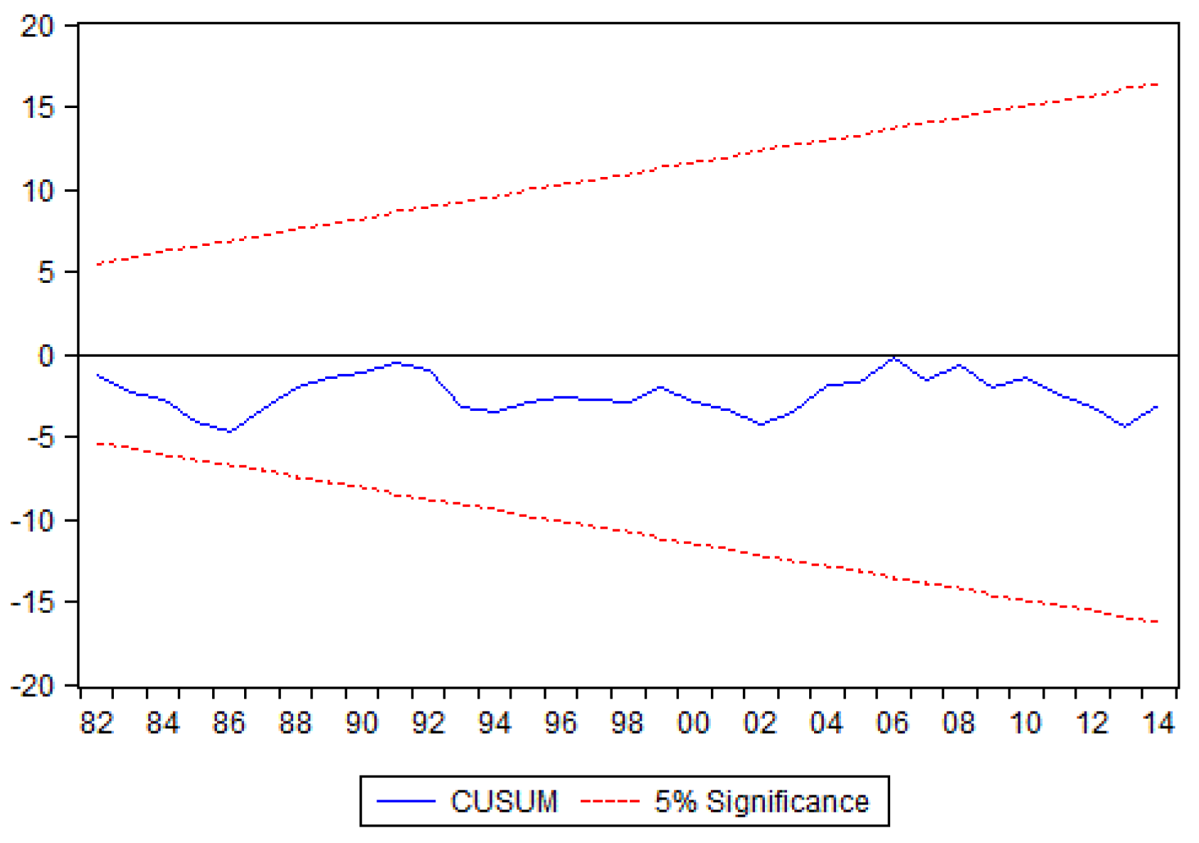
Figure 5.
Argentina cumulative sum square graph.
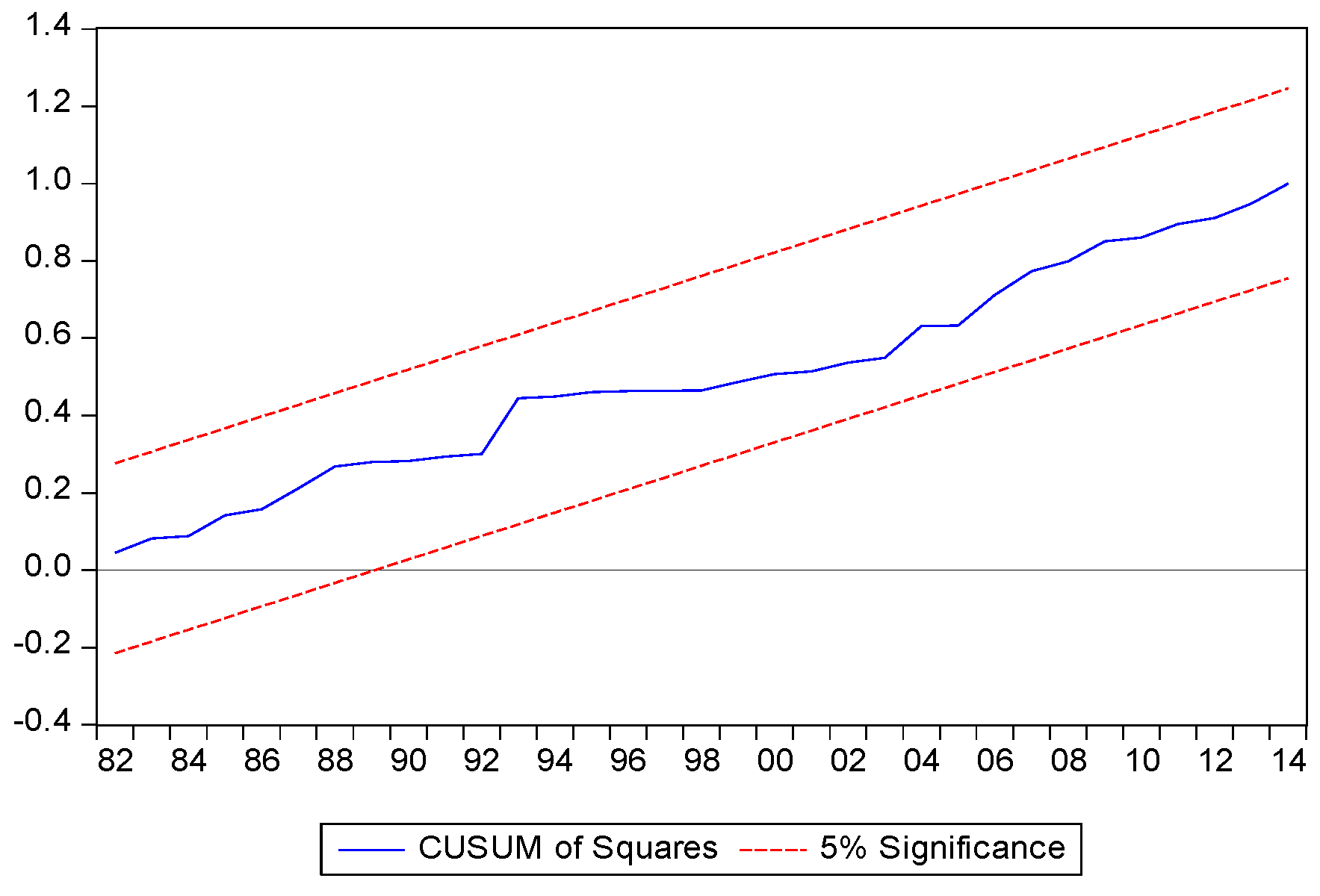
Figure 6.
Equatorial Guinea cumulative sum graph.
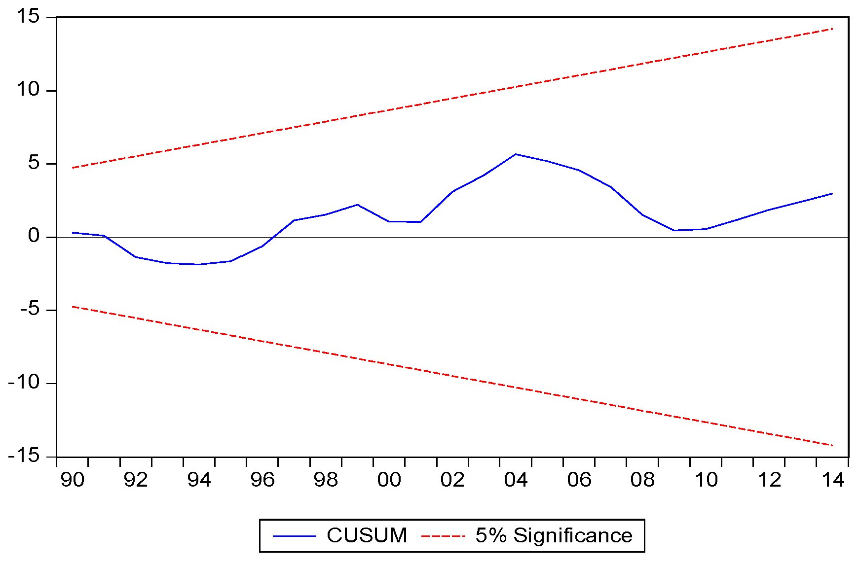
Figure 7.
Equatorial Guinea cumulative sum square graph.
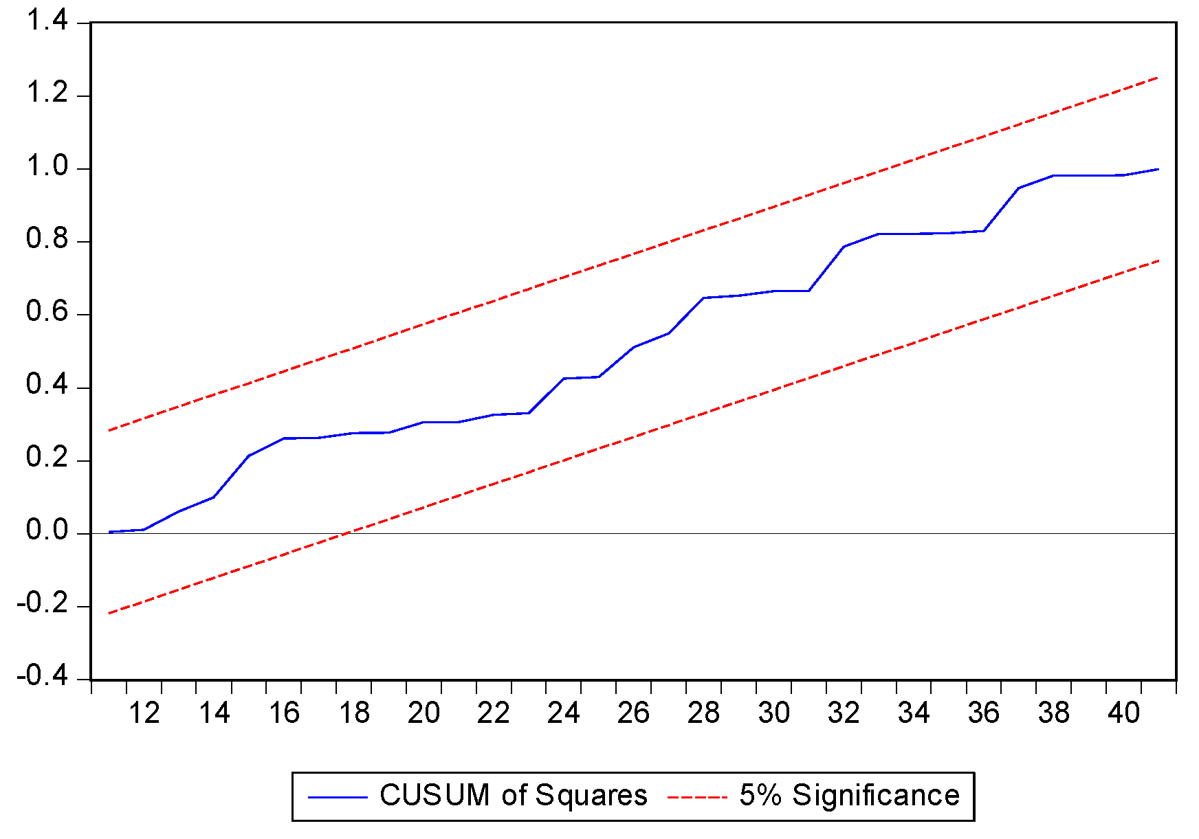
Figure 8.
South Korea cumulative sum graph.
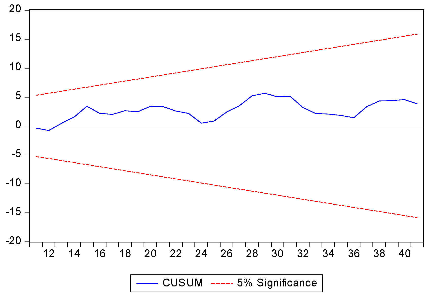
Figure 9.
South Korea cumulative sum square graph.
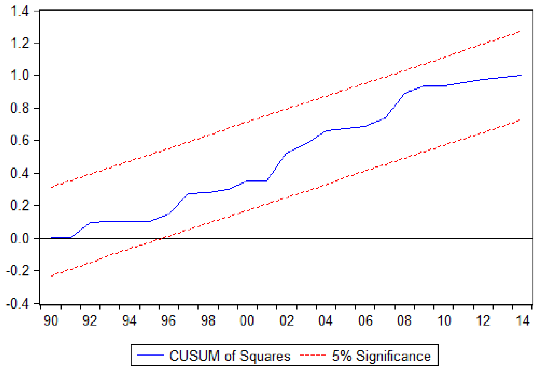
Table 3.
The Results of Co-integration.
| Country | Argentina | Equatorial Guinea | South Korea |
|---|---|---|---|
| F statistics | 9.225*** | 11.463*** | 9.250*** |
| Significance level | 1% | 5% | 10% |
| I (0) | 5.15 | 3.79 | 3.17 |
| I (1) | 6.36 | 4.85 | 4.14 |
Note. The numbers in parentheses are t statistics. *, **, and *** indicate statistical significance at the 10%, 5%, and 1% levels.
Table 4.
ARDL long run estimation results.
| New High Income | Old High Income | Stable High Income | |||||||
| Argentina | Equatorial Guinea | South Korea | |||||||
| ARDL (2,0,1) based on SBIC | ARDL (3,4,2) based on AIC | ARDL (1,0,3) based on SBIC | |||||||
| Variable | Coefficient | SE | t stat | Coefficient | SE | t stat | Coefficient | SE | t stat |
| Δ GDP | 0.42*** | 0.08 | 5.07 | 1.66*** | 0.47 | 3.53 | 0.39*** | 0.07 | 5.24 |
| Δ GDP (− 1) | -0.71 | 0.44 | -1.59 | ||||||
| Δ GDP (− 2) | -0.46 | 0.45 | -1.02 | ||||||
| Δ GDP (− 3) | -0.94* | 0.49 | -1.93 | ||||||
| Δ GDP2 | -0.00 | 0.00 | -0.31 | -0.60*** | 0.16 | -3.75 | -0.00 | 0.01 | -0.01 |
| Δ GDP2 (− 1) | -0.22 | 0.14 | -1.53 | 0.00 | 0.01 | 0.40 | |||
| Δ GDP2 (− 2) | -0.02*** | 0.01 | -2.89 | ||||||
| ECT | -0.70*** | -0.14 | 5.01 | -1.18*** | 0.20 | -5.84 | -0.59*** | 0.10 | -5.43 |
Note. The numbers in parentheses are t statistics. *, **, and *** indicate statistical significance at the 10%, 5%, and 1% levels.
Table 5.
ARDL short-run estimation results.
| Variable | Argentina | Equatorial Guinea | South Korea | ||||||
|---|---|---|---|---|---|---|---|---|---|
| ARDL (2,0,1) SBIC | ARDL (3,4,2) AIC | ARDL (2,0,4) SBIC | |||||||
| Coefficient | SE | t-statistic | Coefficient | SE | t-statistic | coefficient | SE | t-statistic | |
| GDP | 0.60*** | 0.06 | 9.26 | 0.96*** | 0.03 | 27.43 | 0.67*** | 0.01 | 43.14 |
| GDP 2 | 0.01* | 0.00 | 1.87 | 0.28*** | 0.06 | 4.23 | -0.02*** | 0.00 | 4.09 |
| C | -2.99*** | 0.61 | -4.90 | 15.02*** | 2.80 | 5.36 | -3.89*** | 0.19 | -19.85 |
Note. The numbers in parentheses are t statistics. *, **, and *** indicate statistical significance at the 10%, 5%, and 1% levels.
Table 6.
Granger Causality Results.
| Argentina | Equatorial Guinea | South Korea | ||||||||||||
|---|---|---|---|---|---|---|---|---|---|---|---|---|---|---|
| Granger Causality F-statistics | ||||||||||||||
| Short-run | Long run | Short-run | Long run | Short-run | Long run | |||||||||
| Δ CO2 |
Δ GDP |
Δ GDP2 |
ECTt_1 (tstats) |
Δ CO2 |
Δ GDP |
Δ GDP2 |
ECTt_1 (tstats) |
Δ CO2 |
Δ GDP |
Δ GDP2 |
ECTt_1 (tstats) |
|||
| Δ CO2 | 0.18 (0.54) |
-13.57* (-1.74) |
-0.81*** (-3.10) |
0.14** (2.19) |
0.71*** (2.88) |
-1.27*** (-6.33) |
-0.22* (-1.78) |
-2.60 (-0.67) |
-0.84*** (-5.64) |
|||||
| Δ GDP | -0.00 (-0.02) |
7.26 (0.208) |
0.02 (0.05) |
-0.26 (-0.64) |
0.45 (0.73) |
-0.13* ( -1.67) |
-0.15 (-0.54) |
-4.06 (-0.64) |
-0.37*** (-3.44) |
|||||
| ΔGDP2 | 0.01 (0.93) |
0.01 (0.77) |
13.08 (1.58) |
-0.33** (-2.29) |
-0.06 (-1.05) |
0.041 (0.89) |
0.01 (0.92) |
-0.00 (-0.13) |
-3.18 (-0.98) |
|||||
Note. The numbers in parentheses are t statistics. *, **, and *** indicate statistical significance at the 10%, 5%, and 1% levels.
Table 7.
Co-integration Regression Results.
| Variable | FMOLS estimates | DOLS estimates | CCR estimates | |||
|---|---|---|---|---|---|---|
| Argentina | Coef. | p-value | Coef. | p-value | Coef. | p-value |
| GDP | 0.605*** | 0.000 | 0.572*** | 0.000 | 0.600*** | 0.000 |
| GDP2 | 0.007 | 0.112 | 0.009 | 0.204 | 0.008 | 0.117 |
| Equatorial Guinea | ||||||
| GDP | 0.942*** | 0.000 | 0.927*** | 0.000 | 0.941*** | 0.000 |
| GDP2 | 0.268*** | 0.000 | 0.399*** | 0.000 | 0.260*** | 0.000 |
| South Korea | ||||||
| GDP | 0.696*** | 0.000 | 0.663*** | 0.000 | 0.697*** | 0.000 |
| GDP2 | -0.023*** | 0.000 | -0.026*** | 0.000 | -0.023*** | 0.000 |
Disclaimer/Publisher’s Note: The statements, opinions and data contained in all publications are solely those of the individual author(s) and contributor(s) and not of MDPI and/or the editor(s). MDPI and/or the editor(s) disclaim responsibility for any injury to people or property resulting from any ideas, methods, instructions or products referred to in the content. |
© 2024 by the authors. Licensee MDPI, Basel, Switzerland. This article is an open access article distributed under the terms and conditions of the Creative Commons Attribution (CC BY) license (http://creativecommons.org/licenses/by/4.0/).
Copyright: This open access article is published under a Creative Commons CC BY 4.0 license, which permit the free download, distribution, and reuse, provided that the author and preprint are cited in any reuse.


