

Submitted:
18 March 2025
Posted:
18 March 2025
You are already at the latest version
Abstract
The paper examines nitrous oxide (N₂O) emissions from an Environmental, Social, and Governance (ESG) standpoint with a combination of econometric and machine learning specifications to uncover global trends and policy implications. Results show the overwhelming effect of ESG factors on emissions, with intricate interdependencies between economic growth, resource productivity, and environmental policy. Econometric specifications identify forest degradation, energy intensity, and income inequality as the most significant determinants of N₂O emissions, which are in need of policy attention. Machine learning enhances predictive power insofar as emission drivers and country-specific trends are identifiable. Through the integration of panel data techniques and state-of-the-art clustering algorithms, the paper generates a highly differentiated picture of emission trends, separating country groups by ESG performance. The findings of the study are that while developed nations have better energy efficiency and environmental governance, they remain significant contributors to N₂O emissions due to intensive industry and agriculture. Meanwhile, developing economies with energy intensity have structural impediments to emissions mitigation. The paper also identifies the contribution of regulatory quality in emission abatement in that the quality of governance is found to be linked with better environmental performance. ESG-based finance instruments, such as green bonds and impact investing, also promote sustainable economic transition. The findings have the further implications of additional arguments for mainstreaming sustainability in economic planning, developing ESG frameworks to underpin climate targets.
Keywords:
Nitrous Oxide Emissions
; ESG Models
; Econometric Analysis
; Machine Learning
; Sustainability Policy
1. Introduction
The study of nitrous oxide (N₂O) emissions in ESG models on a global level is a new frontier of research, characterized by increasing interest in innovative methodology for understanding the complexity of the interaction of the environmental, economic, and social determinants. While the literature on the emissions of greenhouse gases has been led by CO₂ and methane (CH₄), N₂O is relatively uncharted territory despite its high global warming potential and long-term contribution to climate change. This research innovation is located at the nexus of environmental economics, sustainable finance, and predictive analytics, and takes an innovative methodological inspiration from the nexus of econometric techniques and machine learning with the aim of obtaining an improved understanding of the determinants of N₂O emissions and their interaction with ESG models. The literature gap is evident on several fronts. First, much of the literature on analysis of the emissions of N₂O has been focused on sectoral analyses, the most prominent of which is agriculture and soil management practice, with little macroeconomic consideration of the mitigation role of ESG models in emissions reduction. While many studies have been done on the relationship between ESG performance and carbon emissions mitigation, few studies have made explicit reference to the consideration of the role of ESG factors in N₂O emissions on a global level. Second, traditional econometric techniques have been the overwhelming tool of examination of the effectiveness of environmental policy in the mitigation of the emissions of greenhouse gases, yet the application of machine learning methodologies remains limited in this respect. The application of cutting-edge clustering and regression algorithms offers new leads in uncovering latent structure in the data and in model predictive power, informing a more fine-grained understanding of the underlying dynamics of N₂O emissions. The second innovative aspect of the research has to do with the application of large global datasets, including the World Bank ESG Database and other global datasets, to analyze N₂O emissions from a multidimensional lens. The data cover a long time span and include variables on economic, social, and environmental determinants of N₂O emissions, permitting close analysis of the interplay between environmental governance, economic growth, and abatement policy. The use of panel data models enables the estimation of between-country and across-time heterogeneity, and clustering routines enable the determination of clusters of countries with the same profile, both in emissions and ESG performance. Methodologically, the research combines traditional econometric specifications, including fixed and random effects regressions, with machine learning algorithms, including density-based clustering, decision trees, regression via support vector machines, and boosting methods. This enables the comparison of predictive performance of competing models and tests the significance of ESG variables in explaining N₂O emissions. The further exploration of the importance of variables by dropout loss in machine learning models enables a quantitative assessment of the contribution of each factor to emissions and informs a deeper understanding of the nexus between ESG and environmental sustainability. The research question is thus innovative in its potential to bring together different disciplines—economics, environmental science, and data science—to analyze a complex phenomenon such as N₂O emissions using an ESG lens. The interdisciplinary nature of the research is dictated by the necessity to address the issue of sustainability, as through it, we can develop more efficient predictive and abatement tools for emissions, and in doing so, we can ease the transition towards low-carbon economies. The proposed analysis also has important implications for environmental governance and public policy, as it provides empirical insights on the efficacy of ESG strategies in reducing the climate footprint of N₂O. In a setting in which investors and policymakers have increasing interest in sustainability, this research contributes meaningfully to data-driven emission strategies and the achievement of international climate goals. Overall, this research addresses a basic gap in the literature by suggesting a novel analysis of N₂O emissions through innovative data analytics and ESG models. The integration of econometrics and machine learning surmounts the limitations of traditional approaches and provides new empirical insights on the determinants of emissions, with implications for the development of more effective climate change mitigation strategies. This research is a step ahead in our knowledge of the economy-environment-sustainable finance nexus and provides analytical tools valuable to ESG practitioners, policymakers, and academics.
The article continues as follows. The second section presents the literature review, the third section show the data and methodology, the fourth section contains the econometric and machine learning analysis, the fifth section concludes.
2. Literature Review
Čapla et al. (2025) urge carbon footprinting the agri-food industry, a significant emitter of nitrous oxide emissions from fertilizer application and livestock agriculture. They are consistent with ESG demands in as much as they call for improved tracking mechanisms to ensure such emissions are contained. Al-Sinan et al. (2023) analyze Saudi Arabia's net-zero strategy, including nitrous oxide emissions through policy adjustment and energy transition, a harbinger to ESG-compatible climate policy. Drago and Leogrande (2024) narrate how the Heat Index 35 generates ESG benchmarks, in turn requiring nitrous oxide abatement by spanning environmental drivers and governance processes. Sidestam and Karam (2024) write a net-zero alignment model for investment, and how the financial system can catalyze emissions reduction, including from nitrous oxide sources. Turjak (2023) decries environmental governance by the EU, and how regulatory gaps enable the continuance of nitrous oxide emissions, in turn requiring more stringent ESG regimes. Biswas et al. (2024) conduct an industry review specific to the textile industry in Bangladesh, narrating how ESG standards in energy management affect greenhouse gas inventories, including nitrous oxide emissions during production. Jansson (2023) offers a generic template of greenhouse gas emissions and mitigation, most likely including nitrous oxide as a key component in their ESG-informed climate policy. Mamatzakis and Tzouvanas (2025) analyze the greenhouse gas emissions-financial disclosure nexus, and how transparency in nitrous oxide emissions aligns to ESG standards and investor preference. Schuuring (2024) finds the moderating role of governance quality on country ESG scores and greenhouse gas emissions and argues that more sophisticated governance institutions are able to exert more control on nitrous oxide emissions. Agbo et al. (2024) analyze greenhouse gas disclosure and market competitiveness and indicate that firms integrating nitrous oxide emission reduction into ESG disclosures enhance the business's competitiveness in the market.
Grundström and Miedel (2021) entail the mapping of sustainability scores to greenhouse gas emissions, i.e., nitrous oxide (N₂O) emissions indirectly by firm environmental performance in ESG models. Voicu (2023) entails developing the economics of emissions reduction in energy and oil firms in the EU, with sector-level insight to action having an effect on N₂O emissions as part of comprehensive greenhouse gas (GHG) abatement. Rothman (2023) entails the predictive power of the financial sector for firm emissions, with the predictive power of ESG in forecasting high N₂O emissions firms. Biswas et al. (2023) entail review of Bangladesh's textile industry, outlining how ESG disclosures assure emissions reduction, with potential impact on N₂O emissions by industrial activity. Muller (2021) entails environmental performance data of firms to inform ESG investing, influencing indirectly firm-level action toward the mitigation of N₂O emissions. Stinchcombe (2023) entails Scope 3 GHG reporting by Norway, covering indirect N₂O emissions, and outlines the promise of full ESG reporting in enabling the tracking of supply chain emissions. Kaplan and Ramanna (2021) entail critique of ESG reporting frameworks, suggesting standardization that can have the result of more disclosure on N₂O emissions. Gu et al. (2024) entail reporting government ESG reporting in smart cities, where emissions monitoring, including N₂O, is a primary component of sustainable city planning. Wang et al. (2024) entail the application of machine learning in the prediction of the impact of aging of biochar on N₂O emissions of crop soil, contributing directly to climate mitigation using ESG.
Cui et al. (2022) provide analytical insight into China's declining cropland N₂O emissions and mitigation potential, directly affecting ESG-driven agricultural policy designed to reduce environmental footprints. Yoshino and Yuyama (2021) cover ESG-based investment approaches, indirectly addressing nitrous oxide emissions by preferring investment in low-emission sectors. Kannoa (n.d.) addresses carbon emissions' impact on firm default risk, underlying the importance of ESG compliance, potentially discouraging investment in high-N₂O-emission sectors. Blair (2021) addresses ESG reporting development in the Canadian energy sector, creating benchmarks for standardized N₂O reporting, improving regulatory control. Jiang et al. (2022) use a blockchain to enable an ESG reporting system that can track N₂O emissions so that it is also compliant with corporate accountability. Harasheh and Harasheh (2021) explore the issue of raw material sustainability by indirectly addressing the N₂O issue through promoting sustainable agricultural systems. Gruber (2021) explores the issue of long-term N₂O monitoring through wastewater treatment. Rafiee et al. (2022) created a digital platform for forecasting carbon emissions that could also be used for N₂O monitoring in the ESG context by setting up data analytics systems. Sacco et al. (2023) explore the characteristics of ESG investment systems to select low-N₂O assets by providing incentives to financial markets to support the green transition.
Orsini (2022) analyzes the impact of the UK’s 2013 emissions disclosure requirement, illustrating its impact on corporate ESG performance and emissions reduction, in the case of nitrous oxide emissions in the context of aggregate corporate GHG disclosures. Bolton et al. (2022) estimate the economic cost of carbon emissions, illustrating the cost of regulatory non-compliance and its impact on corporate emissions reduction incentives, including nitrous oxide. Boubaker et al. (2024) analyze firm-level carbon risk exposure, illustrating the impact of emissions risks on stock returns and dividend policies, indirectly affecting ESG investment and corporate mitigation choices. Zhang et al. (2024) propose methods to estimate commodity-based emissions, including nitrous oxide, from corporate data, making it possible for accurate ESG reporting and risk calculation. Dennis and Iscan (2024) build a new climate transition risk measure, making it possible to understand relative firm positioning based on emissions efficiency, including nitrous oxide. Brühl (2021) looks at green finance approaches, illustrating regulatory levers that can be used to enable nitrous oxide emissions reduction through ESG-linked financial instruments. Prieto (2022) analyzes ESG risks in engineering and construction, an industry responsible for nitrous oxide emissions through industrial processes. Ng and Webber (2023) analyze corporate carbon accounting based on natural climate solutions, making it possible to explore emission offsetting strategies relevant to nitrous oxide reduction. Padhi et al. (2024) review agricultural waste-based mitigation options, addressing one of the primary sources of nitrous oxide emissions. Guermazi et al. (2025) look at GHG abatement in Saudi Arabia, making it possible to provide region-specific insight into emission reduction policy.
Ali et al. (2025) analyze the impact of emissions on Canadian environmental quality, offering valuable information on nitrous oxide emissions in light of ESG through a quantitative approach to analyze provincial variations. Their findings offer input into targeted mitigation policies in alignment with ESG regulations. Park et al. (2024) consider biochar’s potential to mitigate greenhouse gas emissions in agri-production, directly affecting nitrous oxide flux from the soil, which is a crucial element of ESG-compliant sustainable agri-production. Squillace (2023) discusses the inclusion of climate impacts in decision-making, including the consideration of nitrous oxide emissions in ESG reporting and compliance. Çıtak and Meo (2024) analyze the effectiveness of green bonds to support projects that cut emissions, indirectly influencing nitrous oxide mitigation through ESG-focused investment. An et al. (2022) present a comparative analysis of carbon footprints in thermal power plants, indirectly linking energy sector emissions to nitrous oxide considerations in ESG evaluation of industrial sustainability. Lambiasi et al. (2024) review greenhouse gas emissions from wastewater treatment, highlighting nitrous oxide as a major pollutant, thereby highlighting its importance in ESG-compliant water and sanitation policy. Yulianti et al. (2023) discuss ESG investment as a route to sustainable development goals, highlighting the importance of dealing with nitrous oxide emissions in corporate sustainability efforts. Long and Feng (n.d.) analyze innovation and green development, potentially informing technological approaches that prevent nitrous oxide emissions through ESG-guided policy. Micol and Costa (2023) discuss low-emission beef production in Brazil, discussing the place of carbon markets, which indirectly affects the reduction of nitrous oxide through sustainable livestock management.
3. Data and Methodology
The increasing prominence of environmental, social, and governance (ESG) frameworks in global sustainability has generated interest in the determinants of greenhouse gas emissions, including nitrous oxide (N₂O), a prime determinant of climate change. Despite being a major contributor, research on N₂O emissions has concentrated mostly on sectoral levels with minimal integration of macroeconomic and ESG-related determinants. This paper fills this lacuna with the first application of state-of-the-art econometric and machine learning techniques in the modeling of N₂O emissions (metric tons of CO₂ equivalent per capita) worldwide. Using panel data from the World Bank, the paper adopts fixed and random effects regressions to control for unobserved heterogeneity, and clustering techniques to classify countries in accordance with ESG performance and emissions trajectory. The paper also examines prime determinants like energy intensity, forest depletion, economic growth, and governance quality. By integrating conventional econometric approaches with machine learning models, this paper enhances predictive capability and delivers a granular analysis of the influence of ESG determinants on N₂O emissions in support of efficient climate policies.
The variable used in the model are showed in the following Table 1.
The methodological strategy followed to estimate the effect of nitrous oxide emissions (metric tons of CO₂ equivalent per capita) within the ESG domain is consistent and well organized, as it integrates econometric models, clustering algorithms, and regression algorithms to have a comprehensive view of the phenomenon. The use of panel data regressions with fixed and random effects is particularly appropriate when working with a World Bank dataset for 190 nations, as it allows the unobserved heterogeneity to be captured and the bias generated by omitted variables to be minimized. The strategy is functional in terms of causal identification and estimation of the effect of ESG-related variables on nitrous oxide emissions. The use of clustering algorithms, such as density-based, fuzzy c-means, hierarchical clustering, model-based, neighborhood-based, and random forest, is functional in the identification of homogeneous clusters of nations with similar profiles with respect to emissions, environmental governance, or other ESG-related aspects. Some points should be considered, however, on the appropriateness of each methodology. Density-based clustering is appropriate for the identification of non-linear and irregularly shaped clusters but can be highly sensitive to the parameter choice. Fuzzy c-means assumes that each observation belongs to more than one cluster with a given probability, which can or cannot be the case with respect to the data structure. Hierarchical clustering provides a hierarchical representation of relationships among observations, which makes it interpretable, but can be computationally intensive with a large number of countries. Random forest clustering is not traditionally used as a direct clustering technique but can be functional in the assessment of variable importance in the clustering task. The combination of these approaches ensures that a range of clustering structures are examined, but rigorous validation is needed in order to determine the most appropriate strategy. In the regression analysis, the use of random forest, boosting, decision tree, k-nearest neighbors, linear regression, regularized linear, and support vector machine is methodologically sound, insofar as it enables comparison between tree-based models, statistical regression models, and machine learning regression models. There are some methodological matters to be clarified, however. Linear regression and regularized linear models, i.e., ridge or lasso, are appropriate where relationships between variables are theorized as linear but may be too rigid to capture complex environmental and economic relationships. Tree-based models, i.e., decision tree, random forest, and boosting models like XGBoost or LightGBM, are more suitable to capture non-linear relationships and variable interactions and give feature importance measures. K-nearest neighbors can be sensitive to the choice of the number of neighbors and may not be ideal in high-dimensional data. Support vector machine, although able to capture non-linear relationships, may have computational problems when fitted to large data such as that for 190 countries. Overall, the methodological design is sound and offers a well-balanced synthesis of econometric and machine learning approaches to the prediction and analysis of nitrous oxide emissions. To model the reliability of the findings, however, it would be preferable to utilize cross-validation across approaches, comparing regression model outputs with those of econometric models and testing cluster robustness using metrics like the silhouette score or Dunn index. Furthermore, analysis of variable importance using tree-based models could give more insight into the key drivers of emissions in the ESG framework. The integration of these validation techniques would ensure that the regression and clustering models yield interpretable and meaningful results with stability in the estimation process.
4. Econometric Analysis
4.1. E-Environment Econometric Results
In the following analysis we consider the relationship between NOE and some variables related to the environmental component in the ESG model. Specifically, we used panel data with fixed and random effects to estimate the following equation:
Where i=190 and t=10 (Table 2).
The positive relationship between nitrous oxide emissions (metric tons of CO2 equivalent per capita) and adjusted savings: net forest depletion (% of GNI). The positive relationship between nitrous oxide emissions (metric tons of CO2 equivalent per capita) and adjusted savings: net forest depletion (% of GNI) means that where nitrous oxide emissions are greater, forest depletion as a proportion of Gross National Income is also greater. This relationship is due to environmental and economic reasons. Nitrous oxide is a potent greenhouse gas emitted mainly from agriculture, industry, and fuel consumption. Expanding agriculture, particularly across the developing world, tends to result in deforestation as forests are cleared for crops or pasture. The use of fertilizer in intensive agriculture releases huge amounts of nitrous oxide, while simultaneously degrading soils and necessitating additional land conversion, speeding forest loss. Industrialization and urbanization also drive nitrous oxide emissions higher through increased energy consumption and inefficiencies in waste treatment. These activities also tend to encourage deforestation, either through direct land use conversion like logging for infrastructure or indirect economic pressure, like increased demand for wood and agricultural products. Where environments are less regulated, economic reliance on natural resource extraction pushes this relationship higher, leading to greater forest depletion as a proportion of national income. The inclusion of adjusted savings: net forest depletion in the current analysis accounts for the economic cost of forest depletion. When forest resources are exploited unsustainably without prudent management, their depletion represents a loss of national wealth, reducing economic resilience in the future. Nitrous oxide-emitting nations also possess weak environmental policies, such that forest degradation and greenhouse gas emissions increments happen together. Reversing the correlation requires broad environmental policies supporting sustainable agriculture, reforestation, and emissions controls. Carbon pricing systems, land-use planning, and green tech investments could tackle nitrous oxide emissions and forest degradation together (Fan and Yoh, 2020; Yuan et al., 2023; Anwar et al., 2021).
The negative relationship betwenn nitrous oxide emissions (metric tons of CO2 equivalent per capita) and energy intensity level of primary energy (MJ/$2017 PPP GDP). The negative relationship between nitrous oxide emissions (metric tons of CO2 equivalent per capita) and the degree of energy intensity of primary energy (MJ/$2017 PPP GDP) shows that per capita nitrous oxide emissions rise as energy intensity decreases. Several economic, technological, and environmental factors can explain the negative relationship. Energy intensity reflects the amount of energy required to produce one unit of economic output. Falling energy intensity usually suggests higher energy efficiency, technological advancement, or a shift towards less energy-intensive industries. Highly industrialized economies with mature manufacturing sectors are likely to see a falling energy intensity due to investment in renewable energy, energy-efficient manufacturing, and decarbonization policies. However, despite such efficiencies, nitrous oxide emissions can still rise due to rising consumption of agricultural fertilizers, industrial processes, and waste management releasing this powerful greenhouse gas. Economic growth for most developing countries still depends on high energy use from fossil fuels and therefore resulting in rising energy intensity. However, such countries may not yet be major contributors to nitrous oxide emissions if their agricultural and industrial sectors are still small in scale. In contrast, more developed nations that have become energy efficient can continue to see high nitrous oxide emissions due to intensive agricultural production, particularly in livestock and fertilizer consumption. This negative relationship reflects the need for combined environmental policies. While reducing energy intensity is important to reducing CO2 emissions, it does not necessarily reduce nitrous oxide emissions. Policies should be developed to improve fertilizer management, sustainable agriculture, and low-emission industrial processes. Simultaneous consideration of energy efficiency and nitrous oxide emissions can be incorporated into general climate change mitigation policies, trading off economic productivity and environmental sustainability (Qamruzzaman, 2022; Baimukhamedova, 2024).
The negative relationship betwenn nitrous oxide emissions (metric tons of CO2 equivalent per capita) and forest area (% of land area). The negative correlation is understandable given the environmental and economic processes involved. Forests are sinks of carbon, absorbing greenhouse gases and reducing emissions, thereby decreasing atmospheric N₂O concentration. Nations with high forest cover also rely less on intensive agriculture, particularly the application of synthetic fertilizers, which are the prevailing sources of nitrous oxide emissions. Deforestation for agricultural purposes enhances N₂O emissions, as land-use conversion typically involves soil disturbance and fertilizer application, both of which increase nitrogen release. Industrialized nations with high agricultural output also have lower forest cover, boosting emissions through mechanized farming, livestock, and nitrogenous fertilizers. Economic development is also a factor, as nations with higher forest conservation policies embrace land-use systems that are sustainable and limit N₂O emissions. On the other hand, nations prioritizing industrial and agricultural development may experience deforestation, thereby enhancing emissions. Policy interventions, such as afforestation programs and sustainable agriculture, can strengthen this negative correlation by promoting forest conservation and preventing emission-intensive land-use changes. In addition, the ecosystem service function of forests in enhancing soil nitrogen retention reduces the risk of nitrous oxide release from terrestrial ecosystems. With these interconnections, processes between forest area and N₂O emissions need to be understood in order to institute policy responses to climate change mitigation, particularly in balancing economic development and environmental sustainability (Calleja-Cervantes et al., 2020; Yu et al., 2022; Anwar et al., 2021).
4.1.1. Clusterization model
In the following analysis we compare 4 different machine learning algorithms applied to clustering namely Density Based, Fuzzy C-Means, Hierarchical Clustering, and Neighborhood-Based. The algorithms are analyzed through the use of a set of statistical indicators namely Maximum diameter, Minimum separation, Pearson's γ, Dunn index, Entropy, Calinski-Harabasz index. The results are shown in the following Table 3.
In order to be able to make a comparison between the algorithms based on the identified indicators, it is necessary to proceed with the normalization as indicated in the following Table 4.
In selecting the most appropriate clustering algorithm out of a list of available algorithms, it is convenient to have a clear and systematic decision rule based on given performance measures. In the current instance, the algorithms were compared on a list of standard criteria, viz. Maximum Diameter, Minimum Separation, Pearson's γ, Dunn Index, Entropy, and Calinski-Harabasz. In order to make the decision-making process as objective as possible, one useful approach is to tally the number of measures on which each algorithm performs best. On the basis of this rule, the Density-Based algorithm is the best option with optimum performance on several key measures such as Maximum Diameter, Minimum Separation, and Dunn Index. The second best option is the Neighborhood-Based algorithm with its best performances in Entropy and Calinski-Harabasz indices. In turn, the Hierarchical algorithm performs best in terms of Pearson's γ, but without comparable performance in other key measures. On the other hand, the Fuzzy C-Means algorithm exhibits uniformly poor performance across all measures with a best performance of intermediate scores and without leading in any specific category. In instances wherein a tie between algorithms is observed, one possible alternative approach is to calculate the average normalized scores on all measures and then select the algorithm with the highest overall average. Such an approach assures comprehensive and balanced evaluation by taking into account at the same time cluster compactness, cluster separation, internal cohesion, and overall quality of clustering. In the current analysis, however, there was no tie and thus the simpler approach of tallying "best-performing" measures sufficed in the selection of an algorithm. In conclusion, the application of this simple yet effective decision rule enables one to effortlessly and accurately decide on the most suitable clustering algorithm (Hossen and Auwul, 2020; Da Silva et al., 2020; Ncir et al., 2021).. Thus, for the setting being examined, the Density-Based algorithm is by far the preferable alternative due to its general high performance across a set of important evaluation metrics, thereby being the most stable clustering algorithm among the ones being investigated (Figure 1)
The clustering outcome presents a highly unbalanced clustering structure with a single large cluster (Cluster 1) containing the vast majority of data points and a very small second cluster (Cluster 2). That there are eight noisepoints suggests that a small portion of the dataset was not assigned to a cluster, most likely due to outliers or datapoints very poorly represented by the clusters uncovered. Cluster 1, containing 1,912 points, explains almost all of the within-cluster heterogeneity (99.6%) and has an extremely high within sum of squares (6,575,671), suggesting that the cluster is capturing most of the variance in the data and either reflects a naturally compact and well-defined structure or potential over-grouping through an overly inclusive cluster assignment. Cluster 2, in contrast, contains only 10 points and explains a negligible proportion of the explained within-cluster heterogeneity (0.4%). Its within sum of squares (29.027) is substantially lower than that of Cluster 1, as would be anticipated from the cluster’s size. However, that its silhouette score is comparatively lower (0.465 versus 0.646 for Cluster 1) suggests that Cluster 2’s cohesion and separation are lower, and it may have less distinct boundaries from points in its immediate neighborhood. The silhouette scores also support the assessment of clustering quality. Cluster 1 has a moderately high silhouette score (0.646), suggesting that points within this cluster are well-separated from other clusters and internally cohesive. Cluster 2 also possesses a lower silhouette coefficient (0.465), indicating its members are less well-defined, perhaps overlapping with the large Cluster 1. Overall, the clustering solution is dominated by the size of Cluster 1. This skewness may either indicate the necessity to tweak clustering parameters in an attempt to reveal a more substantively interesting split in the data or that the dataset itself simply has a highly skewed distribution with most points being part of a single dominant cluster (Shahapure and Nicholas, 2020; Pavlopoulos et al., 2024; Bombina et al., 2024) . Further investigation of clustering criteria and potential modification of distance measures or parameter adjustment may be warranted to enhance cluster discrimination (Figure 2).
The cluster means table explains the character of the three clusters by four environmental and economic measures: adjusted savings from net forest depletion, energy intensity level of primary energy, forest area percentage of land area, and nitrous oxide emissions in metric tons of CO2 equivalent per capita. The cluster pattern shows distinct grouping across the variables. Cluster 0 has both the highest adjusted savings at 0.847 and energy intensity at 1.801, suggesting that units or regions belonging to this cluster have high forest depletion but higher energy intensity. The negative forest area at -0.288 suggests lower forest cover, but nitrous oxide emissions at 5.586 are moderately high among the three clusters. This suggests that Cluster 0 potentially represents regions of higher industrialization and energy consumption but at high environmental expense. Cluster 1 is near zero for all the indicators, with adjusted savings, energy intensity, and nitrous oxide emissions near zero and forest area mildly positive at 0.003, suggesting some balance between environment and economic activity. This cluster most likely represents regions of sustainable utilization of resources or environmental-economic equilibrium. Cluster 2 is moderately high in adjusted savings at 0.606 but has the lowest energy intensity at -0.126, suggesting lower consumption of energy per unit of GDP. However, it also shares the same negative forest area proportion of -0.288 with Cluster 0, suggesting forest depletion. Its nitrous oxide emissions at 8.886 are the highest, suggesting very high emissions despite moderately lower energy intensity. This cluster can lead us to areas of high environmental degradation in the form of emissions, maybe from agriculture or other non-energy sectors. In total, the clusters differ by environmental impact and energy use. Cluster 0 is energy intensive with medium emissions, Cluster 1 is balance, and Cluster 2 is lower energy intensity but with the highest emissions (Vărzaru and Bocean, 2023; Zhang, 2024; Dursun and Alkurt, 2024).
4.1.2. ML Regressions
In order to determine the most suitable algorithm, a comparison of the most significant performance measures such as mean squared error, root mean squared error, mean absolute error, and the coefficient of determination is needed. The best model must have the lowest mean squared error, root mean squared error, and mean absolute error and the highest coefficient of determination, which indicates the level of variance in the data explained by the model. K-nearest neighbors among all the algorithms has the highest value of the coefficient of determination of 0.182, explaining the most variance in the data. Although it does not have the lowest mean squared error or root mean squared error, the fact that it is capable of capturing the underlying patterns of the data better than the other algorithms makes it the most suitable algorithm. Other models, including random forest and decision tree, are also very good even though they have relatively lower values of the coefficient of determination. Models like boosting regression, support vector machine, and regularized linear regression have no explanatory power with very low values of the coefficient of determination and hence are not suitable (Chicco et al., 2021; Nyasulu et al., 2022). Based on the trade-off between explanatory power and error measures, k-nearest neighbors is the best among the models compared (Table 5).
The relative importance of the variables in predicting nitrous oxide emissions in metric tons of CO2 equivalent per capita is represented by the mean dropout loss values of k-nearest neighbors. Larger dropout loss values mean that the removal of a variable results in a large increase in model error, proving it to have a strong contribution to prediction. The results show that forest area as percentage of land area has the largest mean dropout loss at 7.852×10¹³ and is thus the most important factor in nitrous oxide emissions prediction. This would imply that regions with extreme changes in forest cover most likely witness high variations in emissions, which may be due to deforestation, land use change, or losses in carbon sequestration. The second largest mean dropout loss of 7.106×10¹³ is contributed by the energy intensity level of primary energy, meaning that it also has a large role in emissions prediction. This is a manifestation of the strong relationship between energy consumption per unit of GDP and nitrous oxide emissions because a higher energy intensity level comes with increased reliance on fossil fuels, inefficient energy use, and higher greenhouse gas emissions. The adjusted savings from net forest depletion has the smallest mean dropout loss at 5.738×10¹³, meaning that while it is still a significant factor in emissions prediction, its effect is not as strong as those of forest area and energy intensity. This could mean that while net forest depletion influences changes in emissions, its effect is more indirect or contingent on other economic and environmental processes. Collectively, these results suggest that forest cover is the strongest predictor of nitrous oxide emissions, closely followed by energy intensity, with proportionally less contribution from net forest depletion (Rezazadeh, 2020; Adjuik and Davis, 2022; Pei and Fokoué, 2022). The k-nearest neighbors model thus relies strongly on forest cover and energy efficiency in its emissions prediction, echoing the part of land use policy and energy use strategy in managing nitrous oxide emissions (Table 6).
The provided data is additive explanations for predictions of nitrous oxide emissions in units of metric tons of CO2 equivalent per capita, from three predictor variables: adjusted savings from net forest depletion, energy intensity level of primary energy, and forest area percentage of land area. The base value is the same for all cases at about 1.496×10¹³, and it represents the common starting point for predictions before the contributions from the variables alter it. The predicted values are highly variable for cases, as a result of the combined influence of the predictor variables. Case 1 has a relatively low predicted value of 0.382. The contributions show a very large positive effect of adjusted savings at 54.646 but strong negative effects from energy intensity at -3.752×10¹² and forest area at -1.121×10¹³. The enormous negative contribution of forest area shows that larger forest coverage is associated with lower nitrous oxide emissions. Case 2 has a very high predicted value of 2.575×10¹³, driven to a large degree by a very strong positive contribution from energy intensity at 2.152×10¹³. This shows that higher energy intensity is a key contributor to high nitrous oxide emissions for this case. Adjusted savings and forest area contributions are modest in comparison. Cases 3, 4, and 5 all have the same predicted value of 0.041. They are characterized by modest positive contributions from adjusted savings at 1.227×10¹² and large negative contributions from energy intensity at -6.127×10¹² and forest area at -1.006×10¹³. These cases show that lower energy intensity and larger forest area significantly reduce nitrous oxide emissions. Overall, the results identify energy intensity as a primary cause of increasing nitrous oxide emissions, with an ameliorating effect of forest area. Scenarios with high energy intensity contributions have higher emissions, and those with strongly negative forest area contributions have lower emissions (Zhang et al., 2020; Vestin et al., 2020; Yu et al., 2022).. This suggests that policies of energy intensity capping and forest area conservation or expansion can be effective options for nitrous oxide emissions management (Table 7).
4.2. S-Social Econometric Results
In the following analysis we consider the relationship between NOE and some variables related to the social component in the ESG model. Specifically, we used panel data with fixed and random effects to estimate the following equation:
Where i=190 and t=10 (Table 8).
The positive relationship between Nitrous oxide emissions (metric tons of CO2 equivalent per capita) and Annualized average growth rate in per capita real survey mean consumption or income, total population (%). The positive relationship between nitrous oxide (N₂O) emissions, in per capita metric tons of CO₂ equivalent, and the annualized average growth rate in per capita real survey mean consumption or income shows that income and consumption growth are linked with rising emissions of this potent greenhouse gas. Nitrous oxide, whose principal sources are agriculture, industry, and fossil fuel combustion, is a key cause of global warming owing to its lengthy atmospheric lifetime and large global warming potential. As incomes rise and economies grow, increased agricultural activity—particularly through the use of nitrogen-based fertilizers—leads to higher N₂O emissions. Industrial growth and increased energy consumption also increase emissions. The trend is a textbook environmental-economic trade-off where economic development is obtained at the cost of environmental loss. The correlation suggests the implementation of sustainable development policies, for instance, encouraging efficient fertilizer use, investing in clean technologies, and implementing carbon pricing mechanisms to limit emissions without choking growth. Policymakers must balance economic objectives and environmental protection, ensuring development pathways include green growth initiatives. In the absence of early action, climate change may be driven by future income growth, so there is a need to integrate sustainability into economic planning (Haider et al., 2020; Haider et al., 2021; Telly et al., 2023).
The positive relationship between Nitrous oxide emissions (metric tons of CO2 equivalent per capita) and Fertility rate, total (births per woman). The positive relationship between nitrous oxide (N₂O) emissions, in metric tons of CO₂ equivalent per capita, and fertility rate, in total births per woman, means that rising birth rates are accompanied by rising emissions of this potent greenhouse gas. The relationship is explained by a group of socioeconomic and environmental determinants. In highly fertile countries, a rising population causes rising demand for food production, particularly in agriculture, which is the overwhelming source of N₂O emissions. The widespread use of nitrogen-based fertilizers and livestock farming releases tremendous amounts of nitrous oxide to the environment. Additionally, greater population growth increases energy consumption, land use change, and deforestation, all of which contribute to high emissions. The relationship reflects the challenge of reconciling population growth with environmental sustainability. Highly fertile nations face pressures to boost agricultural and industrial production to feed and serve their populations, which entails high greenhouse gas emissions. Policy responses to this challenge include measures to promote sustainable agriculture, increased family planning activities, and investment in clean energy technologies. By integrating environmental concerns within population and economic policies, societies can attempt to curtail emissions while encouraging long-term sustainable development (Saha et al., 2021; Anderson et al., 2023; Takeda et al., 2021).
The negative relationship between Nitrous oxide emissions (metric tons of CO2 equivalent per capita) and Gini index. The inverse relation between nitrous oxide (N₂O) emissions, in metric tons of CO₂ equivalent per capita, and the Gini index demonstrates that with decreasing income inequality, N₂O emissions per capita rise. The Gini index quantifies income inequality on a 0 (perfect equality) to 100 (perfect inequality) scale, and lower values represent more equitable income distribution. One explanation for this relationship is that countries with lower income inequality have greater overall economic progress, which is coupled with greater industrialization, energy consumption, and intensification of agriculture—all prominent sources of N₂O emissions. More equitable income distribution can translate to greater access to modern infrastructure, greater consumption levels, and greater agricultural production to meet the needs of a larger middle class. These processes result in greater emissions from fertilizer use, livestock production, and burning of fossil fuels. Countries with high income inequality, however, have more poor people, and thus lower per capita emissions due to low industrial and agricultural activity. This is a characteristic of the complex trade-off between economic equity and environmental sustainability. Policymakers must design policies to achieve both economic inclusivity and sustainable development, including investment in clean technologies and environmentally friendly agricultural production systems (Kang, 2022; Hailemariam et al., 2020; Alataş and Akın, 2022).
The positive relationship between Nitrous oxide emissions (metric tons of CO2 equivalent per capita) and Income share held by lowest 20%. The positive relationship between nitrous oxide (N₂O) emissions, in metric tons of CO₂ equivalent per capita, and the share of income held by the lowest 20% suggests that as income becomes more equally distributed, per capita N₂O emissions rise. This is understandable given the broader economic growth and increased consumption patterns that follow more equal income distribution. When the lowest 20% of the population hold a high proportion of national income, this is usually a sign of reducing poverty and greater access to resources, including food, energy, and modern infrastructure. As poorer segments of society increase in economic standing, their consumption of goods and services rises, inducing greater agricultural activity, industrialization, and consumption of energy—all direct sources of nitrous oxide emissions. For instance, greater fertilizer use in agriculture, expanded livestock farming, and greater use of fossil fuels for transportation and energy consumption all lead to greater emissions. This correlation poses a challenge to balancing economic inclusivity and environmental sustainability. While reducing income inequality buttresses social and economic stability, it seems to lead to greater greenhouse gas emissions. Sustainable initiatives, including investments in clean energy and efficient agricultural technology, are necessary to offset environmental impacts while promoting equitable growth (Koloszko-Chomentowska et al., 2021; Naser and Alaali, 2021; Abbruzzese et al., 2020).
The negative relationship between Nitrous oxide emissions (metric tons of CO2 equivalent per capita) and People using safely managed drinking water services (% of population). The inverse relation between nitrous oxide emissions, in metric tons of CO₂ equivalent per capita, and the percentage of the population with access to safely managed drinking water services illustrates that access to clean water increases while per capita N₂O emissions fall. The relation encapsulates general trends of socio-economic progress, environmental governance, and agricultural efficiency. Countries with widespread access to safely managed drinking water would be those that have well-developed infrastructure, better management of resources, and greater environmental protection. Such factors work in synergy with each other to suppress nitrous oxide emissions by promoting sustainable agricultural practices, cutting down the application of nitrogenous fertilizers, and enhancing wastewater treatment processes. Efficient water management can also limit nitrogen leaching from agriculture, a major source of N₂O emissions. Secondly, nations with better water services would be likely to implement environmental policies that minimize greenhouse gas emissions without undermining economic growth. At the other end, regions with low access to clean water would be likely to have weak environmental protection and inefficient agricultural systems that lead to high per capita emissions. Absence of wastewater treatment and excess application of fertilizers lead to nitrogen accumulation in water bodies, indirectly increasing nitrous oxide emissions. The issue must be resolved by concerted policies that promote environmental sustainability as well as public health, such that gains in infrastructure are translated into greenhouse gas emission savings (Zhang et al., 2021; Sieranen et al., 2024; Uri-Carreño et al., 2024).
4.2.1. Clusterization Models
In the following analysis we compare 4 different machine learning algorithms applied to clustering namely Density Based, Fuzzy C-Means, Hierarchical Clustering, and Neighborhood-Based. The algorithms are analyzed through the use of a set of statistical indicators namely Maximum diameter, Minimum separation, Pearson's γ, Dunn index, Entropy, Calinski-Harabasz index. The normalized results are shown in the following Table 9.
Hierarchical clustering is the top-performing algorithm on the raw data due to its best performance on a number of key clustering evaluation measures. It has the lowest maximum diameter, indicating clusters created by this algorithm are more compact and well-defined. It also has the highest minimum separation, and the clusters are well separated from one another, a key consideration while evaluating the quality of a clustering algorithm. Furthermore, hierarchical clustering is the top-performing algorithm among the algorithms on the Dunn index as well as the Calinski-Harabasz index. The Dunn index, a measure of the ratio of minimum inter-cluster distance to maximum intra-cluster distance, is much higher with hierarchical clustering than with the other algorithms. A higher Dunn index corroborates the fact that the clusters are not only well-separated but also compact, corroborating the observation that hierarchical clustering is the best algorithm. Similarly, the Calinski-Harabasz index, a measure of cluster validity that compares dispersion between the clusters to dispersion within the clusters, is highest with hierarchical clustering, providing further support to hierarchical clustering’s tendency to create high-quality clusters. The application of normalization techniques, i.e., Z-score normalization and Min-Max normalization, was uninformative to the algorithm selection process due to inherent effects on the data. Z-score normalization standardizes each feature by centering it around a mean of zero and scaling it based on its standard deviation. While the process ensures that all features have an equal contribution, it has the effect of nullifying useful differences between clustering algorithms in this dataset. The values became almost identical after standardization, and it was impossible to differentiate between different algorithms based on their performance. Similarly, Min-Max normalization transforms all values into a defined range, most typically zero to one. This is particularly useful for preserving relative differences among data points but has disproportional effects for features with extremely extreme values. In these data, some measures such as the Calinski-Harabasz index had considerably larger magnitudes than others. Therefore, Min-Max normalization compressed the variance among measures and did not permit an equal comparison across clustering methods. In light of these limitations, the best approach was to utilize the raw, unnormalized data, where the hierarchical clustering method performed consistently better on valuable evaluation measures (Fahrudin et al., 2024; Laurenso et al., 2024; Saleem and Butt, 2023). This approach guarantees that the selection of the optimal clustering method is done on the basis of interpretable, substantive distinctions and not normalization method artifacts (Table 10).
The outcome of the hierarchical clustering is an extremely unbalanced cluster distribution, with a single large cluster containing 1884 data points and the remaining clusters being extremely small, with many single-member clusters. This would suggest that data have unbelievably strong central grouping tendencies, with very few outliers or extremely dissimilar observations that have been isolated by the clustering algorithm into their own individual clusters. We see this evidence borne out again with the proportion of within-cluster heterogeneity explained. The largest cluster accounts for 95.1% of the within-cluster variance, suggesting that an overwhelming majority of data points are of similar nature. Contrastingly, however, the smaller clusters account for infinitesimal proportions of within-cluster heterogeneity, with values as low as 0.000, suggesting that these are perhaps best conceived of as extreme cases or anomalies rather than meaningful clusters. Within-cluster sum of squares relates much the same story, with the largest cluster accounting for the vast majority of overall variance (4,509,331), while the single-member clusters have within-cluster sums of squares of 0. This would suggest that these clusters consist of entirely unique observations that don't share any features with any other data points. The silhouette scores continue to support this finding, as a majority of the clusters have high values, suggesting well-separated and compact clusters. However, the single-member clusters take a silhouette value of zero, which suggests these points do not fall naturally into any inherent cluster structure within the data. Looking at the overall cluster structure, the between-cluster sum of squares of the model is equal to 6830.97, while the total sum of squares is equal to 11,574. This would indicate that the cluster model explains much of the overall variance with a well-defined group separation. However, the presence of many single-member clusters is concerning from the perspective of clustering granularity correctness (Pavlopoulos et al., 2024; Shahapure and Nicholas, 2020; Bombina et al., 2024). This is more indicative of data with a strong central tendency and some aberrant observations rather than many equally significant clusters (Table 11).
The trends of the clusters from the hierarchical clustering are each unique in the trends of the emissions of nitrous oxide, with the environmental effect varying considerably among the clusters. Cluster 2 has the only significantly positive emission of nitrous oxide (6.491 metric tons of CO2 equivalent per capita), while the rest of the clusters are negative, with most of the clusters having the same value of approximately -0.240. This shows that Cluster 2 is a unique sub-set of the observations with significantly higher emissions of greenhouse gases compared to the other clusters. A closer look at the socio-economic variables of Cluster 2 reveals that it does not include extreme deviations in the annualized growth rate, fertility rate, or the Gini index. However, the income to the lowest 20% is negative, showing higher inequality in the distribution of wealth compared to some of the other clusters (Sieranen et al., 2024; Marzadri et al., 2021). The population with access to safely managed drinking water services is also relatively higher at 0.428%, showing that this cluster may consist of the countries or regions with advanced infrastructure but with higher emissions (Figure 3).
Clusters 3, 4, 5, 6, 7, and 8, which have similar levels of emission of nitrous oxide at -0.240, differ significantly in the other factors. Specifically, both Clusters 3 and 4 both possess high levels of fertility (14.549 and 16.532, respectively) and high positive levels of the growth rate per year, making these distinct from the other clusters. These clusters would then represent developing economies with high population growth but comparatively modest per capita emissions. Clusters 5, 6, and 7 differ in economic growth rates and the income share of the poorest 20%, but are similar in the levels of emission of nitrous oxide, which means that the levels of emissions of these clusters are not strongly correlated with economic performance and income distribution. Cluster 1 is of special note with its moderately lower level of emission of nitrous oxide (-0.087), unlike the other clusters that possess the common value of -0.240. This slight deviation could represent slightly differing economic or industry structure within this cluster but the difference is not as significant as that of Cluster 2 (Sieranen et al., 2024; Marzadri et al., 2021).. The clustering results suggest that the emissions of the nitrous oxide are not strongly correlated with all socio-economic factors but that Cluster 2 is the only one with the highest emissions and relatively moderate economic and social attributes (Figure 4).
4.2.2. ML Regressions
The process of normalization was applied to ensure that all performance metrics were on a comparable scale, allowing for an unbiased evaluation of the different machine learning algorithms. Min-Max normalization was chosen as it transforms values into a fixed range between zero and one, preserving the relative differences among data points while ensuring that no single metric dominates the analysis due to differences in magnitude (Table 12).
We compare the performance of the algorithms using the following statistics: Mean Squared Error, Root Mean Squared Error, Mean Absolute Error, and R² score. Normalization of the measures eliminated the effect of large-scale numbers such as the ones used with MSE so that the relative performance of each model could sensibly be compared. Choosing the best model depended on multi-criteria evaluation since the best model would minimize error measures while maximizing the measure of predictability as given by the R² score. The best model was the Random Forest model since it had the lowest Root Mean Squared Error and the highest R² score that shows that it has the most accurate forecasts while explaining the largest amount of variance in the data. Decision Tree performed fairly on the Mean Squared Error but had poor generalization. Boosting was another contender since it had the lowest Mean Absolute Error that shows that it makes fewer errors per case on average but had the lowest R² score that shows poor predictability (Fan et al., 2024; Chicco et al., 2021; Das et al., 2024). The process of normalization helped to bring out these trade-offs so that model choice would not be influenced by the raw measure's scale but would instead depend on the balanced consideration of multiple performance measures (Table 13).
Relative importance of the features indicates that the most important predictor of the emissions of nitrous oxide is the proportion of individuals with safely managed drinking water services with the relative importance of 52.228. This indicates high correlation of the use of safely managed drinking water services with variation in the emissions of nitrous oxide and this may indicate variations in levels of infrastructure, of industry, or of environment policy between regions. Fertility rate with the relative importance of 36.154 is also of high importance as a predictor and indicates that population matters are of greatest importance in emission trends, perhaps as determinants of resource use and of agricultural output. Share of income of the poorest 20% and the Gini index with the relative importance of 7.708 and 3.854 respectively indicate that economic inequality plays no important role in the emissions, perhaps associated with unequal use of industry and of energy. Average growth in per capita real survey mean consumption or income on the basis of per annum seems to influence the emissions hardly at all with the relative importance of 0.057 and indicates that variation in economic growth over the short term influences the emissions of nitrous oxide in the dataset at hand hardly at all. Mean dropout loss calculated as the root mean squared error over 50 permutations is relatively stable across the variables and indicates that observed importance rankings are not perturbed by random resampling (Jiang et al., 2023; Sieranen et al., 2024; Wang et al., 2022). They emphasize the necessity to carry out additional research on the role of population trends and infrastructure on the trends of emissions of nitrous oxide and the policy implications of expanding the coverage of basic services as a means of mitigating the environmental impacts (Figure 5).
The additive explanations of the predictions in the test set reveal the relative importance of each of the features to the estimated nitrous oxide emissions. The baseline value, the prediction in the absence of the specific feature contributions, is high and uniform across cases and reveals that the underlying model estimates high levels of emissions even in the absence of explanatory factors. The feature contributions highlight that the most important factor in the determination of the predicted values is the coverage of people served with safely managed drinking water services. In cases 3, 4, and 5, this variable has positive contributions to the prediction with the highest of 3.536×10133.536 \times 10^{13}, indicating that higher coverage of the managed drinking water services is associated with higher emissions that are predicted. However, in cases 1 and 2, this feature has negative effect and lowers the predicted emissions by up to 2.320×10122.320 \times 10^{12}, which indicates that its effect is not uniform across instances. Fertility rate, number of births per woman, and income proportion owned by the lowest 20% appear to have no quantifiable influence on the predicted values since their contributions are uniform at zero, indicating that the variables are not drivers of the emissions of the nitrous oxide in the test set. The Gini index of the income inequality has high negative contributions in cases 3, 4, and 5 with the highest of −4.869×10¹³-4.869 \times 10^{13}, indicating that higher inequality is associated with lower emissions in the particular cases. The negative relationship may indicate that in the areas of higher income inequality, the emissions are concentrated in specific economic sectors and not distributed evenly among the population. By way of contrast, in cases 1 and 2, the Gini index contributes positively but with lower-magnitude to the forecasted values and so supports the hypothesis that its influence is conditional on the underlying socio-economic conditions. The average per capita real survey mean consumption or income's growth rate per annum does not make significant contributions to the forecasted values in either of the cases and so does not play an important role in explaining the levels of nitrous oxide emissions in this dataset. Having large positive and negative feature contributions in each of the cases suggests that the relationship among the predictors of the levels of nitrous oxide emissions is strongly conditional on the circumstances. Further studies on interaction effects among variables are required to fully reveal the mechanisms behind the levels of emissions. The results also suggest the need to exercise caution in interpreting policies since the same feature may yield contrasting effects in different regions or economic circumstances (Table 14).
4.3. G-Governance
In the following analysis we consider the relationship between NOE and some variables related to the governance component in the ESG model. Specifically, we used panel data with fixed and random effects to estimate the following equation:
Where i=190 and t=10 (Table 15).
The positive relationship between Nitrous oxide emissions (metric tons of CO2 equivalent per capita) and GDP growth (annual %). The positive relationship between the emissions of nitrous oxide in metric tons of CO₂ equivalent per capita and the increase in the GDP shows that the emission of N₂O increases as the economies expand. Industrial, agricultural, and energy-demanding activities that induce economic growth are also responsible for high emissions of greenhouse gases. Increased economic growth is generally associated with high industry production, high consumption of energy, and high agricultural production that are among the highest contributors to emissions of nitrous oxide. Most developing and emerging economies achieve economic growth through industries that include manufacturing, transport, and large-scale agriculture that rely on high applications of nitrogen-based fertilizers and fossil fuels. Increased agricultural production to meet growing food demands further results in higher emissions from soil management and livestock production. While economic growth raises the living standards and lowers the levels of poverty, it poses the challenge of emission control. Most high-growth economies struggle to reconcile economic growth with measures of sustainability. Solving this challenge requires investment in clean technologies, efficiency in the use of energy, and sustainable agriculture to decouple economic growth from the degradation of the environment. Economic policies in the long term should include measures of sustainability to guarantee that economic growth does not result in higher levels of emissions of greenhouse gases (Haider et al., 2020; Telly et al., 2023; Datta and De, 2021).
The negative elationship between Nitrous oxide emissions (metric tons of CO2 equivalent per capita) And Ratio of female to male labor force participation rate (%) (modeled ILO estimate). The negative relationship between the per capita emissions of nitrous oxide in metric tons of CO₂ equivalent and the female-to-male ratio of the workforce means that per capita emissions of N₂O decline as the workforce becomes increasingly balanced between the two genders. This is representative of deeper economic and social transformations that include the structure of the workforce, the application of industries, and the environmental policies. Economies with higher workforce participation of females experience the transition of high-emission industries such as agriculture and heavy industry to service and knowledge economies. An increasingly balanced workforce is generally typified by economic diversification, increased investment in human capital in the form of education, and the application of more sustainable development policies that result in lower per capita emissions of nitrous oxide. Increased participation of females in the workforce is also associated with progressive policies on the protection of the environment, resource efficiency, and sustainable agriculture that result in lower emissions. Economies with lower workforce participation of females apply more traditional methods of agriculture that are high-emission sources of N₂O through the application of high amounts of fertilizer and cattle rearing. These economies apply less stringent policies on the environment and fewer opportunities to apply cleaner technologies. Gender equality in the workforce not only results in higher economic growth and social development but also in the environment's sustainability through the encouragement of lower-emission economic activities (Altunbas et al., 2022; Kim, 2022; Dai et al., 2024).
The positive relationship between Nitrous oxide emissions (metric tons of CO2 equivalent per capita) and Regulatory Quality: Estimate. The positive relationship between the emissions of nitrous oxide in metric tons of CO₂ equivalent per capita and regulatory quality means that with the improvement of the quality of regulation and government, per capita emissions of N₂O increase. The pattern is at first sight contradictory but is understandable in the light of the relationship between effective regulation and economic growth and the growth of industry. Those with high regulatory quality are apt to have effective institutions, clear policies, and effective implementation mechanisms that lead to economic growth, the growth of industry, and the modernization of agriculture. Though these lead to higher standards of living, they also lead to higher emissions from agriculture and the fossil fuel sector. Better regulation may lead to large-scale agriculture, advanced manufacturing, and the construction of nitrogen-based fertilizer-based infrastructure, fossil fuel-based infrastructure, and other emission-promoting activities. Better government may lead to higher emissions from the growth of the economy in the initial period but provides the foundation for the implementation of green policies in the long term. Those with effective regulatory systems are more likely to implement sustainable production methods, implement emissions reductions, and invest in green technologies. With the passage of time, this is able to cancel out the negative impacts on the environment of economic growth and is the reason why policies that bring economic development in harmony with attempts at sustainability are necessary (Bueno et al., 2022; Usman et al., 2023; Molden, 2023).
The positive relationship between Nitrous oxide emissions (metric tons of CO2 equivalent per capita) and Research and development expenditure (% of GDP). The positive relationship of the emissions of nitrous oxide in metric tons of CO₂ equivalent per capita with the expenditure on research and development (R&D) as a percentage of the GDP shows that economies that spend more on research and development experience higher per capita emissions of N₂O. This is so because the interlinkage of technological advance, industrialization, and increased agricultural and energy production is the source of the majority of the emissions of nitrous oxide. Economies that spend more of the GDP on R&D experience faster economic and industrial growth. Technological advance stimulates efficiency and productivity but also tends to lead to increased emissions from industries such as manufacturing, transport, and large-scale agriculture. Greater expenditure on R&D tends to lead to the production of new fertilizers, better agricultural practices, and industrial processes that increase output but increase emissions of nitrous oxide. Economies driven by research also tend to utilize advanced infrastructure, high-energy industries, and higher consumption levels that continue to propel emissions growth. But in the long run, increased expenditure on R&D enables the production of cleaner technologies, more sustainable agricultural practices, and better use of energy. Although initial emissions rise with the expansion of industry, continued innovation enables the environment to adapt to the negative effects of emissions through the encouragement of sustainable substitutes and emission-reducing technologies (Costantiello and Leogrande, 2023; Gulaliyev et al., 2024; Han et al., 2023).
The negative relationship between Nitrous oxide emissions (metric tons of CO2 equivalent per capita) and Scientific and technical journal articles. The negative relationship between the emissions of the gas nitrous oxide (N₂O) and the quantity of scientific and technical publications suggests that higher research output is associated with lower per capita emissions. Scientific advance generates green technologies, efficient agriculture, and cleaner industries that avoid the use of excess nitrogen. Good research institutions and policies of innovation result in green technologies, while evidence-based policymaking supports stricter emission controls. Lower research output inhibits technological advance and leads to higher emissions. Similarly, the negative relationship of the emissions of N₂O with the quality of the legal rights index suggests that higher legal protection results in lower emissions. Clearly defined legal institutions make regulation more effective, facilitate green investment, and result in sustainable use of resources. Good legal institutions increase the quality of government and responsibility and result in effective control of pollution. Weak legal protection inhibits access to finance to achieve sustainable development and results in weak regulation and higher emissions. Strengthening scientific research and the quality of legal institutions is essential to lowering the emissions of N₂O while maintaining economic and environmental stability (Aleixandre-Tudó et al., 2021; Ding and Chen, 2022; Naser and Alaali, 2021).
4.3.1. Clusterization Model
In the following analysis we compare 4 different machine learning algorithms applied to clustering namely Density Based, Fuzzy C-Means, Hierarchical Clustering, and Neighborhood-Based. The algorithms are analyzed through the use of a set of statistical indicators namely Maximum diameter, Minimum separation, Pearson's γ, Dunn index, Entropy, Calinski-Harabasz index. The normalized results are shown in the following Table 16.
The optimal clustering algorithm is determined from the normalized performance measures of Maximum Diameter, Minimum Separation, Pearson’s γ, Dunn Index, Entropy, and the Calinski-Harabasz Index. The optimal algorithm should have low Maximum Diameter to indicate that the clusters are compact, high Minimum Separation to indicate that the clusters are well-separated, high Pearson’s γ to indicate good quality of the clusters, high Dunn Index to indicate the cluster compactness and separation, low Entropy to indicate less randomness in cluster assignments, and high Calinski-Harabasz Index to measure the overall performance of the clusters. With the results normalized, the optimal algorithm is Hierarchical Clustering. Hierarchical Clustering has the lowest Maximum Diameter to indicate that the clusters are compact and high Minimum Separation to indicate that the clusters are well-separated. Hierarchical Clustering also has high Pearson’s γ to indicate strong cluster cohesion. Furthermore, its Dunn Index is high among the algorithms to confirm that the clusters are both compact and well-separated. Even though its Entropy is higher than the best case but not the highest, it is within the threshold to indicate that the cluster structure is reliable. The Calinski-Harabasz Index is also high among the algorithms to confirm that the overall performance of the clusters is high. Even though Neighborhood-Based Clustering has the highest Calinski-Harabasz Index among the algorithms, it does not rank high in other critical measures like Maximum Diameter and Minimum Separation to make it less effective in providing the clusters to be both compact and well-separated. Random Forest has extreme readings on some of the measures like very low Minimum Separation and weak Pearson’s γ to indicate that it does not produce clusters that are well defined. Density-Based and Fuzzy C-Means Clustering perform unevenly with both positive and negative sides to their performance in cluster separation and cohesion (Hossen and Auwul, 2020; Syahputri and Siregar, 2024; Da Silva et al., 2020). Based on these facts, Hierarchical Clustering is the most balanced and efficient algorithm to estimate the emissions of nitrous oxide so that the clusters are well-separated and tight with high overall clustering structure (Table 17).
The results of the hierarchical clustering indicate that the distribution of cluster sizes is highly imbalanced with one large cluster of 1864 members and the remaining clusters of significantly fewer members with several clusters having fewer than ten members and one cluster containing one member. This suggests that the dataset is characterized by strong central grouping behavior with few outlying cases or highly dissimilar subgroups. The explained proportion of within-cluster heterogeneity supports this observation in the sense that Cluster 1 explains 97.7% of the overall within-cluster variation, further making it predominant. The small clusters make negligible contribution to overall heterogeneity with some close to zero, particularly in Cluster 10 where the explained proportion is essentially zero. The within-cluster sum of squares is also similar in pattern with the largest cluster making the largest single contribution to overall variance (4210.053) and the various small clusters having values close to zero, showing that these clusters are highly homogeneous or isolated cases. The silhouette scores also provide additional information on cluster quality and most clusters have relatively high scores showing the clusters to be well-separated and compact. Cluster 10 has the highest silhouette score of 1.000 and Cluster 8 has 0.000 showing poor separation and misclassification (Vysala and Gomes, 2020; Sibarani et al., 2024; Wang and Wang, 2021). Overall model performance as provided by the between-cluster sum of squares (9193.65) to the overall sum of squares (13503) shows that the clustering structure is capturing the majority of the dataset’s variance and that it is partitioning the data meaningfully (Figure 6).
The clusters represent the interlinkages between economic, regulatory, and research-related factors of the emission of nitrous oxide. Cluster 8 has the highest average emissions of nitrous oxide (2.309), along with relatively high regulatory quality (4.690) and high research and development expenditure (9.960), showing that this cluster consists of economies that have high industrial or scientific activities that result in high emissions. Cluster 7 also has high emissions (0.830), along with high regulatory quality (5.621) and high research expenditure (9.926), showing that higher research intensity and stricter regulations are not necessarily associated with lower emissions but could instead relate to industrialized economies. Clusters 3 and 2 both have moderate emissions of nitrous oxide (0.318 and 0.300, respectively), with Cluster 3 characterized by high female-to-male participation of the workforce (9.127), possibly showing economies where the workforce is integrated along the lines of gender that influences the output of industries and the levels of emissions. Cluster 4 has the reverse pattern of high regulatory quality (14.445) and high research and development expenditure (10.327) with positive emissions of nitrous oxide (0.210), showing that even with high regulations and high research and development expenditure, emissions are moderate, possibly because of the presence of industries that use high amounts of energy. Clusters 6, 9, and 10 have the lowest emissions (-0.644), with Cluster 10 characterized by the highest number of scientific and technical articles published in journals (25.338), showing that high research output is responsible for lower emissions through the enhancement of technology and the application of better policies on the environment. Clusters 5 and 1 record near-zero emissions (-0.004 and -0.008, respectively), despite Cluster 5's high quality of regulation (14.747) and moderate research expenditure (0.936), indicating that high regulations are not always effective in changing emissions in the absence of economic and industrial factors. The results show that high research expenditure and regulatory quality are not always effective in decreasing nitrous oxide emissions as noted in Clusters 4, 7, and 8 where emissions are high despite high quality of government and scientific effort. Cluster 10 with high research output and Clusters 6 and 9 with moderate research expenditure indicate that scientific research could prove effective in decreasing emissions in the long run. The variations in emissions across clusters with the identical regulatory and research attributes indicate that the relationship between economic growth and industrial effort and the efficacy of the environment policy needs to be analyzed further to understand its role in emissions trends (Table 18).
4.3.2. ML Regressions
The selection of the best algorithm to predict the emissions of nitrous oxide is based on the evaluation of the normalized measures of error and explanatory power. The best model is the one that minimizes the error measures while maximizing the explanatory power of the model to the data variance. Random Forest has the lowest normalized MSE (0.000), indicating the highest accuracy in the minimization of squared errors, while it also has the lowest scaled MSE (0.000), further indicating its superiority in error minimization. However, it has the largest RMSE (1.000), indicating its weakness in the measure of the root mean squared error. Decision Tree has the lowest MAE (0.236), indicating that it makes the smallest average errors in the absolute sense, although it does not report the highest predictability. Random Forest has the highest R² score (1.000), indicating that it explains the largest proportion of the variance of the emissions of nitrous oxide. With this performance, the selection of Random Forest is the best overall since it achieves the best balance of minimum error and high explanatory power. Decision Tree is the second since it has the lowest MAE, indicating the smallest errors per case, although it does not report the highest predictability. Boosting and K-Nearest Neighbors report moderate performance but fall behind the explanatory power of Random Forest (Hamrani et al., 2020; Li et al., 2022; Saha et al., 2021).. The performance indicates that the application of Random Forest provides the highest predictability to predict the emissions of nitrous oxide (Table 19).
The significance of features indicates that regulatory quality, the female to male ratio of the workforce, and scientific research publications are the most significant predictors of the emissions of nitrous oxide. Regulatory Quality has the highest mean decrease in accuracy (2.195×10²⁷) and overall increase in node purity (6.433×10²⁹), which indicates that regions with good regulatory institutions may experience high variations in emissions depending on the implementation of policies and green policies. The ratio of the workforce of females to that of males has the second-largest mean decrease in accuracy (2.076×10²⁷) and overall increase in node purity (5.768×10²⁹), which indicates that dynamics among the two genders in the workforce may indirectly influence emissions, possibly through variations in the industries or economic development. Scientific and technical journal publications also emerge as the most significant factor with the highest mean decrease in accuracy (2.171×10²⁷) and overall increase in node purity of 4.340×10²⁹, which indicates that the intensity of research activities in science could be associated with technological development, green awareness, and green practices that affect emissions. Growth in the GDP has the smallest mean decrease in accuracy (3.630×10²⁶) but is still significant in the trends of emissions and may represent the influence of the growth of industries and economic growth on the emissions of greenhouse gases. Expenditure on research and development as a fraction of the GDP is still significant but has the smallest overall increase in node purity of 1.891×10²⁹, which indicates that its direct influence on the emissions of the nitrous oxide is the weakest among the features such as the quality of regulation and research output. The duplicate entries of the scientific and technical journal publications may indicate that the processing of features is not consistent and needs to be verified to make sure that the variables are properly selected. The warning on the calculation of mean dropout loss shows that the application of the prediction function in the random forest model is in error. The error shows that dropout loss that is quantified in RMSE could not be calculated and the ability to assess the unique predictive influence of each variable on the emission of nitrous oxide is limited. The limitation emphasizes the need to validate the results through other means to measure the features' importance and the reliability of the results (Wen et al., 2021; Garcia-Ceja et al., 2020; Markus et al., 2023). The results show that institutional factors, the workforce composition, and scientific developments are significant factors in the determination of the emissions pattern and the need to incorporate policy interventions, gender-sensitive labor policies, and research expenditure to alleviate the environment's challenges (Table 20).
The figures illustrate the relative importance of different predictors in estimating nitrous oxide emissions, using mean decrease in accuracy and total increase in node purity as measures of feature significance (Figure 7).
The first figure shows that the female to male labor force participation ratio (FMLP) has the largest decline in mean accuracy, i.e., that this factor is the most influential on model accuracy if omitted from the model, and that the relationship between gender dynamics in the labor market and emissions of nitrous oxide is strong. Scientific and technical journal articles (STJA) and regulatory quality (RQE) also see large declines in mean accuracy, i.e., that research output and institutional quality are large determinants of variation in emissions. Research and development expenditure (RDE), the strength of legal rights index (SLRI), and the growth of the GDP (GDPG) see lower levels, i.e., that the effect on the accuracy of the predictions is comparatively small. The second figure, the overall increase in node purity, shows that regulatory quality (RQE) is the largest variable, i.e., that high quality of regulation and institutional policies are the largest determinants of the emissions of nitrous oxide. The female to male ratio of the labor force (FMLP) is close second, again affirming its role in determining emissions trends. Scientific and technical journal articles (STJA) also see high levels of importance, perhaps reflecting the influence of technological advances and the transfer of knowledge to the environment. The growth of the GDP (GDPG) has more of an influence in this measure than in its influence on accuracy, i.e., that economic growth is involved in emissions trends but perhaps is more important in determining boundaries of decisions than in the accuracy of the model. The strength of legal rights (SLRI) and research and development expenditure (RDE) see comparatively lower overall increases in node purity, i.e., that the provision of legal and finance support structures to enable the process of innovation and development is less important than more general institutional and labor market factors. The closeness of the relative significance of the three variables on the two measures suggests that emission trends are highly correlated with workforce structure, scientific progress, and regulatory frameworks. The lesser relative value of GDP growth suggests that short-term economic fluctuations may not be as important in determining emissions as structural factors such as workforce participation and the quality of governance. These findings emphasize the need for policy initiatives that integrate policies on the workforce, spending on research, and regulatory reforms in order to effectively address the environmental challenges of the emission of nitrous oxide (Garcia-Ceja et al., 2020; Markus et al., 2023; Wen et al., 2021).
5. Conclusions
The study provides in-depth econometrics and machine learning-based analysis of the emissions of nitrous oxide (N₂O) under the ESG framework to examine the trends and policy implications. The study confirms the leading role of the environment, social, and governance factors to determine the trends of emissions with interdependent relationship among economic development, consumption of resources, and policies of sustainability. The econometric estimates suggest that loss of forests, intensity of consumption of energy, and income inequality are the determiners of emissions of N₂O and highlight the significance of targeted policy responses. The application of machine learning algorithms further enhances the precision of forecasting so that the leading causes and country clusters of emissions could be determined. One of the significant contributions of the study is the synthesis of panel data methods and advanced clustering algorithms to achieve the in-depth understanding of the dynamics of emissions. The process of clustering determines heterogeneous country clusters on the basis of emission profiles and ESG performance and provides region-wise challenges and opportunities of sustainability. The study confirms that developed economies face lower intensity of consumption of energy and higher quality of administration of the environment but continue to make high emissions of N₂O from intensive manufacturing and agricultural sectors. Developing economies with high intensity of consumption of energy may face challenges in the implementation of effective abatement policies of emissions on account of structural economic constraints. The study also suggests the role of quality of regulation and institutions in abating emissions. Governance with strong institutions is able to implement effective green policies that lead to effective control of emissions. The study emphasizes the application of ESG-based finance instruments like green bonds and impact investing in the encouragement of sustainable economic activities. Through the alignment of economic incentives along with green performance, policymakers and investors are in the position to facilitate the transition to economies of low emissions. Despite its richness in information, the study says that it has its limitations. The application of publicly sourced data is prone to inconsistencies in measurement while the complexity of the machine learning models calls for cautious interpretation of the results. Future studies may explore more detailed sectoral analysis with the application of firm-level ESG data to make the projections more accurate. Additionally, the inclusion of newer climate policy updates to the dataset would bring in more insights to the evolving role of ESG policies to emission reductions. Generally, the study contributes to the knowledge of the application of the ESG framework to the emissions of N₂O and the effectiveness of the application of econometrics and machine learning to the assessment of green policies. The study emphasizes the significance of the consideration of factors of sustainability to economic planning and the application of ESG models to the realization of world climate targets. Policymakers, investors, and academics alike are in the position to apply data-driven tools to the formulation of more effective strategies to abate the emission of N₂O and facilitate long-term environmental sustainability.
References
- Abbruzzese, M.; Infante, D.; Smirnova, J. (2020). European Countries on a green path. Connections between environmental quality, renewable energy and economic growth.
- Adjuik, T.A.; Davis, S.C. Machine learning approach to simulate soil CO2 fluxes under cropping systems. Agronomy 2022, 12, 197. [Google Scholar] [CrossRef]
- Agbo, E.; Uchenna, U.; Achema, F. Greenhouse gas emission and energy consumption disclosure on market competitiveness of listed non financial firms in Nigeria. IGWEBUIKE: African Journal of Arts and Humanities.
- Alataş; S; Akın, T. The impact of income inequality on environmental quality: a sectoral-level analysis. Journal of Environmental Planning and Management 2022, 65, 1949–1974. [Google Scholar]
- Aleixandre-Tudó, J.L.; Castelló-Cogollos, L.; Aleixandre, J.L.; Aleixandre-Benavent, R. Trends in funding research and international collaboration on greenhouse gas emissions: a bibliometric approach. Environmental Science and Pollution Research 2021, 28, 32330–32346. [Google Scholar]
- Ali, M.I.; Islam, M.M.; Ceh, B. Assessing the impact of three emission (3E) parameters on environmental quality in Canada: A provincial data analysis using the quantiles via moments approach. International Journal of Green Energy 2025, 22, 551–569. [Google Scholar]
- Al-Sinan, M.A.; Bubshait, A.A.; Alamri, F. Saudi Arabia’s journey toward net-zero emissions: progress and challenges. Energies 2023, 16, 978. [Google Scholar] [CrossRef]
- Altunbas, Y.; Gambacorta, L.; Reghezza, A.; Velliscig, G. Does gender diversity in the workplace mitigate climate change? Journal of Corporate Finance 2022, 77, 102303. [Google Scholar]
- An, R.; Vo, K.; Ov, Z.; Pa, B. Carbon Footprint Comparative Analaysis for Existing and Promising Thermal Power Plants. Eurasian Physical Technical Journal 2022, 19. [Google Scholar]
- Anderson, F.C.; Clough, T.J.; Condron, L.M.; Richards, K.G.; Rousset, C. Nitrous oxide responses to long-term phosphorus application on pasture soil. New Zealand Journal of Agricultural Research 2023, 66, 171–188. [Google Scholar]
- Anwar, S.; Yani, M.; Hendrizal, M. Nitrous oxide emission from conservation forest of Kampar Peninsula peatland ecosystem. Jurnal Pengelolaan Sumberdaya Alam dan Lingkungan (Journal of Natural Resources and Environmental Management) 2021, 11, 442–452. [Google Scholar]
- Baimukhamedova, A. The Role of Energy Intensity and Investment in Reducing Emissions in Türkiye. Eurasian Journal of Economic and Business Studies 2024, 68, 127–140. [Google Scholar]
- Biswas, M.K.; Azad, A.K.; Datta, A.; Dutta, S.; Roy, S.; Chopra, S.S. Navigating sustainability through greenhouse gas emission inventory: ESG practices and energy shift in Bangladesh’s textile and readymade garment industries. Environmental Pollution 2024, 345, 123392. [Google Scholar] [CrossRef] [PubMed]
- Biswas, M.K.; Azad, A.K.; Datta, A.; Dutta, S.; Roy, S.; Chopra, S.S. Developing Greenhouse Gas Emission Inventory for Bangladesh's Textile and Readymade Garment Industries and Discerning the Implications of the ESG Disclosure in the Emission Reduction. Available at SSRN 459 7624.
- Blair, M. (2021). Evolution Of ESG reporting within the Canadian energy industry.
- Bolton, P.; Halem, Z.; Kacperczyk, M. The financial cost of carbon. Journal of Applied Corporate Finance 2022, 34, 17–29. [Google Scholar] [CrossRef]
- Bombina, P.; Tally, D.; Abrams, Z.B.; Coombes, K.R. SillyPutty: Improved clustering by optimizing the silhouette width. PloS one 2024, 19, e0300358. [Google Scholar] [CrossRef]
- Boubaker, S.; Choudhury, T.; Hasan, F.; Nguyen, D.K. Firm carbon risk exposure, stock returns, and dividend payment. Journal of Economic Behavior & Organization 2024, 221, 248–276. [Google Scholar]
- Brühl, V. (2021). Green finance in Europe: Strategy, regulation and instruments (No. 657). CFS Working Paper Series.
- Bueno, E.; Mania, D.; Mesa, S.; Bedmar, E.J.; Frostegård, Å.; Bakken, L.R.; Delgado, M.J. Regulation of the emissions of the greenhouse gas nitrous oxide by the soybean endosymbiont Bradyrhizobium diazoefficiens. International Journal of Molecular Sciences 2022, 23, 1486. [Google Scholar] [CrossRef]
- Calleja-Cervantes, M.E.; Huerfano, X.; Barrena, I.; Estavillo, J.M.; Aparicio-Tejo, P.M.; Gonzalez-Murua, C.; Menéndez, S. Nitrous Oxide (N 2 O) Emissions from Forests, Grasslands and Agricultural Soils in Northern Spain. Just Enough Nitrogen: Perspectives on how to get there for regions with too much and too little nitrogen.
- Čapla, J. , Zajác, P., Čurlej, J., & Hanušovský, O. The current state of carbon footprint quantification and tracking in the agri-food industry. Scifood 2025, 19, 110–127. [Google Scholar]
- Chicco, D.; Warrens, M.J.; Jurman, G. The coefficient of determination R-squared is more informative than SMAPE, MAE, MAPE, MSE and RMSE in regression analysis evaluation. Peerj computer science 2021, 7, e623. [Google Scholar] [CrossRef]
- Çıtak, F.; Meo, M.S. Quantifying Portfolio Environmental and Social Impact: Assessing Metrics and Tools with a Focus on Green Bonds. In Green Bonds and Sustainable Finance (pp. 69–87). Routledge.
- Costantiello 2024, A. , & Leogrande, A. The Impact of Research and Development Expenditures on ESG Model in the Global Economy.
- Cui, X. , Shang, Z., Xia, L., Xu, R., Adalibieke, W., Zhan, X.,... & Zhou 2023, F. Deceleration of cropland-N2O emissions in China and future mitigation potentials. Environmental Science & Technology 2022, 56, 4665–4675. [Google Scholar]
- Da Silva LE, B.; Melton, N.M.; Wunsch, D.C. Incremental cluster validity indices for online learning of hard partitions: Extensions and comparative study. IEEE Access 2020, 8, 22025–22047. [Google Scholar] [CrossRef]
- Dai, S.; Dai, Y.; Yu, H. The effect of gender gap in labor market participation on carbon emission efficiency: State-level empirical evidence from the US. Energy & Environment, 2412. [Google Scholar]
- Das, A.C.; Mozumder MS, A.; Hasan, M.A.; Bhuiyan, M.; Islam, M.R.; Hossain, M.N.; Alam, M.I. Machine learning approaches for demand forecasting: the impact of customer satisfaction on prediction accuracy. The American Journal of Engineering and Technology 2024, 6, 42–53. [Google Scholar]
- Datta, S. K. , & De, T. (2021). Linkage between energy use, pollution, and economic growth—a cross-country analysis. In Environmental Sustainability and Economy (pp. 85–110). Elsevier.
- Dennis, B. , & Iscan, T. (2024). A New Measure of Climate Transition Risk Based on Distance to a Global Emission Factor Frontier.
- Ding, M. , & Chen, G. (2022, November). Assessment of nitrous oxide emissions from agricultural systems in Thailand and low carbon measures. In International Conference on Sustainable Technology and Management (ICSTM 2022) (Vol. 12299, pp. 87–94). SPIE.
- Drago, C. , & Leogrande, A. (2024). Beyond Temperature: How the Heat Index 35 Shapes Environmental, Social, and Governance Standards.
- Dursun, M. , & Alkurt, R. (2024). Net zero performance evaluation of European Continent Countries considering Paris Agreement climate goals. Kybernetes.
- Fahrudin, T.; Asror, I.; Wibowo YF, A. Analyzing schools admission performance achievement using hierarchical clustering. International Journal of Electrical & Computer Engineering (, 2024. [Google Scholar]
- Fan, S.; Yoh, M. Nitrous oxide emissions in proportion to nitrification in moist temperate forests. Biogeochemistry 2020, 148, 223–236. [Google Scholar] [CrossRef]
- Fan, X. , Tao, C., & Zhao, J. (2024, November). Advanced stock price prediction with xlstm-based models: Improving long-term forecasting. In 2024 11th International Conference on Soft Computing & Machine Intelligence (ISCMI) (pp. 117–123). IEEE.
- Garcia-Ceja, E. , Hugo, Å., Morin, B., Hansen, P. O., Martinsen, E., Lam, A. N., & Haugen, Ø. (2020). A Feature Importance Analysis for Soft-Sensing-Based Predictions in a Chemical Sulphonation Process.
- Gruber, W. (2021). Long-term N2O emission monitoring in biological wastewater treatment: methods, applications and relevance (Doctoral dissertation, ETH Zurich).
- Grundström, G. , & Miedel, I. (2021). Sustainable Investing: On the relation between sustainability rating and greenhouse gas emissions.
- Gu, Y.; Katz, S.; Wang, X.; Vasarhelyi, M.; Dai, J. Government ESG reporting in smart cities. International Journal of Accounting Information Systems 2024, 54, 100701. [Google Scholar] [CrossRef]
- Guermazi, I. , Smaoui, A., & Chabchoub, M. (2025). Analysis of factors mitigating greenhouse gas emissions (GHG) in Saudi Arabia. Society and Business Review.
- Gulaliyev, M. , Hasanov, R., Sultanova, N., Ibrahimli, L., & Guliyeva, N. R&D Expenditure and its Macroeconomic effects: A comparative study of Israel and South Caucasus countries.
- Haider, A. , Bashir, A., & ul Husnain, M. I. (2020). Impact of agricultural land use and economic growth on nitrous oxide emissions: Evidence from developed and developing countries. Science of the Total Environment 2024, 741, 140421. [Google Scholar]
- Haider, A.; ul Husnain, M.I.; Rankaduwa, W.; Shaheen, F. Nexus between nitrous oxide emissions and agricultural land use in agrarian economy: An ardl bounds testing approach. Sustainability 2021, 13, 2808. [Google Scholar] [CrossRef]
- Hailemariam, A.; Dzhumashev, R.; Shahbaz, M. Carbon emissions, income inequality and economic development. Empirical Economics 2020, 59, 1139–1159. [Google Scholar] [CrossRef]
- Hamrani, A.; Akbarzadeh, A.; Madramootoo, C.A. Machine learning for predicting greenhouse gas emissions from agricultural soils. Science of The Total Environment 2020, 741, 140338. [Google Scholar] [CrossRef]
- Han, F. , Farooq, M. U., Nadeem, M., & Noor, M. (2023). Public spending, green finance, and zero carbon for sustainable development: a case of top 10 emitting countries (Retraction of Vol 10, 10.3389/FENVS. 2022.834195, 2022).
- Harasheh, M. , & Harasheh, M. (2021). Commodities and the Sustainability Transition. Global Commodities: Physical, Financial, and Sustainability Aspects, 129-154.
- Hossen, M.B.; Auwul, M.R. Comparative study of K-means, partitioning around medoids, agglomerative hierarchical, and DIANA clustering algorithms by using cancer datasets. Biomedical Statistics and Informatics 2020, 5, 20–25. [Google Scholar] [CrossRef]
- Jansson, V. I. (2023). GHG Emissions and Climate Change Mitigation. Master Thesis. Copenhagen Business School.
- Jiang, C.; Zhang, S.; Wang, J.; Xia, X. Nitrous oxide (N2O) emissions decrease significantly under stronger light irradiance in riverine water columns with suspended particles. Environmental Science & Technology 2023, 57, 19749–19759. [Google Scholar]
- Jiang, L. , Gu, Y. Available at SSRN 412 1907.
- Kang, H. Impacts of income inequality and economic growth on CO2 emissions: comparing the Gini coefficient and the top income share in OECD countries. Energies 2022, 15, 6954. [Google Scholar] [CrossRef]
- Kannoa, M. Assessing the impact of carbon emissions on firm default risk: A global perspective.
- Kaplan, R. S. , & Ramanna, K. (2021). How to fix ESG reporting. Boston, MA, USA: Harvard Business School.
- Kim, E. The effect of female personnel on the voluntary disclosure of carbon emissions information. International Journal of Environmental Research and Public Health 2022, 19, 13247. [Google Scholar] [PubMed]
- Koloszko-Chomentowska, Z.; Sieczko, L.; Trochimczuk, R. Production profile of farms and methane and nitrous oxide emissions. Energies 2021, 14, 4904. [Google Scholar] [CrossRef]
- Lambiasi, L.; Ddiba, D.; Andersson, K.; Parvage, M.; Dickin, S. Greenhouse gas emissions from sanitation and wastewater management systems: a review. Journal of Water and Climate Change 2024, 15, 1797–1819. [Google Scholar] [CrossRef]
- Laurenso, J.; Jiustian, D.; Fernando, F.; Suhandi, V.; Rochadiani, T.H. Implementation of K-Means, Hierarchical, and BIRCH Clustering Algorithms to Determine Marketing Targets for Vape Sales in Indonesia. Journal of Applied Informatics and Computing 2024, 8, 62–70. [Google Scholar]
- Li, K.; Duan, H.; Liu, L.; Qiu, R.; van den Akker, B.; Ni, B.J.; Ye, L. An integrated first principal and deep learning approach for modeling nitrous oxide emissions from wastewater treatment plants. Environmental science & technology 2022, 56, 2816–2826. [Google Scholar]
- Long, H.; Feng, G. Innovation and Green Development.
- Mamatzakis, E.C.; Tzouvanas, P. Greenhouse gas emissions and quality of financial reporting: evidence from the EU. Journal of Applied Accounting Research.
- Markus 2025, A. F. , Fridgeirsson, E. A., Kors, J. A., Verhamme, K., & Rijnbeek, P. R. (, 1057. [Google Scholar]
- Marzadri, A. , Amatulli, G., Tonina, D., Bellin, A., Shen, L. Q., Allen, G. H., & Raymond, P. A. (, 9220. [Google Scholar]
- Micol, L. , & Costa, C. (2023). Why and how to scale up low-emissions beef in Brazil, and the role of carbon markets: Insights for beef production in Latin America.
- Molden, N. Innovative Emissions Measurement and Perspective on Future Tailpipe Regulation: Real-world measurement and role of VOCs and N2O emissions. Johnson Matthey Technology Review 2023, 67, 130–137. [Google Scholar]
- Muller, N. Z. (2021). Measuring firm environmental performance to inform ESG investing (No. w29454). National Bureau of Economic Research.
- Naser, H.; Alaali, F. Mitigation of nitrous oxide emission for green growth: An empirical approach using ARDL. Advances in Science, Technology and Engineering Systems Journal 2021, 6, 189–195. [Google Scholar]
- Ncir CE, B.; Hamza, A.; Bouaguel, W. Parallel and scalable Dunn Index for the validation of big data clusters. Parallel Computing 2021, 102, 102751. [Google Scholar] [CrossRef]
- Ng CK, C.; Webber, D. Aligning corporate carbon accounting with natural climate solutions in Southeast Asia. Environmental Development 2023, 45, 100805. [Google Scholar]
- Nyasulu, C.; Diattara, A.; Traore, A.; Deme, A.; Ba, C. Towards resilient agriculture to hostile climate change in the Sahel region: A case study of machine learning-based weather prediction in Senegal. Agriculture 2022, 12, 1473. [Google Scholar] [CrossRef]
- Orsini, A. (2022). To what extent the UK emissions disclosure mandate of 2013 impacted the subsequent emissions level and ESG ratings? (Master's thesis).
- Padhi, P. P. , Padhy, S. R., Swain, S., & Bhattacharyya, P. (2024). Greenhouse gas emission mitigation from rice through efficient use of industrial and value-added agricultural wastes: a review. Environment, Development and Sustainability, 1-39.
- Park, D.G.; Jeong, H.C.; Jang, E.B.; Lee, J.M.; Lee, H.S.; Park, H.R.; Oh, T.K. Effect of rice hull biochar treatment on net ecosystem carbon budget and greenhouse gas emissions in Chinese cabbage cultivation on infertile soil. Applied Biological Chemistry 2024, 67, 44. [Google Scholar]
- Pavlopoulos, J. , Vardakas, G., & Likas, A. (2024, October). Revisiting Silhouette Aggregation. In International Conference on Discovery Science (pp. 354–368). Cham: Springer Nature Switzerland.
- Pei, E. , & Fokoué, E. (2022). Improving the Predictive Performances of $ k $ Nearest Neighbors Learning by Efficient Variable Selection. arXiv preprint arXiv:, arXiv:2211.02600.
- Prieto, B. (2022). Environmental, Social and Governance Risks in the Engineering and Construction Sector1.
- Qamruzzaman, M. Nexus between energy intensity, human capital development, Trade and environmental quality in LIC, LMIC and UMIC: Evidence from GMM. GSC Advanced Research and Reviews 2022, 13, 051–068. [Google Scholar]
- Rafiee, J. , Sarma, P., Gutierrez, F., Hilliard, R., Calad, C. M., Angulo, O., & Boyer, B. (2022, April). Energy transition meets digital transformation: design and implementation of a comprehensive carbon emissions estimation and forecasting platform. In Offshore Technology Conference (p. D031S038R003). OTC.
- Rezazadeh, A. (2020). Environmental pollution prediction of nox by process analysis and predictive modelling in natural gas turbine power plants. arXiv preprint arXiv:, arXiv:2011.08978.
- Rothman, T. (2023). Climate Change Risk for Financial Institutions: Predicting Corporate Greenhouse Gas Emissions (Master's thesis, University of Twente).
- Sacco, D. , EMEA, C. I. O., & Chowdhury, A. ESG investment: understanding system changes. rn 2023, 3, 5. [Google Scholar]
- Saha, D.; Basso, B.; Robertson, G.P. Machine learning improves predictions of agricultural nitrous oxide (N2O) emissions from intensively managed cropping systems. Environmental Research Letters 2021, 16, 024004. [Google Scholar]
- Saha, D.; Kaye, J.P.; Bhowmik, A.; Bruns, M.A.; Wallace, J.M.; Kemanian, A.R. Organic fertility inputs synergistically increase denitrification-derived nitrous oxide emissions in agroecosystems. Ecological Applications 2021, 31, e02403. [Google Scholar]
- Saleem, S. N. , & Butt, W. H. (.
- Schuuring, R. J. (2024). The effect of national ESG score on greenhouse gas emissions, moderated by quality of government. Bachelor Thesis Economics & Business. ERASMUS UNIVERSITY ROTTERDAM.
- Shahapure, K. R. , & Nicholas, C. (2020, October). Cluster quality analysis using silhouette score. In 2020 IEEE 7th international conference on data science and advanced analytics (DSAA) (pp. 747–748). IEEE.
- Sibarani MA, J.A.; Diyasa IG, S.M.; Sugiarto, S. Penggunaan K-Means Dan Hierarchical Clustering Single Linkage Dalam Pengelompokkan Stok Obat. Jurnal Lebesgue: Jurnal Ilmiah Pendidikan Matematika, Matematika dan Statistika 2024, 5, 1286–1294. [Google Scholar]
- Sidestam, A. , & Karam, S. (2024). Evaluation of Net Zero Alignment Models for Investments.
- Sieranen, M.; Hilander, H.; Haimi, H.; Larsson, T.; Kuokkanen, A.; Mikola, A. Seasonality of nitrous oxide emissions at six full-scale wastewater treatment plants. Water Science & Technology 2024, 89, 603–612. [Google Scholar]
- Squillace, M. Accounting for Climate Impacts in Decisionmaking. Environmental Law 2023, 53, 649–705. [Google Scholar]
- Stinchcombe, A.M. Assessing the state of Scope 3 Greenhouse gas emissions reporting in Norway (Master's thesis, Norwegian University of Life Sciences).
- Syahputri, Z. , & Siregar, M. A. P. (2024). Determining the optimal number of k-means clusters using the calinski harabasz index and krzanowski and lai index methods for groupsing flood prone areas in north sumatra. Sinkron: jurnal dan penelitian teknik informatika 2023, 8, 571–580. [Google Scholar]
- Takeda, N.; Friedl, J.; Rowlings, D.; De Rosa, D.; Scheer, C.; Grace, P. Exponential response of nitrous oxide (N2O) emissions to increasing nitrogen fertiliser rates in a tropical sugarcane cropping system. Agriculture, 1073. [Google Scholar]
- Telly, Y.; Liu, X.; Gbenou TR, S. Investigating the Growth effect of carbon-intensive economic activities on economic growth: evidence from Angola. Energies 2023, 16, 3487. [Google Scholar] [CrossRef]
- Turjak, S. (2023). Greenhouse gas emissions and guidelines for changes in environmental governance of european union companies (Doctoral dissertation, Josip Juraj Strossmayer University of Osijek. Faculty of Economics in Osijek).
- Uri-Carreño, N.; Nielsen, P.H.; Gernaey, K.V.; Domingo-Félez, C.; Flores-Alsina, X. Nitrous oxide emissions from two full-scale membrane-aerated biofilm reactors. Science of The Total Environment 2024, 908, 168030. [Google Scholar] [PubMed]
- Usman, M.; Rahman, S.U.; Shafique, M.R.; Sadiq, A.; Idrees, S. Renewable energy, trade and economic growth on nitrous oxide emission in G-7 countries using panel ARDL approach. Journal of Social Sciences Review 2023, 3, 131–143. [Google Scholar]
- Vărzaru, A.A.; Bocean, C.G. An Empirical Analysis of Relationships between Forest Resources and Economic and Green Performances in the European Union. Forests 2023, 14, 2327. [Google Scholar] [CrossRef]
- Vestin, P.; Mölder, M.; Kljun, N.; Cai, Z.; Hasan, A.; Holst, J.; Lindroth, A. Impacts of clear-cutting of a boreal forest on carbon dioxide, methane and nitrous oxide fluxes. Forests 2020, 11, 961. [Google Scholar] [CrossRef]
- Voicu Ș, M. Lowering greenhouse gases emissions from the energy and oil companies in the European union: An economic overview. Athens J. Sci 2023, 10, 131–152. [Google Scholar]
- Vysala, A. , & Gomes, J. (2020). Evaluating and validating cluster results. arXiv preprint arXiv:, arXiv:2007.08034.
- Wang, J.; Wang, G.; Zhang, S.; Xin, Y.; Jiang, C.; Liu, S.; Xia, X. Indirect nitrous oxide emission factors of fluvial networks can be predicted by dissolved organic carbon and nitrate from local to global scales. Global Change Biology 2022, 28, 7270–7285. [Google Scholar]
- Wang, S.; Li, J.; Yuan, X.; Senadheera, S.S.; Chang, S.X.; Wang, X.; Ok, Y.S. Machine learning predicts biochar aging effects on nitrous oxide emissions from agricultural soils. ACS Agricultural Science & Technology 2024, 4, 888–898. [Google Scholar]
- Wang, Z.; Wang, H. Global data distribution weighted synthetic oversampling technique for imbalanced learning. IEEE Access 2021, 9, 44770–44783. [Google Scholar]
- Wen, H.T.; Lu, J.H.; Jhang, D.S. Features importance analysis of diesel vehicles’ NOx and CO2 emission predictions in real road driving based on gradient boosting regression model. International Journal of Environmental Research and Public Health 2021, 18, 13044. [Google Scholar]
- Yoshino, N. , & Yuyama, T. ESG/Green investment and allocation of portfolio assets. Studies of Applied Economics 2021, 39. [Google Scholar]
- Yu, L.; Zhang, Q.; Tian, Y.; Sun, W.; Scheer, C.; Li, T.; Zhang, W. Global variations and drivers of nitrous oxide emissions from forests and grasslands. Frontiers in Soil Science 2022, 2, 1094177. [Google Scholar]
- Yuan, Y.; Zhuang, Q.; Zhao, B.; Shurpali, N. Nitrous oxide emissions from pan-Arctic terrestrial ecosystems: A process-based biogeochemistry model analysis from 1969 to 2019. EGUsphere 2023, 2023, 1–37. [Google Scholar]
- Yulianti, R. , Irfan, A., Afrila, W., & Yuliasmi, I. (2023, December). The Unfolding of ESG investment as a realization of sustainable development goals. In Proceeding International Conference on Economic and Social Sciences (Vol. 1, pp. 01–15).
- Zhang, K.; Wu, H.; Li, M.; Yan, Z.; Li, Y.; Wang, J.; Kang, X. Magnitude and edaphic controls of nitrous oxide fluxes in natural forests at different scales. Forests 2020, 11, 251. [Google Scholar] [CrossRef]
- Zhang, M.; Ghia, K.; Lindeman, A.J. From Micro to Macro: Estimating Commodity Emissions and Water Exposures from Corporate Data. Journal of Impact & ESG Investing.
- Zhang, Q.; Smith, K.; Zhao, X.; Jin, X.; Wang, S.; Shen, J.; Ren, Z.J. Greenhouse gas emissions associated with urban water infrastructure: what we have learnt from China's practice. Wiley Interdisciplinary Reviews: Water 2021, 8, e1529. [Google Scholar]
- Zhang, T. (2024, July). Visual Analysis of Ecological Economic Data Based on Clustering Algorithm. In 2024 3rd International Conference on Artificial Intelligence and Autonomous Robot Systems (AIARS) (pp. 929–933). IEEE.
Figure 1.
Clusters and noisepoint.
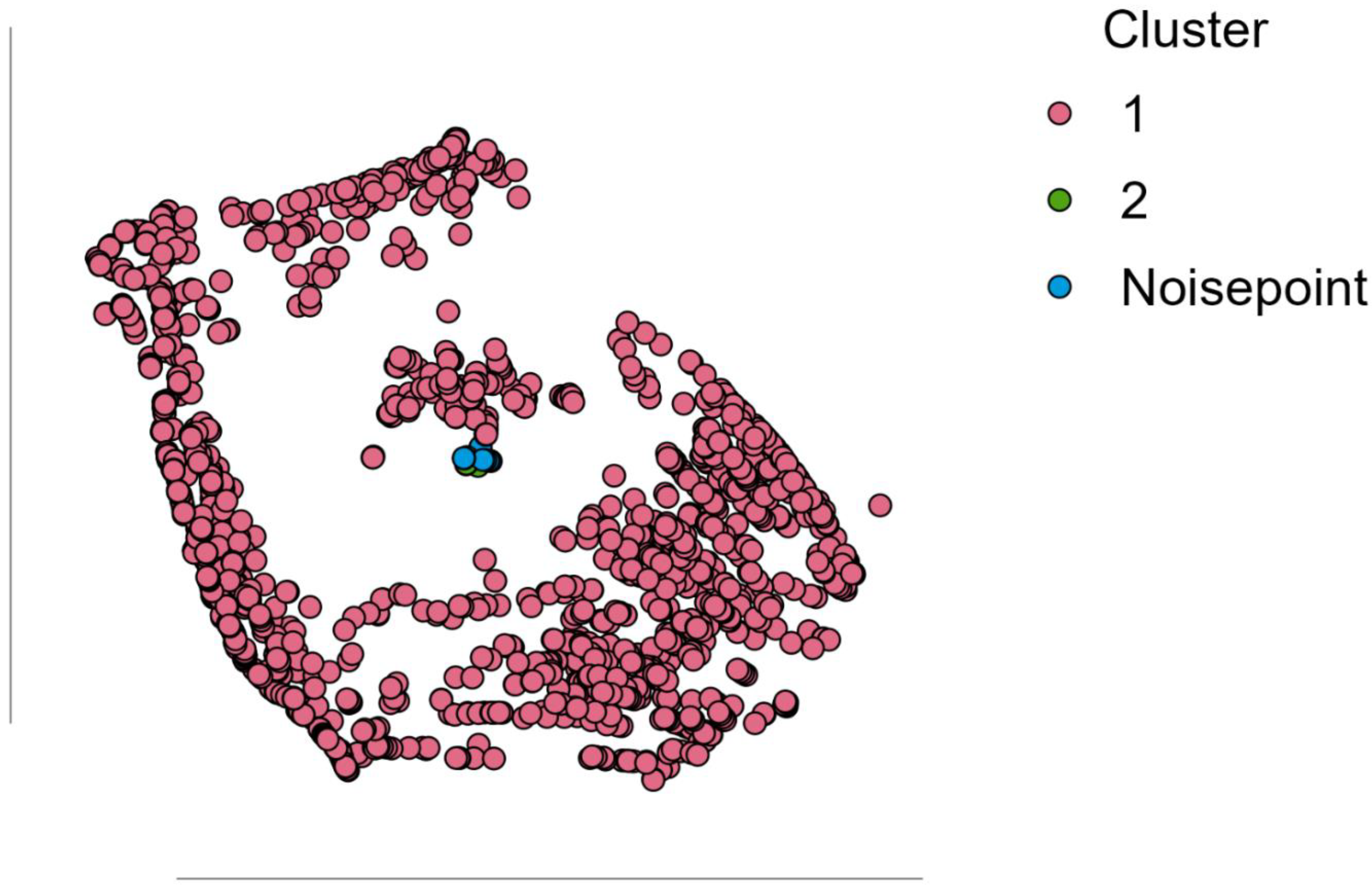
Figure 2.
Cluster mean.
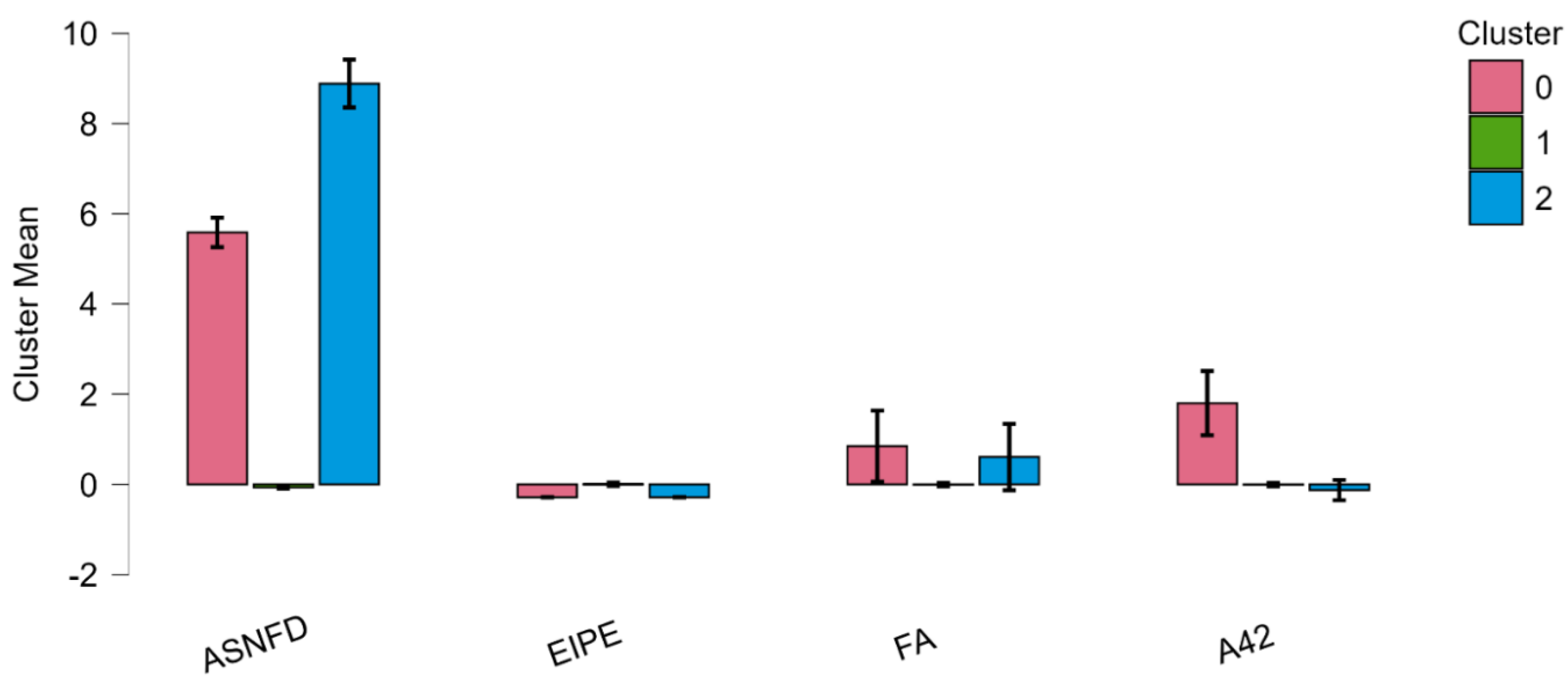
Figure 3.
Cluster matrix plot.
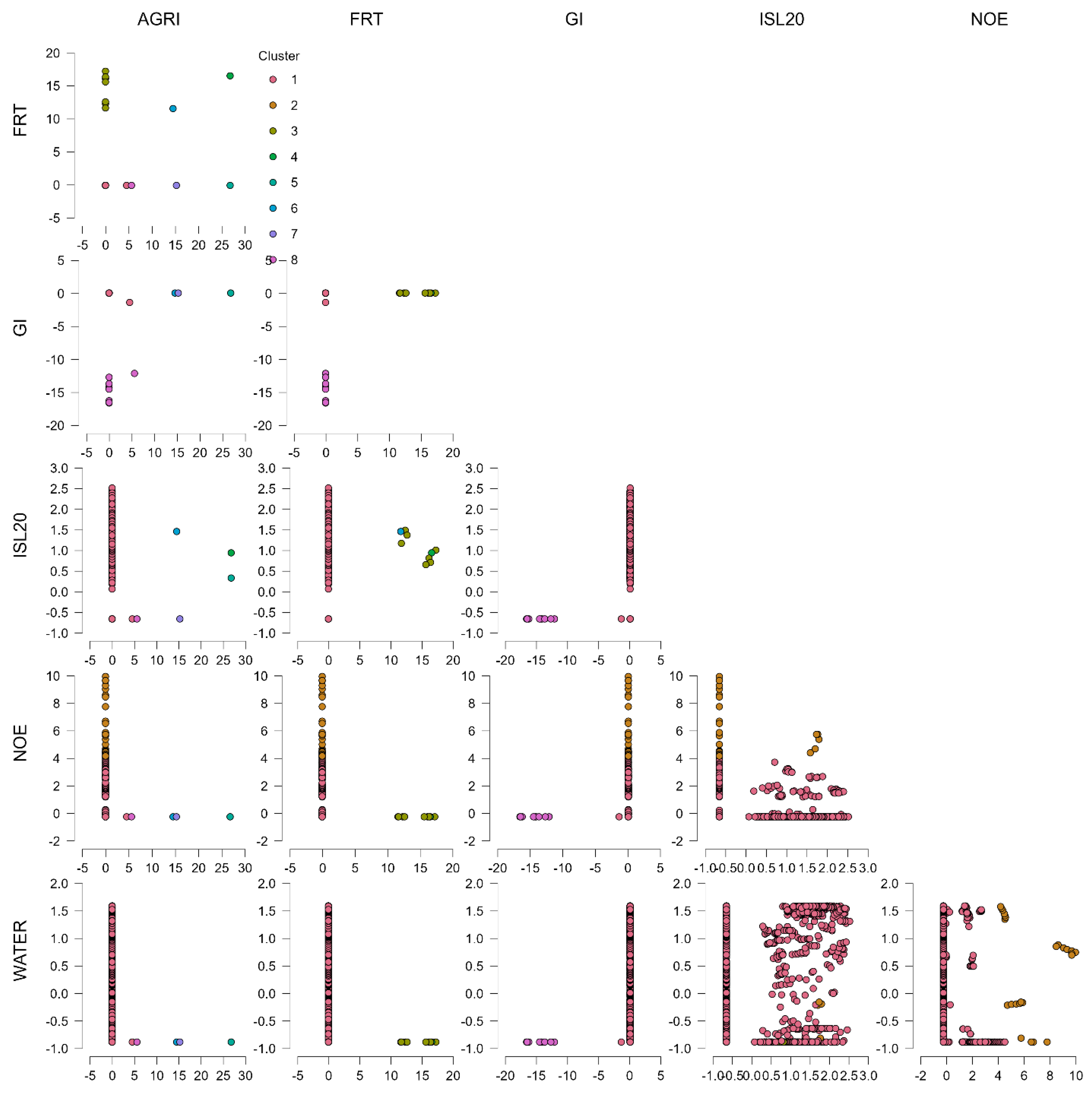
Figure 4.
Structure of hierarchical clustering with dendrogram.
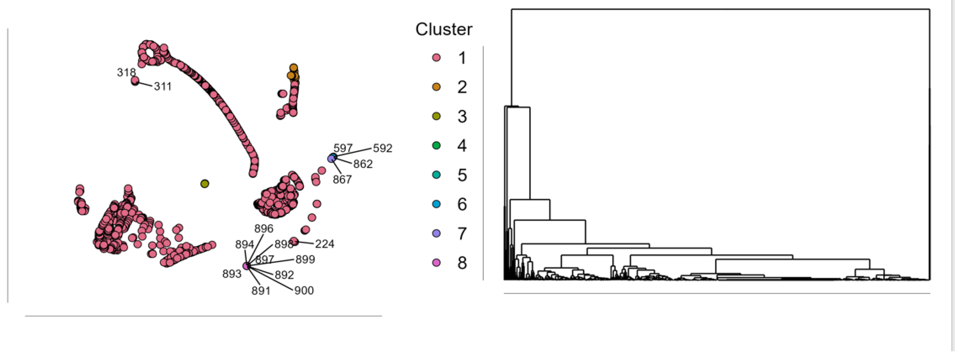
Figure 5.
Random Forest structure.
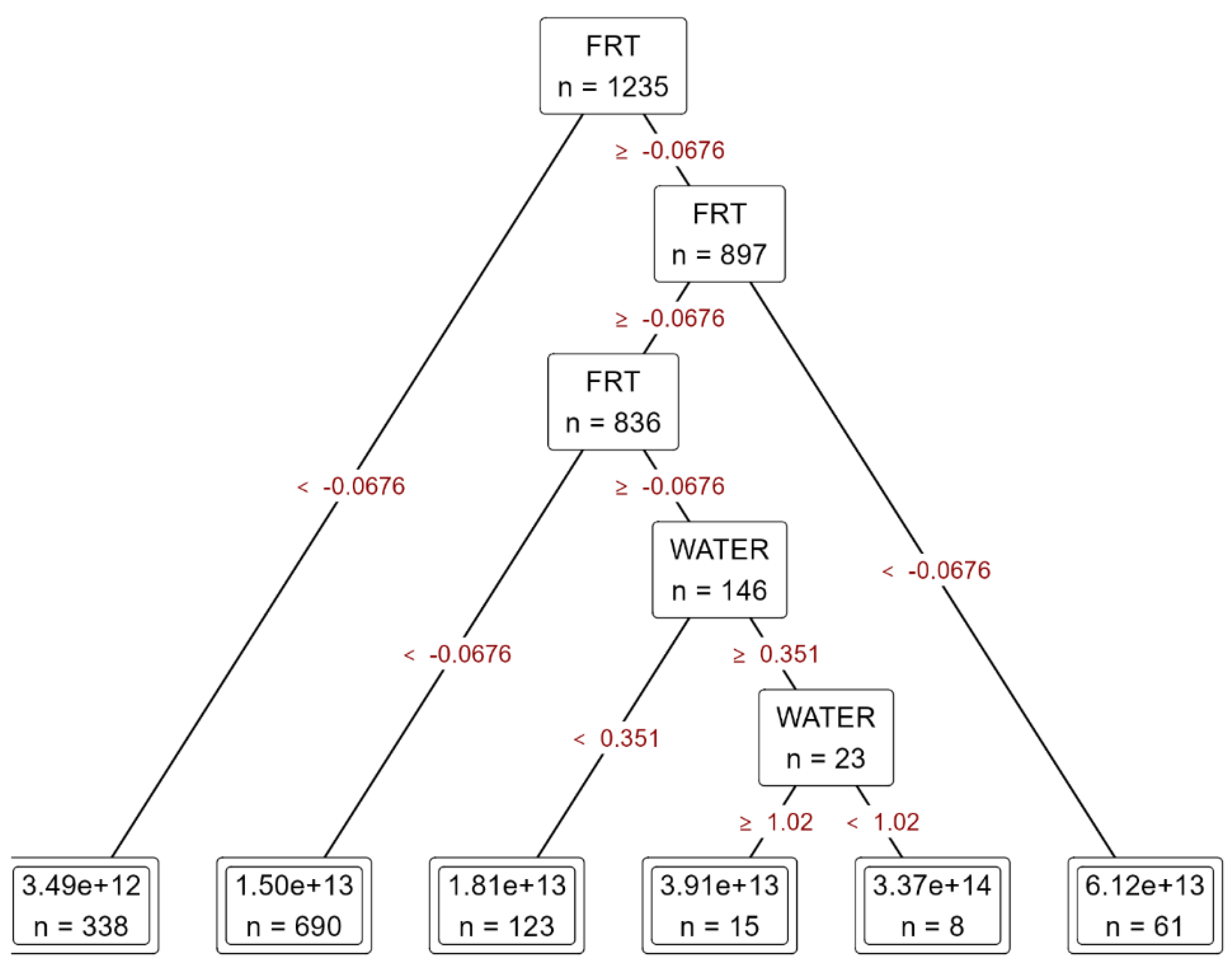
Figure 6.
Cluster mean.
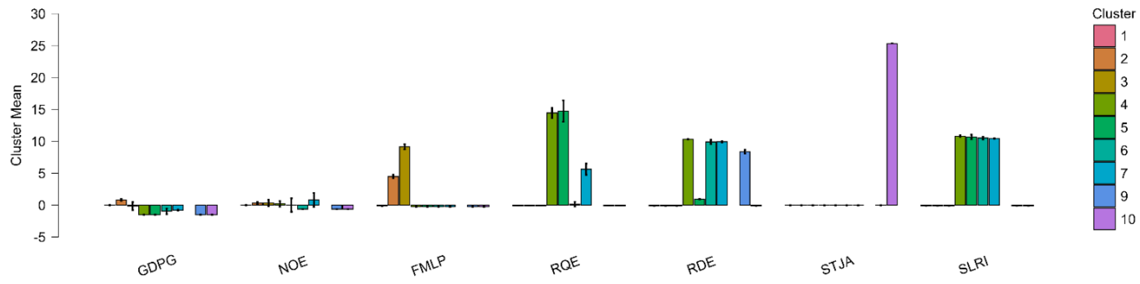
Figure 7.
Mean decrease in accuracy and total increase in node purity.
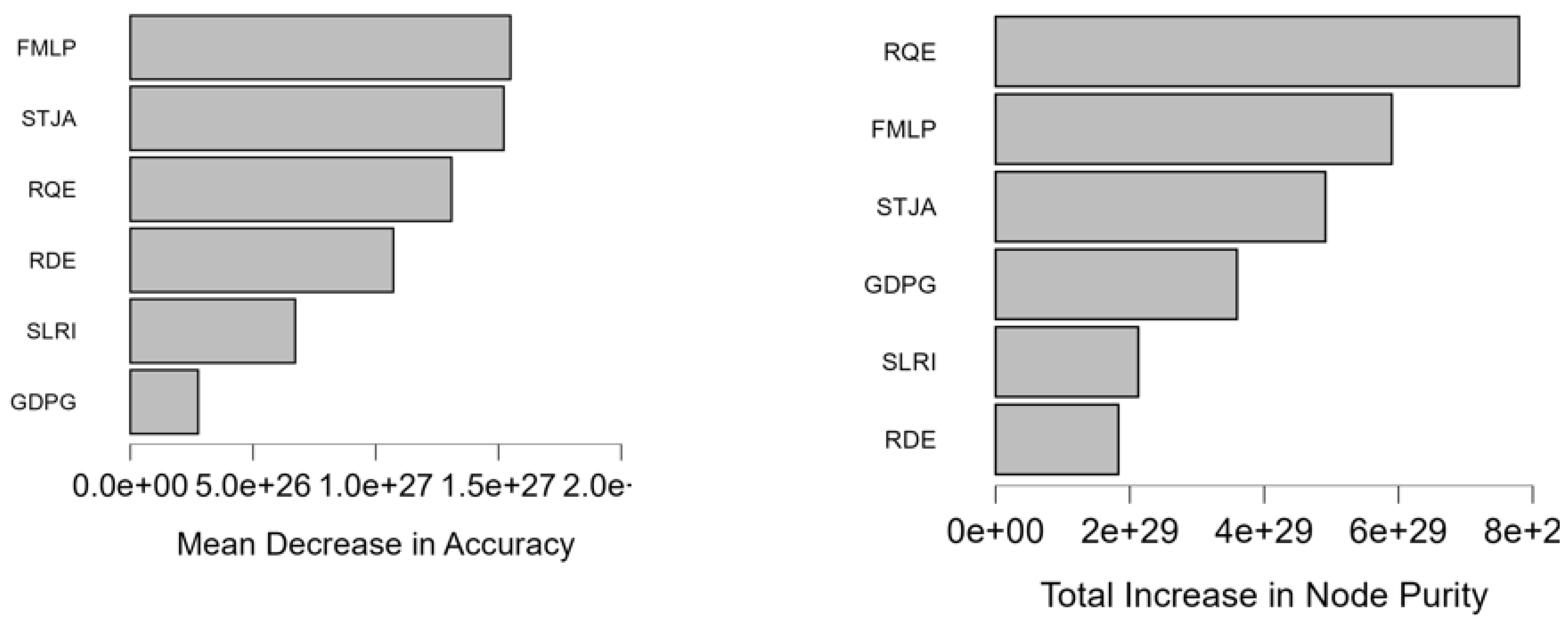

Table 1.
Variables of the model.
| Variable | Acronym | Description |
| Nitrous oxide emissions (metric tons of CO2 equivalent per capita) | NOE | This metric quantifies annual nitrous oxide (N₂O) emissions from agriculture, energy, waste, and industry, excluding LULUCF. Emissions are converted to carbon dioxide equivalents (CO₂e) using Global Warming Potential (GWP) factors from the IPCC’s Fifth Assessment Report (AR5), ensuring consistency in climate impact assessments. |
| Adjusted savings: net forest depletion (% of GNI) | ASNFD | Net forest depletion is determined by multiplying unit resource rents by the amount of roundwood harvested beyond natural forest growth. This metric reflects the economic cost of unsustainable logging, highlighting the depletion of forest resources beyond their regeneration capacity. By assessing the gap between harvest rates and natural growth, it provides insight into forest sustainability and the long-term environmental and economic impacts of excessive resource extraction. |
| Energy intensity level of primary energy (MJ/$2017 PPP GDP) | EIPE | The energy intensity level of primary energy measures the ratio of energy supply to GDP at purchasing power parity. It reflects the amount of energy required to produce one unit of economic output. A lower energy intensity indicates greater efficiency, meaning less energy is consumed per unit of output. This metric is crucial for assessing energy efficiency and sustainability in economic growth, guiding policies toward reduced energy consumption and improved resource management. |
| Forest area (% of land area) | FA | Forest area refers to land covered by natural or planted trees reaching at least 5 meters in height, regardless of productivity. It excludes tree stands within agricultural systems, such as fruit plantations and agroforestry, as well as trees in urban parks and gardens. This definition helps distinguish forest ecosystems from other tree-covered landscapes, ensuring accurate assessments of forest resources for environmental monitoring, conservation efforts, and sustainable land management. |
| Annualized average growth rate in per capita real survey mean consumption or income, total population (%) | AGRI | The welfare aggregate growth rate measures the annualized average increase in per capita real consumption or income for the total population over approximately five years. Derived from household surveys, this metric reflects overall economic well-being and living standards. By tracking changes in consumption or income, it provides insights into economic growth, poverty reduction, and inequality, helping policymakers assess the effectiveness of development strategies and social programs. |
| Fertility rate, total (births per woman) | FRT | The total fertility rate estimates the number of children a woman would have if she lived through her reproductive years and experienced the age-specific fertility rates of a given year. This measure reflects reproductive behavior and population growth trends, serving as a key demographic indicator. It helps policymakers assess fertility patterns, plan for future population changes, and develop strategies for healthcare, education, and economic development based on projected birth rates. |
| Gini index | GI | The Gini index quantifies income or consumption inequality within an economy, indicating how far distribution deviates from perfect equality. A value of 0 signifies complete equality, where everyone has the same income, while a value of 100 represents total inequality, where one individual holds all the income. This metric is widely used to assess economic disparity, helping policymakers evaluate social equity, design welfare programs, and track progress in reducing income inequality over time. |
| Income share held by lowest 20% | ISL20 | The percentage share of income or consumption represents the portion received by specific population subgroups, categorized by deciles or quintiles. This measure helps analyze income distribution and economic inequality. Due to rounding, the total percentage across quintiles may not always sum to 100. By assessing these shares, policymakers and researchers can evaluate disparities, monitor economic trends, and design policies to promote fairer income distribution and social equity. |
| People using safely managed drinking water services (% of population) | WATER |
This metric measures the percentage of people using improved drinking water sources that are accessible on-site, available when needed, and free from fecal or harmful chemical contamination. Improved sources include piped water, boreholes, tubewells, protected wells and springs, as well as packaged or delivered water. Ensuring access to safe drinking water is crucial for public health, reducing waterborne diseases, and supporting sustainable development and well-being in communities worldwide. |
| GDP growth (annual %) | GDPG | The annual GDP growth rate measures the percentage increase in GDP at market prices, based on constant local currency. Aggregates use constant 2010 U.S. dollars. GDP represents the total gross value added by resident producers, including product taxes and excluding subsidies. It does not account for asset depreciation or natural resource depletion. This indicator helps assess economic performance, guiding policymakers in evaluating growth trends and formulating development strategies. |
| Ratio of female to male labor force participation rate (%) (modeled ILO estimate) | FMLP | The labor force participation rate measures the percentage of people aged 15 and older who are economically active, contributing labor to goods and services production. The female-to-male participation ratio is calculated by dividing the female labor force participation rate by the male rate and multiplying by 100. This metric helps assess gender disparities in employment, informing policies on workforce inclusion and economic development. |
| Regulatory Quality: Estimate | RQE | Regulatory quality assesses a government's ability to develop and enforce effective policies that support private sector growth. It reflects the efficiency, fairness, and stability of regulations impacting businesses and economic activities. Strong regulatory frameworks encourage investment and economic development |
| Research and development expenditure (% of GDP) | RDE | Gross domestic R&D expenditures measure the percentage of GDP spent on research and development, including both capital and current costs. These expenditures span four key sectors: business enterprise, government, higher education, and private non-profit. R&D activities encompass basic research, applied research, and experimental development. This indicator reflects a country's commitment to innovation, technological progress, and economic growth, guiding policy decisions on science and technology investment. |
| Scientific and technical journal articles | STJA | Scientific and technical journal articles represent the number of published research papers in fields such as physics, biology, chemistry, mathematics, clinical medicine, biomedical research, engineering, technology, and earth and space sciences. This metric reflects a country's research output, scientific progress, and contributions to global knowledge. Tracking publication trends helps assess innovation, academic productivity, and the impact of research investments on technological and scientific advancements. |
| Strength of legal rights index (0=weak to 12=strong) | SLRI | The Strength of Legal Rights Index assesses how well collateral and bankruptcy laws protect borrowers and lenders, promoting secure lending. It ranges from 0 to 12, with higher scores indicating stronger legal frameworks that enhance access to credit. A well-designed legal system fosters financial stability, encouraging investment and economic growth. This index helps policymakers and investors evaluate the effectiveness of credit laws in supporting a robust financial environment. |
Table 2.
Results of the panel data regressions.
| Fixed-effects, using 1930 observations | Random-effects (GLS), using 1930 observations | |||||
| Coefficient | Std. Error | t-ratio | Coefficient | Std. Error | z | |
| Constant | -1537.59* | 875.027 | -1.757 | -356.662 | 261.750 | -1.363 |
| ASFND | 388.620*** | 111.720 | 3.479 | 226.326 | 63.2516 | 3.578 |
| EIPE | -23.9106*** | 6.61187 | -3.616 | -16.2174 | 5.23974 | -3.095 |
| FA | 45.1940* | 26.8273 | 1.685 | 11.7874 | 6.23894 | 1.889 |
| Statistics | Mean dependent var | 123.4940 | Mean dependent var | 123.4940 | ||
| Sum squared resid | 4.20e+10 | Sum squared resid | 4.48e+10 | |||
| LSDV R-squared | 0.073296 | Log-likelihood | -19105.89 | |||
| LSDV F(195, 1734) | 0.703319 | Schwarz criterion | 38242.05 | |||
| Log-likelihood | -19041.77 | rho | -0.092917 | |||
| Schwarz criterion | 39566.33 | S.D. dependent var | 4844.417 | |||
| rho | -0.092917 | S.E. of regression | 4823.555 | |||
| S.D. dependent var | 4844.417 | Akaike criterion | 38219.79 | |||
| S.E. of regression | 4918.738 | Hannan-Quinn | 38227.98 | |||
| Within R-squared | 0.012731 | Durbin-Watson | 2.166681 | |||
| P-value(F) | 0.999081 | |||||
| Akaike criterion | 38475.54 | |||||
| Hannan-Quinn | 38876.78 | |||||
| Durbin-Watson | 2.166681 | |||||
| Tests | Joint test on named regressors - Test statistic: F(3, 1734) = 7.45344 with p-value = P(F(3, 1734) > 7.45344) = 5.85983e-05 Test for differing group intercepts - Null hypothesis: The groups have a common intercept Test statistic: F(192, 1734) = 0.615528 with p-value = P(F(192, 1734) > 0.615528) = 0.999987 |
'Between' variance = 2.39935e+006 'Within' variance = 2.1737e+007 theta used for quasi-demeaning = 0.31056 Joint test on named regressors - Asymptotic test statistic: Chi-square(3) = 19.4119 with p-value = 0.000224696 Breusch-Pagan test - Null hypothesis: Variance of the unit-specific error = 0 Asymptotic test statistic: Chi-square(1) = 16.8159 with p-value = 4.11866e-05 Hausman test - Null hypothesis: GLS estimates are consistent Asymptotic test statistic: Chi-square(3) = 7.93254 with p-value = 0.0474267 |
||||
Table 3.
Statists of Machine Learning algorithms for clustering.
| Density-Based | Fuzzy C-Means | Hierarchical | Neighborhood-Based | |
| Maximum diameter | 9.377 | 8.730 | 4.851 | 6.373 |
| Minimum separation | 0.626 | 0.003 | 0.233 | 0.008 |
| Pearson's γ | 0.495 | 0.312 | 0.646 | 0.415 |
| Dunn index | 0.067 | 3.104×10⁻⁴ | 0.048 | 0.001 |
| Entropy | 0.059 | 2.043 | 0.810 | 2.060 |
| Calinski-Harabasz index | 157.775 | 331.266 | 276.568 | 966.206 |
| Cluster | 2 | 9 | 10 | 10 |
Table 4.
Normalized Results.
| Maximum Diameter | Minimum Separation | Pearson's γ | Dunn Index | Entropy | Calinski-Harabasz | |
| Density-Based | 0.000 | 1.000 | 0.549 | 1.000 | 1.000 | 0.000 |
| Fuzzy C-Means | 0.182 | 0.000 | 0.000 | 0.000 | 0.010 | 0.212 |
| Hierarchical | 1.000 | 0.368 | 1.000 | 0.716 | 0.621 | 0.151 |
| Neighborhood-Based | 0.398 | 0.008 | 0.308 | 0.010 | 0.000 | 1.000 |
Table 5.
Statistical results. .
| Algorithms | MSE | MSE(scaled) | RMSE | MAE / MAD | R² |
| Boosting Regression | 3,19843E+40 | 1766 | 56554677919974.9 | 27495573662284.5 | 0.013 |
| Decision Tree | 4,67384E+41 | 1279 | 6,83655E+13 | 27884948108250.7 | 0.129 |
| K-Nearest Neighbors | 3,30741E+41 | 1143 | 57510088985819.6 | 20214183938440.9 | 0.182 |
| Linear Regression | 4,2826E+41 | 1832 | 65441594103392.5 | 30141169680947.5 | 0.007 |
| Ranfom Forest | 3,88921E+41 | 1235 | 62363539135740.7 | 25751902907169.1 | 0.145 |
| Regularized Linear | 3,06909E+40 | 1911 | 55399392260728.8 | 27330517747988.2 | 0.002 |
| Support Vector Machine | 2,73796E+41 | 1715 | 52325517606098.3 | 12483937823834.3 | 0.02 |
Table 6.
Mean Dropout Loss
| Mean dropout loss | |||
| FA | 8.211×10+13 | ||
| EIPE | 7.093×10+13 | ||
| ASNFD | 5.537×10+13 | ||
| Note. Mean dropout loss (defined as root mean squared error (RMSE)) is based on 50 permutations. | |||
Table 7.
Additive Explanations for Predictions of Test Set Cases
| Case | Predicted | Base | ASNFD | EIPE | FA | ||||||
| 1 | 0.190 | 1.618×10+13 | 91.144 | -8.977×10+12 | -7.204×10+12 | ||||||
| 2 | 9.718×10+13 | 1.618×10+13 | -5.657×10+11 | -3.297×10+12 | 8.486×10+13 | ||||||
| 3 | 9.718×10+13 | 1.618×10+13 | -2.667×10+11 | -3.176×10+12 | 8.444×10+13 | ||||||
| 4 | 0.251 | 1.618×10+13 | 9.154×10+11 | -5.505×10+12 | -1.159×10+13 | ||||||
| 5 | 0.251 | 1.618×10+13 | 9.154×10+11 | -5.505×10+12 | -1.159×10+13 | ||||||
| Note. Displayed values represent feature contributions to the predicted value without features (column 'Base') for the test set. | |||||||||||
Table 8.
Results of the panel data estimations.
| Fixed-effects, using 1930 observations | Random-effects (GLS), using 1930 observations | |||||
| Coefficient | Std. Error | t-ratio | Coefficient | Std. Error | z | |
| Constant | 1454.83*** | 170.230 | 8.546 | 899.333*** | 262.237 | 3.429 |
| AGRI | 472.423*** | 79.2103 | 5.964 | 586.143*** | 74.9708 | 7.818 |
| FRT | 6.80979*** | 0.409731 | 16.62 | 6.73673*** | 0.390629 | 17.25 |
| GI | -56.4683*** | 18.2848 | -3.088 | -48.0761*** | 15.3428 | -3.133 |
| ISL20 | 325.574*** | 101.327 | 3.213 | 285.434*** | 84.3385 | 3.384 |
| WATER | -31.6670*** | 1.93732 | -16.35 | -21.4558*** | 1.52574 | -14.06 |
| Statistics | Mean dependent var | 123.4940 | Mean dependent var | 123.4940 | ||
| Sum squared resid | 3.30e+10 | Sum squared resid | 3.95e+10 | |||
| LSDV R-squared | 0.270528 | Log-likelihood | -18984.86 | |||
| LSDV F(197, 1732) | 3.260515 | Schwarz criterion | 38015.10 | |||
| Log-likelihood | -18810.83 | rho | -0.053556 | |||
| Schwarz criterion | 39119.58 | S.D. dependent var | 4844.417 | |||
| rho | -0.053556 | S.E. of regression | 4532.691 | |||
| S.D. dependent var | 4844.417 | Akaike criterion | 37981.71 | |||
| S.E. of regression | 4532.691 | Hannan-Quinn | 37993.99 | |||
| Within R-squared | 37981.71 | Durbin-Watson | 2.027854 | |||
| P-value(F) | 37993.99 | |||||
| Akaike criterion | 2.027854 | |||||
| Hannan-Quinn | 4844.417 | |||||
| Durbin-Watson | 4532.691 | |||||
| Tests | Joint test on named regressors - Test statistic: F(5, 1732) = 99.3334 with p-value = P(F(5, 1732) > 99.3334) = 3.04478e-92 Test for differing group intercepts - Null hypothesis: The groups have a common intercept Test statistic: F(192, 1732) = 0.942888 with p-value = P(F(192, 1732) > 0.942888) = 0.696184 |
'Between' variance = 8.53727e+006 'Within' variance = 1.71106e+007 theta used for quasi-demeaning = 0.591392 Joint test on named regressors - Asymptotic test statistic: Chi-square(5) = 461.246 with p-value = 1.84191e-97 Breusch-Pagan test - Null hypothesis: Variance of the unit-specific error = 0 Asymptotic test statistic: Chi-square(1) = 58.3018 with p-value = 2.24841e-14 Hausman test - Null hypothesis: GLS estimates are consistent Asymptotic test statistic: Chi-square(5) = 94.715 with p-value = 6.85546e-19 |
||||
Table 9.
Statistical results.
| Neighborhood-Based | Density-Based | Fuzzy C-Means | Hierarchical | Random Forest | |
| Maximum diameter | 20.291 | 35.700 | 35.700 | 7.167 | 35.700 |
| Minimum separation | 0.008 | 0.268 | 0.014 | 0.855 | 9.159×10⁻¹⁶ |
| Pearson's γ | 0.413 | 0.777 | 0.200 | 0.751 | 0.042 |
| Dunn index | 4.133×10⁻⁴ | 0.008 | 3.914×10⁻⁴ | 0.119 | 2.566×10⁻¹⁷ |
| Entropy | 1.679 | 0.067 | 1.138 | 0.143 | 2.054 |
| Calinski-Harabasz index | 1.943.052 | 351.756 | 200.783 | 395.441 | 67.591 |
Table 10.
Cluster information.
| Cluster | 1 | 2 | 3 | 4 | 5 | 6 | 7 | 8 |
| Size | 1884 | 26 | 7 | 1 | 1 | 1 | 1 | 9 |
| Explained proportion within-cluster heterogeneity | 0.951 | 0.032 | 0.007 | 0.000 | 0.000 | 0.000 | 0.000 | 0.010 |
| Within sum of squares | 4.509.331 | 152.614 | 31.928 | 0.000 | 0.000 | 0.000 | 0.000 | 49.157 |
| Silhouette score | 0.727 | 0.526 | 0.801 | 0.000 | 0.000 | 0.000 | 0.000 | 0.811 |
| Note. The Between Sum of Squares of the 8 cluster model is 6830.97 | ||||||||
| Note. The Total Sum of Squares of the 8 cluster model is 11574 | ||||||||
Table 11.
Clusters.
| Annualized average growth rate in per capita real survey mean consumption or income, total population (%) | Fertility rate, total (births per woman) | Gini index | Income share held by lowest 20% | Nitrous oxide emissions (metric tons of CO2 equivalent per capita) | People using safely managed drinking water services (% of population) | |
| Cluster 1 | -0.046 | -0.068 | 0.068 | 9.487×10⁻⁴ | -0.087 | 0.003 |
| Cluster 2 | -0.048 | -0.068 | 0.069 | -0.200 | 6.491 | 0.428 |
| Cluster 3 | -0.048 | 14.549 | 0.069 | 1.035 | -0.240 | -0.881 |
| Cluster 4 | 26.764 | 16.532 | 0.069 | 0.946 | -0.240 | -0.881 |
| Cluster 5 | 26.764 | -0.068 | 0.069 | 0.335 | -0.240 | -0.881 |
| Cluster 6 | 14.484 | 11.568 | 0.069 | 1.463 | -0.240 | -0.881 |
| Cluster 7 | 15.204 | -0.068 | 0.069 | -0.656 | -0.240 | -0.881 |
| Cluster 8 | 0.573 | -0.068 | -14.517 | -0.656 | -0.240 | -0.881 |
Table 12.
Statistical results.
| MSE | MSE(scaled) | RMSE | MAE / MAD | R^2 | |
| Random Forest | 0.3600117698984846 | 0.4052044609665427 | 0.0 | 0.40304705986553213 | 1.0 |
| Boosting | 0.53508900985729 | 0.8131970260223048 | 0.32368112518096126 | 0.0 | 0.0473186119873817 |
| Decision Tree | 0.0 | 1.0 | 0.054866835868048414 | 0.5070895929367109 | 0.01892744479495268 |
| K-Nearest Neighbors | 0.42180373694276885 | 0.8155204460966542 | 0.12098647345216462 | 0.38438382120220915 | 0.04416403785488959 |
| Linear Regression | 0.0382521700750331 | 0.9223977695167287 | 0.6911298418038796 | 0.8766936557107904 | 0.0 |
| Regularized Linear | 0.9999999999999999 | 0.0 | 1.0 | 0.9999999999999999 | 0.0 |
| Support Vector Machine | 0.902898337501839 | 0.9423791821561338 | 0.8729590916197361 | 0.19592520124232793 | 0.0 |
Table 13.
Feature Importance Metrics
| Relative Importance | Mean dropout loss | ||||
| People using safely managed drinking water services (% of population) | 52.228 | 7.471×10+13 | |||
| Fertility rate, total (births per woman) | 36.154 | 7.710×10+13 | |||
| Income share held by lowest 20% | 7.708 | 6.167×10+13 | |||
| Gini index | 3.854 | 6.167×10+13 | |||
| Annualized average growth rate in per capita real survey mean consumption or income, total population (%) | 0.057 | 6.167×10+13 | |||
| Note. Mean dropout loss (defined as root mean squared error (RMSE)) is based on 50 permutations. | |||||
Table 14.
Additive Explanations for Predictions of Test Set Cases
| Case | Predicted | Base | Annualized average growth rate in per capita real survey mean consumption or income, total population (%) | Fertility rate, total (births per woman) | Gini index | Income share held by lowest 20% | People using safely managed drinking water services (% of population) | ||||||||
| 1 | 1.501×10+13 | 1.682×10+13 | 0.000 | 5.112×10+11 | 0.000 | 0.000 | -2.320×10+12 | ||||||||
| 2 | 1.501×10+13 | 1.682×10+13 | 0.000 | 5.112×10+11 | 0.000 | 0.000 | -2.320×10+12 | ||||||||
| 3 | 1.501×10+13 | 1.682×10+13 | 0.000 | -3.717×10+13 | 0.000 | 0.000 | 3.536×10+13 | ||||||||
| 4 | 3.491×10+12 | 1.682×10+13 | 0.000 | -4.869×10+13 | 0.000 | 0.000 | 3.536×10+13 | ||||||||
| 5 | 1.501×10+13 | 1.682×10+13 | 0.000 | -3.717×10+13 | 0.000 | 0.000 | 3.536×10+13 | ||||||||
| Note. Displayed values represent feature contributions to the predicted value without features (column 'Base') for the test set. | |||||||||||||||
Table 15.
Results of the panel data regressions.
| Fixed-effects, using 1930 observations | Random-effects (GLS), using 1930 observations | |||||
| Coefficient | Std. Error | t-ratio | Coefficient | Std. Error | z | |
| Constant | 556.472 | 320.867 | 1.734 | 103.524 | 216.422 | 0.4783 |
| GDPG | 164.956*** | 17.3297 | 9.519 | 145.221*** | 15.0543 | 9.647 |
| FMLP | -25.5933*** | 5.50773 | -4.647 | -11.6487*** | 3.43191 | -3.394 |
| RQE | 71.9341*** | 31.3453 | 2.295 | 51.2178*** | 16.4078 | 3.122 |
| RDE | 2127.27*** | 253.026 | 8.407 | 843.694*** | 143.536 | 5.878 |
| STJA | -0.018322** | 0.00601105 | -3.048 | -0.0070** | 0.00277893 | -2.553 |
| SLRI | -7.80164*** | 1.00910 | -7.731 | -2.39160*** | 0.594355 | -4.024 |
| Statistics | Mean dependent var | 123.4940 | Mean dependent var | 123.4940 | ||
| Sum squared resid | 3.84e+10 | Sum squared resid | 3.98e+10 | |||
| LSDV R-squared | 0.150695 | Log-likelihood | -18990.93 | |||
| LSDV F(198, 1731) | 1.551193 | Schwarz criterion | 38034.82 | |||
| Log-likelihood | -18957.61 | rho | -0.228742 | |||
| Schwarz criterion | 39420.70 | S.D. dependent var | 4844.417 | |||
| rho | -0.228742 | S.E. of regression | 4548.164 | |||
| S.D. dependent var | 4844.417 | Akaike criterion | 37995.86 | |||
| S.E. of regression | 4712.930 | Hannan-Quinn | 38010.19 | |||
| Within R-squared | 0.095188 | Durbin-Watson | 2.415716 | |||
| P-value(F) | 5.13e-06 | |||||
| Akaike criterion | 38313.21 | |||||
| Hannan-Quinn | 38720.59 | |||||
| Durbin-Watson | 2.415716 | |||||
| Tests | Joint test on named regressors - Test statistic: F(6, 1731) = 30.3509 with p-value = P(F(6, 1731) > 30.3509) = 8.76611e-35 Test for differing group intercepts - Null hypothesis: The groups have a common intercept Test statistic: F(192, 1731) = 0.316789 with p-value = P(F(192, 1731) > 0.316789) = 1 |
'Between' variance = 0 'Within' variance = 2.22117e+007 theta used for quasi-demeaning = 0 Joint test on named regressors - Asymptotic test statistic: Chi-square(6) = 264.345 with p-value = 3.51602e-54 Breusch-Pagan test - Null hypothesis: Variance of the unit-specific error = 0 Asymptotic test statistic: Chi-square(1) = 75.4695 with p-value = 3.71086e-18 Hausman test - Null hypothesis: GLS estimates are consistent Asymptotic test statistic: Chi-square(6) = 67.1804 with p-value = 1.54599e-12 |
||||
Table 16.
Normalized results.
| Density Based | Fuzzy C-Means | Hierarchical Clustering | Model Based | Neighborhood Based | Random Forest | |
| Maximum diameter | 0.06745352911624239 | 0.22273019387353776 | 0.014490492399853205 | 0.04702319565817511 | 0.015907641995282558 | 0.8812466415905428 |
| Minimum separation | 0.0043137529226470964 | 5,16E+10 | 0.0008921959227085836 | 9,76E+09 | 1,47E+09 | 9,95E-02 |
| Pearson's γ | 0.0016216319340663532 | 0.0013952893047397283 | 0.001445972702320808 | 0.0004108959502102246 | 0.0002271315632102517 | 0.0009254283837841031 |
| Dunn index | 0.0 | 0.0 | 0.0 | 0.0 | 0.0 | 0.0 |
| Entropy | 5,09E+10 | 0.012457710676359694 | 0.0002944686050318971 | 0.0031294973180489346 | 0.0015837832808435588 | 0.04218162278344975 |
| Calinski-Harabasz index | 1.0 | 0.9999999999999999 | 0.9999999999999999 | 1.0 | 1.0 | 1.0 |
Table 17.
Cluster Information
| Cluster | 1 | 2 | 3 | 4 | 5 | 6 | 7 | 8 | 9 | 10 | |||||||||||
| Size | 1864 | 32 | 9 | 6 | 2 | 3 | 6 | 1 | 4 | 3 | |||||||||||
| Explained proportion within-cluster heterogeneity | 0.977 | 0.010 | 0.005 | 0.002 | 6.879×10⁻⁴ | 2.534×10⁻⁴ | 0.005 | 0.000 | 9.414×10⁻⁵ | 9.886×10⁻²² | |||||||||||
| Within sum of squares | 4210.053 | 42.132 | 21.572 | 9.421 | 2.964 | 1.092 | 21.715 | 0.000 | 0.406 | 4.260×10⁻¹⁸ | |||||||||||
| Silhouette score | 0.611 | 0.653 | 0.559 | 0.795 | 0.745 | 0.830 | 0.572 | 0.000 | 0.921 | 1.000 | |||||||||||
| Note. The Between Sum of Squares of the 10 cluster model is 9193.65 | |||||||||||||||||||||
| Note. The Total Sum of Squares of the 10 cluster model is 13503 | |||||||||||||||||||||
Table 18.
Clusters.
| GDP growth (annual %) | Nitrous oxide emissions (metric tons of CO2 equivalent per capita) | Ratio of female to male labor force participation rate (%) (modeled ILO estimate) | Regulatory Quality: Estimate | Research and development expenditure (% of GDP) | Scientific and technical journal articles | Strength of legal rights index (0=weak to 12=strong) | |||||||||
| Cluster 1 | 0.003 | -0.008 | -0.118 | -0.081 | -0.103 | -0.039 | -0.095 | ||||||||
| Cluster 2 | 0.822 | 0.300 | 4.471 | -0.081 | -0.103 | -0.039 | -0.095 | ||||||||
| Cluster 3 | -0.165 | 0.318 | 9.127 | -0.081 | -0.103 | -0.039 | -0.095 | ||||||||
| Cluster 4 | -1.505 | 0.210 | -0.240 | 14.445 | 10.327 | -0.039 | 10.806 | ||||||||
| Cluster 5 | -1.505 | -0.004 | -0.240 | 14.747 | 0.936 | -0.039 | 10.685 | ||||||||
| Cluster 6 | -0.982 | -0.644 | -0.240 | 0.140 | 9.909 | -0.039 | 10.512 | ||||||||
| Cluster 7 | -0.797 | 0.830 | -0.240 | 5.621 | 9.926 | -0.039 | 10.409 | ||||||||
| Cluster 8 | -0.776 | 2.309 | -0.240 | 4.690 | 9.960 | -0.039 | 0.963 | ||||||||
| Cluster 9 | -1.505 | -0.644 | -0.240 | -0.081 | 8.376 | -0.039 | -0.095 | ||||||||
| Cluster 10 | -1.505 | -0.644 | -0.240 | -0.081 | -0.103 | 25.338 | -0.095 | ||||||||
Table 19.
Statistical Results.
| MSE | MSE(scaled) | RMSE | MAE / MAD | R² | |
| Boosting | 0.9728629579375847 | 0.7763313609467455 | 0.8359913803089771 | 0.7568395879174474 | 0.09583333333333335 |
| Decision Tree | 0.7053692576080636 | 0.6248520710059171 | 0.0 | 0.2360953723670376 | 0.2 |
| K-Nearest Neighbors | 0.8914518317503393 | 0.7136094674556213 | 0.5943462348840258 | 0.9127409854532011 | 0.13333333333333333 |
| Linear Regression | 0.9340957549912774 | 0.8520710059171599 | 0.719097048440756 | 0.8641982435387621 | 0.05416666666666666 |
| Random Forest | 0.0 | 0.0 | 1.0 | 0.6100728056507307 | 10.000.000.000.000.000 |
| Regularized Linear | 0.9592944369063772 | 10.000.000.000.000.000 | 0.7917614846829375 | 1.0 | 0.0 |
| Support Vector Machine | 1.0 | 0.9810650887573964 | 0.913767544533286 | 0.0 | 0.004166666666666666 |
Table 20.
Mean decreased in accuracy and total increase in node purity.
| Mean decrease in accuracy | Total increase in node purity | |
| Regulatory Quality: Estimate | 2.195×10+27 | 6.433×10+29 |
| Ratio of female to male labor force participation rate (%) (modeled ILO estimate) | 2.076×10+27 | 5.768×10+29 |
| Scientific and technical journal articles | 2.171×10+27 | 4.340×10+29 |
| GDP growth (annual %) | 3.630×10+26 | 3.111×10+29 |
| Scientific and technical journal articles | 1.153×10+27 | 2.296×10+29 |
| Research and development expenditure (% of GDP) | 1.385×10+27 | 1.891×10+29 |
Disclaimer/Publisher’s Note: The statements, opinions and data contained in all publications are solely those of the individual author(s) and contributor(s) and not of MDPI and/or the editor(s). MDPI and/or the editor(s) disclaim responsibility for any injury to people or property resulting from any ideas, methods, instructions or products referred to in the content. |
© 2025 by the authors. Licensee MDPI, Basel, Switzerland. This article is an open access article distributed under the terms and conditions of the Creative Commons Attribution (CC BY) license (http://creativecommons.org/licenses/by/4.0/).
Copyright: This open access article is published under a Creative Commons CC BY 4.0 license, which permit the free download, distribution, and reuse, provided that the author and preprint are cited in any reuse.


