
Submitted:
24 April 2024
Posted:
28 April 2024
You are already at the latest version
Abstract
This study employs the reflection symmetry decomposition (RSD) method to extract polarization scattering features from ground object images, aiming to determine the optimal data input scheme for deep learning networks in polarimetric synthetic aperture radar classification. Eight distinct polarizing feature combinations are designed, and the classification accuracy of various approaches is evaluated using the classic convolutional neural networks(CNNs) AlexNet and VGG16. The findings reveal that the commonly employed 6-parameter input scheme, favored by many researchers, lacks the comprehensive utilization of polarization information and warrants attention. Intriguingly, leveraging the complete 9-parameter input scheme based on the polarization coherence matrix results in improved classification accuracy. Furthermore, the input scheme incorporating all 21 parameters from the RSD and polarization coherence matrix notably enhances overall accuracy and the Kappa coefficient compared to the other 7 schemes. This comprehensive approach maximizes the utilization of polarization scattering information from ground objects, emerging as the most effective CNN input data scheme in this study. Additionally, the classification performance using the second and third component total power values (P2 and P3) from the RSD surpasses the approach utilizing surface scattering power value (PS) and secondary scattering power value (PD) from the same decomposition.
Keywords:
polarimetric synthetic aperture radar (PolSAR)
; Deep learning
; Reflection Symmetric Decomposition (RSD)
; Input scheme
; Land classification
; Polarization feature extraction
; Convolutional Neural Network (CNN)
1. Introduction
Polarimetric synthetic aperture radar (PolSAR) possesses the capability to capture the complete polarized scattering characteristics of ground objects under diverse environmental conditions, making it applicable in various remote sensing scenarios [1,2,3]. Unlike conventional single-polarization SAR, PolSAR actively retrieves polarization information from surface scattering, offering a larger set of parameters to characterize electromagnetic scattering properties. For effective classification of polarimetric SAR data, these polarization features from PolSAR images must be comprehensively explored and leveraged within widely adopted deep learning algorithms.
Currently, PolSAR classification methods can be broadly categorized into three groups: 1. Polarimetric decomposition features: In this approach, PolSAR images undergo decomposition into polarimetric components, directly extracting the scattering characteristics of target objects. Common methods include Freeman decomposition [4], Cloude-Potier decomposition [5], Huynen decomposition [6], and others. 2. Statistical distribution characteristics: Classification is based on the statistical distribution characteristics of PolSAR data, with commonly used algorithms such as Wishart classification [7]. 3. Deep learning methods: With the rapid evolution of deep learning approaches, various methods have been introduced into PolSAR image classification [8,9,10]. The incorporation of multiple convolutional layers allows deep learning models to effectively extract high-level features, enhancing overall classification performance. Despite promising results achieved by researchers in PolSAR image classification using deep learning methods, the existing approaches have several limitations:
- Some algorithms stack and combine polarimetric decomposition features without considering the inherent limitations of the decomposition methods.
- Some methods normalize polarimetric features without accounting for the distribution characteristics of the data, often applying linear normalization methods to non-linear PolSAR data.
- Some methods employ different forms of CNN but overlook the complete scattering information and various polarimetric scattering characteristics in PolSAR images, utilizing incomplete polarized data as input for the network.
PolSAR images inherently contain multiple polarimetric features that can be utilized for CNN classification. Typically, the polarization coherency matrix (T) and the polarization covariance matrix (C) are widely used to represent polarimetric characteristics. Extracting valuable feature information for neural network classification involves decomposing PolSAR images into target polarimetric components using these matrices. Researchers have employed Sinclair scattering matrices [11], texture features [12,13], and spatial segmentation features [14] for PolSAR image classification. Pseudo-color synthesis, using decomposed target components, yields color characteristics of the targets, providing diverse information for PolSAR deep learning classification [15]. The challenge lies in effectively combining these features to enhance the accuracy of PolSAR classification.
With the advent of deep learning, researchers have explored various polarimetric data input schemes for PolSAR classification. Based on literature research, the most commonly employed input schemes are the 6-parameter method [18,19,20] and the 9-parameter method [21]. Additionally, some researchers [22] have integrated Cloude-Potier decomposition, Freeman-Durden decomposition, and Huynen decomposition, resulting in a total of 16 polarimetric features input schemes for PolSAR image classification. Nie et al. [10] utilized 12 polarimetric features from Freeman-Durden decomposition, Van Zyl decomposition [23], and Cloude-Potier decomposition, applying an enhanced learning framework for PolSAR image classification. While these methods have achieved high-accuracy classification of PolSAR images, increasing the number of polarimetric features does not consistently lead to improved classification accuracy [24] in PolSAR image classification. We attribute this to the following factors: 1) non-independence of polarimetric features obtained from polarimetric coherence/covariance matrices; 2) indiscriminate input of polarimetric features into the network, often increasing the difficulty of feature learning; 3) the associated increase in computational cost with an increased number of polarimetric features. Additionally, researchers have not thoroughly investigated the merits and limitations of polarimetric decomposition methods when utilizing polarimetric features. Instead, they directly applied components obtained from these algorithms without fully leveraging complete polarimetric decomposition to extract comprehensive backscattering information from objects. Consequently, the information at the data input stage remains incomplete, necessitating the combination of feature parameters at the input end of deep learning—a novel exploration in PolSAR deep learning classification.
PolSAR images encapsulate various original features of targets and extensive polarization information. This study adopts reflection symmetric decomposition (RSD), which can fully extract target polarization information. Polarimetric scattering features are extracted, and eight polarimetric feature input schemes are designed, comparing classification accuracy on the classical CNNs, AlexNet, and VGG16 is more common to analyze performance. The article conducts a comparative analysis based on various classification schemes employed by different scholars. By enhancing existing research schemes through feature extraction at the input stage and utilizing classic CNNs for PolSAR image classification, we achieve elevated classification accuracy and determine the optimal combination of polarimetric features as input schemes. The key conclusions of this study, with implications for researchers, are as follows:
- The classification performance utilizing total power values of the second component (P2) and the third component (P3) obtained from RSD surpasses schemes using surface scattering power value (PS) and double-bounce scattering power value (PD) from RSD. However, the optimal input scheme includes all P2, P3, PS, and PD.
- Regarding input schemes, in the face of limited computational resources, it is advisable to directly use the input scheme with all elements of the T matrix or utilize all components obtained through RSD, as both ensure the completeness of polarimetric information.
- The 21-channel input scheme should be used when computational resources are sufficient.
- The two classic CNNs employed, VGG16 and AlexNet, differ in depth. After five rounds of accuracy statistics, VGG16 demonstrates superior stability. While the 5-layer AlexNet neural network achieves high accuracy, it suggests that for PolSAR image classification using CNNs, an excessively deep network is unnecessary. In other words, VGG16 exhibits better stability, while the 5-layer AlexNet achieves higher accuracy.
The subsequent sections of the article are organized as follows: Part II primarily introduces classifiers for CNN classification and classic PolSAR decomposition methods. Part III presents the selected polar decomposition methods and the research plan. Part IV delves into experimental results and analysis. Finally, Part V elucidates the experimental conclusions and outlines prospects for future research endeavors.
2. Related Works
2.1. PolSAR Classification with CNN
The advent of computer hardware development has ushered in the era of deep learning, giving rise to networks such as AlexNet [25], GoogleNet [26], and the VGG series [27]. These networks have demonstrated exceptional performance across various domains. In a convolutional neural network, deep-level features of objects within images are extracted through convolutional layers, pooling layers, activation layers, and fully connected layers. This approach is more efficient than traditional methods and has been applied extensively [30,31,32,33].
The distinctive imaging mechanisms of PolSAR images render traditional methods for optical image classification obsolete. Challenges arise from differences in imaging geometry shape, object size, speckle noise, and non-linear normalization of PolSAR data. Scholars have turned to deep learning methods for PolSAR image classification, achieving notable success. Nie et al. [10] employed reinforcement learning to address low classification accuracy with limited samples. Ai et al. [28] proposed the use of gray-level co-occurrence matrices and conducted experiments on an enhanced convolutional autoencoder, achieving higher accuracy. Bi et al. [29] adopted a graph-based deep learning approach, enhancing classification performance by pairing and merging semi-supervised terms with limited samples.
2.2. Perform Polarization Decomposition Using a Scattering Mechanism
Target decomposition stands as a pivotal approach in the processing of PolSAR data, fundamentally expressing pixels as a weighted sum of diverse scattering mechanisms. In 1998, scholars Anthony Freeman and Stephen L. Durden introduced the initial model-based, non-coherent polarimetric decomposition algorithm [4], subsequently acknowledged as Freeman decomposition. Originally, Freeman’s decomposition aimed to provide viewers of multi-view SAR images with an intuitive means to distinguish the primary scattering mechanisms of objects. Freeman decomposition relies entirely on the back-scattering data observed by radar, with each component in its decomposition yielding a corresponding physical interpretation. Consequently, it earned its distinction as the first model-based, non-coherent polarimetric decomposition algorithm. The advent of Freeman decomposition marked a significant breakthrough. However, following its inception, extensive usage and further exploration unveiled three primary issues associated with its decomposition method: an overestimation of the volume scattering component, the presence of negative power components in the results, and the loss of polarization information. Notably, these three issues were found to be interrelated. For instance, the overestimation of the volume scattering component contributed to the existence of negative power values in subsequent surface scattering and double scattering components. Simultaneously, the loss of polarization information played a role in the inappropriate estimation of the power values of the volume scattering component.
In 2005, Yamaguchi et al. introduced a second model-based, non-coherent polarimetric decomposition algorithm [34], denoted as the Yamaguchi algorithm hereafter. This algorithm comprises four scattering components and introduced helix scattering as the fourth component, challenging the reflection symmetry assumption of Freeman decomposition and enhancing its applicability, particularly in urban area analysis. While this model-based approach opened avenues for improving the performance of non-coherent polarimetric decomposition algorithms through scattering model modifications, it did not offer a theoretical foundation for choosing helix scattering as the fourth component. According to the authors, the selection was more comparative and preferential. Notably, the innovations of Yamaguchi decomposition centered on the scattering model without altering the decomposition algorithm, which employed Freeman decomposition’s processing method. Despite exhibiting improved experimental results, the Yamaguchi algorithm retained issues like overestimation of volume scattering, negative power components, and loss of polarization information [35].
In the subsequent decade, numerous model-based, non-coherent polarimetric decomposition algorithms emerged. Reflection symmetry decomposition (RSD) [36,47] is a novel model-based, non-coherent polarimetric decomposition method that preserves polarization information. Demonstrating excellent algorithmic performance, RSD decomposes three components, all adhering to the mirror symmetry assumption. Notably, the original polarimetric coherence matrix can be fully reconstructed from RSD’s decomposition results, rendering it a comprehensive decomposition algorithm. The RSD algorithm employs an expanded set of polarimetric decomposition parameters, primarily involving unitary transformation, with superior mathematical properties and more expansive research possibilities compared to other decomposition algorithms. Leveraging these advantages, we adopt RSD as the polarimetric decomposition method for PolSAR images in this study.
3. Methods
This section outlines the experimental processing flow, covering radiometric calibration, polarization filtering, polarization feature extraction, and the configuration of CNNs and relevant parameters. It emphasizes the processing of PolSAR data and polarization features, providing insights into the basis and specific distribution of the chosen polarization data input scheme. The details are as follows:
3.1. Data Analysis and Feature Extraction
PolSAR data, represented by a Sinclair matrix under a single look, reflects polarimetric backscattering information related solely to the targets. The polarimetric scattering matrix can be expressed as follows:
Upon satisfying the reciprocity theorem, the polarization coherency matrix T is derived post multi-look processing, eliminating coherent speckle noise:
Among them,
k represents the scattering vector of the backscattering S matrix in the Pauli basis, where the superscript H denotes the Hermitian transpose. <•> represents an ensemble average. Additionally, the S-matrix is vectorized using the Lexicographic basis to obtain the polarimetric covariance matrix C, which can be converted back and forth between C and T. The T matrix is a positive semi-definite Hermitian matrix, which can be represented as a 9-dimensional real vector [T11, T22, T33, Re(T12), Re(T13), Re(T23), Im(T12), Im(T13), Im(T23)]. Tij represents the element in the i-th row and j-th column of the T matrix. Re(Tij) and Im(Tij) represent the real and imaginary parts of the Tij element, respectively.
Researchers have used this vector or its partial parameters for PolSAR image classification [18,19,20,21]. Additionally, the T matrix can undergo non-coherent polarimetric decomposition, yielding several scattering components with parameters utilized for PolSAR classification [10,22]. Furthermore, pseudocolored power values of the scattering components from polarimetric decomposition provide color information for features in PolSAR images.
3.2. Experimental Images and Preprocessing
The PolSAR images, acquired from the L1A-level standard single-look data of China’s GF-3 satellite, underwent polarization decomposition. The T matrix and all polarization feature parameters from RSD were obtained. Non-local means filtering [40], chosen for its superior effect after comparison with methods like mean filtering, median filtering, Lee filtering [38], and polarization whitening filtering [39], was employed.
3.3. PolSAR Classification Using Different Polarimetric Data Input Schemes
In PolSAR image classification, emphasis is often placed on the potential enhancement of classification accuracy through various deep learning modules, analyzing input values. However, attention to the polarization parameter schemes of the input is scarce. Effective feature combinations are crucial for PolSAR image classification, as different polarimetric scattering features can reflect object scattering characteristics from diverse perspectives.
While CNNs typically use only a subset of these features for training, limiting the utilization of polarization information, each pixel in PolSAR data can be represented by the T matrix—a fundamental form for PolSAR classification tasks.
Target decomposition, a primary approach in polarimetric SAR data processing, represents pixels as a weighted sum of several scattering mechanisms. In 1998, Freeman and Durden proposed the first model-based incoherent polarimetric decomposition algorithm [4], which had issues such as overestimation of volume scattering components, presence of negative power components, and loss of polarization information. In 2005, Yamaguchi et al. introduced the second model-based incoherent polarimetric decomposition algorithm [34]. Despite improvements in the scattering model, the decomposition algorithm itself still followed Freeman’s method, and issues of overestimation, negative power components, and loss of polarization information persisted [35].
Compared to several classic polar decomposition algorithms, RSD [36] possesses advantages such as no negative power components in the decomposition results, complete reconstruction of the original polarimetric covariance matrix, and structural conformity of the three components with the selected scattering model. By applying RSD, more polarimetric decomposition physical quantities can be obtained. The decomposition algorithm, mainly involving unitary transformation, exhibits better mathematical properties and more research possibilities compared to other methods. Hence, this study selects RSD as the polarimetric decomposition method for PolSAR imagery.
The polarized characteristics derived from reflected symmetry decomposition encompass surface scattering power (PV), secondary scattering power (PS), bulk scattering power (PD), the total power value of the second component of reflected symmetry decomposition (P2), and the total power value of the third component of reflected symmetry decomposition (P3). The value range for these components is [0, +∞). The doubled directional angle θ spans (-π/2, π/2], and the doubled helix angle φ covers [-π/4, π/4]. The power proportion of spherical scattering in the second component of reflected symmetry decomposition is denoted as x, and in the third component, it is denoted as y. Both x and y range from [0,1]. The phase of element a in the second component of reflected symmetry decomposition (T12) and the phase of element b in the third component of reflected symmetry decomposition (T12) both fall within the range of [-π, π] [47].
Before inputting these physical quantities into the CNN model, it is essential to normalize their ranges. In the T matrix, the total power value is normalized by converting Span to a unit of dB. The scattering power parameters T11, T22, T33, PS, PD, PV, P2, and P3 are all divided by Span to achieve normalization. The remaining components undergo maximum-minimum normalization, as indicated in Formula (3).
The correlation coefficients between channels T12, T23, and T23 in the T matrix are given by formulas (4), (5), and (6).
The normalized polarimetric feature parameters mentioned above are categorized into different input schemes following specified rules. First, as per references [18,19,20], the non-normalized total power (NonP0), T11, T22, T33, and the correlation coefficients coe12, coe13, coe23 between T12, T13, T23 channels form input scheme 1. Recognizing that the polarimetric total power Span is not normalized, normalized Span (P0) is adopted as research scheme 2. Subsequently, normalized T11 is added to research scheme 2 as research scheme 3. Considering that PS, PD, and PV are all polarization power values, these three physical quantities are replaced, resulting in research scheme 4. The decomposed total power values P2 and P3 obtained through reflection symmetry decomposition are used to substitute PS and PD in research scheme 4, resulting in research scheme 5. P2, P3, PS, and PD are simultaneously inputted into the CNN as research scheme 6. Furthermore, based on the research of related scholars, all elements of the T matrix, augmented with the normalized Span (P0), form research scheme 7. Finally, all reflection symmetry decomposition parameters after normalization constitute research scheme 8. The specific details of all eight polarization data input schemes are shown in Table 1.
3.4. Network Selection and Parameter Configuration, Loss Function, Evaluation Criteria
AlexNet and VGG16 are seminal networks in deep learning that demonstrate exceptional performance in image classification tasks. This paper opts for these two networks to validate the accuracy of each research scheme. The utilized AlexNet comprises 3 convolutional layers, one pooling layer, 3 fully connected layers, and one softmax layer. VGG16, on the other hand, integrates 13 convolutional layers, four max-pooling layers, three fully connected layers, and one softmax layer. Post-experimentation, within both networks, AlexNet and VGG16, the input data size is set at 4, where n represents the number of parameters in the polarized data input scheme. Employing the Kaiming initialization method [41], an initial learning rate of 0.1, decay rate of 0.1, weight initialization of 0.9, and weight decay coefficient of 0.0005 [42] are applied to achieve optimal training accuracy. The network utilizes the cross-entropy loss function, as expressed in Formula (7).
Here, M signifies the number of categories, yic represents the indicator function (0 or 1), and pic is the probability of observing the sample value. To quantitatively assess classification accuracy, five experiments are conducted on the classification results, utilizing average accuracy, highest overall accuracy, accuracy for each land cover type, and the Kappa coefficient.
3.5. Experimental Process
Figure 1 illustrates the process of employing CNN to classify eight polarimetric data input schemes. Initially, upon obtaining L1A level GF3 data, the original data undergoes radiometric calibration [37] and polarimetric filtering [40]. Subsequently, the processed data undergoes polarimetric decomposition to extract features characterizing the back-scattering information of the targets. Following different normalization rules, the data is segmented into eight polarimetric data input schemes. The acquired datasets are then trained and validated using CNN, saving parameters such as weights and biases. Finally, the trained model classifies the entire image, leveraging convolution to ascertain feature value sizes. The fully connected layer and the softmax function are employed to determine the class to which the targets belong. The classification results are filled into an empty matrix of the same size as the predicted image, yielding the complete image classification results.
4. Experimental Results and Analysis
In this section, we conducted experiments employing various research approaches with AlexNet and VGG16, systematically comparing the accuracy variations among them. For training and testing, four scenes of high-resolution polarimetric Synthetic Aperture Radar (SAR) images from the Yellow River Delta area, acquired by the GF3 satellite, were employed. All experiments were executed on a single GeForce 3060Ti GPU with the PyTorch framework, and the results were derived from five independent trials.
4.1. Data Explanation
GF-3 stands as China’s first C-band high-resolution fully-polarimetric SAR, widely applied owing to its diverse imaging modes [43,44,45]. Particularly, the full-polarimetric imaging mode I (QPSI) prove suitable for large-scale land cover investigations. The Yellow River Delta, selected as the research area based on field investigations, provided data obtained from the China Ocean Satellite Data Service System [46]. Four images were utilized: two taken on September 14, 2021(7882*9072 pixels,7882*9070 pixels respectively), one on October 13, 2021(6526*7317 pixels), and one on October 12, 2017(6014*7637 pixels). The initial three images were allocated for training, while the last image served as the test set. All images, acquired via the QPSI imaging mode, spanned an imaging range of (118°33′-119°20′ E, 37°35′-38°12′ N), with an incidence angle range of 30.97°-37.71°. Table 2 provides specific details and applications of the images, with the test image size set at 6014 *7637 pixels.
After field investigations, the primary land cover types in the research area were identified as nearshore water, seawater, spartina alterniflora, tamarix, reed, and tidal flats. Figure 2 illustrates pseudo-colored composites of PS, PD, and PV in the Yellow River Delta region and the ground truth map.
In this study, based on field investigations, the land cover types in the Yellow River Delta were classified into seven categories: nearshore water, seawater, spartina alterniflora, tamarix, reed, tidal flat, and suaeda salsa, labeled as numbers 1 to 7, respectively. In three training images, specific areas for each land cover type were chosen based on field investigations. Within these areas, 1000 samples were randomly selected, with 800 used for training and 200 for validation. The distribution of data samples is detailed in Table 3.
For test samples, 1000 samples for each land cover type on the test image were randomly selected. These samples constituted the test set, inputted into the trained model for testing. The classification results for the entire image were provided simultaneously, accompanied by an evaluation of the network model’s classification performance and the various polarimetric data input schemes using diverse accuracy indicators.
Figure 3 depicts the specific selection of training and testing sample datasets.
4.2. Classification Results of the Yellow River Delta on AlexNet
To ensure the robustness of our findings and mitigate the impact of individual results on the ultimate conclusion, we conducted five independent experiments on AlexNet, assessing eight polarized data input schemes. In each experiment, we calculated the overall accuracy for classification. The results of these experiments were then arranged in descending order, with the highest value representing the top overall classification accuracy. We computed the average accuracy over the five experiments and utilized the Kappa coefficient to evaluate the quality of the classification outcomes. Both the accuracy for each terrain class and the Kappa coefficient were derived from the highest overall classification accuracy result.
The classification results of the eight polarized data input schemes are presented in Table 4 and Figure 4. Notably, the 6-parameter classification using research scheme 1 demonstrated lower overall accuracy, average overall accuracy, and Kappa coefficient compared to the other seven research schemes. Normalizing the total power value led to a 2.81% increase in the highest overall classification accuracy and a 6.54% rise in average overall classification accuracy. This underscores the importance of normalizing inputs to meet the CNN’s requirements. Additionally, the incorporation of the T11 component further enhanced classification accuracy, with the highest overall accuracy increasing by 0.74% and the average accuracy rising by 1.026%. Thus, supplementing the network with pertinent information aids in extracting effective features through convolution and pooling, thereby improving accuracy
Moreover, when employing the power value combination for classification, the traditional polarized data input scheme 4, using the PS, PD, and PV elements, outperformed the three research schemes mentioned earlier. Similarly, when classifying results using the reflection symmetric decomposition P2 and P3, polarized data input scheme 5 surpassed the PS and PD research schemes. The highest overall classification accuracy improved by 2.35%, and the average accuracy increased by 1.24%. This implies that using the reflected symmetric decomposed P2 and P3 is superior to the PS and PD research schemes. A study on a combination that includes P2, P3, PS, and PD (polarized data input scheme 6) indicated that when using only polarized power components, the highest overall classification accuracy increased by 4.52% and 2.17%, and the average accuracy improved by 2.874% and 1.626%, respectively. When all elements in the T matrix were used for classification (polarized data input scheme 7), the highest overall classification accuracy increased by 1.9%, and the average overall classification accuracy improved by 2.152%. Finally, when using all parameters in the T matrix and all components obtained from the reflected symmetric decomposition (polarized data input scheme 8), both the highest overall classification accuracy (98.1%) and the average classification accuracy (96.768%) were the highest. Compared to the 6-parameter research scheme 1, there was an improvement of 14.51% and 19.696%, respectively.
The image classification outcomes using various research schemes are depicted in Figure 4. Notably, when employing scheme 1, the classification accuracy for the tidal flat falls below 50%. This can be attributed to the tidal flats being influenced by multiple types of terrain scattering, particularly the presence of diverse vegetation on the beach. The 6-parameter research scheme cannot effectively input the polarized scattering characteristics representing this terrain into the network, resulting in reduced classification accuracy for this area. A similar decrease in accuracy is evident for tamarix. Given that tamarix is closely associated with tidal flats, the polarized scattering characteristics within the 6 parameters are insufficient for distinguishing the polarization traits of this terrain. Thus, the 6-parameter input scheme under scheme 1 is inherently incomplete, failing to input all the polarized characteristics representing terrain information into CNN. Moreover, inputting normalized polarized total power notably enhances the accuracy of tamarix, validating the effectiveness of the improved input scheme for this terrain. However, scheme 2 actually reduces the classification accuracy of the tidal flat, prompting a continued search for new polarized scattering characteristics. When we input T11 from the T matrix into CNN, accuracy slightly improves. Introducing PS, PD, and PV decomposed from RSD into CNN enhances overall classification accuracy by 29.1%. Furthermore, inputting all polarized scattering characteristics decomposed by RSD into CNN raises the highest overall accuracy to 90.6%, highlighting the efficacy of the designed polarized data input scheme. For the other six terrain types, the classification accuracy generally exhibits an upward trend from schemes 1 to 8. This trend reinforces the effectiveness of employing reflection symmetry decomposition to extract terrain-polarized characteristics for classification.
4.3. Classification Results on VGG16
Similarly, we validated the 8 polarimetric data input schemes on VGG16. Table 5 presents the accuracy of each land category on VGG16, along with the highest overall accuracy, average overall accuracy, and distribution of Kappa coefficients. The table reveals that the classification accuracy for the tidal flat category under the eight data input schemes aligns with the experimental results of AlexNet. This indicates that the decomposed polarimetric scattering features indeed contribute to the classification of land categories. It also suggests that using the 6-parameter polarimetric data input scheme 1 for CNN classification is insufficient in terms of information. Continuously optimizing the input scheme and incorporating more polarimetric scattering features favorable for classification into CNN will help improve the final classification accuracy. Furthermore, the conclusion that the results from classifying with P2 and P3 are better than PS and PD is also validated. When using all information from the T matrix for classification, higher accuracy can be achieved, and the processing time is also less than that of the 21-parameter polarimetric data input scheme.
Figure 5 illustrates the classification results of the eight research schemes using VGG16. It is notable that when employing all parameters decomposed from the T matrix and reflection symmetry, the accuracy of tidal flat classification reaches 99.8%. In contrast, AlexNet achieves a classification accuracy of 90.6% with the same input scheme. Thus, VGG16 exhibits a stronger capacity than AlexNet to recognize polarimetric scattering features of land categories in complex environments. Additionally, VGG16 maintains a relatively high accuracy across various land categories.
Simultaneously, we conducted a statistical comparison of the classification results of the two network architectures, as depicted in Figure 6. “OA” represents the highest classification accuracy, and “AA” represents the average classification accuracy. Among the 21-parameter polarized data input schemes, AlexNet achieved a higher overall accuracy than VGG16. However, the highest overall accuracy was not stable and fluctuated significantly, while VGG16 exhibited more stability. Thus, when classifying PolSAR data using CNN, a deeper network does not necessarily ensure higher performance. AlexNet, with only five layers, can achieve high classification accuracy. However, deeper networks can achieve more stable classification results.
5. Conclusions
This study delved into polarization data input schemes at the neural network’s input stage. Eight schemes were proposed and tested using classic CNN models—AlexNet and VGG16—as the primary experimental networks. The findings on various combinations of polarization scattering features are summarized as follows:
- The classification performance utilizing total power values of the second component (P2) and the third component (P3), obtained through reflection symmetry decomposition, surpasses the research scheme using surface scattering power (PS) and second-order scattering power (PD) from RSD.
- Concerning polarization data input schemes with limited computational resources, direct use of scheme 7, which encompasses all information of the T matrix, is suggested. If device configuration allows, prioritizing the use of the 21-parameter polarization data input scheme 8, including all parameters of the T matrix and RSD, is recommended.
- Among the two classic CNN models in the experiment, VGG16 exhibits better stability, while the 5-layer AlexNet achieves higher overall classification accuracy. Therefore, for PolSAR image classification using CNN, an excessively deep network may not be necessary. However, deeper networks tend to offer better stability in training accuracy.
This study highlights that deep CNNs cannot spontaneously learn all polarization feature information. Hence, it is crucial to ensure the input polarization feature information is mathematically complete, as incomplete input results in the loss of some polarization information in classification. There is also a need to input more polarization feature information into deep neural networks, provided computational resources allow. However, further research is required to determine whether all extractable polarization feature information should be input into the network, the necessity of having over a hundred polarization feature parameters as input, and whether redundant information is abundant. Our future work will explore more effective polarization information in PolSAR data, propose polarization data input schemes for better utilization of object back-scattering information with increased efficiency, and enhance classification performance while maintaining computational efficiency.
Data Availability Statement
The experiment data can be download from https://osdds.nsoas.org.cn/ (last access: October 30 2023).
Acknowledgments
We express our sincere appreciation to An [36] for generously providing the RSD code. Our gratitude extends to the National Satellite Ocean Application Center of the Ministry of Natural Resources for its commendable efforts in developing and maintaining the ocean data distribution system, offering superior querying and downloading services for GF-3 satellite data [46]. Finally, we acknowledge and value the constructive feedback provided by the reviewers on this article.
References
- Y. Yajima, Y. Yamaguchi, R. Sato, H. Yamada and W. -M. Boerner, “POLSAR Image Analysis of Wetlands Using a Modified Four-Component Scattering Power Decomposition,” in IEEE Transactions on Geoscience and Remote Sensing, vol. 46, no. 6, pp. 1667-1673, 2008. [CrossRef]
- J. Shi, T. He, S. Ji, M. Nie and H. Jin, “CNN-improved Superpixel-to-pixel Fuzzy Graph Convolution Network for PolSAR Image Classification,” in IEEE Transactions on Geoscience and Remote Sensing. [CrossRef]
- M. Gu, Y. Wang, H. Liu and P. Wang, “PolSAR Ship Detection Based on Noncircularity and Oblique Subspace Projection,” in IEEE Geoscience and Remote Sensing Letters, vol. 20, pp. 1-5, 2023. [CrossRef]
- Freeman and S. L. Durden, “A three-component scattering model for polarimetric SAR data,” IEEE Trans. Geosci. Remote Sens., vol. 36, no. 3, pp. 963–973, 1998. [CrossRef]
- S. R. Cloude and E. Pottier, ‘‘An entropy based classifification scheme for land applications of polarimetric SAR,’’ IEEE Trans. Geosci. Remote Sens., vol. 35, no. 1, pp. 68–78, 1997. [CrossRef]
- J. R. Huynen, “Physical reality of radar targets,” Proc. SPIE, vol. 1748, pp. 86–96, 1993.
- J.-S. Lee, M. R. Grunes, and R. Kwok, “Classifification of multi-look polarimetric SAR data based on complex Wishart distribution,” Int. J. Remote Sens., vol. 15, no. 11, pp. 2299–2311, 1994.
- F. Zhang, P. Li, Y. Zhang, X. Liu, X. Ma and Z. Yin, “A Enhanced DeepLabv3+ for PolSAR image classification,” 2023 4th International Conference on Computer Engineering and Application (ICCEA), Hangzhou, China, 2023, pp. 743-746. [CrossRef]
- Q. Zhang, C. He, B. He and M. Tong, “Learning Scattering Similarity and Texture-Based Attention With Convolutional Neural Networks for PolSAR Image Classification,” in IEEE Transactions on Geoscience and Remote Sensing, vol. 61, pp. 1-19, 2023. [CrossRef]
- W. Nie, K. Huang, J. Yang and P. Li, “A Deep Reinforcement Learning-Based Framework for PolSAR Imagery Classification,” in IEEE Transactions on Geoscience and Remote Sensing, vol. 60, pp. 1-15, 2022. [CrossRef]
- F. T. Ulaby and C. Elachi, “Radar polarimetry for geoscience applications,” in Geocarto International, Norwood, MA, USA: Artech House, 1990, pp. 376. [Online]. Available: http://www.informaworld.com .
- M. Yang, L. Zhang, S. C. K. Shiu, and D. Zhang, “Gabor feature based robust representation and classifification for face recognition with Gabor occlusion dictionary,” Pattern Recognit., vol. 46, no. 7. pp. 1865–1878, 2013. [CrossRef]
- X. Wang, T. X. Han, and S. Yan, “An HOG-LBP human detector with partial occlusion handing,” in Proc. IEEE 12th Int. Conf. Comput. Vis., 2009, pp. 32–39. [CrossRef]
- S. Lazebnik, C. Schmid, and J. Ponce, “Beyond bags of features: Spatial pyranic matching recognizing natural scene categories,” in Proc. IEEE Comput. Soc. Conf. Comput. Vis. Pattern Recognit., 2006, pp. 2169–2178.
- Q. Chen, L. Li, Q. Xu, S. Yang, X. Shi, and X. Liu, ‘‘Multi-feature segmentation for high-resolution polarimetric SAR data based on fractal net evolution approach,’’ Remote Sens., vol. 9, no. 6, pp. 570, 2011. [CrossRef]
- W. Hua, S. Wang, W. Xie, Y. Guo, and X. Jin, “Dual-channel convolutional neural network for polarimetric SAR images classifification,” in Proc. IEEE Int. Geosci. Remote Sens. Symp., 2019, pp. 3201–3204. [CrossRef]
- Z. Ren, B. Hou, Z. Wen, and L. Jiao, “Patch-sorted deep feature learning for high resolution SAR image classifification,” IEEE J. Sel. Topics Appl. Earth Observ. Remote Sens., vol. 11, no. 9, pp. 3113–3126, 2018. [CrossRef]
- J. Ai, F. Wang, Y. Mao, Q. Luo, B. Yao, H. Yan, M. Xing, and Y. Wu, “A Fine PolSAR Terrain Classification Algorithm Using the Texture Feature Fusion-Based Improved Convolutional Autoencoder,” in IEEE Transactions on Geoscience and Remote Sensing, vol. 60, pp. 1-14, 2022. [CrossRef]
- Y. Zhou, H. Wang, F. Xu, and Y.-Q. Jin, “Polarimetric SAR image classifification using deep convolutional neural networks,” IEEE Geosci. Remote Sens. Lett., vol. 13, no. 12, pp. 1935–1939, 2016. [CrossRef]
- S.-W. Chen and C.-S. Tao, “PolSAR image classifification using polarimetric-feature-driven deep convolutional neural network,” IEEE Geosci. Remote Sens. Lett., vol. 15, no. 4, pp. 627–631, 2018. [CrossRef]
- Z. Feng, T. Min, W. Xie, and L. Hanqiang, “A new parallel dual-channel fully convolutional network via semi-supervised fcm for polsar image classification,” IEEE Journal of Selected Topics in Applied Earth Observations and Remote Sensing, no. 99, pp. 1-1, 2020. [CrossRef]
- J. Shi, H. Jin and X. Li, “A Novel Multi-Feature Joint Learning Method for Fast Polarimetric SAR Terrain Classification,” in IEEE Access, vol. 8, pp. 30491-30503, 2020. [CrossRef]
- J. J. van Zyl, M. Arii, and Y. Kim, “Model-based decomposition of polarimetric SAR covariance matrices constrained for nonnegative eigenvalues,” IEEE Trans. Geosci. Remote Sens., vol. 49, no. 9, pp. 3452–3459, 2011. [CrossRef]
- Q. Yin, W. Hong, F. Zhang, and E. Pottier, “Optimal combination of polarimetric features for vegetation classifification in PolSAR image,” IEEE J. Sel. Topics Appl. Earth Observ. Remote Sens., vol. 12, no. 10, pp. 3919–3931, 2019. [CrossRef]
- Krizhevsky, I. Sutskever, and G. Hinton, “Imagenet classifification with deep convolutional neural networks,” in Proc. Neural Inf. Process. Syst., 2012, pp. 1097–1105.
- Szegedy et al., “Going deeper with convolutions,” in Proc. IEEE Conf. Comput. Vis. Pattern Recognit. (CVPR), 015, pp. 1–9.
- K. Simonyan and A. Zisserman, “Very deep convolutional networks for large-scale image recognition,” in Proc. Int. Conf. Learn. Represent., 2015, pp. 1–14.
- S. Gou, X. Li and X. Yang, “Coastal Zone Classification With Fully Polarimetric SAR Imagery,” in IEEE Geoscience and Remote Sensing Letters, vol. 13, no. 11, pp. 1616-1620, 2016. [CrossRef]
- H. Bi, J. Sun and Z. Xu, “A Graph-Based Semisupervised Deep Learning Model for PolSAR Image Classification,” in IEEE Transactions on Geoscience and Remote Sensing, vol. 57, no. 4, pp. 2116-2132, 2019. [CrossRef]
- R. Gui, X. Xu, R. Yang, Z. Xu, L. Wang and F. Pu, “A General Feature Paradigm for Unsupervised Cross-Domain PolSAR Image Classification,” in IEEE Geoscience and Remote Sensing Letters, vol. 19, pp. 1-5, 2022. [CrossRef]
- Y. Wang, J. Cheng, Y. Zhou, F. Zhang and Q. Yin, “A Multichannel Fusion Convolutional Neural Network Based on Scattering Mechanism for PolSAR Image Classification,” in IEEE Geoscience and Remote Sensing Letters, vol. 19, pp. 1-5, 2022. [CrossRef]
- D. Xiao, Z. Wang, Y. Wu, X. Gao and X. Sun, “Terrain Segmentation in Polarimetric SAR Images Using Dual-Attention Fusion Network,” in IEEE Geoscience and Remote Sensing Letters, vol. 19, pp. 1-5, 2022. [CrossRef]
- Y. Cui et al., “Polarimetric Multipath Convolutional Neural Network for PolSAR Image Classification,” in IEEE Transactions on Geoscience and Remote Sensing, vol. 60, pp. 1-18, 2022. [CrossRef]
- Y. Yamaguchi, T. Moriyama, M. Ishido, and H. Yamada, “Four-component scattering model for polarimetric SAR image decomposition,” IEEE Trans. Geosci. Remote Sens., vol. 43, no. 8, pp. 1699-1706, 2005. [CrossRef]
- W. An, “Research on Target Polarization Decomposition and Scattering Characteristic Extraction based on Polarized SAR,” Ph.D. Dissertation, Tsinghua University, 2010.
- W.T. An, and M.S. Lin, “A Reflection Symmetry Approximation of Multi-look Polarimetric SAR Data and its Application to Freeman-Durden Decomposition,” IEEE Transactions on Geoscience & Remote Sensing, vol. 57, no. 6, pp. 3649-3660, 2019. [CrossRef]
- User Manual of Gaofen-3 Satellite Products, China Resources Satellite Application Center, 2016.
- J.S. Lee, “Digital image enhancement and noise filtering by use of local statistics,” IEEE Trans. on Pattern Analysis Machine Intelligence, vol. 2, no. 2, pp. 165-168, 1980. [CrossRef]
- L.M. Novak, and M.C. Burl, “Optimal speckle reduction in polarimetric SAR imagery,” IEEE Transactions on Aerospace and Electronic Systems, vol. AES-26, no. 2, pp. 293-305, 1990. [CrossRef]
- J. Chen, Y.L. Chen, W.T. An, Y. Cui, and J. Yang, “Nonlocal filtering for polarimetric SAR data: A pretest approach,” IEEE Trans. Geosci. Remote Sens., vol. 49, pp. 1744–1754, 2011. [CrossRef]
- K. He, X. Zhang, S. Ren, and J. Sun, “Delving deep into rectifiers: Surpassing human-level performance on imagenet classification,” In Proceedings of the 2015 IEEE International Conference on Computer Vision, Santiago, Chile, 7–13, 2015.
- Y. Gao, W. Li, M. Zhang, J. Wang, W. Sun, R. Tao, and Q. Du, “Hyperspectral and multispectral classification for coastal wetland using depthwise feature interaction network,” IEEE Trans. Geosci. Remote Sens., vol. 60, pp. 1–15, 2021. [CrossRef]
- C. Bentes, D. Velotto, and B. Tings, “Ship classification in TerraSAR-X images with convolutional neural networks,” IEEE J. Ocean. Eng., vol. 43, pp. 258–266, 2018. [CrossRef]
- Y. Sunaga, R. Natsuaki, and A. Hirose, “Land form classification and similar land-shape discovery by using complex-valued convolutional neural networks,” IEEE Trans. Geosci. Remote Sens., vol. 57, pp. 7907–7917, 2019. [CrossRef]
- X. Hou, A. Wei, Q. Song, J. Lai, H. Wang, and F. Xu, “FUSAR-Ship: Building a high-resolution SAR-AIS matchup dataset of Gaofen-3 for ship detection and recognition,” Sci. China Inf. Sci., vol. 63, pp. 140303, 2020. [CrossRef]
- China Ocean Satellite Data Service System. https://osdds.nsoas.org.cn/ (last access: October 30 2023) .
- W. An, M. Lin, and H. Yang, “Modified Reflection Symmetry Decomposition and a New Polarimetric Product of GF-3,” IEEE Geoscience and Remote Sensing Letters, vo1. 19, pp. 1-5, 2022. [CrossRef]
Figure 1.
Classification of eight polarimetric data input schemes.
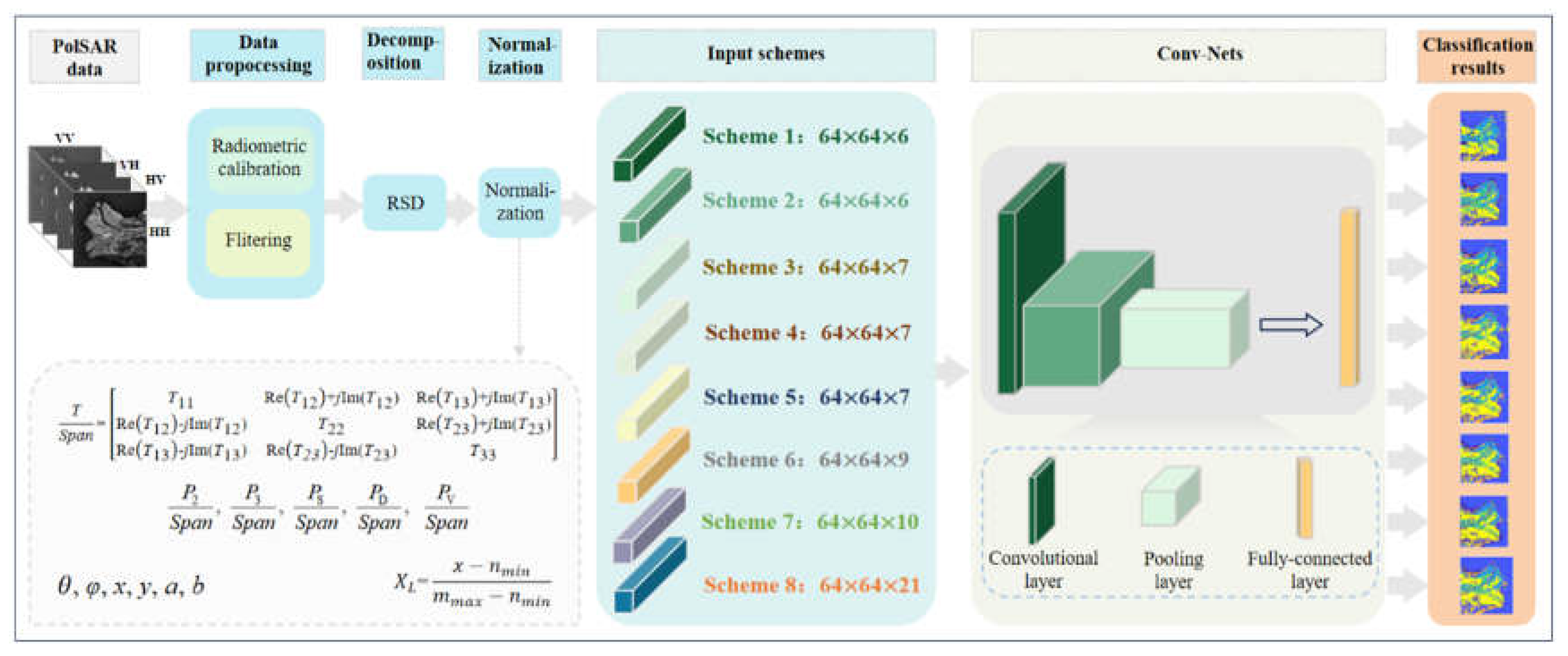
Figure 2.
Research area and ground truth map.
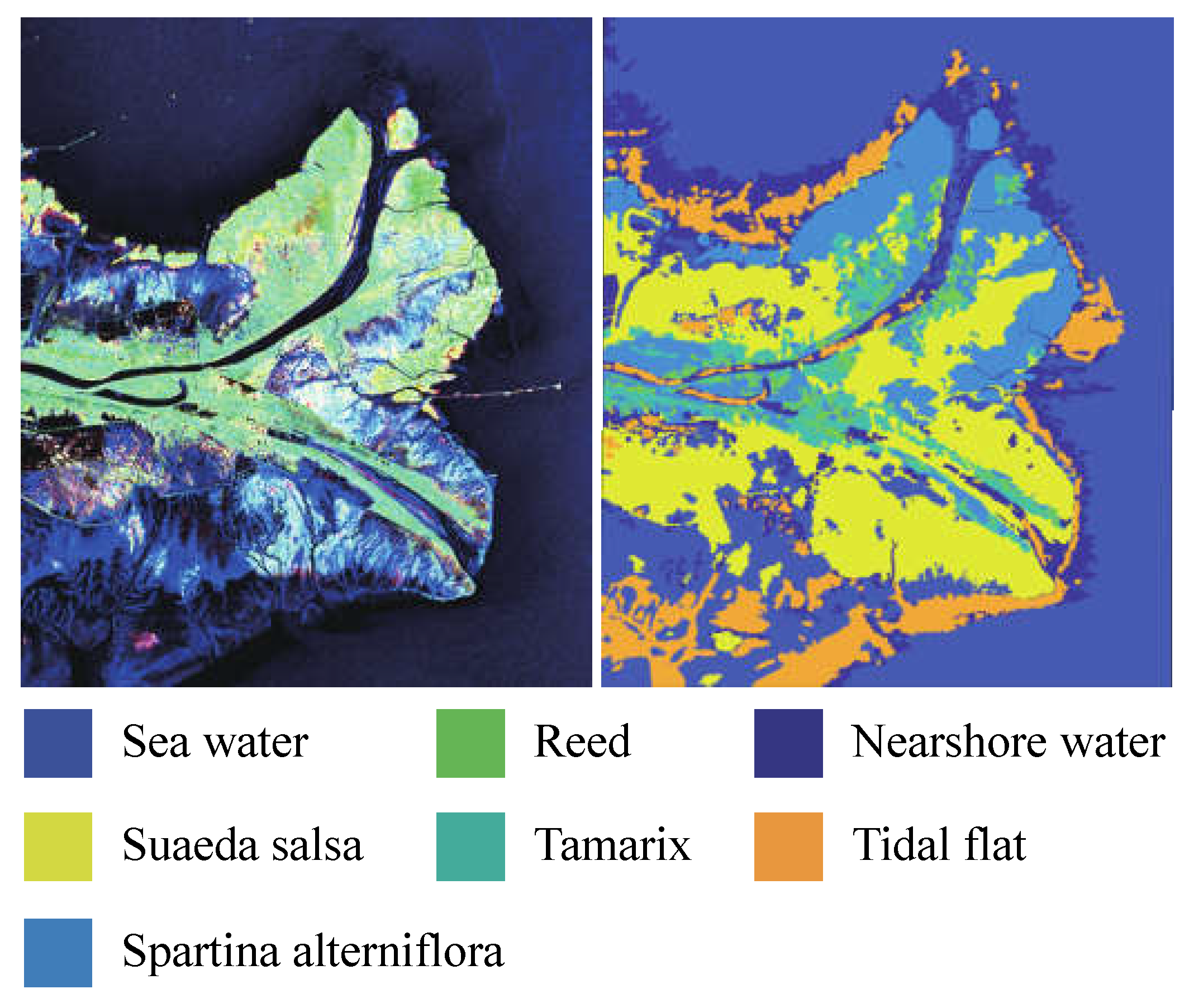
Figure 3.
Distribution of training, validation, and testing samples. (a) Image on September 14, 2021; (b) Image on September 14, 2021; (c) Image on October 13, 2021; (d) Image on October 12, 2017.
Figure 3.
Distribution of training, validation, and testing samples. (a) Image on September 14, 2021; (b) Image on September 14, 2021; (c) Image on October 13, 2021; (d) Image on October 12, 2017.
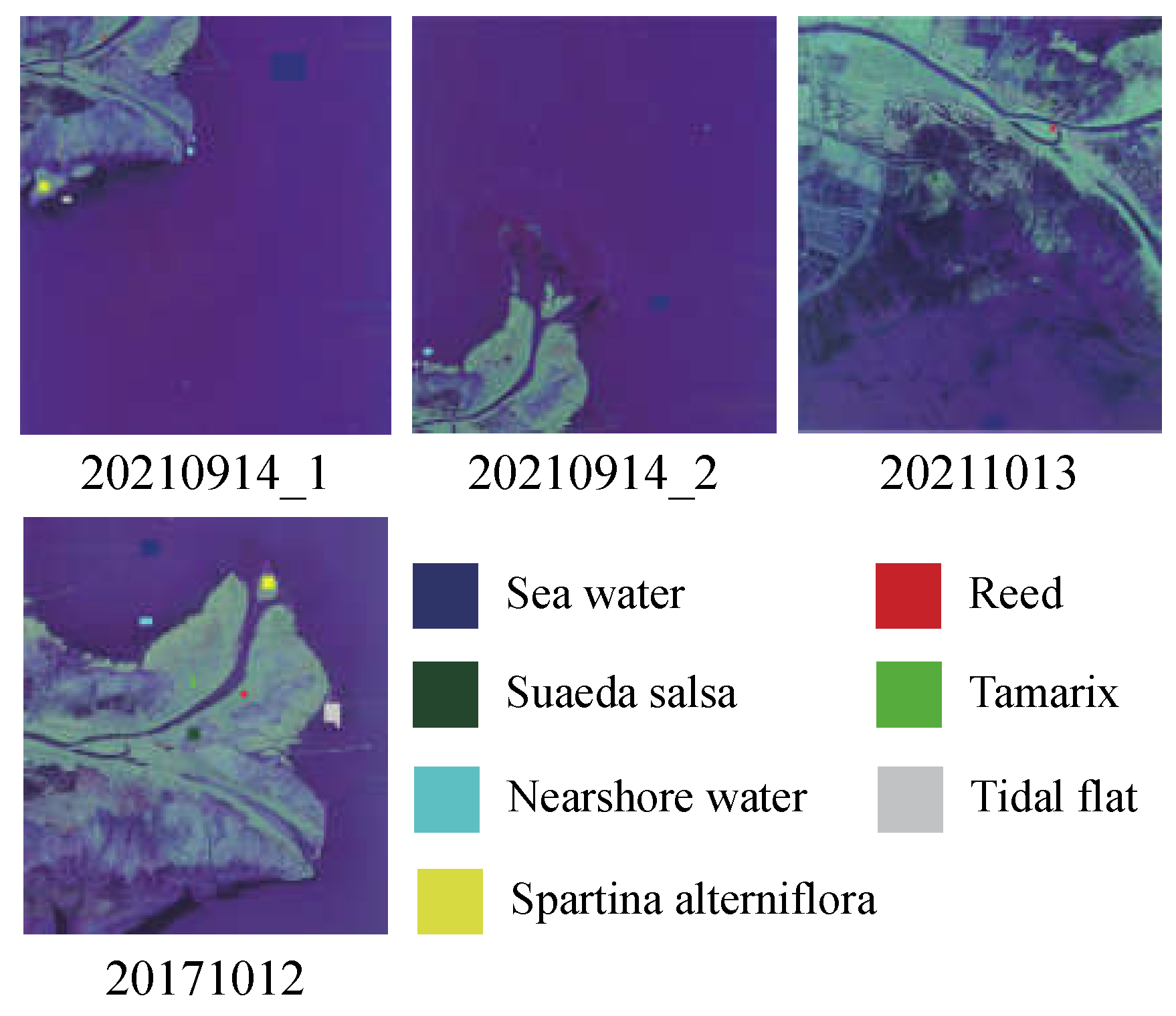
Figure 4.
Classification results of eight research schemes on AlexNet.
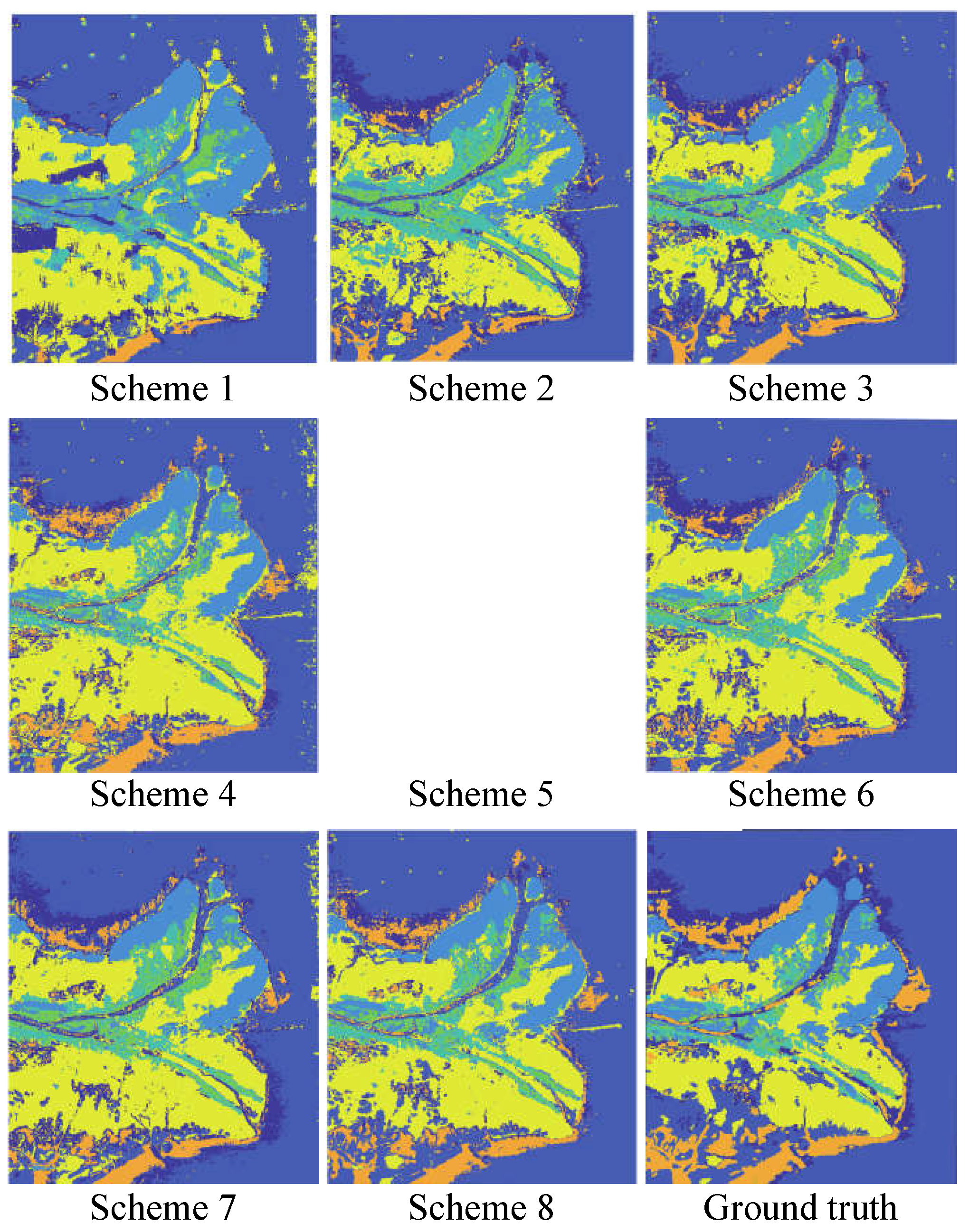
Figure 5.
Classification results of eight polarized data input schemes.
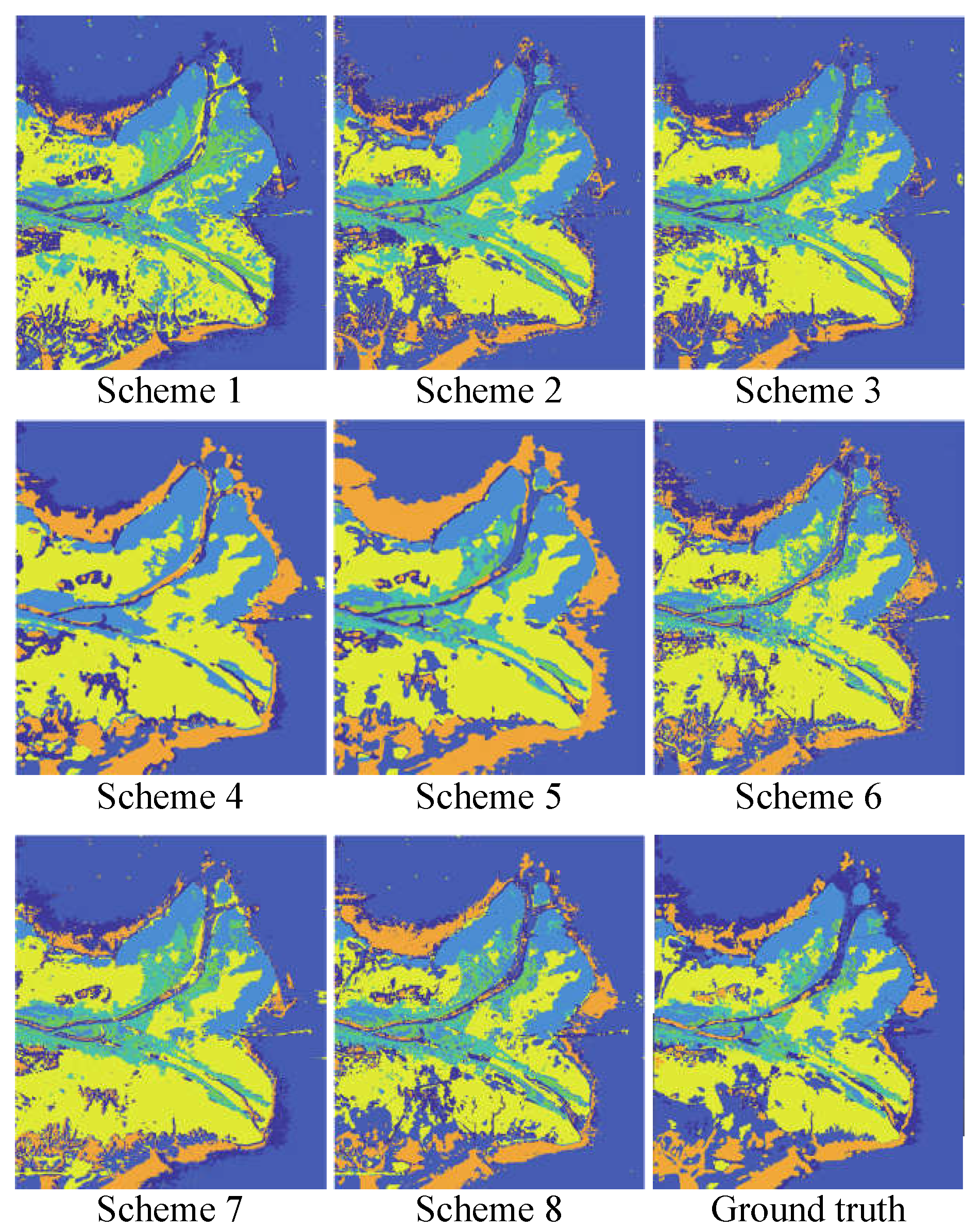
Figure 6.
Trend chart of overall classification accuracy and average accuracy.
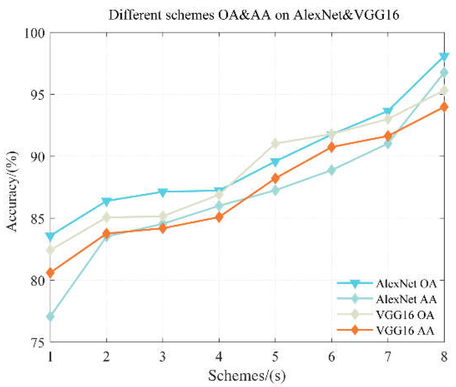

Table 1.
List of eight polarization data input schemes.
| Scheme | parameters | Polarization features |
|---|---|---|
| 1 | 6 | NonP0, T22, T33, coe12, coe13, coe23 |
| 2 | 6 | P0, T22, T33, coe12, coe13, coe23 |
| 3 | 7 | P0, T11, T22, T33, coe12, coe13、coe23 |
| 4 | 7 | P0,T11, T22, T33, PS, PD, PV |
| 5 | 7 | P0, T11, T22, T33, P2, P3, PV |
| 6 | 9 | P0, T11, T22, T33, P2, P3, PS, PD, PV |
| 7 | 10 | P0, T11, T22, T33, Re(T12), Re(T13), Re(T23), Im(T12), Im(T13), Im(T23) |
| 8 | 21 | P0, T11, T22, T33, Re(T12), Re(T13), Re(T23), Im(T12), Im(T13), Im(T23), P2, P3, PS, PD, PV, x, y, a, b |
Table 2.
Experiment images.
| Id | Date | Time (UTC) | Inc. angle (°) | Mode | Resolution | Use |
|---|---|---|---|---|---|---|
| 1 | 2021.09.14 | 22:14:11 | 30.98 | QPSI | 8 m | Train |
| 2 | 2021.09.14 | 22:14:06 | 30.97 | QPSI | 8 m | Train |
| 3 | 2021.10.13 | 10:05:35 | 37.71 | QPSI | 8 m | Train |
| 4 | 2017.10.12 | 22:07:36 | 36.89 | QPSI | 8 m | Test |
Table 3.
Distribution of Training and Validation Datasets.
| Images | Nearshore water | Seawater | Spartina alterniflora | Tamarix | Reed | Tidal flat | Suaeda salsa |
|---|---|---|---|---|---|---|---|
| 20210914_1 | 500 | 400 | 1000 | 500 | 500 | 500 | 500 |
| 20210914_2 | 500 | 200 | 0 | 0 | 0 | 500 | 0 |
| 20211013 | 0 | 400 | 0 | 500 | 500 | 0 | 500 |
| Total | 1000 | 1000 | 1000 | 1000 | 1000 | 1000 | 1000 |
Table 4.
Classification accuracy of the eight polarized data input schemes on the AlexNet network.
| Classification accuracy Input scheme |
1 | 2 | 3 | 4 | 5 | 6 | 7 | 8 |
|---|---|---|---|---|---|---|---|---|
| Nearshore water | 96.8 | 100 | 76.9 | 85.0 | 93.4 | 94.8 | 96.4 | 99.7 |
| Seawater | 96.9 | 100 | 99.5 | 98.8 | 98.7 | 99.2 | 98.7 | 99.7 |
| Spartina alterniflora | 96.8 | 100 | 93.3 | 93.2 | 85.2 | 92.9 | 95.5 | 100 |
| Tamarix | 100 | 97.6 | 99.0 | 93.8 | 75.9 | 100 | 96.0 | 96.7 |
| Reed | 94.5 | 98.3 | 93.4 | 63.7 | 93.3 | 94.9 | 99.2 | 100 |
| Tidal flat | 49.3 | 16.2 | 49.5 | 78.6 | 85.5 | 61.1 | 71.6 | 90.6 |
| Suaeda salsa | 50.8 | 92.7 | 98.4 | 97.6 | 95.1 | 99.4 | 98.2 | 100 |
| Indepent experiments Overall Accuracy | 83.59 | 86.40 | 87.14 | 87.24 | 89.59 | 91.76 | 93.66 | 98.10 |
| 81.41 | 85.19 | 84.27 | 87.19 | 88.91 | 91.76 | 91.84 | 96.54 | |
| 77.83 | 82.64 | 84.01 | 85.37 | 86.30 | 87.69 | 91.06 | 96.44 | |
| 73.66 | 81.86 | 83.67 | 85.29 | 86.19 | 86.61 | 89.29 | 96.40 | |
| 68.87 | 81.53 | 83.66 | 84.96 | 85.30 | 86.60 | 89.33 | 96.36 | |
| Average Overall Accuracy | 77.072 | 83.524 | 84.55 | 86.01 | 87.258 | 88.884 | 91.036 | 96.768 |
| Kappa coefficient | 0.8085 | 0.8413 | 0.8500 | 0.8512 | 0.8785 | 0.9038 | 0.9260 | 0.9778 |
Table 5.
Classification accuracy of eight polarimetric data input schemes on the VGG16 network.
| Classification accuracy Input scheme |
1 | 2 | 3 | 4 | 5 | 6 | 7 | 8 |
|---|---|---|---|---|---|---|---|---|
| Nearshore water | 95.7 | 82.5 | 91.1 | 91.3 | 94.9 | 93.4 | 90.5 | 77.2 |
| Seawater | 97.7 | 98.8 | 99.8 | 98.5 | 99.4 | 99.3 | 99.3 | 99.6 |
| Spartina alterniflora | 96.6 | 95.9 | 94.1 | 95.7 | 93.5 | 94.9 | 98.7 | 100 |
| Tamarix | 98.5 | 100 | 1000 | 67.5 | 100 | 89.6 | 99.9 | 90.8 |
| Reed | 93.8 | 85.0 | 91.3 | 68.0 | 82.2 | 69.6 | 91.7 | 99.9 |
| Tidal flat | 28.5 | 42.0 | 25.7 | 88.5 | 67.2 | 95.8 | 71.4 | 99.8 |
| Suaeda salsa | 66.2 | 91.3 | 94.1 | 98.9 | 100 | 100 | 99.6 | 100 |
| Indepent experiments Overall Accuracy | 82.43 | 85.07 | 85.16 | 86.91 | 91.03 | 91.80 | 93.01 | 95.33 |
| 82.21 | 85.03 | 84.66 | 86.63 | 88.99 | 90.61 | 92.03 | 94.93 | |
| 81.44 | 84.74 | 84.10 | 86.57 | 87.50 | 90.54 | 91.94 | 94.76 | |
| 79.44 | 82.06 | 83.64 | 84.90 | 86.77 | 90.43 | 91.29 | 92.96 | |
| 77.53 | 81.93 | 83.41 | 80.47 | 86.83 | 90.37 | 89.94 | 91.97 | |
| Average Overall Accuracy | 80.61 | 83.766 | 84.194 | 85.096 | 88.224 | 90.75 | 91.642 | 93.99 |
| Kappa coefficient | 0.7950 | 0.8258 | 0.8268 | 0.8473 | 0.8953 | 0.9043 | 0.9185 | 0.9455 |
Disclaimer/Publisher’s Note: The statements, opinions and data contained in all publications are solely those of the individual author(s) and contributor(s) and not of MDPI and/or the editor(s). MDPI and/or the editor(s) disclaim responsibility for any injury to people or property resulting from any ideas, methods, instructions or products referred to in the content. |
© 2024 by the authors. Licensee MDPI, Basel, Switzerland. This article is an open access article distributed under the terms and conditions of the Creative Commons Attribution (CC BY) license (http://creativecommons.org/licenses/by/4.0/).
Copyright: This open access article is published under a Creative Commons CC BY 4.0 license, which permit the free download, distribution, and reuse, provided that the author and preprint are cited in any reuse.


