
Submitted:
20 February 2025
Posted:
21 February 2025
You are already at the latest version
Abstract
Polarimetric Synthetic Aperture Radar (PolSAR) is an advanced remote sensing technology that provides rich polarimetric information. Deep learning methods have been proved an effective tool for PolSAR image classification. However, relying solely on source data input makes it challenging to effectively classify all land cover targets, especially heterogeneous targets with significant scattering variations, such as urban areas and forests. Besides, multiple features can provide more complementary information, while feature selection is crucial for classification. To address these issues, we propose a novel attention mechanism-based multi-feature lightweight deeplabV3+ network for PolSAR image classification. The proposed method integrates feature extraction, learning, selection, and classification into an end-to-end network framework. Initially, three kinds of complementary features are extracted to serve as inputs to the network, including polarimetric original data, statistical and scattering features, textural and contour features. Subsequently, a lightweight DeeplabV3+ network is designed to conduct multi-scale feature learning on the extracted multidimensional features. Finally, an attention mechanism-based feature selection module is integrated into the network model, adaptively learning weights for multi-scale features. This enhances discriminative features but suppresses redundant or confusing features. Experiments are conducted on five real PolSAR data sets, and experimental results demonstrate the proposed method can achieve more precise boundaries and smoother regions than the state-of-the-art algorithms.
Keywords:
Polarimetric SAR image classification
; Multi-feature extraction
; Lightweight DeeplabV3+ network
; Attention mechanism based feature fusion
1. Introduction
Polarimetric synthetic aperture radar (PolSAR) is an active microwave remote sensing detection technology, which is capable of obtaining multi-channel back-scattered echoes from the Earth’s surface. It possesses the capability of imaging in all weather and day-night. In comparison to Synthetic Aperture Radar (SAR) system [1], PolSAR system can capture a broader range of polarimetric characteristics and target scattering information, which has found widespread applications in various fields, including land cover classification [2], target identification [3], and ship detection [4] etc. The classification of PolSAR image is a crucial prerequisite in comprehending and interpreting PolSAR data, thus attracting increasing attention from researchers in the field of remote sensing.
Over the decades, numerous classification methods for PolSAR images have been proposed by researchers. The conventional approaches predominantly exploit shallow features to classify PolSAR images, which can be broadly categorized into three types. The first category involves statistical characteristic-based classification methods, notably including Wishart distribution [5], K distribution [6], as well as the Wishart mixture distribution model [7] etc. These methods are effective in modeling the statistical distribution of PolSAR data. The second category comprises classification methods based on target decomposition[8], such as Cloude decomposition [9], model-based polarimetric decomposition [10,11], polarimetric covariance eigenvalues[12], dominant scattering mechanism identification[13] and polarimetric roll-invariant features [14] etc. These methods utilize various scattering features to describe land covers from different views. In addition, machine learning approaches have been widely applied to PolSAR image classification. Widely adopted methods include the artificial neural network [15], support vector machine [16], and classification algorithms based on random forest[17]. These techniques aim to take advantages of potent polarimetric features for effective classification. However, these methods are limited to learning shallow characteristics. They encounter challenges in accurately classifying heterogeneous land covers due to the absence of high-level semantic features.
Recently, deep learning has witnessed rapid development in the realm of PolSAR image classification. In contrast to traditional methods, deep learning eliminates the need of manual selection of image features by autonomously extracting deeper features. Typical deep learning models include deep boltzmann machines [18], stacked auto-encoder [19], deep belief network [20], convolutional neural network (CNN) [21] and graph convolutional network [22], among others. To be specific, Zhang et al. [23] introduced a convolutional neural network with complex-valued coding (CV-CNN), enhancing feature extraction capability specifically tailored for PolSAR images. Guo et al. [24] presented an adaptive fuzzy super-pixel algorithm based on polarimetric scattering information for PolSAR image classification. In addition, Zhang et al. [25] introduced transfer learning and unsupervised deep learning networks to improve the classification results. Ai et al. [26] proposed a convolutional auto-encoder that incorporated textural feature fusion for land cover classification in PolSAR image.
With the evolution of deep learning models, various neural networks focusing on semantic segmentation have emerged successively. Notable networks in this domain include FCN [27], Unet [28], and DeepLab series (V1, V2, V3, V3+) [29,30,31,32]. Among them, the DeepLab series have achieved remarkable success in the field of semantic segmentation. Concurrently, in recent years, many PolSAR image classification algorithms based on the DeepLab series have been proposed. For instance, Zhang et al. [33] employed wavelet fusion and PCA dimensional reduction to suppress redundant features, combined with DeepLabV3 network for the classification of PolSAR images. In addition, Zhang et al. [34] incorporated the concept of SKNet units into DeepLabV3+, learning multi-scale polarimetric feature effectively, and thereby better applying to classification tasks. The DeepLabV3+ network[32] not only utilizes improved Xception network to integrate multi-dimensional information effectively, but also design spatial pyramid pooling (ASPP) module to learn multi-scale features. Therefore, DeepLabV3+ method can adaptive learn multi-scale features and semantic information, thereby exhibiting better performance for image classification. Here, we opt for the DeepLabv3+ network as the backbone network for PolSAR image classification. However, with too many parameters, DeepLabv3+ presents a complex network structure with a lot of time cost. To alleviate this problem, we design a lightweight DeepLabv3+ network tailored for PolSAR image classification, which can efficiently learn multi-scale semantic features for PolSAR image.
The aforementioned deep learning approaches empower the network to autonomously learn high-level features of targets, contributing to the enhanced accuracy of PolSAR image classification. However, these methods don’t fully exploit multiple scattering characteristics, which makes it challenging to effectively classify all land cover targets, particularly for heterogeneous ones such as urban areas and forests. It can be observed that significant scattering variations exists even within the interior of a heterogeneous ground object, making it difficult for the original data to categorize them into semantically consistent class. Actually, PolSAR data contain rich scattering features, target decomposition features, and texture features, which can provide complementary information for effective image classification [35,36]. For example, Wang et al. [37] introduced a PolSAR image classification method that jointly considered polarimetric features and adjacency information to gain classification advantage. Shi et al. [38] proposed a topic model for multi-feature joint learning, producing enhanced classification accuracy. Shang et al. [39] presented a CNN model based on spatial features, improving classification performance through a dual-branch network learning spatial features. Xu et al. [40] combined deep CNN with the Freeman-Durden decomposition algorithm to extract polarimetric features from PolSAR data, yielding more accurate result of building extraction. Wu et al. [41] employed a hybrid generative/discriminative network to learn the diversity of PolSAR echo statistical features and image spatial features, combined with variational Bayesian theory to integrate multiple features for PolSAR image classification. Collectively, these methods underscore the importance of leveraging multiple polarimetric features rather than relying solely on the original data.
However, existing deep learning classification methods have not fully exploited and utilized the diverse polarimetric information present in PolSAR images. In addition, it is widely acknowledged that an increased number of scattering features may not necessarily lead to better performance. Therefore, there are still two challenges for existing deep learning methods in PolSAR image classification. 1) How to maximize the utilization of the rich features embedded in PolSAR data to enhance the generalization and robustness of deep learning models. 2) How to adaptively select discriminative features from the multitude of available features, while simultaneously suppressing redundant or confusing features. Addressing these challenges is crucial for enhancing the overall classification performance of PolSAR images.
Fortunately, many feature selection methods have been proposed, such as correlation measurement [42], feature ensemble algorithm [43], dimensionality reduction [44], etc. Besides, the attention mechanism [45] has emerged as a widely used method for feature selection. It can automatically select interest regions and assign different weights for diverse regions, which has found extensive applications in target detection [46], image fusion [47] and classification [48]. However, it’s worth noting that these methods primarily operate on shallow feature selection, limiting their effectiveness in classifying complex terrain objects.
To alleviate these challenges, in this paper, we introduces a novel multi-feature lightweight deeplabV3+ network classification model, referred to as MLDnet. The model is an end-to-end deep network that integrates feature learning, feature selection, and classification together. Initially, we extract multiple scattering features from PolSAR images to provide a comprehensively representation of land cover information, encompassing original data, target decomposition features, textural and contour features. Subsequently, we design a lightweight L-DeeplabV3+ to train the network, facilitating the integration of multiple features and learning multi-scale high-level features, which significantly reduce network parameters. Additionally, an attention mechanism module is embedded after the L-DeeplabV3+ network. This module adaptively assigns weights to multidimensional features, enhancing relevant features for classification while suppressing redundant and confusing ones. Experimental results conducted on five real PolSAR data sets indicate that the proposed MFDAnet achieves higher classification accuracy compared to the state-of-the-art algorithms. The main contributions of the proposed MFDAnet method can be summarized into three key aspects.
- 1)
- A novel multi-feature deep attention network is proposed, which fully exploits diverse types of polarimetric features as the input, and automatically integrate the multi-feature learning, selection and classification into a unified framework. The multiple features include PolSAR original data, scattering features and image features, providing complementary information from different perspectives.
- 2)
- A lightweight DeeplabV3+ is developed as the backbone network of the MFDAnet. This architecture facilitates the learning of both multi-scale and multi-feature information, designing a lightweight scheme tailed for PolSAR images, ensuring a fast and effective network.
- 3)
- Attention mechanism-based feature selection module is embedded in the proposed MLDnet, adaptively learning weights of multi-dimensional features. This module enhances valuable features and suppresses redundant ones, thereby improving the classification performance.
2. Proposed Methodology
In this paper, a novel multi-feature deep attention network(MLDnet) is proposed for PolSAR image classification. It can learn multi-scale and multiple scattering features adaptively by designing a lightweight multi-feature DeeplabV3+ network. Additionally, it selects effective features using the attention mechanism, so as to finally realize the the effective classification of different land cover types.
The framework of our proposed multi-feature deep attention network is shown in Figure 1, comprising three key components: multi-feature extraction, lightweight DeeplabV3+ network design and attention-based feature fusion and classification. Firstly, in contrast to traditional network using 9-dimension PolSAR data as the input, we extract multiple scattering features as the network input. They include original data, scattering mechanism-based and image analysis-based features, fostering enhanced information complement; Secondly, we design a lightweight DeeplabV3+ network to automatically learn features of different scales from multiple features; Finally, the multi-scale multi-features are automatically selected by the channel attention module embedded in the network. This process enhances valuable discriminating features with larger weights while disregarding useless features with smaller weights. The classification layer is then employed to determine the probability of the target, yielding the final classification result. Further details are introduced as follows.
2.1. Multi-Feature Extraction Module
Traditional CNN model usually converts the PolSAR covariance matrix into a 9-dimension real vector as the network input, creating a cube with 9 channels for each pixel. However, 9-dimension vector is not adequate to represent the complexity of PolSAR image for each pixel. Additional information, such as scattering characteristics [49][50], has been proved effective for identifying ground objects. Moreover, the contextual features, including textural and contour features, play a significant role in describing image contextual information. Numerous studies highlight the value of multiple features in enhancing classification performance. Therefore, we propose a multi-feature data representation as the network input. Before multi-feature extraction, a refined Lee filter[51] is applied to the original PolSAR image. Compare with other advanced filter methods[52,53], the refined Lee filter is a classical filtering method to reduce speckle noises fastly and effectively, which can be easily conducted upon the PolSARPro software. Specifically, three types of features are extracted to formulate a 57-dimensional feature vector as PolSAR data expression, which is extracted from PolSAR original data, target decomposition features, as well as textural and contour features respectively. The detailed feature extraction procedure is outlined below.
1)PolSAR original data (16-dimension): It consists of scattering matrix , coherency matrix and SPAN image. The original PolSAR data is scattering matrix , defined as :
After multi-look processing, the most commonly used coherency matrix is derived by Equation (2), which is shown on the top of the next page.
In Equation (2), * represents the complex conjugate operation. Since the complex matrix cannot be fed to the network directly, similar to other networks, we convert the coherency matrix to a 9-dimension vector, defined as
where is the real part of , and is the imaginary part of . In addition, the Polarimetric-Total-Power (SPAN) value is the power image, which is calculated by summarizing the diagonal elements of matrix, defined by
2)Target decomposition-based features (17-dimension): It contains three target decomposition-based parameters and two polarimetric parameters, which can describe target’s scattering mechanism from various perspectives. Three types of target decompositions are Cloude and Pottier decomposition [54], Freeman decomposition [55] and Huynen decomposition [56]. These decomposition methods have been proven effective for PolSAR image classification, serving as valuable features for distinguishing different ground objects. Furthermore, the two polarimetric parameters are the co-polarization ratio [57] and the cross-polarization ratio [58]. The former is used to measure the difference between and , and the latter is highly sensitive to volume scattering. All these scattering features represent independent attributes of each resolution unit, providing distinct descriptions for each pixel.
3)Image features (24-dimension): In addition to the original data and scattering features, each pixel, acting as a unique scattering unit, also has a close relationship with neighborhoods to formulate a PolSAR image, that is contextual features such as texture and contour. These features play a crucial role in identifying the ground objects. To capture the contextual relationship, we extract GLCM features [59], a widely used technique for textual feature extraction in natural images. It encompasses four types of features, including contrast, energy, entropy and relativity. Additionally, we extract the edge and line energies using filters with 18 directions and 4 scales, providing information on the contour and strength of image edges. All 57-dimension features are summarized into Table 1.
2.2. Lightweight DeepLabV3+ Network
The DeepLab series [29,30,31,32], a collection of semantic segmentation algorithms developed by the Google team, has demonstrated notable advancements in semantic learning. Leveraging depth-wise separable convolution technology, DeeplabV3+ efficiently integrates features in the depth direction, requiring fewer parameters. In addition, the DeepLabV3+ network introduces the Atrous Spatial Pyramid Pooling (ASPP) technique to integrate multi-scale information. This technique utilizes convolution layers with different dilation factors, increasing the receptive field and reducing information loss during down sampling. Therefore, we select the DeeplabV3+ network as the backbone of the proposed method, since it can integrate multi-dimensional features and learn multi-scale semantic information effectively.
However, the original backbone network used by DeeplabV3+ network is an improved Xception network, as depicted in Figure 2, featuring a complex network structure. Furthermore, in semantic segmentation tasks, the input unit is typically an image, while for PolSAR image classification, the input unit is a small image block, with a smaller input feature block and a larger data amount. So, considering these differences between semantic segmentation and pixel-wise classification, a revised DeeplabV3+ network should be tailored for PolSAR image classification.
In this paper, we develop a lightweight DeeplabV3+ network, named L-DeeplabV3+, as an alternative. Taking a PolSAR image with pixels as an example, Table 2 provides the comparison of network parameters between the L-DeeplabV3+ network used in this article and the original DeeplabV3+network. In addition, Figure 3 also illustrates the structure differences between the proposed L-DeeplabV3+ and original DeeplabV3+ networks, which can be summarized into three key aspects.
1)Input: First of all, as mentioned earlier, the whole image serves as the network input in the semantic segmentation task in Figure 3(a). However, for PolSAR image classification task, the input image block is sampled by a square window centered on each pixel, as shown in Figure 3(b). It also can be found in Table 2 that the size of the input feature map are (image size) and (window size) for DeeplabV3+ and L-DeeplabV3+ networks respectively.
2)Backbone network: For the backbone network, the DeeplabV3+ network employs an improved Xception network, as shown in Figure 2, adept at handling larger input features. However, it may lead to overfitting when dealing with small input blocks. As depicted in Table 2, the proposed L-DeeplabV3+ network adopts two convolutional layers as the backbone network. This design allows for the extraction of shallow features without significantly reducing the feature dimension. In addition, we introduce a max-pooling layer between the two convolutional layers to further reduce the number of model parameters and mitigate the risk of model overfitting.
3)Multi-scale feature learning: In addition, as is well known, with the increasing dilated rate, the receptive field will also become larger. Therefore, in the original DeeplabV3+, a relatively large dilation rate is set to achieve the segmentation of large objects. However, for a PolSAR image block, an excessively large dilation rate can lead to the loss of local detailed information, thereby affecting the final classification results. In L-DeeplabV3+, we address this issue by significantly reducing the dilation rate in the ASPP module. This adjustment allows the network to capture multi-scale contextual information while preserving local detailed information. The detailed parameter comparison can be seen in Table 2.
In summary, the proposed multi-feature-based L-DeeplabV3+ network achieves multi-scale feature learning for the multi-dimensional features of PolSAR images. This is accomplished while maintaining the original DeeplabV3+ network framework and further reducing network parameters and unnecessary time overhead.
2.3. Attention-Based Multi-Feature Fusion and Classification
After processing through L-DeeplabV3+ network, we attain multi-scale multi-feature information in channel dimension, which can provide rich contextual features for classification. However, recognizing that not all scattering features contribute equally to classification, the selective extraction of valuable features while suppressing less relevant ones remains a challenging issue. In this paper, we propose an attention-based multi-feature fusion module to ensemble with the L-deeplabV3+ network. This module dynamically learns different weights for diverse scattering features in channel direction, highlighting important features and diminishing less useful ones. Ultimately, we achieve multi-scale multi-feature fusion in both spatial and channel dimensions.
The attention-based multi-feature fusion module, illustrated in Figure 4, begins by separately aggregating multi-scale spatial features through max-pooling and average-pooling layers. This process generates two distinct feature maps, each encapsulating spatial contextual information. Subsequently, these two feature maps are input to a shared fully connection layer, producing their respective channel attention feature maps. The next step involves summing these two attention feature maps, followed by the application of an activation function. This results in the aggregation of their information, ultimately yielding channel attention weights.
Assuming that the size of the output feature map X by L-deeplabV3+ network is , the obtained channel attention weight is W, with the size of , through the attention mechanism. The procedure of the channel attention module can be described as:
where X is the learned feature map from L-DeeplabV3+, and are the parameters of two fully connecting layers and is the non-linear translation. and are average and max pooling layers respectively. is the activation function.
The feature map X is then multiplied by the weight W to obtain the channel attention fusion features, defined as:
where ⊗ represents multiplying each channel feature with the obtained weight one by one. After obtained the fused feature F, a classifier is applied to achieve the final classification map.
The whole algorithm procedure of the proposed MLDnet is given in Algorithm 1. The algorithm begins by applying the refined Lee filter to mitigate speckle noise. Subsequently, multiple features are extracted from PolSAR images, including original PolSAR data, target decomposition features, textual and contour features. These multi-features are then input into the L-DeeplabV3+ network to learn the multi-scale high-level features. Furthermore, an attention mechanism is applied to the multi-scale features, enabling the automatic selection and fusion of multiple features by learning different weights. This ensures that valuable features are assigned larger weights while redundant features receive smaller weights. Finally, the output of the MLDnet passes through a classifier to obtain the final classification result.
| Algorithm 1 Procedure of the proposed MLDnet method |
| Input:PolSAR original data , PolSAR original image , class label map and class number . |
| Step 1: Apply a refined Lee filter to PolSAR original image to obtain the filtered PolSAR image . |
| Step 2: Extract 57-dimensional features F from PolSAR image and PolSAR original data based on Table 1. |
| Step 3: Using a fixed-size square window to sample the extracted 57-dimensional features F pixel by pixel, obtaining N data with a shape of , where N is the total number of image pixels. |
| Step 4: According to a certain ratio, the N data obtained in step 3 and the label map L are divided into training set and test set . |
| Step 5: Import the training set into the MLDnet network for training until reaching the iteration number, saving the training model, training loss, and model parameters. |
| Step 6: Using the trained model to predict and classify the test set . |
| Output: class label estimation map and various evaluation indicators. |
3. Experimental Results and Analysis
3.1. Experimental Data and Settings
In order to verify classification performance of the proposed MLDnet, extensive experiments are conducted on five real PolSAR data sets. These data sets cover Xi’an, Oberpfaffenhofen, San Francisco and Flevoland areas respectively. Detailed information is given as follows:
A)Xi’an data set: The first data set is C-band full polarimetric SAR data collected from Xi’an in the western region of China using RADARSAT-2 system. The image size is pixels, with a resolution of meters. It encompasses three types of land cover classes: building, grass, and water. The Pauli-RGB pseudo-color image and the corresponding ground truth image are presented in Figure 5(a).
B)Oberpfaffenhofen data set: The second data set covers the Oberpfaffenhofen area in German and consists of an 8-look L-band fully PolSAR image acquired by the E-SAR sensor at the German Aerospace Center. This polarimetric radar image has the dimension of pixels with a resolution of m. It includes five distinct land cover types: bare ground, forest, farmland, road and building. Figure 5(b) illustrates the Pauli RGB image of the Oberpfaffenhofen data set along with the corresponding ground truth map.
C)San Francisco data set: The third data set is the San Francisco data set, which is a C-band fully PolSAR image collected by the RADARSAT-2 system over the San Francisco area in the United States. The image has a resolution of m and a size of pixels. Its Pauli RGB image and ground truth map are displayed in Figure 5(c), which contains five different land cover types: ocean, vegetation, low density urban, high density urban, and developed.
D)Flevoland1 data set: The fourth data set is C-band fully polarimetric SAR data collected by the RADARSET-2 sensor in the Flevoland region of the Netherlands. The image size is pixels, with a resolution of m. The PolSAR image encompasses four types of land cover, including water, urban, woodland, and cropland. We name this data set the Flevoland1 data set. Figure 5(d) exhibits the Pauli-RGB image along with the corresponding ground truth map of the Flevoland1 data set.
E)Flevoland2 data set: The last data set comes from the Flevoland region and consists of full-polarization L-band SAR data acquired by the AIRSAR system. The spatial resolution is m, and the image size is pixels. The Pauli RGB image and its ground truth are shown in Figure 5(e). This image includes 15 types of crops: stem beans, peas, forest, lucerne, beets, wheat, potatoes, bare soil, grasses, rapeseed, barley, wheat2, wheat3, water and buildings. We name it the Flevoland2 data set.
The quantitative metrics employed in our experiments include average accuracy (AA), overall accuracy (OA), and Kappa coefficient. Experiments are conducted on Windows 10 operating system, using a 64GB NVIDIA GeForce GTX 3070 PC. The algorithm is implemented with Python 3.7 and Pytorch GPU 1.9.0. In addition, we utilize the Adam optimizer with a learning rate of 0.0001. The batch size is defined as , and the number of training iteration is 50. The multi-class cross-entropy loss is employed. During the experimental process, 10% of the training samples are selected for each class of land cover in the image, with the remaining 90% serving as test samples. It should be noted that the white regions in the ground truth maps are unlabeled pixels in Figure 5 and ??. During classification, all pixels in PolSAR images can obtain classification result, while unlabeled pixels are not considered into calculating quantitative metrics. Therefore, we just give the classification map with labeled pixels, and unlabeled pixels are colored by white in the following experimental results.
To assess the effectiveness of the proposed MLDnet, we compare it with seven state-of-the-art classification algorithms: Super-RF [17], CNN [21], CV-CNN [23], 3D-CNN [60], PolMPCNN [61], CEGCN [62] and SGCN-CNN[63]. Specifically, the first compared method combines the random forest algorithm with superpixels, utilizing G0 statistical texture features to mitigate the interference from background targets, such as forests, on farmland classification, referred to as Super-RF. The second method, referred to as CNN, converts PolSAR data into normalized 9-D real feature vectors and learns hierarchical polarimetric spatial features automatically through two cascaded convolutional layers. The third method is a complex-valued convolutional neural network, named by CV-CNN. This approach transforms the PolSAR complex matrix into a complex vector, effectively leveraging both the amplitude and phase information presented in PolSAR images. The fourth method is based on 3-D convolutional neural network, shorted by 3D-CNN. It utilizes 3-D CNN to extract deep channel-spatial combined features, adapting well to the 3D data structure for classification. The fifth method combines polarimetric rotation kernels, employs a multi-path structure and dual-scale sampling to adaptively learn the polarimetric rotation angles of different land cover types, noted by PolMPCNN. The sixth method employs a graph encoder and decoder to facilitate collaboration between CNN and GCN within a single network, shorted by CEGCN. It enables feature learning in small-scale regular and large-scale irregular regions, respectively. The last approach similarly integrates super-pixel level and pixel-level networks into a single framework, named SGCN-CNN for short. It can obtain both global features and local features by defining the correlation matrix for feature transformation between superpixel and pixel.
3.2. Experimental Results on Xi’an Data Set
Classification results on the Xi’an data set are displayed in Figure 6(b)-(i), illustrating the classification maps generated by Super-RF, CNN, CV-CNN, 3D-CNN, PolMPCNN, CEGCN, SGCN-CNN and the proposed MLDnet methods, respectively. Specifically, Figure 6(b) displays the output of the Super-RF method, revealing numerous misclassified pixels, primarily concentrated around the water class. At the same time, these misclassifications form distributed blocks due to superpixels. In contrast, the CNN method performs exceptionally well in distinguishing the water class, but exhibits misclassifications in the building class due to the lack of global information. It erroneously classifies some building as grass class. Similar to the CNN method, the CV-CNN exhibits noticeable misclassifications in the building and grass classes due to pixel-wise local features. 3D-CNN can adapt to the 3D structure of input data for classification, thus achieving better regional consistency. However, it struggles to adaptively handle distinct individual features, limiting its classification effectiveness at the boundaries of different land covers. In comparison, PolMPCNN excels in adaptively learning the polarimetric characteristics of various land covers, greatly improving overall classification effect. However, the feature learning procedures of different terrains are independent, resulting in a small number of misclassified pixels still existing at the land covers boundaries. Compared to PolMPCNN, the CEGCN method utilizes two branches, CNN and GCN, to generate complementary contextual features at the pixel and super-pixel levels, significantly improving classification accuracy at boundaries of diverse land covers. However, the CEGCN method cannot handle the inherent speckle noise in PolSAR images well, so there are some noise points in the image. The SGCN-CNN method, similar to the CEGCN method, also struggles to effectively handle the inherent speckle noise in images, resulting in the generation of a significant number of noise points. The proposed MLDnet combines the L-DeeplabV3+ network to deeply explore multi-dimensional features of PolSAR image, and select effective features through the incorporation of a channel attention module. Compared to six contrastive methods, the proposed MLDnet method in (h) demonstrates substantial improvements in both regional consistency and edge details.
Table 3 lists the classification accuracy of all methods in the Xi’an data set. It can be seen that the Super-RF method without deep features has lower accuracy than other methods. The main reason is that the classification accuracy of water class is only 70.91%, which is relatively consistent with the classification result in Figure 6(b). In comparison, CNN has greatly improved its accuracy in water class, but its accuracy in the building class is relatively lower, resulting in the low overall accuracy. It only improved by 0.27% compared to Super-RF. CV-CNN further improves the classification accuracy of the water class, with the highest accuracy among all methods. However, its classification accuracy in the grass class is the lowest among all methods, which also results in its OA value being slightly lower than CNN. Compared to the previous three methods, 3D-CNN has achieved a significant improvement in OA value, and PolMPCNN has further improve the performance, especially in the building class, with the accuracy of 97.68%, which is significant higher than other compared methods. Analogously, due to better distinguishing grass class, CEGCN has further improved the overall classification accuracy. The SGCN-CNN method experiences a decline in overall classification metrics due to a significant number of misclassifications within grass class. The proposed MLDnet achieves the best classification accuracy in both two land cover types and three overall evaluation indicators. Specifically, the OA values are improved by 7.44%, 7.17%, 7.79%, 4.17%, 3.37%, 1.17% and 6.20% compared to other methods.
Figure 7 shows the confusion matrix of the Xi’an data set. From the figure, it can be seen that the proposed method misclassifies 2030 (about 5.70%) pixels of water class as grass, while misclassifying 1654 (about 1.40%) pixels of grass as water class. In addition, there are also a small number of misclassified pixels in the building class, with 1385 pixels (about 1.65%) misclassified as grass.
3.3. Experimental Results on Oberpfaffenhofen Data Set
The classification maps produced by compared and proposed methods are illustrated in Figure 8(b)-(i), respectively. As shown in Figure 8(b), the Super-RF method effectively distinguishes bare ground and farmland classes due to large number of samples. However, for classes with fewer samples such as building, forest, and road classes, misclassification is more noticeable. The CNN method shown in (c) has enhanced classification performance for building and road classes. However, its effectiveness in differentiating the farmland class remains suboptimal. In comparison, the CV-CNN method in (d) shows a marginal improvement in mitigating misclassification issues related to the farmland class. Nevertheless, it exacerbates misclassification in the bare ground class in the upper left corner, and overall regional consistency remains relatively poor. The 3D-CNN method in (e) exhibits similar to the Super-RF method, displaying a notable number of misclassified pixels in the road and farmland classes. Despite this, there is an enhancement in building class. Compared to the preceding four methods, the PolMPCNN method in (f) demonstrates a substantial improvement in regional consistency. However, this method almost entirely misclassifies the road class in the lower half of the images as the building class. Additionally, the boundaries between different land covers appear blurry. CEGCN has further enhanced the classification performance of the road class, building upon the foundation laid by PolMPCNN. However, the effectiveness is still suboptimal. The SGCN-CNN method in (h) likewise demonstrates subpar performance when dealing with classes with fewer samples, such as road and farmland. The proposed MLDnet method, as exhibited in (i), demonstrates a remarkable improvement in the classification performance of all five land covers compared to other contrastive methods. Furthermore, it effectively preserves the boundaries among different land covers.
Table 4 compares the classification accuracy of different methods in the Oberpfaffenhofen area. From the table, it can be visually observed that the seven compared methods have relatively low OA values on the Oberpfaffenhofen data set, with the highest value being only 88.93% (CEGCN). Moreover, among the five land cover types, bare ground class exhibits relatively high accuracy in discrimination. The four comparative methods (Super-RF, 3D-CNN, CEGCN and SGCN-CNN) all achieve accuracy rates exceeding 90%. Meanwhile, all seven comparative methods have an accuracy rate surpassing 81% for forest class. However, for the remaining three classes, particularly farmland and road classes, none of the seven comparative methods achieve satisfactory performance. The highest discrimination rates are 80.70% (CEGCN) for farmland class and 76.20% (CVCNN) for road class. Notably, for the road class in PolMPCNN, the correct discrimination rate is only 10.38%, consistent with the classification result displayed in Figure 8(f). This indicates that for data sets with unbalanced samples, such as Oberpfaffenhofen, the classification performance of the six comparison methods is constrained. However, The proposed MLDnet method excels in achieving the highest classification accuracy across all evaluation metrics, with values consistently exceeding 93%. Furthermore, in comparison to the seven comparative algorithms, the OA value sees an increase of 17.79%, 15.32%, 21.31%, 13.37%, 20.37% ,7.26% and 18.90%, respectively. This highlights the superior capability of the proposed method in effectively handling complex scenes of PolSAR images and enhancing classification accuracy.
Additionally, the confusion matrix of the Oberpfaffenhofen data set is depicted in Figure 9. The figure reveals that, for the bare ground class, the primary misclassification occurs in the road class, comprising 9437 pixels (approximately 1.23%). Regarding the forest class, it is primary misclassified as the bare ground class, accounting for 6277 pixels (approximately 2.33%). Similarly, for the building, farmland, and road classes, they are primarily misclassified as the bare ground class, with 4024 pixels (approximately 1.63%), 2038 pixels (approximately 2.04%), and 10572 pixels (approximately 5.89%), respectively. Therefore, the main confusion appears between bare ground and road classes.
3.4. Experimental Results on San Francisco Data Set
The experimental results of seven contrastive methods and MLDnet algorithms on the San Francisco data set can be seen in Figure 10(b)-(i), respectively. Figure 10(a) displays the ground truth map of the San Francisco area. Upon comparing the ground truth map, it is evident that super-RF produces many misclassifications in high density urban class with significant surface scattering differences. It also exhibits a portion of confusion between vegetation and developed classes. The CNN method also faces challenges in distinguishing high density urban class from developed class. In comparison to the previous two methods, the classification performance of CV-CNN has been improved in high density urban and developed classes, while there are still a small number of misclassified pixels. Simultaneously, the misclassification phenomenon in low density urban class is also quite evident. The 3D-CNN method demonstrates improved classification performance on high-density urban, low-density urban, and developed classes but exhibits more misclassified pixels in the vegetation class. PolMPCNN improves classification performance in various classes. However, its classification map still contains some visually apparent misclassified pixels. CEGCN and SGCN-CNN almost perfectly distinguish various land covers; however, upon closer observation, it is not difficult to notice that they have some misclassified pixels along land cover boundaries. The proposed MLDnet method also effectively distinguishes various land covers, meanwhile, it preserves the boundaries of different land cover types well. This suggests that the MLDnet method is effective in achieving good classification results even for large-scale PolSAR data sets.
In addition, Table 5 provides the classification accuracy of all methods for various land covers in the San Francisco data set, along with the corresponding OA, AA, and Kappa. Based on the table, it can be observed that, in comparison to the other three land cover types, both the Super-RF and CNN methods exhibit relatively low accuracy in classifying high density urban and developed classes. This is especially evident for the Super-RF method, with precision rates of 77.76% and 81.00%, respectively. CV-CNN exhibits a relatively low accuracy rate in the low density urban class. In comparison, the classification accuracy by 3D-CNN and PolMPCNN methods is higher, with OA values both above 98%. The CEGCN and SGCN-CNN methods both exhibit excellent performance across five different land cover types, with accuracy exceeding 99% for all categories except vegetation class. In contrast, the proposed MLDnet method achieves the highest class accuracy for all five land cover types, demonstrating superior classification performance. In terms of overall metrics, using OA metric as an example, compared to the seven other comparative algorithms, MLDnet improves OA by 5.64%, 3.69%, 2.26%, 1.59%, 1.04%, 0.42%, and 0.50% respectively.
The confusion matrix of the MLDnet applies on the San Francisco data set is presented in Figure 11. From the figure, it can be observed that MLDnet achieves the best discrimination between ocean and developed classes, with the main misclassification occurring in the vegetation class, consistent with the results shown in Table 5.
3.5. Experimental Results on Flevoland1 Data Set
The experimental results of various methods on the Flevoland1 data set in the Netherlands are depicted in Figure 12. Specifically, the Super_RF in (b) is a low-level feature learning method that exhibits limitation in effectively classifying urban class. In contrast, the CNN method in (c) demonstrates some enhancement in the classification of land cover boundaries; however, the overall classification performance remains inadequate, marked by numerous noisy points in the image. The CV-CNN method in (d) and the 3D-CNN method in (e) have enhanced regional consistency to some extent, but the improvement effect is not significant. There are still relatively noticeable misclassification pixels in the classification maps. PolMPCNN in (f) further enhances the regional consistency, effectively distinguishing between water and woodland classes, with only a small amount of misclassified pixels in cropland and urban classes. CEGCN in (g) and SGCN-CNN in (h) further enhance the ability to distinguish various land cover types, with only a few misclassifications occurring at the boundary between cropland and urban classes. The proposed MLDnet in (i), leveraging a 57-dimensional multi-feature and the L-DeeplabV3+ deep learning network, exhibits a notable improvement compared to previous methods. There are almost no obvious misclassification phenomena in the image. The consistency of regions and the preservation of boundaries have been significantly enhanced.
In addition, to quantitatively assess the classification performance, the classification accuracies of all methods on the Flevoland1 data set are presented in Table 6. It is evident that Super-RF attains the lowest correct classification rate of 81.84% in the urban class. CNN method achieves the lowest classification accuracy in the cropland class, at 93.16%. CV-CNN demonstrates great improvements, especially for the water class, with a correct discrimination rate second only to the proposed method MLDnet, reaching 99.85%. 3D-CNN method improves the classification accuracy in the cropland class compared to the previous three methods, with increases of 2.59%, 3.59%, and 2.81% respectively. PolMPCNN method further improves the classification metrics for various classes in the Flevoland1 data set, achieving an OA value of 98.49%. The CEGCN and SGCN-CNN further improve the classification accuracy of various types of land cover, with numerical values consistently above 98%. Additionally, it is noticeable that multiple comparison algorithms exhibit relatively lower correct classification rates for the urban class. This suggests that the classification of the urban class is more difficult. However, it is obvious that the proposed MLDnet excels in classifying all types of land covers and in overall classification performance. Especially for the urban class, the accuracy has also reached 99.98%. This demonstrates the effectiveness of the proposed method.
The confusion matrix of the Flevoland1 region is depicted in Figure 13. It is evident that in the differentiation of four different land covers, the number of misclassified pixels is relatively low using the proposed MLDnet. Especially in the water class, the number of misclassified pixels is only 10, while the total number of pixels in the water class in the Flevoland1 data set is 256369.
3.6. Experimental Results on Flevoland2 Data Set
The experimental results using the proposed MLDnet method and seven comparison methods on the Flevoland2 data set are shown in Figure 14. By comparing these results with the label map in (a), it is evident that the superpixel-level classification method, Super-RF, and the pixel-level classification method, CNN, exhibit numerous patchy misclassified areas and scattered misclassification noise across multiple classes. In contrast, the CV-CNN method achieves better classification results, though it still shows noticeable misclassified pixels in the rapeseed class. Furthermore, due to the lack of global information, the 3D-CNN method generates spotty noise in multiple classes such as stem beans, wheat, and rapeseed. PolMPCNN effectively learns various land cover features through a multi-path architecture but still has limitations in distinguishing similar land covers such as barley, wheat2, wheat3, and rapeseed. CEGCN combines pixel-level and superpixel-level features effectively, resulting in good differentiation of various land covers, with only a few misclassifications in the rapeseed and wheat classes. The SGCN-CNN method exhibits a small number of misclassifications in the wheat2, rapeseed, and grasses classes. Additionally, the analysis reveals that all seven comparison methods exhibit varying degrees of misclassified pixels in the rapeseed class. However, the proposed MLDnet method achieves excellent classification performance across all land covers, including the rapeseed class. This success is contributed to the proposed MLDnet method, which comprehensively considers different land cover characteristics and extracts various features such as texture and contour features, thereby enhancing the network’s ability to distinguish similar crops.
Meanwhile, Table 7 provides the per-class accuracy, overall accuracy (OA), average accuracy (AA), and Kappa coefficient for the above methods and the proposed model. The data show that the Super-RF method achieves excellent classification performance in the barley and water classes, with an accuracy of 100%, but completely misclassified the buildings class, thus lowering the average accuracy. The CNN method shows a slight improvement in OA, but not reach 90% accuracy in several classes, such as grasses and barley. In contrast, CV-CNN significantly improves both class differentiation and overall evaluation metrics, achieving an OA of 98.96%. Similar to Super-RF, 3D-CNN performs well in the water class but fails in buildings class. PolMPCNN, on the other hand, differentiates the buildings class well but has the lowest class accuracy in the barley class, with only 40.25%. CEGCN achieves over 99% class accuracy in multiple classes, with main misclassifications occurring in the peas, grasses, and buildings classes. The SGCN-CNN method shows a slight improvement over CEGCN, with all metrics exceeding 90%. However, the proposed MLDnet achieves the highest class accuracy in all 13 land cover types, with an overall accuracy of 99.95%. These results fully validate the effectiveness and reliability of the proposed method.
The confusion matrix of the Flevoland2 region is presented in Figure 15. From the figure, it can be observed that the proposed method only misclassifies a small number of pixels. Compared to the total number of pixels in each class, which exceeds a thousand, the maximum number of misclassified pixels is only 86. Furthermore, even in the buildings class, which has fewer pixels, the proposed method still achieves good performance. This demonstrates the method’s excellent performance in distinguishing complex PolSAR data sets with various land cover types.
3.7. Discussion
1)Effect of each submodule:
In this paper, we formulate 57-dimensional multi-features as the input, with L-DeeplabV3+ as the main network, combined with the channel attention module to form the proposed MLDnet. Therefore, in order to verify the effectiveness of the three modules mentioned above, we conducts the ablation experiments. Firstly, to assess the effectiveness of the proposed 57-dimension multi-features, we replace the 57-dimension multi-features by the original 9-dimensional PolSAR data as the input without changing other modules(denoted by "wihtout MF"). Secondly, to validate the effectiveness of proposed L-DeepLabV3+ network, we replace it by a traditional CNN model, while keeping other components the same as the proposed method, noted by "without L-deeplabV3+". Finally, to validate the channel attention module, we remove the channel attention module from the proposed MLDnet, denoted by "without Attention".
Table 8 presents the classification performance of three ablation experiments and the proposed MLDnet on five experimental data sets, evaluated using OA value and Kappa coefficient. From the Table, it is evident that for the three sets of ablation experiments, each group is able to achieve satisfactory classification performance. The proposed MLDnet integrates the advantages of all three methods, thus achieving higher statistical classification accuracy. For example, compared with "without MF" method, MLDnet improves the OA value by 0.52%, 2.94%, 0.75%, 1.03% and 0.17% on five data sets respectively, demonstrating the effectiveness of the proposed multi-feature module. The same conclusion can be found in other modules, which prove the effectiveness of the proposed method.
2)Validity analysis of L-deeplabV3+ network: In order to verify the performance of L-deeplabV3+, the multi-dimensional features of the extracted Flevoland2 data set are put into Deeplabv3+ and L-deeplabV3+ networks respectively for comparison, as shown in Table 9. From the table data, it can be seen that the proposed L-deeplabV3+ network achieves better classification performance by fully considering the characteristics of PolSAR data. Among the fifteen different land cover types, fourteen achieve the highest accuracy. Additionally, in terms of overall evaluation metrics, the L-deeplabV3+ network improved by 1.96% and 6.63% respectively compared to the original DeeplabV3+ network.
3)Validity analysis of multi-features: To verify the effectiveness of the proposed 57-dimensional multi-feature input in the MLDnet method, we conduct ablation experiments on the Xi’an data set. Specifically, experiments are performed using the original data features (16 dimensions), the target decomposition features (17 dimensions), and the texture and contour features (24 dimensions) within the proposed network framework. For clarity, we name these three features as feature1, feature2, and feature3, respectively. The experimental results are shown in Figure 16. It can be seen that classification with only original data (feature1) cannot classify the heterogenous regions well in Figure 16(b)(such as the region in yellow circle), sine there are great scattering variations within heterogenous objects. In addition, compared with feature1, the method with feature2 can improve classification performance with multiple target decomposition-based features, while edges of urban areas, such as the region in the black circle, still cannot be well identified. The feature3 is contour and textual features, which can identify the urban and grass areas well, but confuse some pixels in water area. After utilizing multi-features, the proposed method can obtain superior performance in both heterogenous and water areas.
In addition, to quantitatively evaluate the effectiveness of multi-features, the classification accuracy of different features are given in Table 10. Clearly, as mentioned earlier, using only the original data features is insufficient for effective classification of heterogeneous targets. For instance, in distinguishing building class, feature1 has the lowest accuracy at only 85.95%, whereas feature2 and feature3 both achieve accuracy above 97%. Additionally, for the relatively homogeneous grass class, feature3, which uses texture and contour features, demonstrates a clear advantage. For water class with intricate boundaries, feature2, which uses target decomposition features, achieves higher class accuracy. The 57-dimensional multi-feature input used in this paper comprehensively considers various terrain characteristics and provides multiple complementary features, thereby achieving the best classification performance. In terms of overall accuracy (OA), compared to the three individual feature sets, the proposed method shows improvements of 5.99%, 4.13%, and 1.4%, respectively.
4)Validity analysis of channel attention module: Feature selection is one of the key factors influencing classification performance. To verify the effectiveness of the channel attention module in our network framework, we conduct experimental comparative analyses of the position and number of attention modules on the Xi’an data set, as shown in Table 11. Specifically, considering that different types of features may be cross-fused under convolution operations, we introduce varying numbers of channel attention modules before and after the L-deeplabV3+ network in three sets of experiments. For the experiments with attention modules placed before the L-deeplabV3+ network, we name them front1, front2, and front3, with the numbers indicating the number of added channel attention modules. Similarly, for those placed after the L-deeplabV3+ network, we name them behind1, behind2, and behind3. From the data in the table, it is evident that adding multiple channel attention modules, whether before or after the convolution operations, can lead to a decrease of varying degrees in classification performance. Additionally, it increases the model’s parameter, causing unnecessary computational burden. What’s more, comparing front1 and behind1, it is clear that behind1 significantly outperforms the former in both class accuracy and overall classification metrics, with class accuracy improvements of 7.15%, 5.45%, and 3.38%, respectively. Therefore, in the proposed MLDnet method, the optimal strategy is to introduce one channel attention module after the L-deeplabV3+ network (behind1), thereby significantly enhancing classification performance and maintaining a low computational burden.
In summary, the experimental results show that introducing an appropriate number of channel attention modules in the network, especially when placed after the network, can effectively improve the classification performance of PolSAR images. At the same time, avoiding the excessive addition of attention modules prevents a significant increase in model complexity and computational cost, thus achieving a balance between performance and efficiency.
5)Effect of sampling window size: Figure 17 further summarizes the change curve of the overall classification accuracy on sampling window size. The size of the sampling square window changes from to . From the figure, it can be observed that overall tendency of the change curve is gradually rising with increased sampling window size for most of data sets. However, there is a slightly decrease for Xi’an data set when the window size is larger than 16. The reason is analysed as that too small window is difficult to effectively capture specific contextual information, while too large window may involve a large amount of irrelevant neighborhood information, leading to misclassification. Moreover, it is evident that when the window size reaches , the OA values of the five data sets do not significantly increase. Especially for the Flevoland1 and San Francisco data sets, as the window size varies from to , the OA value only increases by 0.04% and 0.01%. However, during this process, the network’s complexity is significantly increased. Therefore, considering the classification performance and time complexity comprehensively, we select the sampling window size as .
6)Effect of training sample ratio: The proportion of training samples is a crucial factor in influencing the classification performance. To analyze its impact on classification accuracy by the proposed MLDnet, we set the training sample proportions from 1%, 5%, 10%, 15% to 20%, and experiments are conducted on the five data sets above. The effect of the training sample ratio on classification accuracy is given in Figure 18. It is obvious that for the Oberpfaffenhofen, Flevoland1, Flevoland2 and San Francisco data sets, when the training sample ratio reaches 10%, the model becomes stable, and the OA value no longer experiences a significant increase. However, for the Xi’an data set, it reaches stable when the training sample ratio is in the range of 10%-15%. Nevertheless, when the training sample ratio is in the range of 15%-20%, the OA value shows a downward trend. This may be attributed to the continuous increase in the training sample ratio exacerbating sample imbalance in the Xi’an data set, leading to the model overfitting. Therefore, considering the four experimental data sets overall, we chooses 10% as the training sample ratio for experiments.
7)Analysis of running time: Table 12 summarizes the running time of each method on the Xi’an data set. From the table, it can be visually seen that, compared to first five deep learning methods, the traditional method Super-RF consumes the least time in both training and testing. Although it requires slightly longer time than CNN, CEGCN, SGCN-CNN and 3D-CNN methods, MLDnet can significantly reduce training and testing time compared with CV-CNN and PolMPCNN methods. In addition, compared with DeeplabV3+ method, the proposed MLDnet cost less time in both training and testing stages, which proves the effectiveness of the proposed lightweight deeplabV3+ network. Besides, the proposed MLDnet achieves the highest classification accuracy. This indicates that the proposed method can significantly improve the classification accuracy of PolSAR images without increasing too much time, thereby achieving dual improvements in time and performance.
4. Conclusion
In this paper, we propose a novel multi-feature deep attention network for PolSAR image classification. Unlike conventional networks using the original data as input, our proposed MLDnet extracts a variety of complementary features, including the original data, scattering features, and image features. Subsequently, a lightweight DeeplabV3+ network is designed to learn multi-scale high-level features, significantly reducing parameters and improving computation efficiency. Finally, a channel attention fusion module is developed for feature selection, enhancing valuable features and suppressing useless ones to improve classification performance. Experiments were conducted on five real PolSAR datasets with different bands and sensors. The results demonstrate that the proposed method achieves superior classification performance in both region homogeneity and edge preservation compared to state-of-the-art methods.
Furthermore, while the attention mechanism serves as an effective feature fusion method for high-dimensional multiple features, it remains a relatively straightforward feature selection mechanism. In our future work, we aim to incorporate mutual information to thoroughly exploit relationships among various features, thereby enhancing feature selection.
Acknowledgments
This work was supported in part by the National Natural Science Foundation of China under Grant 62471387,62272383, the Youth Innovation Team Research
Program Project of Shaanxi Provincial Education Department under Grant 23JP111.
References
- Dong, Y.; Li, F.; Hong, W.; Zhou, X.; Ren, H. Land cover semantic segmentation of Port Area with High Resolution SAR Images Based on SegNet. 2021 SAR in Big Data Era (BIGSARDATA) 2021, pp. 1–4.
- Liu, H.; Zhu, T.; Shang, F.; Liu, Y.; Lv, D.; Yang, S. Deep Fuzzy Graph Convolutional Networks for PolSAR Imagery Pixelwise Classification. IEEE Journal of Selected Topics in Applied Earth Observations and Remote Sensing 2021, 14, 504–514. [Google Scholar] [CrossRef]
- Li, F.; Yi, M.; Zhang, C.; Yao, W.; Hu, X.; Liu, F. POLSAR Target Recognition Using a Feature Fusion Framework Based on Monogenic Signal and Complex-Valued Nonlocal Network. IEEE Journal of Selected Topics in Applied Earth Observations and Remote Sensing 2022, 15, 7859–7872. [Google Scholar] [CrossRef]
- Chen, S.; Cui, X.; Wang, X.; Xiao, S. Speckle-Free SAR Image Ship Detection. IEEE Transactions on Image Processing 2021, 30, 5969–5983. [Google Scholar] [CrossRef]
- Sánchez, S.; Marpu, P.R.; Plaza, A.J.; Paz, A. Parallel Implementation of Polarimetric Synthetic Aperture Radar Data Processing for Unsupervised Classification Using the Complex Wishart Classifier. IEEE Journal of Selected Topics in Applied Earth Observations and Remote Sensing 2015, 8, 5376–5387. [Google Scholar] [CrossRef]
- Yueh, S.H.; Kong, J.A.; Jao, J.K.; Shin, R.T.; Novak, L.M. K-Distribution and Polarimetric Terrain Radar Clutter. Progress In Electromagnetics Research 1990. [Google Scholar] [CrossRef]
- Liu, M.; Deng, Y.; Han, C.; Hou, W.; Gao, Y.; Wang, C.; Liu, X. An Innovative Supervised Classification Algorithm for PolSAR Image Based on Mixture Model and MRF. Remote. Sens. 2022, 14, 5506. [Google Scholar] [CrossRef]
- Pallotta, L.; Tesauro, M. Screening Polarimetric SAR Data via Geometric Barycenters for Covariance Symmetry Classification. IEEE Geoscience and Remote Sensing Letters 2023, 20, 1–5. [Google Scholar] [CrossRef]
- Fang, C.; Wen, H.; Yirong, W. An Improved Cloude-Pottier Decomposition Using H/A/SPAN and Complex Wishart Classifier for Polarimetric SAR Classification. 2006 CIE International Conference on Radar 2006, pp. 1–4.
- Chen, S.W.; Wang, X.S.; Xiao, S.P.; Sato, M. General Polarimetric Model-Based Decomposition for Coherency Matrix. IEEE Transactions on Geoscience and Remote Sensing 2014, 52, 1843–1855. [Google Scholar] [CrossRef]
- Chen, S.W.; Wang, X.S.; Li, Y.Z.; Sato, M. Adaptive Model-Based Polarimetric Decomposition Using PolInSAR Coherence. IEEE Transactions on Geoscience and Remote Sensing 2014, 52, 1705–1718. [Google Scholar] [CrossRef]
- Pallotta, L.; Orlando, D. Polarimetric Covariance Eigenvalues Classification in SAR Images. IEEE Geoscience and Remote Sensing Letters 2019, 16, 746–750. [Google Scholar] [CrossRef]
- Hanis, D.; Hadj-Rabah, K.; Belhadj-Aissa, A.; Pallotta, L. Dominant Scattering Mechanism Identification from Quad-Pol-SAR Data Analysis. IEEE Journal of Selected Topics in Applied Earth Observations and Remote Sensing 2024, 17, 14408–14420. [Google Scholar] [CrossRef]
- Chen, S.W.; Li, M.D.; Cui, X.; Li, H.L. Polarimetric Roll-Invariant Features and Applications for Polarimetric Synthetic Aperture Radar Ship Detection: A comprehensive summary and investigation. IEEE Geoscience and Remote Sensing Magazine 2024, 12, 36–66. [Google Scholar] [CrossRef]
- Mas, J.F.; Flores, J.J. The application of artificial neural networks to the analysis of remotely sensed data. International Journal of Remote Sensing 2008, 29, 617–663. [Google Scholar] [CrossRef]
- Luo, S.; Sarabandi, K.; Tong, L.; Pierce, L.E. A SAR Image Classification Algorithm Based on Multi-Feature Polarimetric Parameters Using FOA and LS-SVM. IEEE Access 2019, 7, 175259–175276. [Google Scholar] [CrossRef]
- Chen, Q.; Cao, W.; Shang, J.; Liu, J.; Liu, X. Superpixel-Based Cropland Classification of SAR Image With Statistical Texture and Polarization Features. IEEE Geoscience and Remote Sensing Letters 2022, 19, 1–5. [Google Scholar] [CrossRef]
- Salakhutdinov, R.; Hinton, G.E. Deep Boltzmann Machines.
- Luo, J.; Lv, Y.; Guo, J. Multi-temporal PolSAR Image Classification Using F-SAE-CNN. 2022 3rd China International SAR Symposium (CISS) 2022, pp. 1–5.
- Hinton, G.E.; Osindero, S.; Teh, Y.W. A Fast Learning Algorithm for Deep Belief Nets. Neural Computation 2006, 18, 1527–1554. [Google Scholar] [CrossRef]
- Chen, S.; Tao, C. PolSAR Image Classification Using Polarimetric-Feature-Driven Deep Convolutional Neural Network. IEEE Geoscience and Remote Sensing Letters 2018, 15, 627–631. [Google Scholar] [CrossRef]
- Shi, J.; He, T.; Ji, S.; Nie, M.; Jin, H. CNN-Improved Superpixel-to-Pixel Fuzzy Graph Convolution Network for PolSAR Image Classification. IEEE Transactions on Geoscience and Remote Sensing 2023, 61, 1–18. [Google Scholar] [CrossRef]
- Zhang, Z.; Wang, H.; Xu, F.; Jin, Y. Complex-Valued Convolutional Neural Network and Its Application in Polarimetric SAR Image Classification. IEEE Transactions on Geoscience and Remote Sensing 2017, 55, 7177–7188. [Google Scholar] [CrossRef]
- Guo, Y.; Jiao, L.; Qu, R.; Sun, Z.; Wang, S.; Wang, S.; Liu, F. Adaptive Fuzzy Learning Superpixels Representation for PolSAR Image Classification. IEEE Transactions on Geoscience and Remote Sensing 2021, PP, 1–1. [Google Scholar] [CrossRef]
- Zhang, L.; Zhang, S.; Zou, B.; Dong, H. Unsupervised Deep Representation Learning and Few-Shot Classification of PolSAR Images. IEEE Transactions on Geoscience and Remote Sensing 2020, 60, 1–16. [Google Scholar] [CrossRef]
- Ai, J.; Wang, F.; Mao, Y.; Luo, Q.; Yao, B.; Yan, H.; Xing, M.d.; Wu, Y. A Fine PolSAR Terrain Classification Algorithm Using the Texture Feature Fusion Based Improved Convolutional Autoencoder. IEEE Transactions on Geoscience and Remote Sensing 2021, PP, 1–1. [Google Scholar] [CrossRef]
- Shelhamer, E.; Long, J.; Darrell, T. Fully Convolutional Networks for Semantic Segmentation. IEEE Transactions on Pattern Analysis and Machine Intelligence 2017, 39, 640–651. [Google Scholar] [CrossRef]
- Ronneberger, O.; Fischer, P.; Brox, T. U-Net: Convolutional Networks for Biomedical Image Segmentation. arXiv 2015, arXiv:abs/1505.04597. [Google Scholar]
- Chen, L.C.; Papandreou, G.; Kokkinos, I.; Murphy, K.P.; Yuille, A.L. Semantic Image Segmentation with Deep Convolutional Nets and Fully Connected CRFs. arXiv 2014, arXiv:abs/1412.7062. [Google Scholar]
- Chen, L.C.; Papandreou, G.; Kokkinos, I.; Murphy, K.P.; Yuille, A.L. DeepLab: Semantic Image Segmentation with Deep Convolutional Nets, Atrous Convolution, and Fully Connected CRFs. IEEE Transactions on Pattern Analysis and Machine Intelligence 2016, 40, 834–848. [Google Scholar] [CrossRef]
- Chen, L.C.; Papandreou, G.; Schroff, F.; Adam, H. Rethinking Atrous Convolution for Semantic Image Segmentation. arXiv 2017, arXiv:abs/1706.05587. [Google Scholar]
- Chen, L.C.; Zhu, Y.; Papandreou, G.; Schroff, F.; Adam, H. Encoder-Decoder with Atrous Separable Convolution for Semantic Image Segmentation.
- Zhang, Q.; Yang, Z.; Zhao, W.; Yu, X.; Yin, Z. Polarimetric SAR Landcover Classification Based on CNN with Dimension Reduction of Feature. 2021 IEEE 6th International Conference on Signal and Image Processing (ICSIP) 2021, pp. 331–335.
- Zhang, F.; Li, P.; Zhang, Y.; Liu, X.; Ma, X.; Yin, Z. Enhanced DeepLabv3+ for PolSAR image classification. 2023 4th International Conference on Computer Engineering and Application (ICCEA) 2023, pp. 743–746.
- Chen, S.W.; Wang, X.S.; Sato, M. Uniform Polarimetric Matrix Rotation Theory and Its Applications. IEEE Transactions on Geoscience and Remote Sensing 2014, 52, 4756–4770. [Google Scholar] [CrossRef]
- Li, M.D.; Xiao, S.P.; Chen, S.W. Three-Dimension Polarimetric Correlation Pattern Interpretation Tool and its Application. IEEE Transactions on Geoscience and Remote Sensing 2022, 60, 1–16. [Google Scholar] [CrossRef]
- Wang, X.; Zhang, L.; Wang, N.; Zou, B. Joint Polarimetric-Adjacent Features Based on LCSR for PolSAR Image Classification. IEEE Journal of Selected Topics in Applied Earth Observations and Remote Sensing 2021, 14, 6230–6243. [Google Scholar] [CrossRef]
- Shi, J.; Jin, H.; Li, X. A Novel Multi-Feature Joint Learning Method for Fast Polarimetric SAR Terrain Classification. IEEE Access 2020, 8, 30491–30503. [Google Scholar] [CrossRef]
- Shang, R.; Wang, J.; Jiao, L.; Yang, X.h.; Li, Y. Spatial feature-based convolutional neural network for PolSAR image classification. Appl. Soft Comput. 2022, 123, 108922. [Google Scholar] [CrossRef]
- Xu, X.; Lu, Y.; Zou, B. Building Extraction From PolSAR Image Based on Deep CNN with Polarimetric Features. 2020 21st International Radar Symposium (IRS) 2020, pp. 117–120.
- Wu, Q.; Wen, Z.; Wang, Y.; Luo, Y.; Li, H.; Chen, Q.Y. A Statistical-Spatial Feature Learning Network for PolSAR Image Classification. IEEE Geoscience and Remote Sensing Letters 2022, 19, 1–5. [Google Scholar] [CrossRef]
- Singh, S.R.; Murthy, H.A.; Gonsalves, T.A. Feature Selection for Text Classification Based on Gini Coefficient of Inequality.
- Lv, Z.; Zhang, P.; SUN, W.; Benediktsson, J.A.; Li, J.; Wang, W. Novel Adaptive Region Spectral–Spatial Features for Land Cover Classification With High Spatial Resolution Remotely Sensed Imagery. IEEE Transactions on Geoscience and Remote Sensing 2023, 61, 1–12. [Google Scholar] [CrossRef]
- Yao, C.; Zheng, L.; Feng, L.; Yang, F.; Guo, Z.; Ma, M. A Collaborative Superpixelwise Autoencoder for Unsupervised Dimension Reduction in Hyperspectral Images. Remote Sensing 2023. [Google Scholar] [CrossRef]
- Woo, S.; Park, J.; Lee, J.Y.; Kweon, I.S. CBAM: Convolutional Block Attention Module. arXiv 2018, arXiv:abs/1807.06521. [Google Scholar]
- Wang, W.; Xiao, C.; Dou, H.; Liang, R.; Yuan, H.; Zhao, G.; Chen, Z.; Huang, Y. CCRANet: A Two-Stage Local Attention Network for Single-Frame Low-Resolution Infrared Small Target Detection. Remote Sensing 2023. [Google Scholar] [CrossRef]
- Sparse Mix-Attention Transformer for Multispectral Image and Hyperspectral Image Fusion. Remote Sensing 2023, 16, 144. [CrossRef]
- You, H.; Gu, J.; Jing, W. Multi-Label Remote Sensing Image Land Cover Classification Based on a Multi-Dimensional Attention Mechanism. Remote Sensing 2023. [Google Scholar] [CrossRef]
- Chen, S.; Li, Y.; Wang, X.; Xiao, S.; Sato, M. Modeling and Interpretation of Scattering Mechanisms in Polarimetric Synthetic Aperture Radar: Advances and perspectives. IEEE Signal Processing Magazine 2014, 31, 79–89. [Google Scholar] [CrossRef]
- Chen, S. Polarimetric Coherence Pattern: A Visualization and Characterization Tool for PolSAR Data Investigation. IEEE Transactions on Geoscience and Remote Sensing 2018, 56, 286–297. [Google Scholar] [CrossRef]
- Lee, J.S.; Grunes, M.; de Grandi, G. Polarimetric SAR speckle filtering and its implication for classification. IEEE Transactions on Geoscience and Remote Sensing 1999, 37, 2363–2373. [Google Scholar]
- Chen, S.W. SAR Image Speckle Filtering With Context Covariance Matrix Formulation and Similarity Test. IEEE Transactions on Image Processing 2020, 29, 6641–6654. [Google Scholar] [CrossRef]
- Chen, S.W.; Cui, X.C.; Wang, X.S.; Xiao, S.P. Speckle-Free SAR Image Ship Detection. IEEE Transactions on Image Processing 2021, 30, 5969–5983. [Google Scholar] [CrossRef] [PubMed]
- Zhang, Y.; Wang, W.; Guo, Z.; Li, N. Enhanced PGA for Dual-Polarized ISAR Imaging by Exploiting Cloude-Pottier Decomposition. IEEE Geoscience and Remote Sensing Letters 2024, 21, 1–5. [Google Scholar] [CrossRef]
- Li-wen, Z.; Xiao-guang, Z.; Yong-mei, J.; Gang-yao, K. Iterative classification of polarimetric SAR image based on the freeman decomposition and scattering entropy. 2007 1st Asian and Pacific Conference on Synthetic Aperture Radar 2007, pp. 473–476.
- Li, D.; Zhang, Y. Unified Huynen Phenomenological Decomposition of Radar Targets and Its Classification Applications. IEEE Transactions on Geoscience and Remote Sensing 2016, 54, 723–743. [Google Scholar] [CrossRef]
- Wang, S.; Pei, J.; Liu, K.; Zhang, S.; Chen, B. Unsupervised classification of POLSAR data based on the polarimetric decomposition and the co-polarization ratio. 2011 IEEE International Geoscience and Remote Sensing Symposium 2011, pp. 424–427.
- Hong, S.H.; Wdowinski, S. Double-Bounce Component in Cross-Polarimetric SAR From a New Scattering Target Decomposition. IEEE Transactions on Geoscience and Remote Sensing 2013, 52, 3039–3051. [Google Scholar] [CrossRef]
- Benco, M.; Kamencay, P.; Radilova, M.; Hudec, R.; Šinko, M. The Comparison of Color Texture Features Extraction based on 1D GLCM with Deep Learning Methods. 2020 International Conference on Systems, Signals and Image Processing (IWSSIP) 2020, pp. 285–289.
- Li, Y.; Zhang, H.; Shen, Q. Spectral-Spatial Classification of Hyperspectral Imagery with 3D Convolutional Neural Network. Remote. Sens. 2017, 9, 67. [Google Scholar] [CrossRef]
- Cui, Y.; Liu, F.; Jiao, L.; Guo, Y.; Liang, X.; Li, L.; Yang, S.; Qian, X. Polarimetric Multipath Convolutional Neural Network for PolSAR Image Classification. IEEE Transactions on Geoscience and Remote Sensing 2022, 60, 1–18. [Google Scholar] [CrossRef]
- Liu, Q.; Xiao, L.; Yang, J.; Wei, Z. CNN-Enhanced Graph Convolutional Network With Pixel- and Superpixel-Level Feature Fusion for Hyperspectral Image Classification. IEEE Transactions on Geoscience and Remote Sensing 2020, 59, 8657–8671. [Google Scholar] [CrossRef]
- Jin, H.; He, T.; Shi, J.; Ji, S. Combine Superpixel-Wise GCN and Pixel-Wise CNN for PolSAR Image Classification. IGARSS 2023 - 2023 IEEE International Geoscience and Remote Sensing Symposium 2023, pp. 8014–8017.
- Zhang, F.; Li, P.; Zhang, Y.; Liu, X.; Ma, X.; Yin, Z. A Enhanced DeepLabv3+ for PolSAR image classification. 2023 4th International Conference on Computer Engineering and Application (ICCEA) 2023, pp. 743–746.
- da Costa Freitas, C.; Frery, A.C.; Correia, A.H. The polarimetric G0 distribution for SAR data analysis. Environmetrics 2005, 16. [Google Scholar]
- Han, Y.; Shao, Y.s. Full polarimetric SAR classification based on Yamaguchi decomposition model and scattering parameters. 2010 IEEE International Conference on Progress in Informatics and Computing 2010, 2, 1104–1108. [Google Scholar]
- Jiao, L.; Liu, F. Wishart Deep Stacking Network for Fast POLSAR Image Classification. IEEE Transactions on Image Processing 2016, 25, 3273–3286. [Google Scholar] [CrossRef] [PubMed]
- Li, L.; Li, Z.y.; Chen, E.; Ren, C. Forest and non-forest discrimination using PolSAR data based on K-Wishart distribution.
- Song, W.; Li, M.; Zhang, P.; Wu, Y. Fuzziness Modeling of Polarized Scattering Mechanisms and PolSAR Image Classification Using Fuzzy Triplet Discriminative Random Fields. IEEE Transactions on Geoscience and Remote Sensing 2019, 57, 4980–4993. [Google Scholar] [CrossRef]
- Fang, Z.; Zhang, G.; Dai, Q.; Xue, B. PolSAR Image Classification Based on Complex-Valued Convolutional Long Short-Term Memory Network. IEEE Geoscience and Remote Sensing Letters 2022, 19, 1–5. [Google Scholar] [CrossRef]
- Shi, J.; He, T.; Jin, H.; Wang, H.; Xu, W. , Wishart Deeplab Network for Polarimetric SAR Image Classification; 2023; pp. 99–108.
Figure 1.
Framework of the proposed multi-feature lightweight deeplabV3+ network.
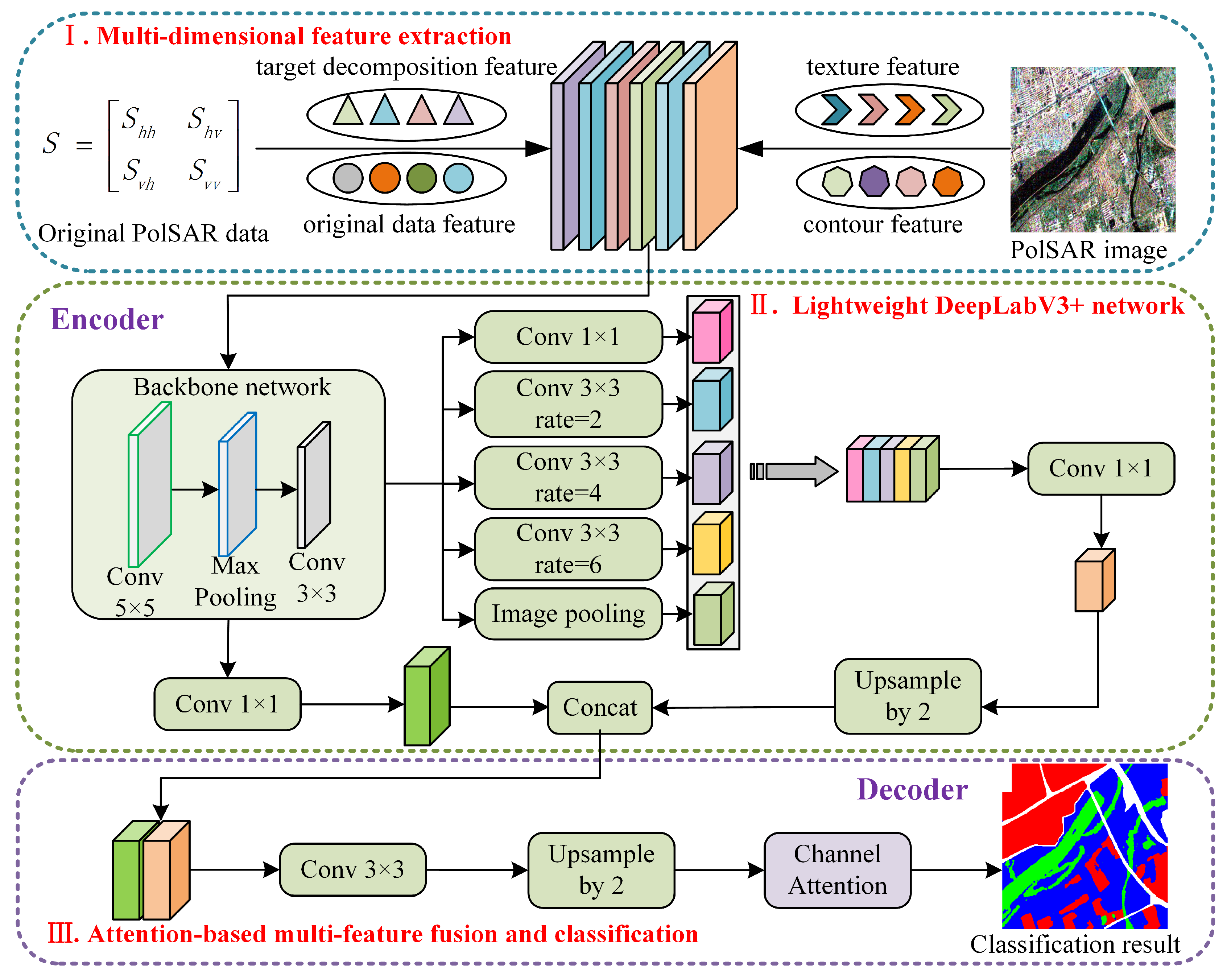
Figure 2.
Improved Xception network.
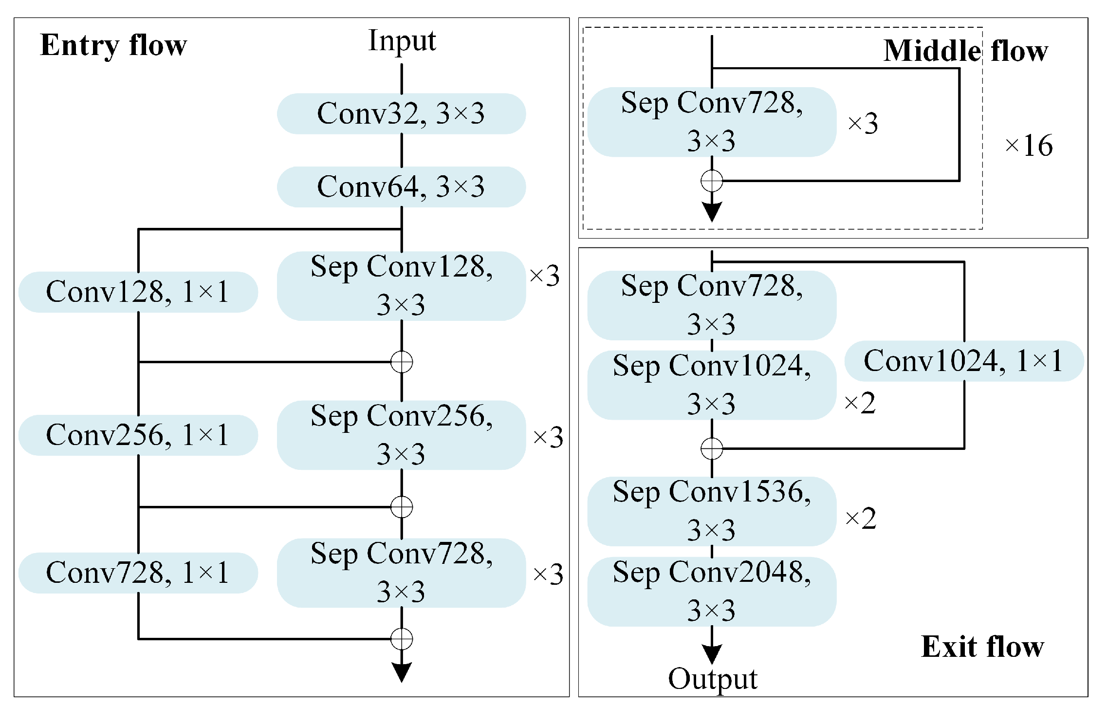
Figure 3.
Structure comparison between DeeplabV3+ and L-DeeplabV3+ networks, the yellow module represents the backbone network. (a) DeeplabV3+, (b) L-DeeplabV3+.
Figure 3.
Structure comparison between DeeplabV3+ and L-DeeplabV3+ networks, the yellow module represents the backbone network. (a) DeeplabV3+, (b) L-DeeplabV3+.
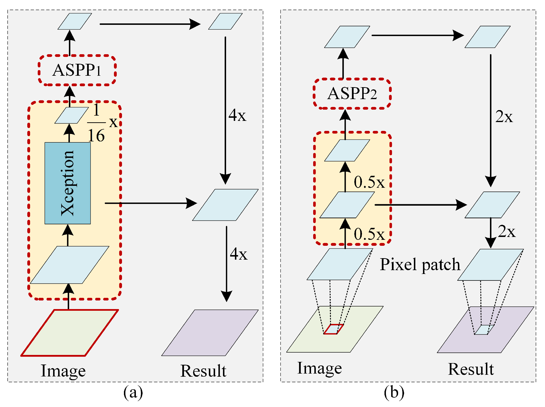
Figure 4.
The attention-based multi-feature fusion module.
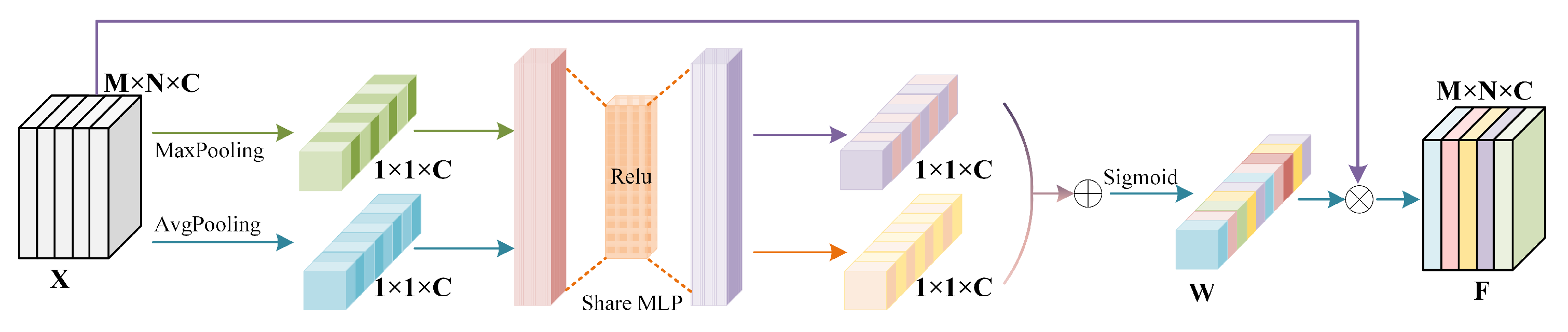
Figure 5.
PauliRGB images and the group-truth maps on the first three PolSAR data sets. (a) Xi’an data set; (b) Oberpfaffenhofen data set; (c) San Francisco data set;(d)Flevoland1 data set;(e)Flevoland1 data set.
Figure 5.
PauliRGB images and the group-truth maps on the first three PolSAR data sets. (a) Xi’an data set; (b) Oberpfaffenhofen data set; (c) San Francisco data set;(d)Flevoland1 data set;(e)Flevoland1 data set.
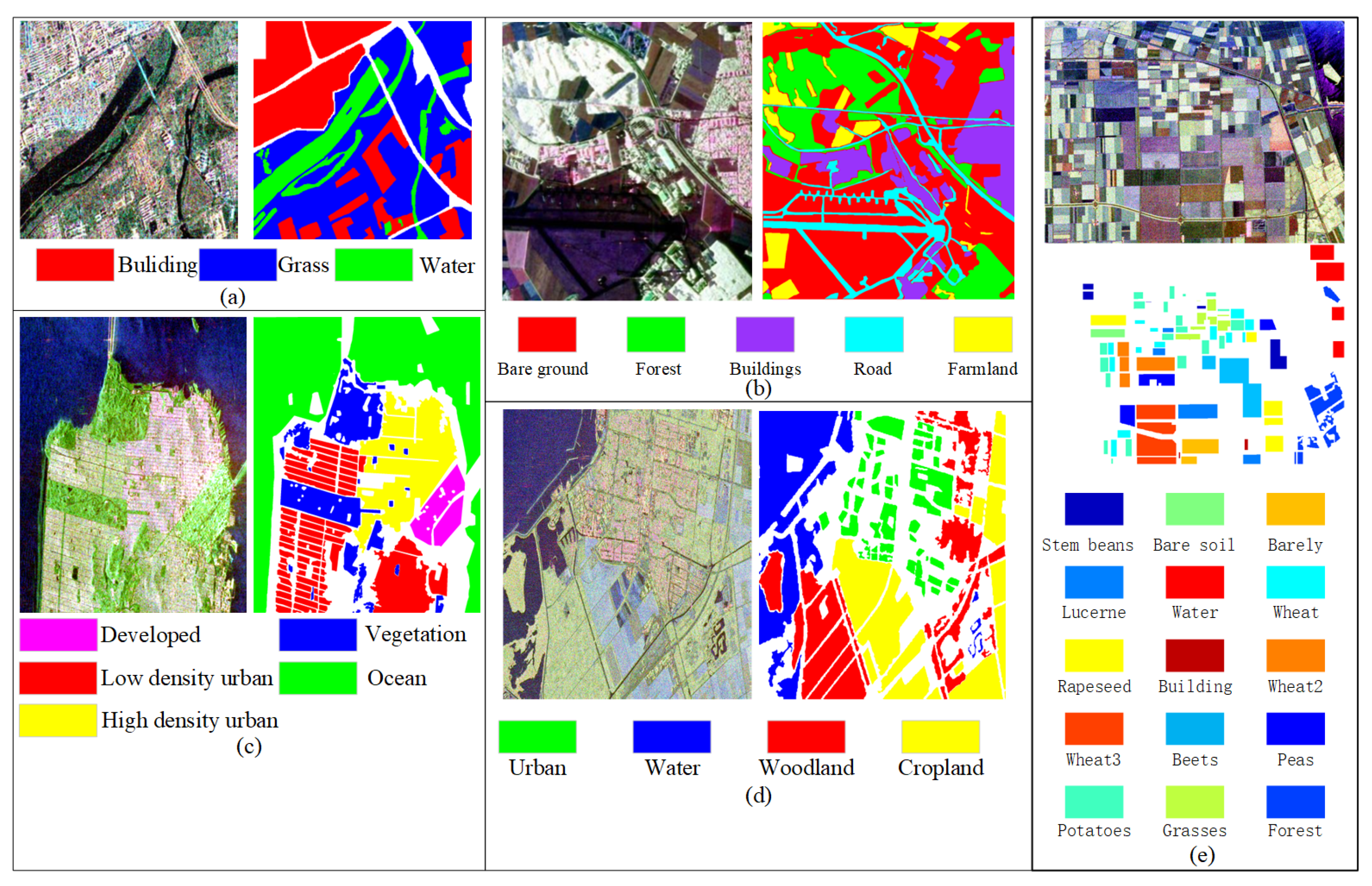
Figure 6.
Classification results of different methods on the Xi’an data set. (a)The label map of Xi’an data set; (b)The classification map by the Super-RF method; (c)The classification map by the CNN method; (d)The classification map by the CV-CNN method; (e)The classification map by the 3D-CNN method; (f)The classification map by the PolMPCNN method; (g)The classification map by the CEGCN method; (h)The classification map by the SGCN-CNN method; (i)The classification map by the proposed MLDnet method.
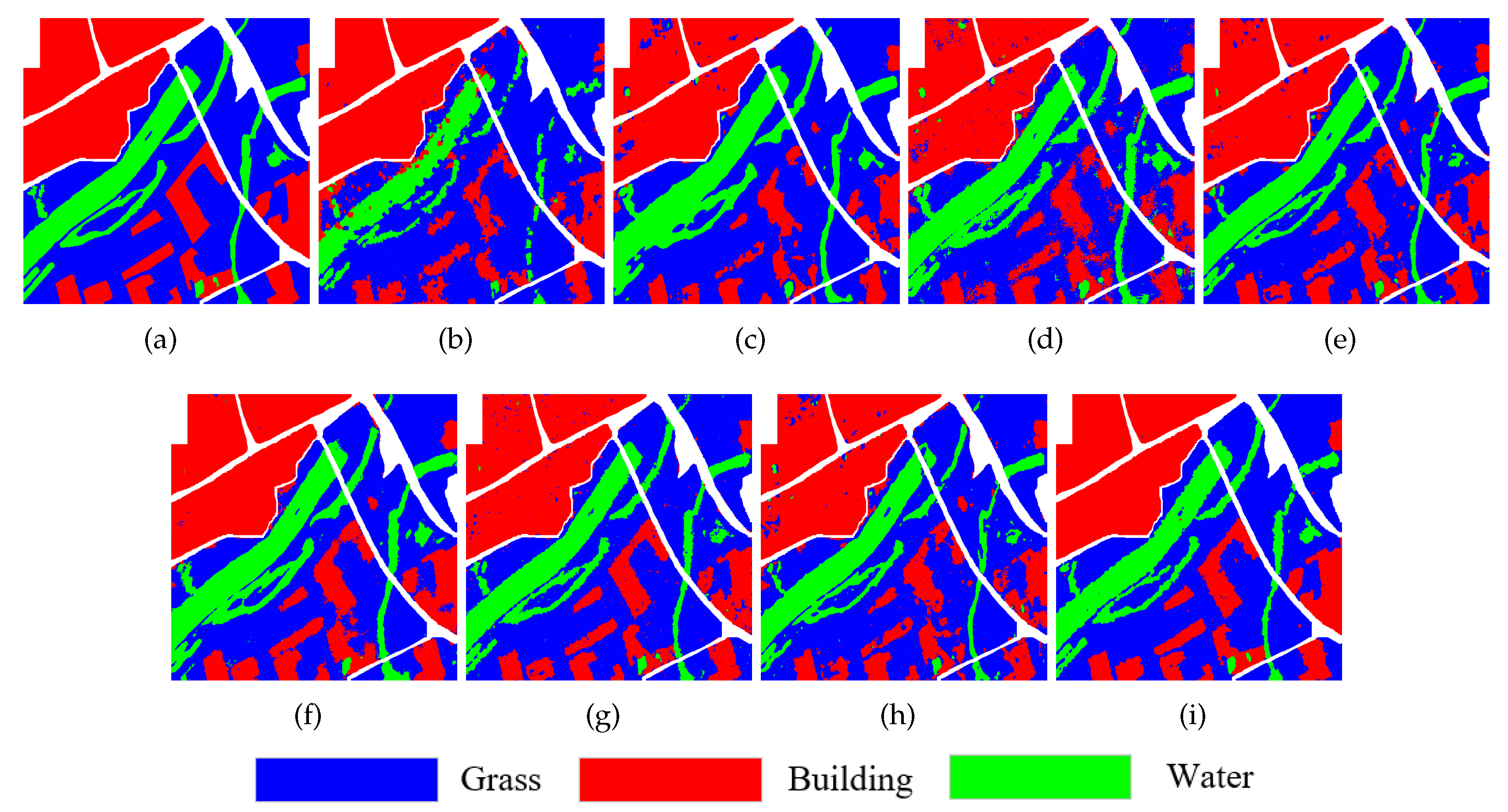
Figure 7.
Confusion matrix of Xi’an data set
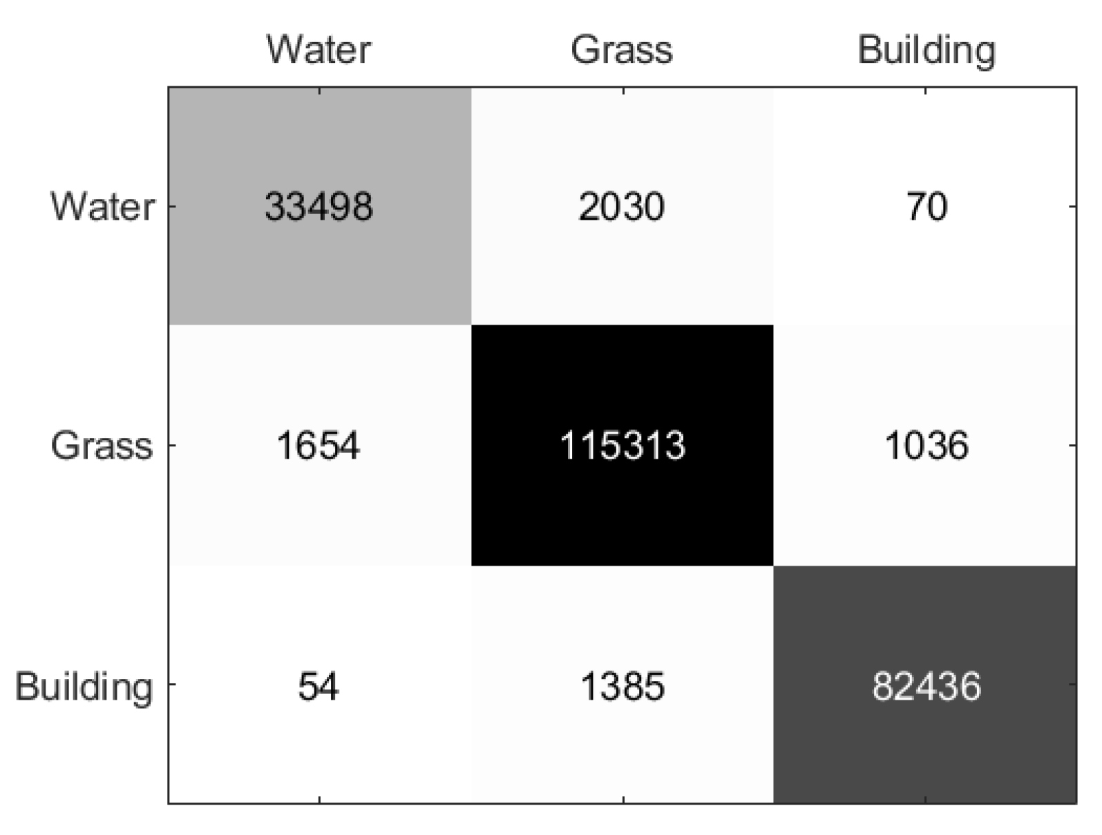
Figure 8.
Classification results of different methods on the Oberpfaffenhofen data set. (a)The label map of Oberpfaffenhofen data set; (b)The classification map by the Super-RF method; (c)The classification map by the CNN method; (d)The classification map by the CV-CNN method; (e)The classification map by the 3D-CNN method; (f)The classification map by the PolMPCNN method; (g)The classification map by the CEGCN method;(h)The classification map by the SGCN-CNN method; (i)The classification map by the proposed MLDnet method.
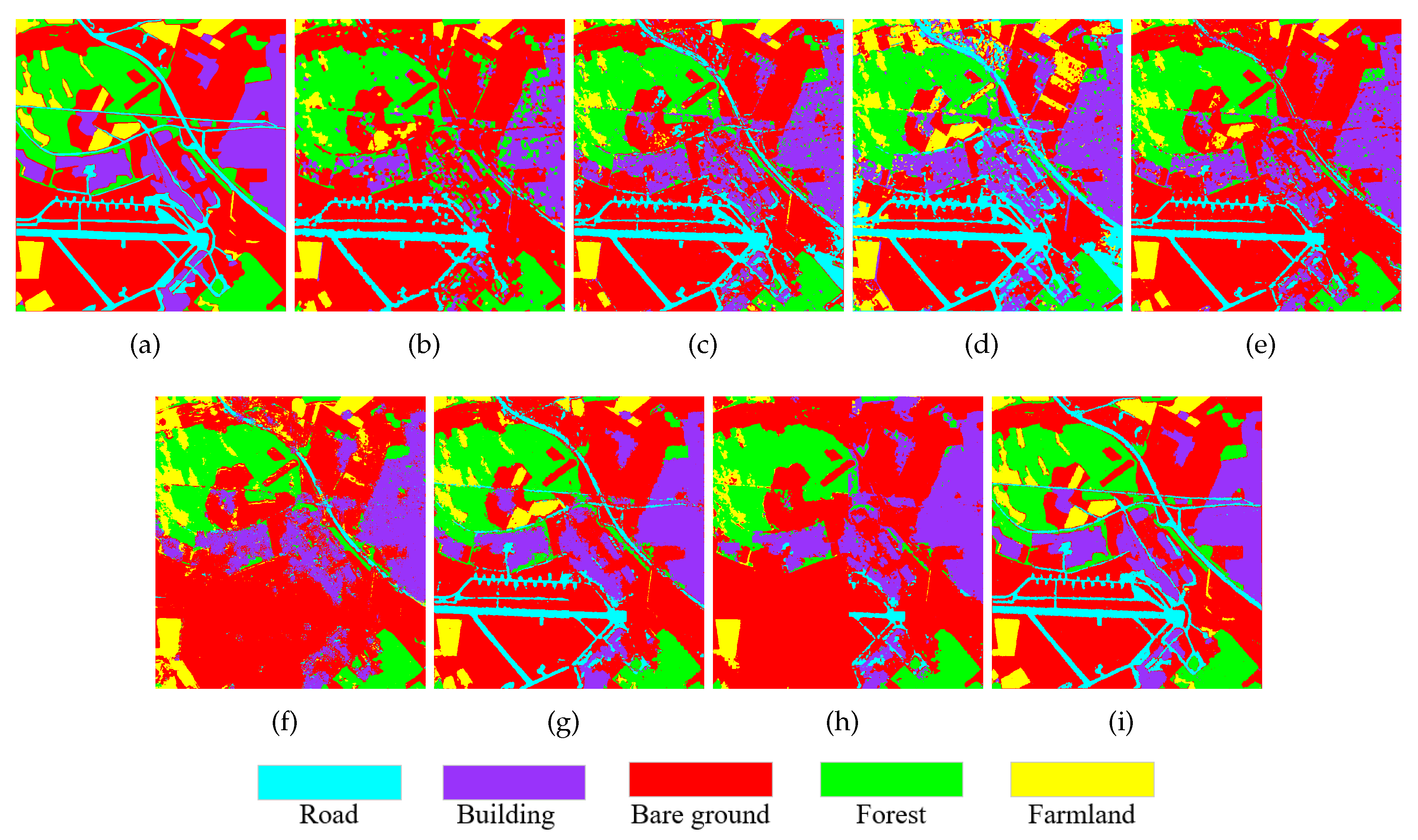
Figure 9.
Confusion matrix of Oberpfaffenhofen data set.
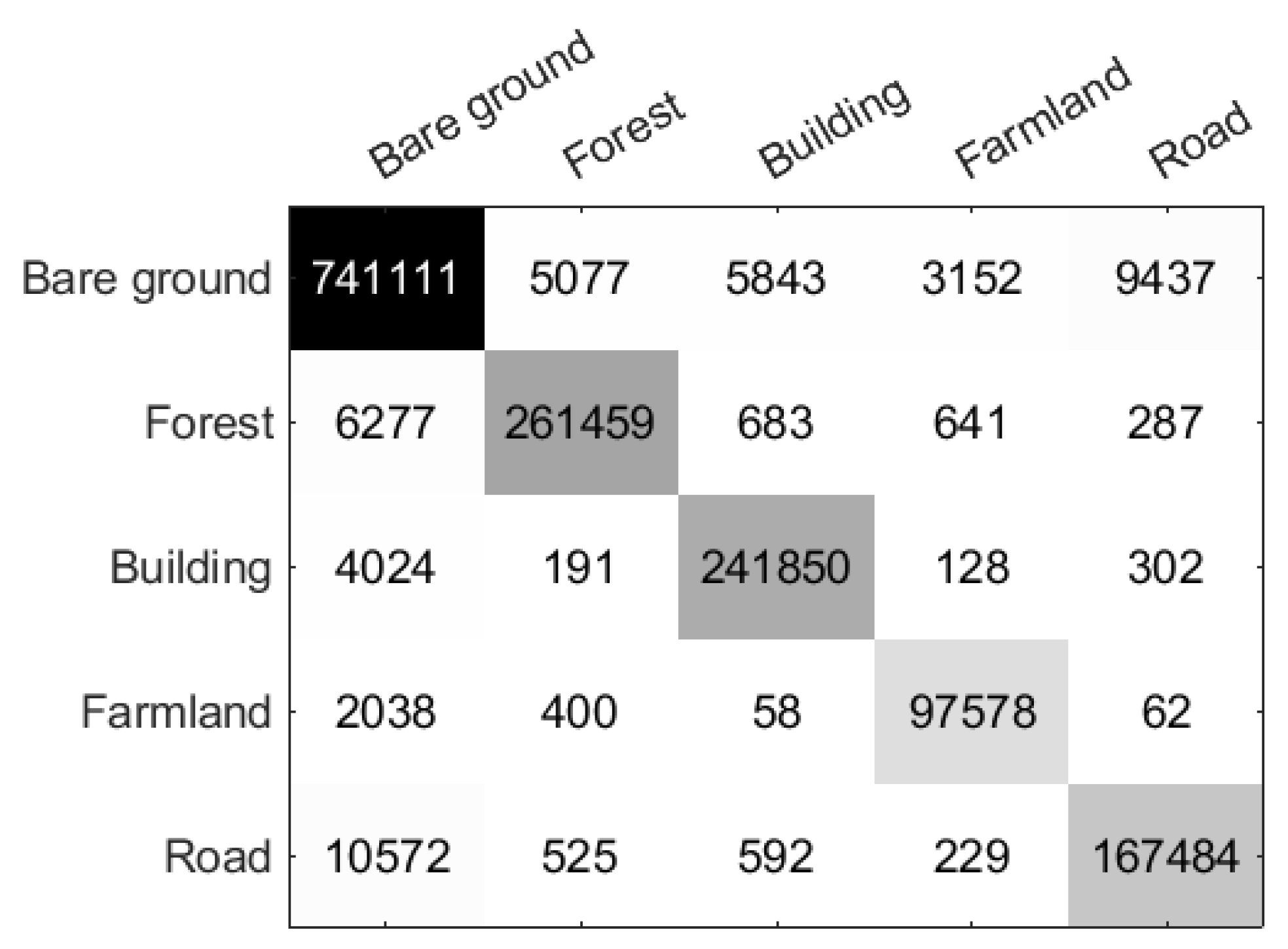
Figure 10.
Classification results of different methods on the San Francisco data set. (a)The label map of San Francisco data set; (b)The classification map by the Super-RF method; (c)The classification map by the CNN method; (d)The classification map by the CV-CNN method; (e)The classification map by the 3D-CNN method; (f)The classification map by the PolMPCNN method; (g)The classification map by the CEGCN method; (h)The classification map by the SGCN-CNN method; (i)The classification map by the proposed MLDnet method.
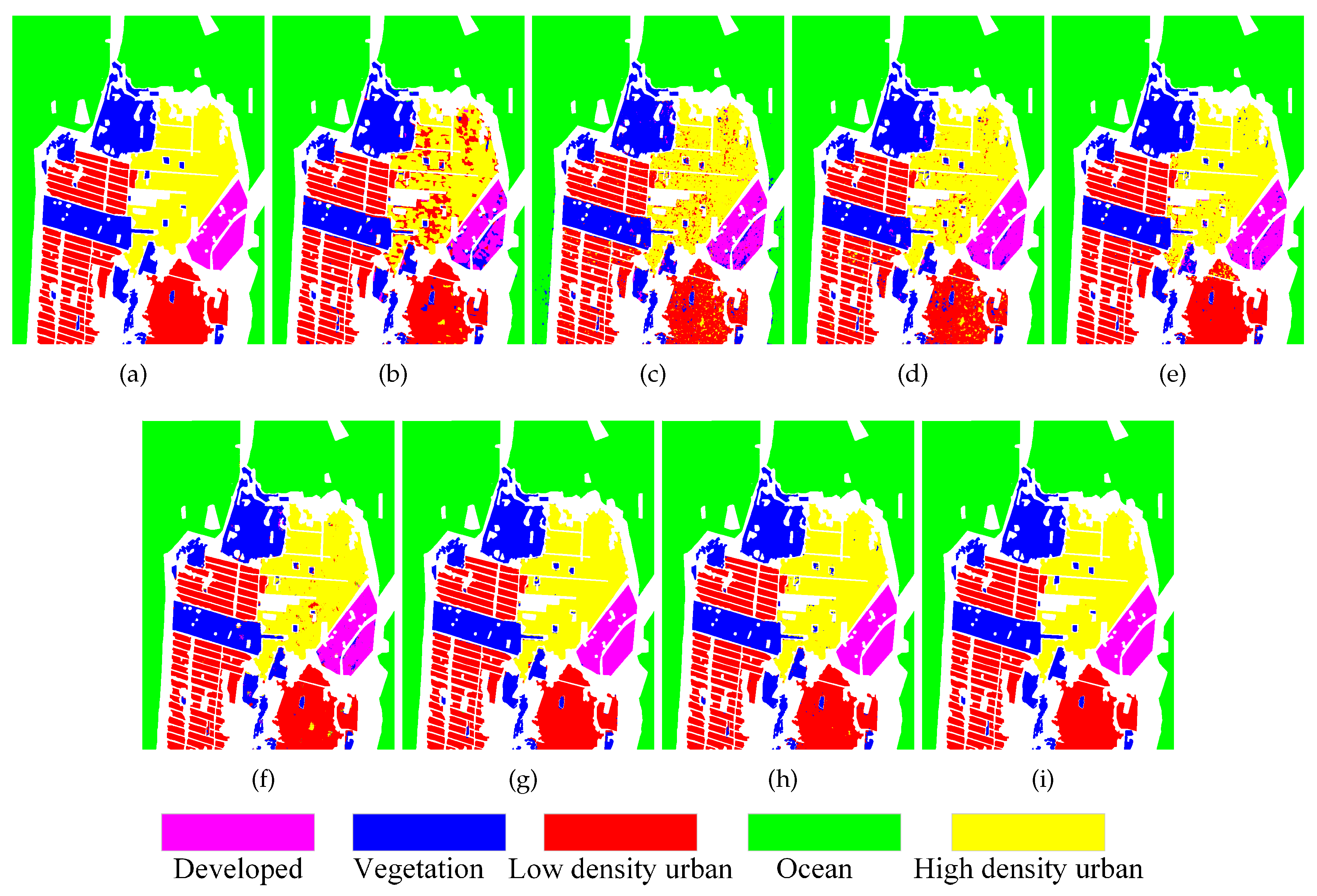
Figure 11.
Confusion matrix of San Francisco data set
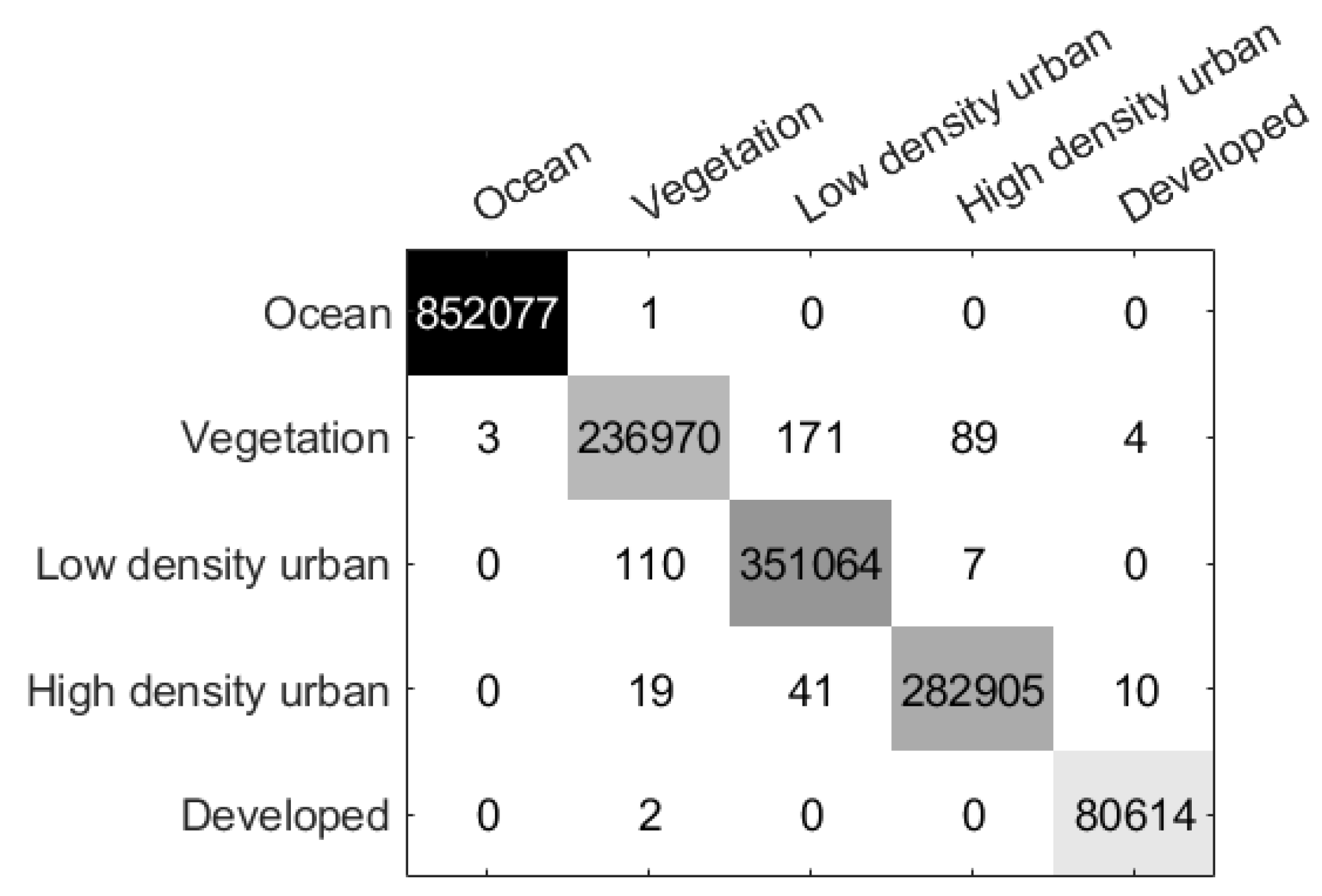
Figure 13.
Confusion matrix of Flevoland1 data set
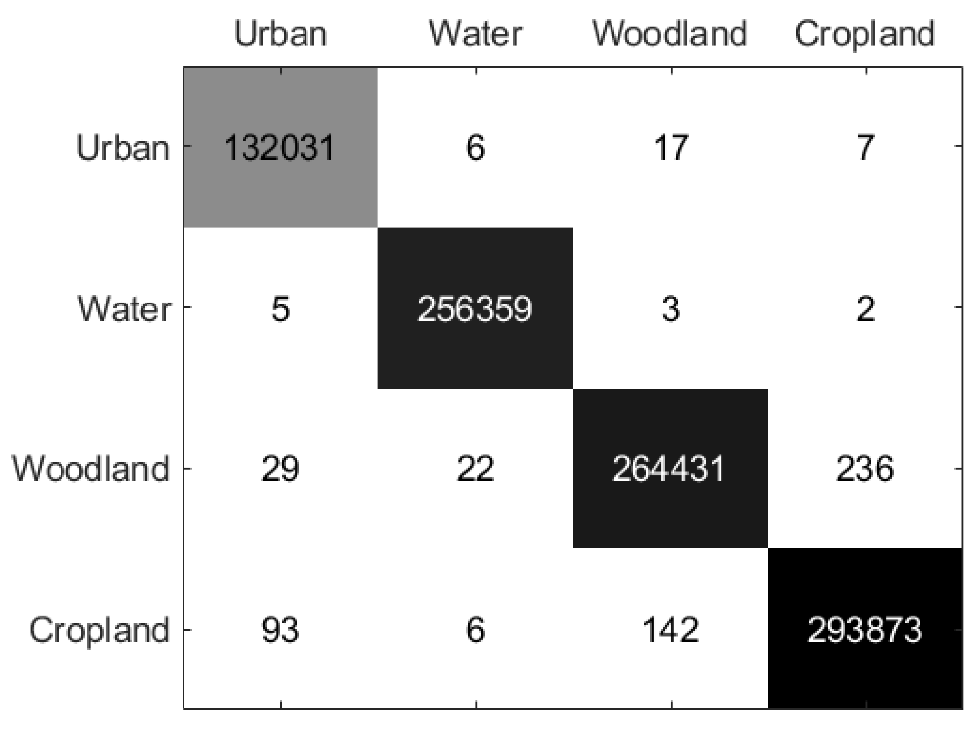
Figure 15.
Confusion matrix of Flevoland2 data set.
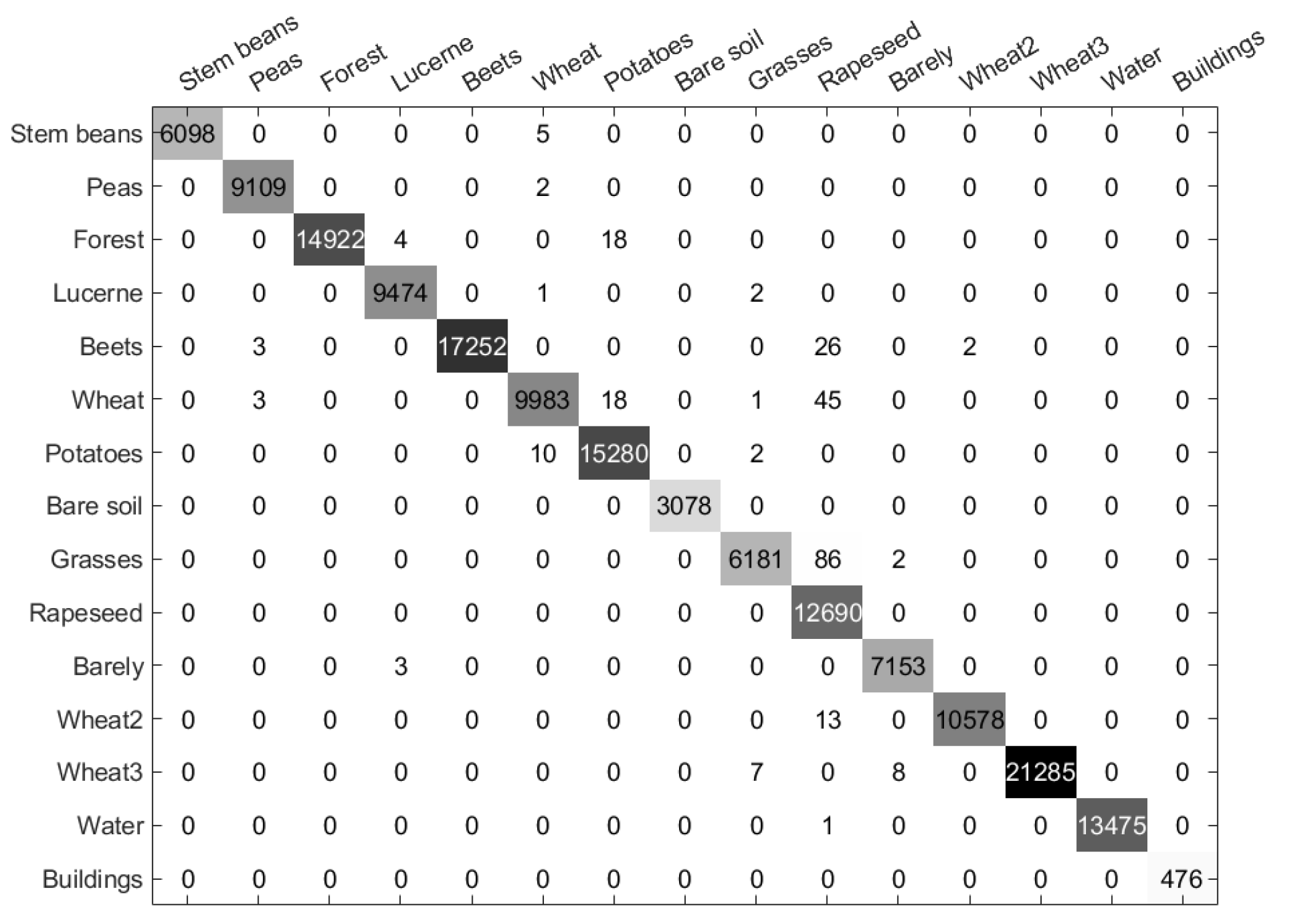
Figure 17.
Overall classification accuracy of five data sets under different sampling window sizes.
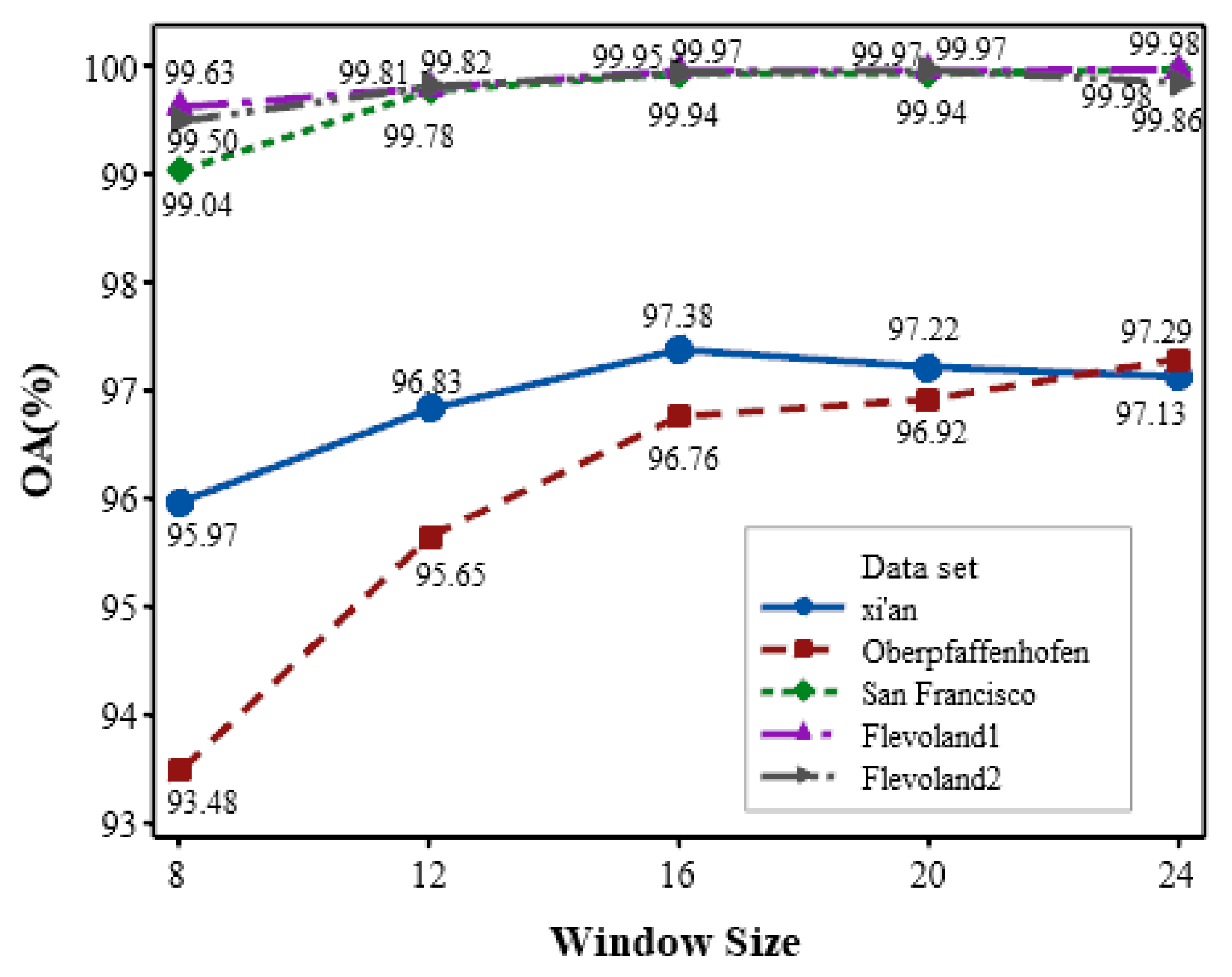
Figure 18.
Overall classification accuracy of training samples of five data sets at different sampling ratios.
Figure 18.
Overall classification accuracy of training samples of five data sets at different sampling ratios.
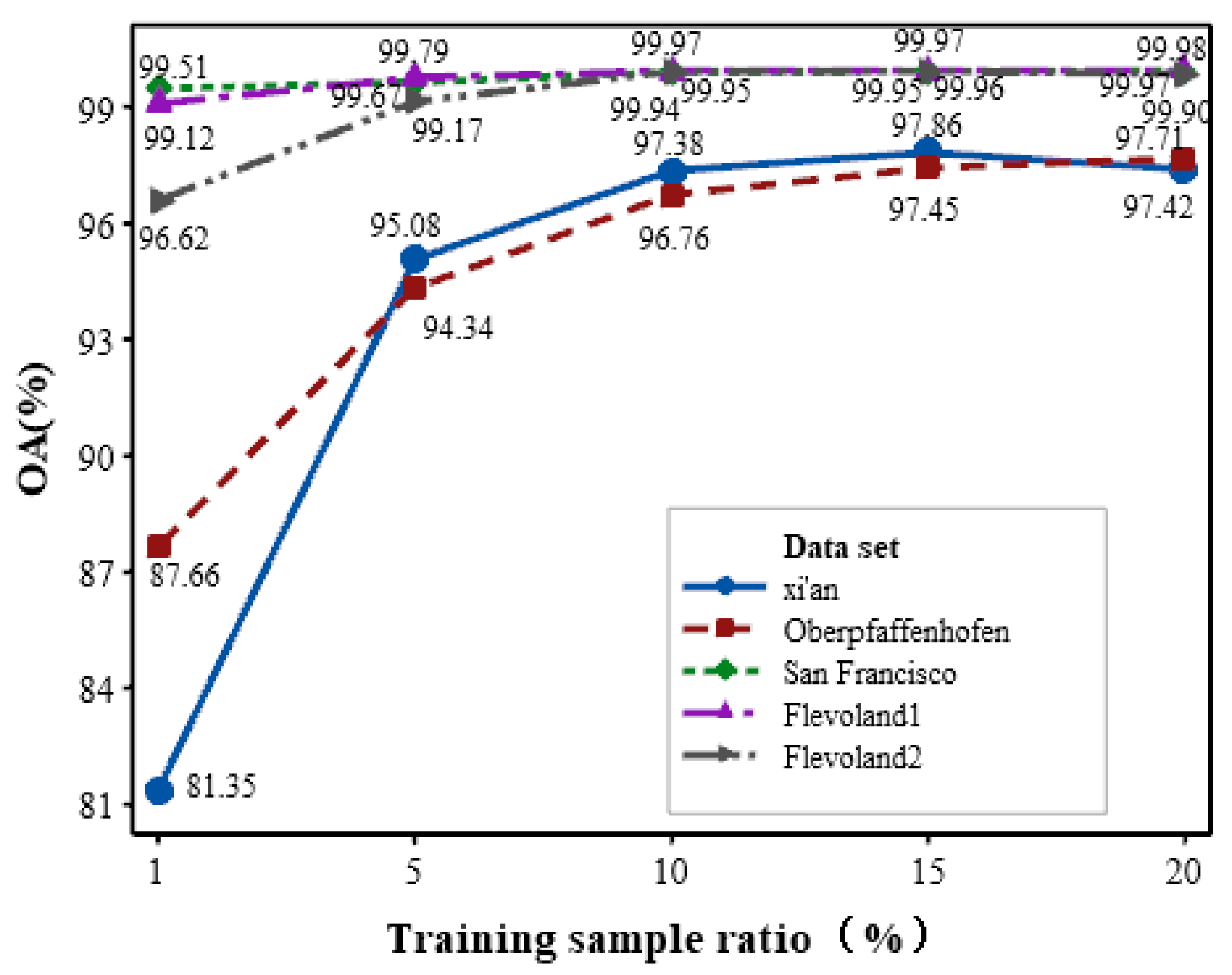

Table 1.
57-dimension features list
| Feature | Feature name | Feature parameter | number |
|---|---|---|---|
| Original data features | Scattering matrix elements |
, | 6 |
| Coherency matrix elements |
, | 9 | |
| SPAN | 1 | ||
| Target decomposition features |
Cloud and Pottier decomposition |
H,A, | 3 |
| Freeman decomposition | the surface, double-bounce and volume scattering power | 3 | |
| Huynen decomposition | ,, | 9 | |
| Co-polarization ratio | 1 | ||
| Cross-polarization ratio | 1 | ||
| Textural and contour features |
GLCM features | 4 | |
| 4 | |||
| 4 | |||
| / | 4 | ||
| Edge-line energy features |
/ | 4 | |
| 4 | |||
| Total | 57 |
Table 2.
Parameter comparison between DeeplabV3+ and L-DeeplabV3+ networks
| Network | DeeplabV3+ | L-DeeplabV3+ |
|---|---|---|
| Input feature map | ||
| Backbone network | Xception network | Conv+Maxpooling+Conv |
| ASPP | Conv,r=6,12,18 | Conv,r=2,4,6 |
Table 3.
Classification accuracy of different methods on Xi’an Data Set. (%)
| Class | Super-RF[17] | CNN[21] | CV-CNN[23] | 3D-CNN[60] | PolMPCNN[61] | CEGCN[62] | SGCN-CNN[63] | MLDnet |
|---|---|---|---|---|---|---|---|---|
| Water | 70.91 | 93.12 | 97.26 | 90.27 | 95.52 | 94.47 | 86.57 | 94.10 |
| Grass | 94.97 | 92.82 | 85.97 | 93.60 | 90.95 | 96.50 | 93.33 | 97.72 |
| Building | 90.94 | 85.31 | 91.43 | 93.91 | 97.68 | 96.54 | 90.12 | 98.28 |
| OA | 89.94 | 90.21 | 89.59 | 93.21 | 94.01 | 96.21 | 91.18 | 97.38 |
| AA | 85.61 | 90.42 | 91.55 | 92.60 | 94.71 | 95.83 | 90.01 | 96.70 |
| Kappa | 83.02 | 83.83 | 83.18 | 88.77 | 90.25 | 93.74 | 85.33 | 95.67 |
Table 4.
Classification accuracy of different methods on Oberpfaffenhofen Data Set. (%)
| Class | Super-RF[17] | CNN[21] | CV-CNN[23] | 3D-CNN[60] | PolMPCNN[61] | CEGCN[62] | SGCN-CNN[63] | MLDnet |
|---|---|---|---|---|---|---|---|---|
| Bare ground | 91.76 | 85.95 | 68.86 | 91.76 | 86.92 | 93.14 | 92.94 | 96.97 |
| Forest | 85.26 | 83.22 | 81.16 | 84.59 | 82.51 | 90.13 | 81.96 | 96.17 |
| Building | 59.55 | 83.50 | 87.52 | 83.91 | 85.82 | 94.46 | 87.60 | 95.77 |
| Farmland | 57.28 | 53.44 | 70.49 | 65.33 | 65.65 | 80.70 | 32.02 | 95.50 |
| Road | 49.19 | 67.41 | 76.20 | 50.34 | 10.38 | 66.14 | 14.67 | 93.78 |
| OA | 78.40 | 80.87 | 74.88 | 82.82 | 75.82 | 88.93 | 77.29 | 96.19 |
| AA | 68.59 | 74.70 | 76.85 | 75.19 | 66.26 | 84.91 | 61.84 | 95.64 |
| Kappa | 67.42 | 72.03 | 65.73 | 74.28 | 63.46 | 83.66 | 64.76 | 94.44 |
Table 5.
Classification accuracy of different methods on San Francisco Data Set. (%)
| Class | Super-RF[17] | CNN[21] | CV-CNN[23] | 3D-CNN[60] | PolMPCNN[61] | CEGCN[62] | SGCN-CNN[63] | MLDnet |
|---|---|---|---|---|---|---|---|---|
| Ocean | 99.98 | 99.59 | 99.99 | 100 | 99.58 | 99.99 | 100 | 100 |
| Vegetation | 93.89 | 93.51 | 96.42 | 94.80 | 95.63 | 97.87 | 97.40 | 99.89 |
| Low density urban | 97.31 | 94.47 | 94.51 | 97.96 | 99.39 | 99.58 | 99.48 | 99.97 |
| High density urban | 77.76 | 92.57 | 96.37 | 97.61 | 98.57 | 99.49 | 99.48 | 99.98 |
| Developed | 81.00 | 90.31 | 95.92 | 96.25 | 96.81 | 99.88 | 99.95 | 100 |
| OA | 94.33 | 96.28 | 97.71 | 98.38 | 98.93 | 99.55 | 99.47 | 99.97 |
| AA | 89.99 | 94.09 | 96.64 | 97.32 | 98.08 | 99.36 | 99.26 | 99.97 |
| Kappa | 91.81 | 94.65 | 96.70 | 97.66 | 98.46 | 99.35 | 99.24 | 99.96 |
Table 6.
Classification accuracy of different methods on Flevoland1 Data Set. (%)
| Class | Super-RF[17] | CNN[21] | CV-CNN[23] | 3D-CNN[60] | PolMPCNN[61] | CEGCN[62] | SGCN-CNN[63] | MLDnet |
|---|---|---|---|---|---|---|---|---|
| Urban | 81.84 | 88.87 | 96.26 | 94.74 | 96.29 | 99.45 | 99.73 | 99.98 |
| Water | 98.69 | 99.68 | 99.85 | 98.87 | 99.14 | 99.65 | 99.77 | 99.99 |
| Woodland | 94.92 | 95.59 | 96.48 | 96.03 | 98.77 | 98.96 | 99.58 | 99.89 |
| Cropland | 94.16 | 93.16 | 93.94 | 96.75 | 98.66 | 99.47 | 99.63 | 99.92 |
| OA | 93.88 | 95.01 | 96.57 | 96.84 | 98.49 | 99.37 | 99.67 | 99.94 |
| AA | 92.40 | 94.33 | 96.63 | 96.60 | 98.21 | 99.38 | 99.68 | 99.95 |
| Kappa | 91.61 | 93.18 | 95.33 | 95.69 | 97.94 | 99.14 | 99.55 | 99.92 |
Table 7.
Classification accuracy of different methods on Flevoland2 Data Set. (%)
| Class | Super-RF[17] | CNN[21] | CV-CNN[23] | 3D-CNN[60] | PolMPCNN[61] | CEGCN[62] | SGCN-CNN[63] | MLDnet |
|---|---|---|---|---|---|---|---|---|
| Stem beans | 96.77 | 99.58 | 99.72 | 88.45 | 99.79 | 98.54 | 95.41 | 99.96 |
| Peas | 98.64 | 97.95 | 99.99 | 85.90 | 99.00 | 85.70 | 99.63 | 100 |
| Forest | 95.88 | 97.36 | 99.82 | 99.85 | 99.97 | 99.95 | 99.89 | 99.98 |
| Lucerne | 96.63 | 88.95 | 98.17 | 96.26 | 98.45 | 100 | 99.84 | 99.98 |
| Beets | 99.05 | 93.86 | 98.66 | 99.21 | 95.52 | 99.49 | 98.91 | 99.97 |
| Wheat | 95.70 | 97.43 | 99.22 | 98.57 | 98.00 | 98.54 | 97.60 | 99.69 |
| Potatoes | 96.04 | 94.98 | 99.14 | 98.14 | 98.76 | 99.40 | 99.56 | 99.96 |
| Bare soil | 94.57 | 99.09 | 100 | 99.71 | 99.84 | 100 | 100 | 99.89 |
| Grasses | 84.03 | 76.51 | 99.94 | 76.50 | 95.71 | 88.32 | 90.96 | 99.68 |
| Rapeseed | 53.13 | 83.90 | 94.18 | 94.83 | 93.55 | 99.30 | 97.79 | 99.98 |
| Barley | 100 | 81.75 | 99.58 | 75.36 | 40.25 | 100 | 91.74 | 100 |
| Wheat2 | 79.93 | 95.26 | 99.41 | 97.04 | 95.97 | 99.95 | 99.85 | 100 |
| Wheat3 | 99.39 | 98.47 | 99.37 | 99.77 | 93.88 | 99.97 | 99.78 | 99.97 |
| Water | 100 | 99.81 | 99.99 | 100 | 91.27 | 100 | 99.96 | 100 |
| Buildings | 0 | 86.01 | 100 | 50.63 | 96.01 | 80.88 | 96.22 | 100 |
| OA | 92.18 | 93.96 | 98.96 | 95.28 | 93.82 | 98.32 | 98.50 | 99.95 |
| AA | 85.98 | 92.73 | 99.15 | 90.68 | 93.06 | 96.67 | 97.81 | 99.94 |
| Kappa | 91.44 | 93.40 | 98.87 | 94.84 | 93.27 | 98.16 | 98.36 | 99.95 |
Table 8.
Classification accuracy of different submodule networks on five experimental data sets (%)
| Data set | Xi’an | Oberpfaffenhofen | Flevoland1 | Flevoland2 | San Francisco | |||||
|---|---|---|---|---|---|---|---|---|---|---|
| Accuracy | OA | Kappa | OA | Kappa | OA | Kappa | OA | Kappa | OA | Kappa |
| wihtout MF | 96.86 | 94.83 | 93.82 | 91.04 | 99.19 | 98.89 | 98.92 | 98.82 | 99.80 | 99.72 |
| without L-deeplabV3+ | 96.73 | 94.62 | 95.50 | 93.47 | 99.83 | 99.78 | 99.77 | 99.75 | 99.96 | 99.95 |
| without Attention | 96.29 | 93.93 | 96.52 | 94.93 | 99.86 | 99.81 | 99.55 | 99.50 | 99.75 | 99.64 |
| MLDnet | 97.38 | 95.67 | 96.76 | 95.29 | 99.94 | 99.92 | 99.95 | 99.95 | 99.97 | 99.96 |
Table 9.
Classification accuracy of Deeplabv3+ and L-deeplabV3+ networks on Flevoland2 data set. (%)
Table 9.
Classification accuracy of Deeplabv3+ and L-deeplabV3+ networks on Flevoland2 data set. (%)
| Class | DeeplabV3+[64] | L-deeplabV3+ |
|---|---|---|
| Stem beans | 95.61 | 99.96 |
| Peas | 70.36 | 100 |
| Forest | 89.49 | 99.97 |
| Lucerne | 97.51 | 99.87 |
| Beets | 94.72 | 100 |
| Wheat | 84.74 | 99.25 |
| Potatoes | 92.93 | 99.40 |
| Bare soil | 97.23 | 100 |
| Grasses | 96.04 | 99.96 |
| Rapeseed | 95.84 | 99.38 |
| Barley | 96.71 | 100 |
| Wheat2 | 92.58 | 96.52 |
| Wheat3 | 84.41 | 99.84 |
| Water | 90.43 | 100 |
| Buildings | 98.40 | 90.90 |
| OA | 97.59 | 99.55 |
| Kappa | 92.87 | 99.50 |
Table 10.
Classification accuracy of different types of feature input on Xi’an data set. (%)
| Class | feature 1 | feature 2 | feature 3 | multi-features |
|---|---|---|---|---|
| Water | 91.25 | 93.79 | 89.24 | 94.10 |
| Grass | 95.31 | 89.57 | 97.15 | 97.72 |
| Building | 95.31 | 89.57 | 97.15 | 98.28 |
| OA | 91.39 | 93.25 | 95.98 | 97.38 |
| AA | 90.83 | 93.85 | 94.53 | 96.70 |
| Kappa | 85.69 | 89.00 | 93.33 | 95.67 |
Table 11.
Classification accuracy of different positions and numbers of channel attention modules on Xi’an data set. (%)
Table 11.
Classification accuracy of different positions and numbers of channel attention modules on Xi’an data set. (%)
| Class | front1 | front2 | front3 | behind1 | behind2 | behind3 |
|---|---|---|---|---|---|---|
| Water | 86.95 | 77.91 | 79.65 | 94.10 | 80.48 | 79.99 |
| Grass | 92.27 | 96.00 | 94.06 | 97.72 | 97.57 | 92.03 |
| Building | 94.90 | 92.34 | 93.90 | 98.28 | 88.78 | 94.43 |
| OA | 92.40 | 91.99 | 91.85 | 97.38 | 91.91 | 91.07 |
| AA | 91.37 | 88.75 | 89.20 | 96.70 | 88.94 | 88.82 |
| Kappa | 87.50 | 86.58 | 86.40 | 95.67 | 86.38 | 85.20 |
Table 12.
Running time of different methods on Xi’an data set.(s)
| Super-RF | CNN | CV-CNN | 3D-CNN | PolMPCNN | CEGCN | SGCN-CNN | DeeplabV3+ | MLDnet | |
|---|---|---|---|---|---|---|---|---|---|
| Training time | 59.22 | 150.59 | 3463.20 | 121.84 | 21600.35 | 129.43 | 30.59 | 1543.21 | 511.10 |
| Test time | 1.85 | 10.56 | 38.43 | 22.80 | 327.53 | 4.45 | 3.00 | 53.50 | 23.48 |
Disclaimer/Publisher’s Note: The statements, opinions and data contained in all publications are solely those of the individual author(s) and contributor(s) and not of MDPI and/or the editor(s). MDPI and/or the editor(s) disclaim responsibility for any injury to people or property resulting from any ideas, methods, instructions or products referred to in the content. |
© 2025 by the authors. Licensee MDPI, Basel, Switzerland. This article is an open access article distributed under the terms and conditions of the Creative Commons Attribution (CC BY) license (http://creativecommons.org/licenses/by/4.0/).
Copyright: This open access article is published under a Creative Commons CC BY 4.0 license, which permit the free download, distribution, and reuse, provided that the author and preprint are cited in any reuse.


