
Submitted:
08 April 2024
Posted:
09 April 2024
You are already at the latest version
Abstract
Polarimetric features extracted from polarimetric synthetic aperture radar (PolSAR) images contain abundant scattering information of objects. Utilizing this information for PolSAR image classification can improve accuracy and enhance object monitoring. Although significant progress has been achieved in related research, there are still issues such as insufficient utilization of polarimetric information and features. In this paper, a deep learning classification method based on polarimetric channel power features for PolSAR is proposed. The distinctive characteristic of this method is that the polarimetric features inputted into the deep learning network are the power values of polarimetric channels, where these channels are treated equivalently and contain complete polarimetric information. In terms of experimental comparative study, besides polarimetric power combinations, three different data input schemes were employed as data for the input end of the convolutional neural network (CNN), taking into account existing research. The neural networks utilizes the extracted polarimetric features to classify images, and the classification accuracy analysis is employed to compare the strengths and weaknesses of different input schemes. It is worth mentioning that the polarized characteristics of the data input scheme mentioned in this article have been derived through rigorous mathematical deduction, and each polarimetric feature has clear physical meaning. By testing different data input schemes on the Gaofen-3 (GF-3) PolSAR image, the experimental results show that the method proposed in this article outperforms existing methods and can improve the accuracy of classification to a certain extent, validating the effectiveness of this method in large-scale area classification.
Keywords:
Polarimetric Synthetic Aperture Radar (PolSAR)
; Reflection Symmetric Decomposition (RSD)
; Data Input Scheme
; Land Classification
; Polarimetric Scattering Characteristics.
1. Introduction
Polarimetric synthetic aperture radar (PolSAR) is able to acquire comprehensive polarization information of land targets, and it can actively detect targets in all-weather and all-day conditions. Compared to single and dual polarized images, PolSAR images contain a significant amount of back-scattering information of the objects [1]. Currently, PolSAR classification methods mainly include polarization feature-based approaches, statistical distribution characteristics of PolSAR data, and deep learning classification methods [2,3,4,5,6,7].
A large number of scholars have conducted in-depth research on PolSAR classification and achieved good results. The method mainly adopts polarization decomposition to extract the polarization scattering information of the targets and further classify them based on these features. Cloude et al. have done a lot of work in PolSAR classification [8,9]. C. Lardeux et al. [10] used support vector machine (SVM) classifier to extract polarization features from PolSAR images of different frequencies and perform classification using these features. Dickinson et al. [11] classified targets in multiple scenarios using polarization decomposition.
The classification method based on statistical features of PolSAR images mainly utilizes the difference in statistical characteristics of target objects to classify different targets in the images. Lee et al. [12] used polarization decomposition and unsupervised classification, based on complex Wishart classifier, to classify PolSAR images. Silva et al. [13] used the minimum random distance and Wishart distribution to segment the targets in PolSAR images. Chen et al. [14] used the method of polarimetric similarity and maximum minimum scattering features to improve the accuracy of classification. Wu et al. [15] used a domain-based Wishart MRF method to classify PolSAR images and make good results compared with other methods.
Although the above methods have achieved good results, they are all based on pixel-level classification, ignoring the relationship between the classified pixels and their neighborhoods. Liu et al. [16] used the information from the center pixel as well as the surrounding neighborhood pixels, combined them into superpixels, and used them as the smallest classification unit to classify PolSAR images, resulting in better classification results.
Many researchers have studied the polarization decomposition method, and some famous algorithms include Pauli decomposition [17], SDH decomposition [18], Freeman decomposition [19], Yamaguchi decomposition [20], and reflection symmetrical decomposition(RSD) [21]. Freeman-Durden decomposition [22], Van Zyl decomposition [23], H/A/Alpha decomposition [24], Huynen decomposition [25], Cameron decomposition [26], and Krogager decomposition [27], are also commonly used. These polarization decomposition algorithms have been applied to PolSAR land cover classification by relevant researchers. Nie et al. [28] utilized 12 polarization features obtained from Freeman-Durden decomposition, Van Zyl decomposition and H/A/Alpha decomposition and achieved good classification results on limited samples using an enhanced learning framework. Wang et al. [29] applied the Freeman-Durden decomposition method and used a feature fusion strategy to classify PolSAR images of the Flevoland region. Ren et al. [30] utilized polarization scattering features obtained from T-matrix, Pauli decomposition, H/A/Alpha decomposition, and Freeman decomposition.Zhang et al.[57] applied the RSD method to extract polarimetric features from Gaofen3 images and obtain good results.
Deep learning methods extract information of land targets through a certain number of network layers and utilize deep-level features extracted from the targets to classify objects in the image. Compared to traditional classification methods or machine learning, deep learning can more fully exploit the scattering characteristics inherent in land targets. In PolSAR data analysis, deep belief networks [31], stacked autoencoders [32], generative adversarial networks [33], convolutional neural networks [34,35], and deep stacked networks have achieved tremendous success [36,37,38]. Deep learning is a hierarchical learning method, and features extracted through this method are more discriminative [39]. Therefore, it demonstrates excellent performance in PolSAR image classification and target detection [40,41,42,43,44,45,46,47,48].
The PolSAR image contains multiple polarimetric characteristics and raw information of objects. Adopting an appropriate polarimetric decomposition method could extract features that represent objects, which benefits subsequent neural networks in classifying those features. Through existing research, it has been found that the most commonly used data input scheme is the 6-parameter data input scheme [49,50,51]. This method uses the total power of polarization, the two main diagonal elements of the polarimetric coherence matrix (T-matrix), and the correlation coefficient between non-main diagonal elements of the matrix. Although this data input scheme has achieved good classification of objects using improved neural networks, some parameters do not have clear physical meanings at the polarimetric feature level, and from the perspective of polarimetric information content, it is not complete. This prompts us to seek a data input scheme that can have physical interpretability and a more complete utilization of polarimetric information at the polarimetric feature level.
This article presents a PolSAR deep learning classification method based on the power values of polarimetric channels. It mainly utilizes horizontal, vertical, left-handed, and right-handed polarization, as well as other equivalent power values of different polarimetric channels as input schemes for the neural network. This data input scheme is essentially a combination of polarimetric powers. The channels are equivalent to each other and represent power values under different polarization observations, and their addition and subtraction operations have clear physical meanings. Three polarimetric data input schemes were used, and then these polarimetric features were input into the neural network model to classify objects. The specific implementation process is shown in Figure 1. What is worth noting is that the proposed classification scheme deserves emphasis in the following aspects.
First, the surface scattering, volume scattering, secondary scattering power, and total power polarization are used as the basic data input scheme 1. Based on this, according to existing research, the polarimetric coherence matrix and the correlation coefficient between the non-diagonal elements of the matrix are utilized as data input scheme 2. Finally, based on mathematical derivation, the linear polarization and circular polarization-based horizontal, vertical, left-handed, right-handed polarization power characteristics, as well as the three main diagonal elements of the non-polarimetric coherence matrix and total power polarization, are adopted as input scheme 3. Each polarization characteristic in this data input scheme has clear physical significance.
The proposed data input scheme, compared to the other two contrast schemes, to some extent increases the amount of information input, and under the same neural network conditions, the final PolSAR image classification accuracy has been improved to a certain extent.
2. Method
Figure 1 depicts the data processing flow, which mainly includes data preprocessing, polarization decomposition, polarization feature normalization, data input scheme, and neural network classification.
2.1. Polarization Decomposition Method Based on Polarimetric Scattering Features
Target decomposition is a primary approach in polarimetric SAR data processing, which essentially represents pixels as weighted sums of several scattering mechanisms. In 1998, scholars Anthony Freeman and Stephen L. Durden proposed the first model-based, non-coherent polarimetric decomposition algorithm [22], hereinafter referred to as the Freeman decomposition. The initial purpose of the Freeman decomposition was to facilitate viewers of multi-view SAR images in intuitively distinguishing the major scattering mechanisms of objects.
The Freeman decomposition is entirely based on the back-scattering data observed by radar and its decomposed components have corresponding physical meanings. Therefore, it later became known as the first model-based, non-coherent polarimetric decomposition algorithm. The introduction of the Freeman decomposition was pioneering at that time. After the proposal of the Freeman decomposition, as scholars extensively utilized and further researched it, they found three main issues with the decomposition method: overestimation of volume scattering components, presence of negative power components in the results, and loss of polarization information. Through research, it was discovered that these three problems are not completely independent. For example, the overestimation of volume scattering components is one of the reasons for the existence of negative power values in subsequent surface scattering and double bounce components, and the loss of polarization information is also one of the reasons for the inappropriate estimation of power values of the volume scattering component.
In 2005, Yamaguchi et al. proposed the second model-based, non-coherent polarimetric decomposition algorithm [20]. This algorithm includes four scattering components, hereinafter referred to as the Yamaguchi algorithm. The Yamaguchi decomposition introduced helical scattering as the fourth scattering component, breaking the reflection symmetry assumption of the Freeman decomposition. This expansion made the algorithm applicable to a wider range of scenarios and achieved better experimental results in urban area analysis. The improved volume scattering model proposed by Yamaguchi opened up the research direction of enhancing the performance of model-based, non-coherent polarimetric decomposition algorithms through improving the scattering model. Both of the above points were pioneering work. However, the Yamaguchi algorithm did not provide a theoretical basis for selecting helical scattering as the fourth component, and according to their paper, the selection of helical scattering was based more on the comparison and preference of multiple basic scattering objects. The main innovative aspect of the Yamaguchi decomposition focused on the scattering model itself, while no improvements were made to the decomposition algorithm itself. It still followed the processing method of the Freeman decomposition. Although the algorithm showed better experimental results, issues such as overestimation of volume scattering, negative power components, and loss of polarization information still persisted [21].
Compared to classical polarization decomposition methods such as Freeman decomposition and Yamaguchi decomposition, the reflection symmetric decomposition [21,52] has advantages of obtaining polarization components with non-negative power values, the decomposed results can completely reconstruct the original polarimetric coherent matrix, and the decomposition aligns strictly with the theoretical models of volume scattering, surface scattering, and double scattering. Therefore, in this paper, we chose this method to extract the polarization features of targets from PolSAR images. The reflection symmetric decomposition(RSD) is a model-based incoherent polarization decomposition method that decomposes the polarimetric coherent matrix (T) into polarization features such as power of surface scattering component (PV), power of double scattering component (PS), and power of volume scattering component (PD). The value range of these three components is [0, +∞).
2.2. Vertical, Horizontal, Left-Handed Circular, Right-Handed Circular Polarization Methods
Currently, radar antennas primarily use two types of polarization bases: linear polarization and circular polarization. Typical linear polarization methods include horizontal polarization (H) and vertical polarization (V), circular polarization methods include left-handed circular polarization (L) and right-handed circular polarization (R).
When a polarimetric radar uses linear polarization bases, this method first transmits horizontally polarized electromagnetic waves and uses horizontal and vertical antennas for reception. It then transmits vertically polarized electromagnetic waves and uses horizontal and vertical antennas for reception again. In the case of a single-station radar, the back-scattering alignment convention (BSA) is usually used, and the transmitting and receiving antennas use the same coordinate system. In this coordinate system, the Z-axis points towards the target, the X-axis is horizontal to the ground, and the Y-axis, along with the XZ-plane, forms a right-handed coordinate system pointing towards the sky. This coordinate system corresponds well to the horizontal (H) and vertical (V) polarization bases. In this case, the Sinclair scattering matrix can be abbreviated as:
Upon satisfying the reciprocity theorem, the polarization coherency matrix T is derived post multi-look processing, eliminating coherent speckle noise:
Among them,
k represents the scattering vector of the back-scattering S matrix in the Pauli basis, where the superscript H denotes the Hermitian transpose. <•> represents an ensemble average. The T matrix is a positive semi-definite Hermitian matrix, which can be represented as a 9-dimensional real vector [T11, T22, T33, Re(T12), Re(T13), Re(T23), Im(T12), Im(T13), Im(T23)]. Tij represents the element in the i-th row and j-th column of the T matrix. Re(Tij) and Im(Tij) represent the real and imaginary parts of the Tij element, respectively.
The Sinclair matrix can be vectorized using the Pauli basis.
The scattering vector under the Sinclair matrix is:
For single-polarization radar, under the condition of satisfying the reciprocity theorem, the above equation becomes:
Therefore, in single-channel single-polarization SAR data, the polarimetric scattering characteristics of the target in the Pauli basis are represented by the polarimetric coherence matrix as follows:
In the equation, * denotes conjugation, T represents transpose, <·> represents ensemble averaging. Thus,
In other words, the real part of the T12 element information can be represented by the power values of the horizontal and vertical polarization channels. In the equation above, H(.) and V(.) are channel representation methods used in this paper. Similarly, for T13, T21, and T23, the following four channel representation methods can be obtained.
Under circular polarization basis, the scattering matrix under the same method can be defined as follows:
For a single station radar, under the condition of satisfying the reciprocity theorem, electromagnetic waves can be converted between linear polarization basis and circular polarization basis [53]. This enables the conversion of the scattering matrix between the linear polarization basis and circular polarization basis as well. The specific derivation process can be found in [54], and here only the results are given as follows:
The corresponding transformation formula between circular polarization basis and Pauli vector is as follows:
Then,
By changing the above two equations, we can obtain the following form:
From the above equation, it can be inferred that the transformation from horizontal and vertical polarization to circular polarization can also be considered as a process of decomposing the scattering matrix into certain correlation terms. This means that the Sinclair matrix could be decomposed into components such as plane waves, left-handed helices, and right-handed helices, SLR, SRR, SLL correspond to the phase and power levels of each constituent.
Therefore,
The imaginary part of T12 element information can be represented by the power values of the left-hand and right-hand polarization channels, where L(.) and R(.) are also a channel representation method used in this article. Similarly, for T13, T23, four channel representation methods can be obtained as follows.
From the above derivation process, it can be seen that the new classification scheme first uses the power values of the horizontal, vertical, left-hand, and right-hand polarization channels. The other channels following also essentially represent power values of a certain polarization channel, meaning that the mentioned channels have physical significance. Moreover, the combination of the mentioned channels can fully invert all elements of the T matrix, making it comprehensive from the perspective of polarization information.
2.3. Input Feature Normalization and Design of Three Schemes
Before inputting these polarizing features into the neural network, it is necessary to normalize these physical quantities to meet the requirements of the network input. In the T matrix, the total polarized power is converted into a physical quantity in units of dB. For polarized power parameters T11, T22, T33, PS, PD, PV, they are all divided by Span to achieve normalization.
Based on existing literature and corresponding polarized power values, this paper designs three deep learning polarization data input schemes. Firstly, the decomposed PS, PD, PV with reflection symmetry and the normalized P0 (10log10Span) are used as the data input scheme 1. Then, according to references [49,50,51], the correlation coefficients between channels T12, T23, T23, as well as the non-normalized P0 (NonP0) of T matrix are used as the research scheme 2, where the correlation coefficients between channels are defined by formulas (26), (27), (28).
In this data input scheme, except for NonP0, the value range of the other 5 parameters is between 0 and 1. Finally, a total of 16 parameters including P0, T12, T23, T23, H(T12), H(T13), H(T23), L(T12), L(T13), L(T23), V(T12), V(T13), V(T23), R(T12), R(T13), R(T23) are used as data input scheme 3, where P0 has been normalized. The other channels are normalized by dividing them by P0, as they represent power values of specific polarization channels. The three data input schemes are shown in Table 1.
At the same time, the data distribution of the three research schemes was also statistically analyzed. Except for the NonP0 polarization feature of scheme 2, the polarization characteristics of the other schemes are distributed in the range [0,1]. In order to have a visual understanding of the polarization feature distribution of each data input scheme, we conducted a histogram analysis of the polarization feature distribution, as shown in Figure 2, Figure 3 and Figure 4.
2.4. Experiment and Pre-Processing
After obtaining the high-resolution Gaofen-3 Level 1A QPSI data, additional data is required for radiometric calibration. The method for radiometric calibration can be found in the Gaofen-3 user manual [55]. Due to inherent speckle noise in the data, an appropriate filtering method is necessary to remove the speckle, reducing its impact on subsequent classification. Compared to traditional filtering methods, the non-local means filtering method [56] considers the influence of neighboring pixels, making it more effective. Therefore, this paper selects this method for denoising the PolSAR images. The polarization coherence matrix data and all polarization characteristic parameters of the reflection symmetry decomposition were obtained by processing the data using the polarization decomposition production algorithm mentioned in reference [21,52].
2.5. Classification Process of Polarization Scattering Characteristics Using Deep Learning
In this paper, based on the scattering mechanism, the polarization characteristics are classified into three different input schemes. Then, these three research schemes are inputted into a network model to extract the features of the objects. Finally, a Softmax classifier is used to obtain the classification results at the end of the network.
The entire process of this algorithm is shown as follows.
| Pseudocodes of the experiment: A deep learning classification scheme for PolSAR image based on polarimetric features |
|
Input: GF-3 PolSAR images. Output: Predict label Ytest {y1, y2, ... ym} 1: Processing GF-3 PolSAR images. 2: Polarimetric decomposition. 3: Extract polarimetric features. 4: Feature normalization. 5: Three schemes are proposed based on the previous studies and scattering mechanisms. 6: Randomly select a certain proportion of training samples (Patch_Xtrain: {Patch_x1, Patch_x2, ..., Patch_xn}, the remaining labeled samples are used as validate samples 7: Inputting Patch_xi into CNN. for i < N do the train one time. If good fitting, then Save model, and break. else if over-fitting or under-fitting, then Adjust parameters includes, i.e., learning rate, bias. End 8: Predict Label: Y = Softmax (Patch_Xtrain) 9: Test images are input to the model, and do predict to the patches of all pixels. 10: Do method evaluation, i.e., Statistic OA, AA and Kappa coefficient. |
3. Experimental and Result Analysis
In this section, high-resolution PolSAR images of the Yellow River Delta area, which have undergone field surveys, were used to verify the effectiveness of the proposed approach. All experiments were conducted on an i7-10700 CPU and RTX 3060 Ti GPU.
3.1. Study Area and Dataset
GF-3 has a quad-polarised instrument with different modes.In this article,we use high-resolution QPSI imaging mode PolSAR images(spatial resolution is 8m)of the Yellow River Delta area(Shandong,China)for experiment(displayed in Figure 5). There are several classical type in this area such as nearshore water, seawater, spartina alterniflora, tamarix, reed, tidal flat, and suaeda salsa. Restricted by historical resources, we chose four images of this area.The training and validation sets were selected from three different images taken during the same quarter in this region, specifically on September 14, 2021, and October 13, 2021. The test image was taken on October 12, 2017. We used unmanned aerial vehicle (UAV) images (displayed in Figure 6) which shot on September 2021, combined with empirical knowledge, for marking targets to guarantee the accuracy of the labeled training datasets.
In this study, we classified seven species according to the survey results: nearshore water, seawater, spartina alterniflora, tamarix, reed, tidal flat, and suaeda salsa; we labeled these targets from number 1 to 7, respectively. We randomly selected 800 samples of each category for training and 200 for validation. The details are shown in Table 2.
3.2. Classification Results of the Yellow River Delta on AlexNet
In order to quantitatively evaluate the accuracy of three data input schemes for classification, and to avoid random results, in this paper, five independent experiments were conducted on AlexNet for each data input scheme. The overall accuracy of each classification was calculated for each experiment (the results were arranged in descending order, with the highest overall accuracy being the maximum value), as well as the average accuracy of the overall classification for the five experiments and the Kappa coefficient to evaluate the classification results. Both the accuracy of individual land cover classes and the Kappa coefficient were calculated based on the results with the highest overall accuracy.
From the classification results, it can be seen that when using scheme 3 for polarized data input, both the highest overall accuracy and average overall accuracy were higher compared to the other two schemes, with values of 86.11% and 78.08% respectively. It is worth noting that for the tidal flat, schemes 2 and 3 performed poorly with accuracies of 49.3% and 44.6% respectively. This indicates that these two schemes did not contain polarization parameters that effectively represent the scattering characteristics of the tidal flat, resulting in low classification accuracy for this land cover.
We also guess that Tidal flats are unique ecosystems because the water cover changes permanently with the tidal phase which may also lead to low accuracy. For scheme 2, both the tidal flat and suaeda salsa had low classification accuracies of 49.3% and 50.8%, respectively. For scheme 1, the classification accuracies for each land cover were lower than the other two schemes due to the limited number of polarization features.
In Scheme 3, the polarized features inputted into the deep learning network are the power values of the polarization channels. These channels are equivalent and contain all the polarization information using equivalent polarization power values. Apart from intertidal zones, high classification values were achieved for the other six land cover types. This indicates that using equivalent polarization power values can effectively distinguish most land cover types. However, strictly speaking, the polarization information in this scheme still cannot effectively differentiate classified land cover types, and overall classification accuracy needs further improvement. The classification accuracies for each land cover and the overall classification accuracy are shown in Table 3.
The experiment also tested the classification results of the entire image. The results showed that the results of data input scheme 3 were better than the other two schemes, which also indicated the effectiveness of the proposed scheme. The classification results of the entire image are shown below:
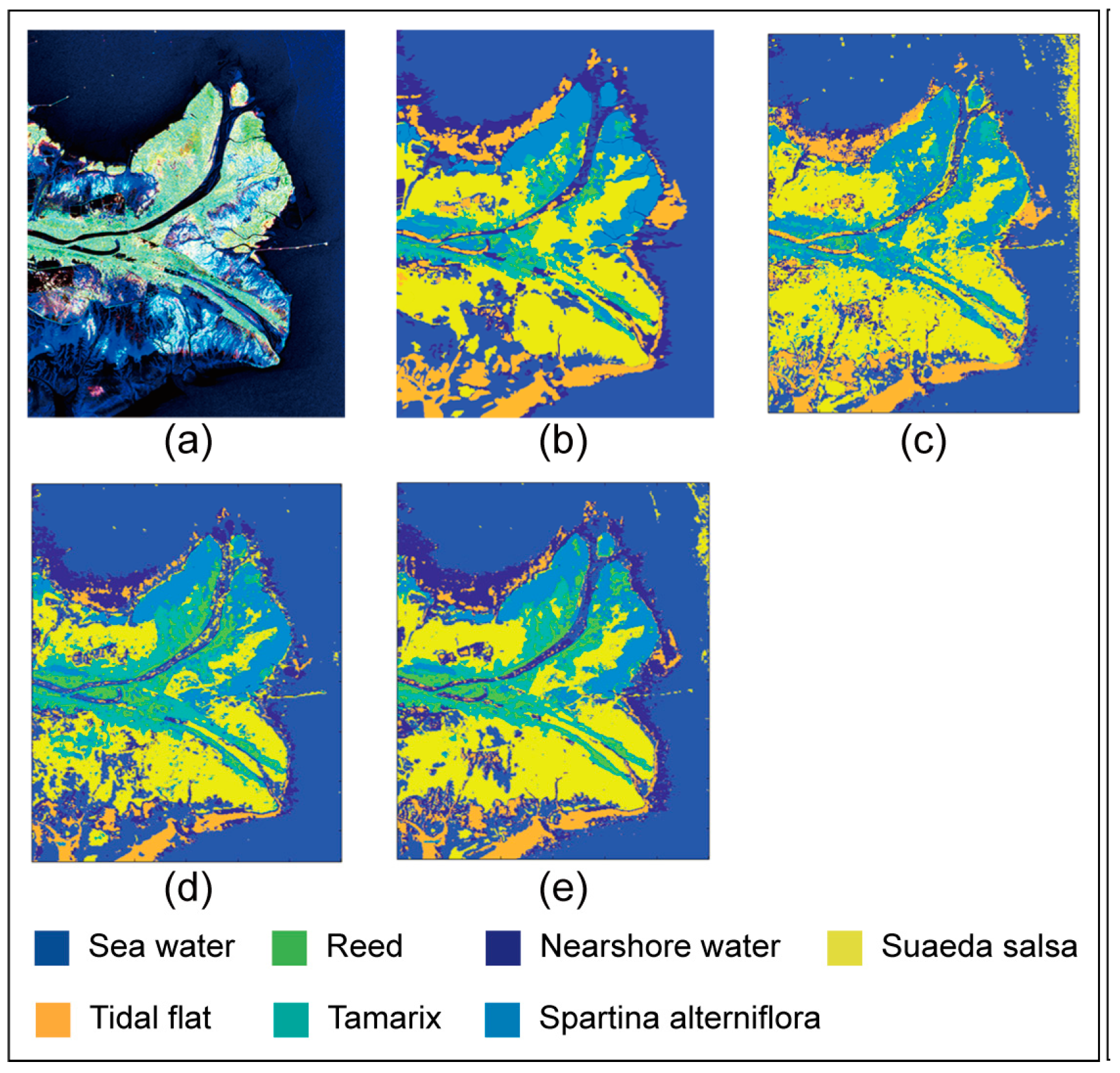
Figure 7.
The classification results of the three research schemes on AlexNet. GF-3 Data (a) Pauli pseudo color map. (b) Ground truth map. Classifification results of (c) schem1. (d) schem2. (e) schem3.
Figure 7.
The classification results of the three research schemes on AlexNet. GF-3 Data (a) Pauli pseudo color map. (b) Ground truth map. Classifification results of (c) schem1. (d) schem2. (e) schem3.
3.3. Classification Results of the Yellow River Delta on VGG16
Meanwhile, on VGG16, verification tests were conducted on the three data input schemes. Similar to the testing results on AlexNet, when using VGG16 to test three data input schemes, there are still situations where the classification accuracy of certain land objects is low. Overall, scheme 3 showed better classification performance than the other two schemes. Except for reeds and tidal flats, the classification accuracy of the other five land cover types remained consistently high. At the same time, the highest overall classification accuracy and average overall classification accuracy are also superior to the other two schemes, indicating that scheme 3 had relatively more complete polarization information prior to inputting it into the network model. Scheme 2 slightly underperformed scheme 3 in the classification accuracy of suaeda salsa, with an accuracy of only 66.2%. Particularly, scheme 2 struggled to classify tidal flats well, with a classification accuracy of only 28.5%. For scheme 1, the overall land cover classification accuracy was lower compared to the other two schemes, mainly due to the limited number of polarimetric feature parameters, which failed to effectively represent the classified area in the input network model. The specific classification accuracies are shown in Table 4.
4. Conclusion
In this paper, a deep learning-based classification scheme for PolSAR image using polarimetric scattering features is proposed through rigorous mathematical derivation. This scheme utilizes the combination of polarimetric power features, ensuring that each channel represents power values and is equivalent to other channels. Each channel possesses practical physical meanings and clear mathematical significance. Experimental results demonstrate that compared to the 6-parameter and 4-parameter data input schemes, the proposed scheme has more comprehensive information and achieves higher classification accuracy. The proposed scheme is validated on the GF-3 dataset and shows performance improvement. However, for the classification of certain land objects, this approach lacks sufficient accuracy and there are situations where the information is not comprehensive enough.
In future work, more comprehensive data input schemes will be explored.
Acknowledgments
We would like to thank the National Satellite Ocean Application Center for providing the Gaofen-3 data. Currently, this data is available to the public, and the data access address is: https://osdds.nsoas.org.cn/.
References
- Lee, J.S.; Grunes, M.R.; Pottier, E. Quantitative comparison of classification capability: Fully polarimetric versus dual and single-polarization SAR. IEEE Trans. Geosci. Remote Sens. 2001, 39, 2343–2351. [Google Scholar]
- Wang, Y.; Cheng, J.; Zhou, Y.; Zhang, F.; Yin, Q. A multichannel fusion convolutional neural network based on scattering mechanism for PolSAR image classification. IEEE Geoscience and Remote Sensing Letters 2022, 19, 1–5. [Google Scholar] [CrossRef]
- Wang, Nengyuan Pi, Yiming. PolSAR image classification based on deep polarimetric feature and contextual information. Journal of Applied Remote Sensing 2019, 13.
- Dong, H.; Zhang, L.; Lu, D.; Zou, B. Attention-based polarimetric feature selection convolutional network forPolSAR image classification. IEEE Geoscience and Remote Sensing Letters 2022, 19, 1–5. [Google Scholar] [CrossRef]
- Lonnqvist, A.; Rauste, Y.; Molinier, M.; Hame, T. Polarimetric SAR data in land cover mapping in boreal zone. IEEE Trans. Geosci. RemoteSens. 2010, 48, 3652–3662. [Google Scholar] [CrossRef]
- McNairn, H.; Shang, J.; Jiao, X.; Champagne, C. The contribution of ALOS PALSAR multipolarization and polarimetric data to crop classification. IEEE Trans. Geosci. Remote Sens. 2009, 47, 3981–3992. [Google Scholar] [CrossRef]
- Qi, Z.; Yeh, A.G.-O.; Li, X.; Lin, Z. A novel algorithm for land use and land cover classification using RADARSAT-2 polarimetric SAR data. Remote Sens. Environ. 2012, 118, 21–39. [Google Scholar] [CrossRef]
- Cloude, S.R.; Pottier, E. A review of target decomposition theorems in radar polarimetry. IEEE Trans. Geosci. Remote Sens. 1996, 34, 498–518. [Google Scholar] [CrossRef]
- Cloude, S.R.; Pottier, E. An entropy based classification scheme for land applications of polarimetric SAR. IEEE Trans. Geosci. Remote Sens. 1997, 35, 68–78. [Google Scholar] [CrossRef]
- Lardeux, C.; et al. Support vector machine for multifrequency SAR polarimetric data classification. IEEE Trans. Geosci. Remote Sens. 2009, 47, 4143–4152. [Google Scholar] [CrossRef]
- Dickinson, C.; Siqueira, P.; Clewley, D.; Lucas, R. Classification of forest composition using polarimetric decomposition in multiple landscapes. Remote Sens. Environ. 2013, 131, 206–214. [Google Scholar] [CrossRef]
- Lee, J.-S.; et al. Unsupervised classification using polarimetric decomposition and the complex Wishart classifier. IEEE Trans. Geosci.Remote Sens. 1999, 37, 2249–2258. [Google Scholar]
- Silva, W.B.; Freitas, C.C.; Sant’Anna, S.J.S.; Frery, A.C. Classification of segments in PolSAR imagery by minimum stochastic distances between Wishart distributions. IEEE J. Sel. Topics Appl. Earth Observ. Remote Sens. 2013, 6, 1263–1273. [Google Scholar] [CrossRef]
- Chen, Q.; Kuang, G.Y.; Li, J.; Sui, L.C.; Li, D.G. Unsupervised land cover/land use classification using PolSAR imagery based on scattering similarity. IEEE Trans. Geosci. Remote Sens. 2013, 51, 1817–1825. [Google Scholar] [CrossRef]
- Wu, Y.H.; Ji, K.F.; Yu, W.X.; Su, Y. Region-based classification of Polarimetric SAR imaged using Wishart MRF. IEEE Trans. Geosci.Remote Sens. Lett. 2008, 5, 668–672. [Google Scholar] [CrossRef]
- Liu, B.; et al. Superpixel-based classification with an adaptive number of classes for polarimetric SAR images. IEEE Trans. Geosci. Remote Sens. 2013, 51, 907–924. [Google Scholar] [CrossRef]
- Cloude, S.R.; Pottier, E. A review of target decomposition theorems in radar polarimety [J]. IEEE TGRS 1996, 34, 498–518. [Google Scholar]
- Krogager, E. New decomposition of the radar target scattering matrix [J]. Electronics Letters 1990, 26, 1525–1527. [Google Scholar] [CrossRef]
- Freeman, A.; Durden, S.L. A three-component scattering model for polarimetric SAR data. IEEE Trans. Geosci. Remote Sensing l998, 36, 963–973. [Google Scholar] [CrossRef]
- Yoshio Yamaguchi. Four-component scattering model for polarimetric SAR image decomposition. IEEE Trans. Geosci. Remote Sensing 2005, 43, 1699–l706. [Google Scholar] [CrossRef]
- W T, A.; Lin, M.S. A reflection symmetry approximation of multi-look polarimetric SAR data and its application to freeman-durden decomposition[J]. IEEE Transactions on Geoscience & Remote Sensing 2019, 57, 3649–3660. [Google Scholar]
- Freeman, A.; Durden, S.L. A three-component scattering model for polarimetric SAR data. IEEE Trans. Geosci. Remote Sens. 1998, 36, 963–973. [Google Scholar] [CrossRef]
- van Zyl, J.J.; Arii, M.; Kim, Y. Model-based decomposition of polarimetric SAR covariance matrices constrained for nonnegative eigenvalues. IEEE Trans. Geosci. Remote Sens. 2011, 49, 3452–3459. [Google Scholar] [CrossRef]
- Cloude, S.R.; Pottier, E. An entropy based classification scheme for land applications of polarimetric SAR. IEEE Trans. Geosci. Remote Sens. 1997, 35, 68–78. [Google Scholar] [CrossRef]
- Huynen, J.R. Physical reality of radar targets. Proc. SPIE 1993, 1748, 86–96. [Google Scholar]
- Cameron, W.L.; Leung, L.K. Feature motivated polarization scattering matrix decomposition. in Proc. IEEE Int. Conf. Radar, vol. 1, May 1990, pp. 549–557. 19 May.
- Krogager, E. New decomposition of the radar target scattering matrix. Electron. Lett. 1990, 26, 1525–1527. [Google Scholar] [CrossRef]
- Nie, W.; Huang, K.; Yang, J.; Li, P. A deep reinforcement learning-based framework for PolSAR imagery classification. IEEE Transactions on Geoscience and Remote Sensing 2022, 60, 1–15. [Google Scholar] [CrossRef]
- Wang, Y.; Cheng, J.; Zhou, Y.; Zhang, F.; Yin, Q. A multichannel fusion convolutional neural network based on scattering mechanism for PolSAR image classification. IEEE Geoscience and Remote Sensing Letters 2022, 19, 1–5. [Google Scholar] [CrossRef]
- Ren, B.; Zhao, Y.; Hou, B.; Chanussot, J.; Jiao, L. A mutual information-based self-supervised learning model for PolSAR land cover classification. IEEE Transactions on Geoscience and Remote Sensing 2021, 59, 9224–9237. [Google Scholar] [CrossRef]
- Hinton, G.E.; Osindero; Teh, Y.-W. A fast learning algorithm for deep belief nets. Neural Comput. 2006, 18, 1527–1554. [Google Scholar]
- Vincent P; Larochelle H; Lajoie I; Bengio Y, Manzagol P-A. Stacked denoising autoencoders: Learning useful representations in a deep network with a local denoising criterion. J. Mach. Learn. 2010, 11, 3371–3408.
- Goodfellow, I.; Pouget-Abadie, J.; Mirza, M.; Xu, B.; Warde-Farley, D.; Ozair, S.; Courville, A.; Bengio, Y. Generative adversarial networks. Communications of the ACM 2020, 63, 139–144. [Google Scholar] [CrossRef]
- Krizhevsky, A.; Sutskever, I.; Hinton, G.E. ImageNet Classification with Deep Convolutional Neural Networks. In Proceedings of the 25th international conference on neural information processing systems, Lake Tahoe, NV, USA, 3–6 December 2012; pp. 1097–1105. [Google Scholar]
- Szegedy, C.; Liu, W.; Jia, Y.; Sermanet, P.; Reed, S.; Anguelov, D.; Erhan, D.; Vanhoucke, V.; Rabinovich. A going deeper with convolutions. In Proceedings of the IEEE Conference on Computer Vision and Pattern Recognition (CVPR), Boston, MA, USA, 7–12 June 2015. [Google Scholar]
- Jiao, L.; Liu, F. Wishart deep stacking network for fast POLSAR image classifification. IEEE Trans. Image Process. 2016, 25, 3273–3286. [Google Scholar] [CrossRef] [PubMed]
- Liu, F.; Jiao, L.; Tang, X. Task-oriented GAN for PolSAR image classifification and clustering. IEEE Trans. Neural Netw. Learn. Syst. 2019, 30, 2707–2719. [Google Scholar] [CrossRef] [PubMed]
- Guo, Y.; Wang, S.; Gao, C.; Shi, D.; Zhang, D.; Hou, B. Wishart RBM based DBN for polarimetric synthetic radar data classifification. In Proceedings of the IEEE Int. Geosci. Remote Sens. Symp. (IGARSS); 2015. [Google Scholar]
- Shao, Z.; Zhang, L.; Wang, L. Stacked sparse autoencoder modeling using the synergy of airborne LiDAR and satellite optical and SAR data to map forest above-ground biomass. IEEE J. Sel. Topics Appl. Earth Observ. 2017, 10, 5569–5582. [Google Scholar] [CrossRef]
- Zhang, L.; Ma, W.; Zhang, D. Stacked sparse autoencoder in PolSAR data classifification using local spatial information. IEEE Geosci. Remote Sens. Lett. 2016, 13, 1359–1363. [Google Scholar] [CrossRef]
- Yu, Y.; Li, J.; Guan, H.; Wang, C. Automated detection of three-dimensional cars in mobile laser scanning point clouds using DBM-Hough-forests. IEEE Trans. Geosci. Remote Sens. 2016, 54, 4130–4142. [Google Scholar] [CrossRef]
- Chen, Y.; Lin, Z.; Zhao, X.; Wang, G.; Gu, Y. Deep learning-based classifification of hyperspectral data. IEEE J. Sel. Topics Appl. Earth Observ. Remote Sens. 2014, 7, 2094–2107. [Google Scholar] [CrossRef]
- Zhang, L.; Shi, Z.; Wu, J. A hierarchical oil tank detector with deep surrounding features for high-resolution optical satellite imagery. IEEE J. Sel. Topics Appl. Earth Observ. Remote Sens. 2015, 8, 4895–4909. [Google Scholar] [CrossRef]
- Liang, H.; Li, Q. Hyperspectral imagery classifification using sparse representations of convolutional neural network features. Remote Sens. 2016, 8, 99. [Google Scholar] [CrossRef]
- Yu, Y.; Li, J.; Guan, H.; Jia, F.; Wang, C. Learning hierarchical features for automated extraction of road markings from 3-D mobile LiDAR point clouds. IEEE J. Sel. Topics Appl. Earth Observ. Remote Sens. 2015, 8, 709–726. [Google Scholar] [CrossRef]
- Xie, H.; Wang, S.; Liu, K.; Lin, S.; Hou, B. Multilayer feature learning for polarimetric synthetic radar data classifification. in Proc. IEEE IGARSS, Jul. 2014, pp. 2818–2821.
- Huynen, J.R. Physical reality of radar targets. Proc. SPIE 1993, 1748, 86–96. [Google Scholar]
- Chen, X.; Hou, Z.; Dong, Z.; He, Z. Performance analysis of wavenumber domain algorithms for highly squinted SAR. IEEE Journal of Selected Topics in Applied Earth Observations and Remote Sensing 2023, 16, 1563–1575. [Google Scholar] [CrossRef]
- Wang, J.A.F.; Mao, Y.; Luo, Q.; Yao, B. A fine PolSAR terrain classification algorithm using the texture feature fusion-based improved convolutional autoencoder. IEEE Transactions on Geoscience and Remote Sensing 2022, 60, 1–14. [Google Scholar] [CrossRef]
- Zhou, Y.; Wang, H.; Xu, F.; Jin, Y.-Q. Polarimetric SAR image classifification using deep convolutional neural networks. IEEE Geosci. Remote Sens. Lett. 2016, 13, 1935–1939. [Google Scholar] [CrossRef]
- Chen, S.-W.; Tao, C.-S. PolSAR image classifification using polarimetric-feature-driven deep convolutional neural network. IEEE Geosci. Remote Sens. Lett. 2018, 15, 627–631. [Google Scholar] [CrossRef]
- An, W.; Lin, M.; Yang, H. Modified reflection symmetry decomposition and a new polarimetric product of GF-3. IEEE Geoscience and Remote Sensing Letters 2022, 19, 1–5. [Google Scholar] [CrossRef]
- An, Wentao. Polarimetric decomposition and scattering characteristic extraction of polarimetric SAR. Ph.D. Dissertation, Tusinghua University, Beijing, China, 2010. [Google Scholar]
- Yang, J. On Theoretical Problems in Radar Polarimetry. Ph.D Dissertation, Niigata University, Niigata, Japan, 1999. [Google Scholar]
- User Manual of Gaofen-3 Satellite Products, China Resources Satellite Application Center, 2016.
- Chen, J.; Chen, Y.L.; An, W.T.; Cui, Y.; Yang, J. Nonlocal filtering for polarimetric SAR data: A pretest approach. IEEE Trans. Geosci. Remote Sens. 2011, 49, 1744–1754. [Google Scholar] [CrossRef]
- Zhang, S.; An, W.; Zhang, Y.; Cui, L.; Xie, C. Wetlands Classification Using Quad-Polarimetric Synthetic Aperture Radar through Convolutional Neural Networks Based on Polarimetric Features. Remote Sens. 2022, 14, 5133. [Google Scholar] [CrossRef]
 |
Shuaiying Zhang received the B.S. and M.S. degrees from the Henan Polytechnic University, Jiaozuo, China and National Marine Environmental Forecasting Center, Beijing, China in 2020 and 2023, respectively. He is pursuing the Ph.D. degree with the College of Electronic Science and Engineering, National University of Defense Technology (NUDT), Changsha, China. His research interests include PolSAR data processing and Radar image interpretation. |
 |
Lizhen Cui received the B.S. degree in environmental science from Hebei Agricultural University, China, in 2018. She is currently pursuing the Ph.D. degree with ecology at the Laboratory of Terrestrial Ecosystems, College of Life Sciences, the University of Chinese Academy of Sciences, Beijing, China since 2018. She is interested in the restoration and sustainable development of alpine grassland ecosystems. |
 |
Wentao An received the B.S. degree in communication engineering from Nankai University, Tianjin, China, in 2003, and the Ph.D. degree in electronic engineering from Tsinghua University, Beijing, China, in 2010. He is currently a Researcher with the Department of Systematic Engineering, National Satellite Ocean Application Service, Beijing. His research interests include polarimetric SAR data. |
 |
Zhen Dong was born in Anhui, China, in Sepember 1973. He received the Ph.D. degree in electrical engineering from National University of Defense Technology (NUDT), Changsha, in 2001. He is currently a Professor with the College of Electronic Science and Engineering, NUDT. His recent research interests include SAR system design and processing, Ground Moving Target Indication (GMTI), and very-high-resolution SAR imaging. |
Figure 1.
Data processing flowchart.
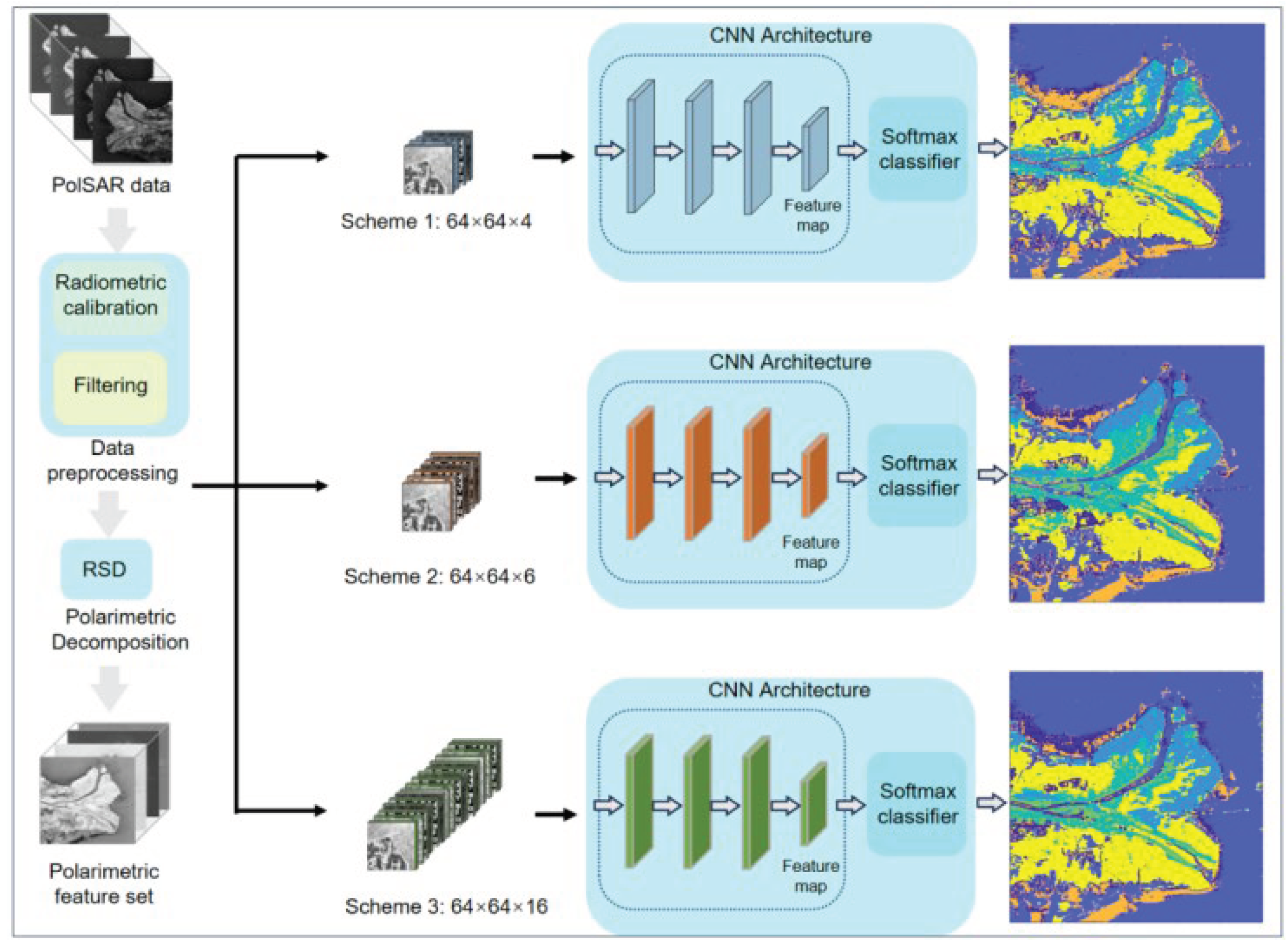
Figure 2.
Histogram of polarization feature distribution for data input scheme 1. (a) P0; (b) PS; (c) PD; (d) PV.
Figure 2.
Histogram of polarization feature distribution for data input scheme 1. (a) P0; (b) PS; (c) PD; (d) PV.
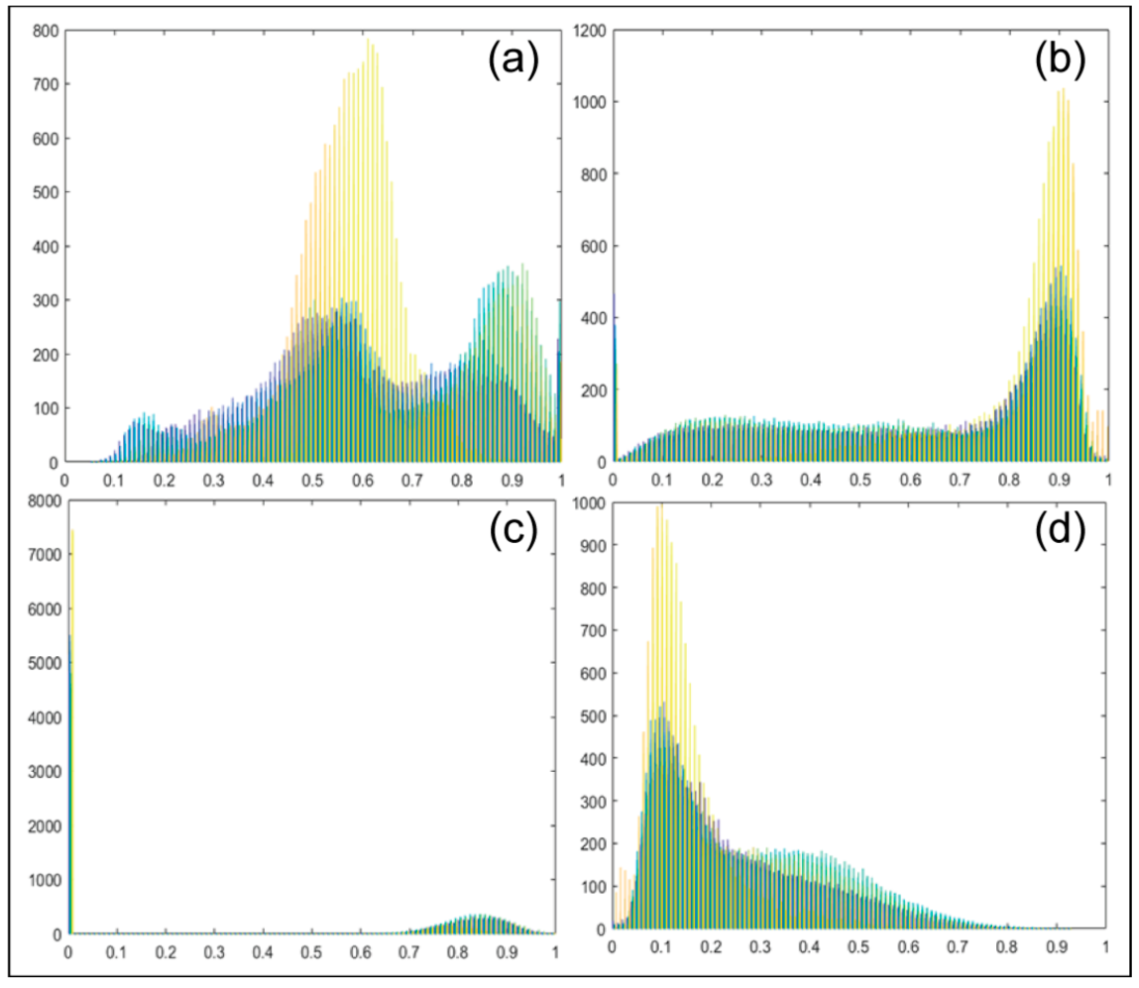
Figure 3.
Histogram of polarization feature distribution for data input scheme 2. (a) NonP0; (b) T22; (c) T33; (d) coeT12; (e)coeT13; (f) coeT23.
Figure 3.
Histogram of polarization feature distribution for data input scheme 2. (a) NonP0; (b) T22; (c) T33; (d) coeT12; (e)coeT13; (f) coeT23.
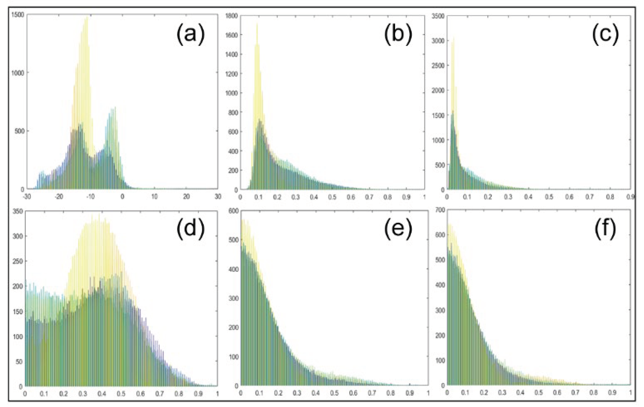
Figure 4.
Histogram of polarization feature distribution for Data Input Scheme 3. (a) P0, (b) T11, (c) T22, (d) T33, (e) H(T12), (f) H(T13), (g) H(T23), (h) L(T12), (i) L(T13), (j) L(T23), (k) V(T12), (l) V(T13), (m) V(T23), (n) R(T12), (o) R(T13), (p) R(T23).
Figure 4.
Histogram of polarization feature distribution for Data Input Scheme 3. (a) P0, (b) T11, (c) T22, (d) T33, (e) H(T12), (f) H(T13), (g) H(T23), (h) L(T12), (i) L(T13), (j) L(T23), (k) V(T12), (l) V(T13), (m) V(T23), (n) R(T12), (o) R(T13), (p) R(T23).
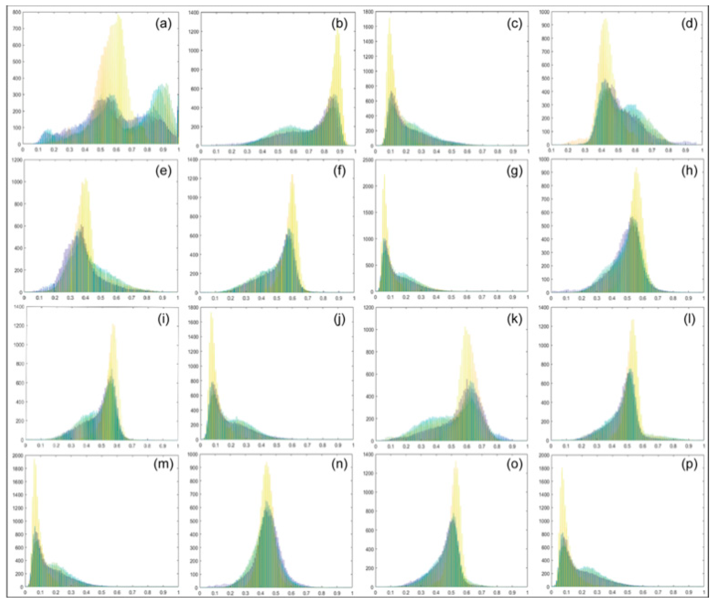
Figure 5.
Study area location and it’s corresponding image.
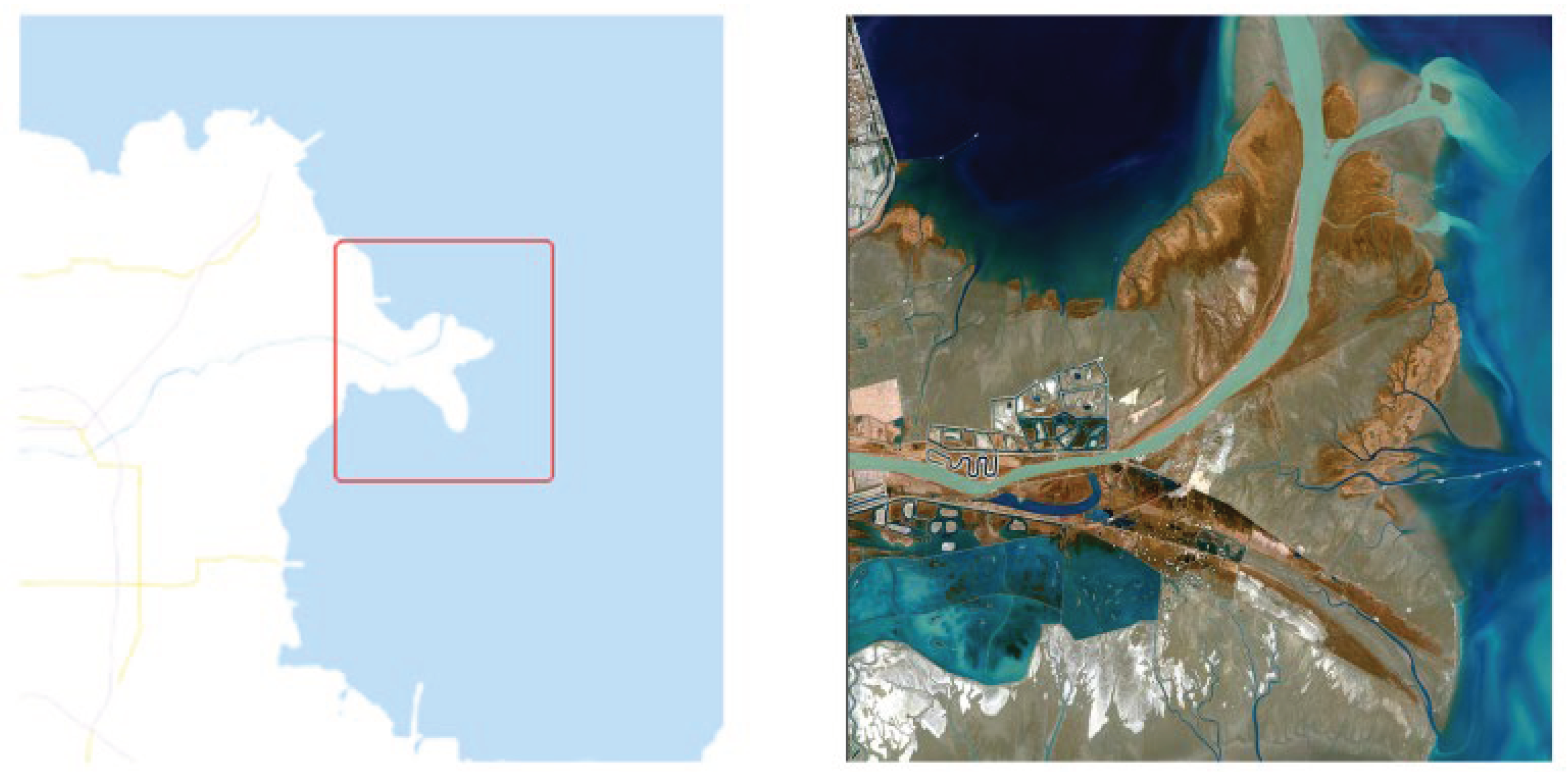
Figure 6.
UAV images of ground objects. (a) Nearshore water; (b) Seawater; (c) Spartina alterniflora; (d) Suaeda salsa; (e) Tamarix; (f) Reed; (g) Tidal flat.
Figure 6.
UAV images of ground objects. (a) Nearshore water; (b) Seawater; (c) Spartina alterniflora; (d) Suaeda salsa; (e) Tamarix; (f) Reed; (g) Tidal flat.
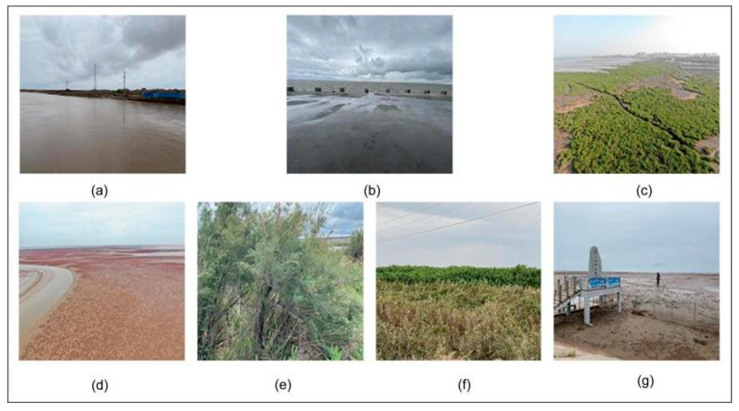
Figure 8.
Classification results of three research schemes on VGG16. GF-3 Data. (a) Pauli pseudo color map; (b) Ground truth map. Classification results of (c) schem1; (d) schem2; (e) schem3.
Figure 8.
Classification results of three research schemes on VGG16. GF-3 Data. (a) Pauli pseudo color map; (b) Ground truth map. Classification results of (c) schem1; (d) schem2; (e) schem3.
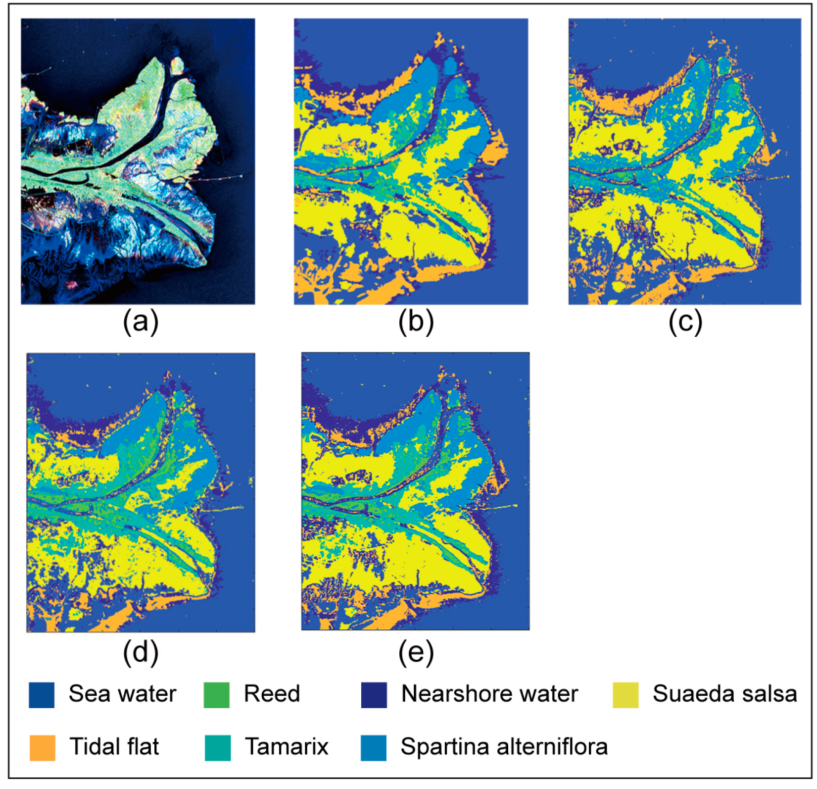

Table 1.
List of three polarization data input schemes.
| Scheme | parameters | Polarization features |
| 1 | 4 | P0, PS, PD, PV |
| 2 | 6 | NonP0, T22, T33, coeT12, coeT13, coeT23 |
| 3 | 16 | P0, T12, T23, T23, H(T12), H(T13), H(T23), L(T12), L(T13), L(T23), V(T12), V(T13), V(T23), R(T12), R(T13), R(T23) |
Table 2.
Samples distribution.
| Images | Nearshore water | Seawater | Spartina alterniflora | Tamarix | Reed | Tidal flat | Suaeda salsa |
|---|---|---|---|---|---|---|---|
| 20210914_1 | 500 | 400 | 1000 | 500 | 500 | 500 | 500 |
| 20210914_2 | 500 | 200 | 0 | 0 | 0 | 500 | 0 |
| 20211013 | 0 | 400 | 0 | 500 | 500 | 0 | 500 |
| Total | 1000 | 1000 | 1000 | 1000 | 1000 | 1000 | 1000 |
Table 3.
The classification accuracy of there polarization input schemes on AlexNet.
| Classification accuracy Input scheme |
1 | 2 | 3 |
| Nearshore water | 83.4 | 96.8 | 100 |
| Seawater | 98.7 | 96.9 | 99.60 |
| Spartina alterniflora | 87.0 | 96.8 | 93.3 |
| Tamarix | 40.1 | 100 | 100 |
| Reed | 50.4 | 94.5 | 68.50 |
| Tidal flat | 61.8 | 49.3 | 44.6 |
| Suaeda salsa | 98.2 | 50.8 | 96.8 |
| Indepent experiments Overall Accuracy | 74.23 | 83.59 | 86.11 |
| 71.36 | 81.41 | 81.53 | |
| 70.41 | 77.83 | 77.04 | |
| 68 | 73.66 | 73.73 | |
| 67.84 | 68.87 | 71.99 | |
| Average Overall Accuracy | 70.368 | 77.072 | 78.08 |
| Kappa coefficient | 0.6993 | 0.8085 | 0.8380 |
Table 4.
The classification accuracy of there polarization input schemes on VGG16.
| Classification accuracy Input scheme |
1 | 2 | 3 |
| Nearshore water | 89.3 | 95.7 | 95.6 |
| Seawater | 99.4 | 97.7 | 99.7 |
| Spartina alterniflora | 87.6 | 96.6 | 95.9 |
| Tamarix | 40.2 | 98.5 | 100 |
| Reed | 26.1 | 93.8 | 44.7 |
| Tidal flat | 73.2 | 28.5 | 58.3 |
| Suaeda salsa | 100 | 66.2 | 94.1 |
| Indepent experiments overall accuracy | 73.69 | 82.43 | 84.04 |
| 72.8 | 82.21 | 83.57 | |
| 69.7 | 81.44 | 82.07 | |
| 68.66 | 79.44 | 81.54 | |
| 67.6 | 77.53 | 80.11 | |
| Average overall accuracy | 70.49 | 80.61 | 82.266 |
| Kappa coefficient | 0.6930 | 0.7950 | 0.8138 |
Disclaimer/Publisher’s Note: The statements, opinions and data contained in all publications are solely those of the individual author(s) and contributor(s) and not of MDPI and/or the editor(s). MDPI and/or the editor(s) disclaim responsibility for any injury to people or property resulting from any ideas, methods, instructions or products referred to in the content. |
© 2024 by the authors. Licensee MDPI, Basel, Switzerland. This article is an open access article distributed under the terms and conditions of the Creative Commons Attribution (CC BY) license (http://creativecommons.org/licenses/by/4.0/).
Copyright: This open access article is published under a Creative Commons CC BY 4.0 license, which permit the free download, distribution, and reuse, provided that the author and preprint are cited in any reuse.


