
Submitted:
01 April 2024
Posted:
02 April 2024
You are already at the latest version
Abstract
Preventive Maintenance (PM) is a periodic maintenance strategy, which has great results for devices in extending their life, increasing productivity, and most importantly, help avoid unexpected breakdowns and their costly consequence. A preventive maintenance scheduling (PMS) is determining the time for carrying out PM, and it represents a sensitive issue in terms of impact on production if the time for the PM process is not optimally distributed. In this study, hybrid heuristic methods were used to solve the PMS problem, as genetic algorithm and Tabu research were adopted. The optimal solution was reached in a short time compared to previous studies in which optimal methods were used, integer programming and nonlinear integer programming. Also, sensitivity analysis was applied to measure the robustness and strength of the method used, where an optimal solution was obtained for all experiments and in record time. This method can be used for power plants in privet or public sectors, to generate an optimal PMS, to save money, and to avoid water or electricity cuts.
Keywords:
preventive maintenance
; scheduling
; optimization
; genetic algorithm
; tabu search
; metaheuristic
1. Introduction
The maintenance of all kinds of equipment or machinery plays an important role in protecting it from sudden breakdowns that may cause halting or delaying production, especially for essential matters for consumers. It also improves uptime and extends its operational life. The main objective of maintenance is to ensure that all equipment required for production is operating efficiently at all times. With the development of science, several maintenance strategies have emerged. There are many types of maintenance strategy, where the most commonly used are; Reactive maintenance (run-to-fail), which relies on the technique of using things until they break before they can be fixed. Predetermined Maintenance is another strategy, which simply follows the manufacturer's recommendations for maintenance, including when to perform checks and maintenance. Another type of maintenance strategy is predictive maintenance, which is based on data and indicators of the current actual condition of the equipment, through which the maintenance process is carried out. The most widely used type of maintenance technique is preventive maintenance PM, where in 2020 according to [1], 76% of companies in the manufacturing industry worldwide prioritized PM. This technique relies on performing a regularly and routine scheduled maintenance (PMS) to fix small problems before they develop into major problems, Figure 1 illustrated the workflow of PM. For more details about maintenance strategies in general, see [2,3].
There are many benefits of PM such as; extending the life of assets, reduce the risk of breakdowns, increases efficiency, minimize unplanned downtime, increase customer satisfaction, etc. see [5]. Many different sectors apply PM in their sector, for example; in the field of transportation; vehicles [6,7], aircraft [8,9], trains [10,11], and ships [12]. In the field of factories or stations [13,14,15,16,17,18], other sectors [19,20,21,22,23].
Power plants are important sectors for humanity. The main task is to provide people with electricity and fresh water. Any interruption of water or electricity has a significant negative impact. The primary goal of power stations is to produce electricity and water for consumers, so these stations are important and sensitive as they produce the necessities of life. Therefore, workers in power stations are aware of the importance of maintaining all assets and components of the station, in order to ensure that electricity and water are not interrupted by consumers.
A lot of research has been done in PMS, some researchers have adopted the exact optimization approach to find the optimal solution, others have resorted to using heuristic methods, for large scale problems, and others merging the two approaches. In the exact optimization approaches, Mollahassani-pour et al [24] designed Mixed Integer Linear Programming (MILP) as a framework to address PMS of power generation units. The aim of this study was to reduce the cost of maintenance while determining the most appropriate maintenance scheme. To prove the effectiveness of the proposed structure, IEEE Reliability Testing System (RTS) was used, with promising results. Al-Hamad et al. [25] provided a paper for PMS on a real case study of 32-unit system of boilers, turbines and distillers for power plants in the State of Kuwait. The problem is formulated as a Mathematical Program (MP) that increases minimum output to demand ratios, for a period of 52 weeks. All constraints were considered, and the results of the proposal were optimal compared to the schedule of power station experts, and in reasonable time. Also, Al-Hamad et al. [26] used nonlinear integer programming (NLIP) method to address the previous problem. They applied the comparison with the results obtained with the previous study in terms of the time taken to reach the optimal solution, as the time taken was reasonably higher. Fetanat and Shafipour [27] used the Ant Colony Optimization for Continuous Domains (ACOR) to treat the problem of unit maintenance scheduling, as the aim of this study was to reduce cost and reliability. Constraints such as rotational reserve and maintenance crew duration were taken into account. The performance of the technique used was benchmarked against those reported in the literature, and the method that was used proved to be superior to them in terms of optimal resolution and speed. Canto [28] used mixed Integer Linear Programming 0/1 in order to create a schedule that allows efficient organization of preventative maintenance over a specific time horizon. The study was applied to a power plant in Spain and reliability is the main point used in the presented methodology.
Since exact optimization algorithms take a long time to reach the optimal solution, moreover, it is difficult to find an optimal solution as the dimensions of the system increase, so many researchers resort to using heuristics methods to solve large scale problems. Lapa et al. [29] used Genetic Algorithms (GA) technology in the PM of the power plant. Some relevant features have been taken into account, for example: possibility of needing repair, cost of repair, and possibility of incomplete maintenance. Pressurized water reactors (PWR) were applied as a case study, and the results were good. Alimohammadi and Behnamian [30] presented a study aimed at scheduling the PM of a group of feeders in the Electricity Distribution Company of Iran, where mathematical programming was proposed for this problem. During the study, two heuristic algorithms were provided with the aim of providing a good solution in a reasonable time. The results of the proposed algorithms were validated as the results of the heuristic algorithms were very suitable. Dahal and Chakpitak [31] used a hybrid genetic algorithm (GA), simulated annealing (SA) to schedule preventive generator maintenance. The results were promising and showed that the use of hybrid methods provides an effective alternative to solve this type of problem. Duarte et al. [32] adopted particle swarm optimization (PSO) and genetic algorithms (GA) for PMS in the Cuban power system. The goal is to reduce the risk of load loss as much as possible in the power system. The paper demonstrates the effectiveness of the proposed model in this real power system. For more literature review in this field of PMS optimization, and applications to power plants, see [33,34].
The method adopted to address this problem was implemented through two indicative mixed methods, the genetic algorithm GA and the tabu search TS. GA and TS are a metaheuristic problem-solving approach used to solve combinatorial optimization problems. GA was developed by John Holland and his collaborators in the 1960s and 1970s [35,36], while TS was proposed in 1989 by Fred Glover of TAPO Research [37]. In a GA, the basic elements are chromosome representation, fitness selection, and biologically inspired factors. A set of solutions, called a population, which is randomly or scientifically generated. Each population consists of a number of chromosomes, and in each chromosome a set of genes. Each gene locus on the chromosomes is usually represented in binary format, or as a set of integers, depending on the type of problem. Fitness represents the chromosome value, where the best objective function value is searched, through a number of iterations to improve the solution. The process is carried out by a group of parents who must be selected in order to find a new solution by applying two factors: crossover and mutation method. The process continues by selecting the best parents from among the population, with the aim of reproducing a new generation with different characteristics. The process of reproduction of offspring in the next generations takes place through the evolutionary algorithm, which is inspired by the theory of crossover and mutation. Crossover is mainly used to create new solutions from the genetic information of a population, while mutation occurs to bring in new information and diversity within the population and move away from early convergence to make the solution more general. This process will be repeated for a number of iterations until an optimal or near optimal solution is found.
Tabu Search (TS) is a metaheuristic search method that uses local search methods. The search method is developed by making it move from the local area to the global area, which discourages the search for previously visited solutions. The search starts from the possible solution x to the optimal solution x' near x, until the stopping criterion, which is the number of iterations mentioned, is reached, or the desired solution (score threshold) is reached. Two operators, swap and insert, are applied during the search. Solutions are sought in the current region extensively (intensification), but usually after a number of iterations, the solutions are suboptimal or discouraging. To discourage the algorithm from revisiting solutions that have already been explored recently, “Tabu list” is applied. Tabu List is a short-term compilation of solutions visited in the recent past. This solution remains "tabu" or forbidden for a number of tn “tabu tenure”. Tabu tenure tn refers to the duration or number of iterations for which a solution or move remains on the Tabu List. It's a way to control how long a particular choice is considered "tabu" or forbidden. This mechanism encourages diversification by preventing the search from getting stuck in local optima or repetitive cycles. As the algorithm explores new solutions, it increases the likelihood of discovering a broader range of possibilities, leading to a more diverse and thorough search for the optimal solution. Aspiration Criteria, one the other hand, provide exception based on specific criteria to excluding the best solution from the tabu list, the algorithm remains free to explore the neighborhood of that solution, potentially finding even better solutions in the same region. These criteria could be based on improvements in the objective function, reaching a specific threshold, or satisfying other relevant conditions, whereas in this research they are based on achieving the best solution so far. This helps balance exploration and exploitation in the search process.
This study will focus on the power plant in the State of Kuwait, this station that contains turbines, boilers, and distillers. The main goal is to schedule preventive maintenance equipment in a way that maximizes equipment utilization while minimizing power outages. A hybrid Genetic Algorithm and Tabu Search would be the methodology to tackle this problem, as the study provides the PMS for each piece of equipment in the power plant, for time period of 12 months. The results will be compared with the results of the previous optimization approaches [25,26] in order to measure the quality of this methodology, in terms of solution quality and implementation time. Certain constraints will be taken into account, such as maintenance window restrictions, maintenance duration for each equipment, the level of reservoir water limits, etc. The positive effects of this study are to meet consumer demands without any shortage or interruption, whether for water or electricity. In addition to maintaining equipment for a long time without any breakdown that leads to expensive repairs.
2. Problem Description
2.1. Problem Background
The current study will focus on power plants in the State of Kuwait. Power plants generally consist of a number of stations, each station containing three type of equipment, turbines, boilers, and distillers. The energy production process in the power stations in Kuwait takes place by drawing sea water, which is first transferred to the boilers, in order to heat up to produce high-pressure steam. The steam is then transmitted to two paths, to the distillers, in order to condense and get rid of the salt, to produce drinking water. The other is transmitted to the turbines in order to produce electricity. To continue producing energy and provide the citizens’ needs for electricity and water without interruption, the plant needs annual PM. Station consists of a number of plants, p Each plant consists of different numbers of distillers , turbines , and boilers . The maintenance time period T for all equipment in the station is within a full year, 52 weeks. Each piece of equipment in the plant needs a number of weeks to complete the PM process.
2.2. Problem Formulation
Research manuscripts reporting large datasets that are deposited in a publicly available database should specify where the data have been deposited and provide the relevant accession numbers. If the accession numbers have not yet been obtained at the time of submission, please state that they will be provided during review. They must be provided prior to publication.
The nomenclature for the hybrid GA and TS approach was divided into sets, data, and decision variables, as follows:
Sets:
(The sequence of genes in the chromosome represents the sequence of weeks in time horizon)
Data:
.
.
.
At , where are the minimum and maximum water level at the reservoir.
Decision variable:
There are 3 types of decision variables, first, binary variables:
During the boiler maintenance period, the distillers and turbines will be either under maintenance or idle, until the boiler maintenance is completed. The following binary variables express this situation:
Second, integer variables:
2.3. Hybrid Approach
The proposed approach is implemented by hybrid GA and TS. The process begins with applying first a GA, which consists of a set of strips, each strip is called a chromosome or solution, and each chromosome consists of a set of variables known as genes. The set of chromosomes is called the population.
The basis of the proposed approach is to produce populations over iterations, where each population across iterations consists of a set of chromosomes. Each chromosome represents PMS for all equipment in the station, as illustrated in Figure 2
Each chromosome consists of a group of genes, which represents the sequence of weeks in a year. The value for each gene represented by gene , for parent represents one of the equipment under PM. Simply, a chromosome consists of a sequence of genes (subsequences) which means this equipment is subject to PM, while an empty gene means no PM during this week. For example, as shown in Figure 3, means that equipment 6 is under maintenance in week 1, while means that equipment 2 is under maintenance in week i. In addition, , represent the maintenance duration time for equipment q, in plant p. So, for example, means, equipment 6 needs three weeks to complete PM (from week 1 to week 3), while means that equipment 7 needs four weeks to complete PM, as shown in Figure 3.
Next, the fitness function score of all chromosomes in the population is determined. The degree of fitness function increases the likelihood that it will be selected for producing new offspring. The best the fitness score, the higher the chances of reproductive selection. Before calculating the fitness function, the gap between energy demand and availability must be calculated. There are two types of gaps, as shown below:
where is the gap of distillers between production of water and water demand , at gene , (which represents week as mentioned previously). Likewise, is the gap of turbines, between available production of electricity and electricity demand , at gene .
The fitness function for each parent consists of two standard deviations, one for distillers production where represents the average gap of water production and demand across the time horizon, and the other for turbines production where represents the average gap of electricity production and demand across the time horizon.
These two are calculated separately, provided that the fitness value of both is the smallest in the same chromosome. Whenever the value of the fitness function is very small, this indicates that the gap between demand and available production will be approximately the same over the time horizon. This means that there is very little chance of power or water supply being cut off. Therefore, two different parents will be selected, one with the smaller standard deviation for water production , while the other parent with the smaller standard deviation for electricity production The algorithm uses two operators that are applied to the two selected parents, crossover and mutation. The traditional method in the GA to select cut points is done randomly, but here it is implemented in a scientific way. The method begins by selecting a non-empty gene in parent 1, such that the gap for that gene is the smallest throughout the chromosome. For example, as shown in Figure 4, the gene with value 6 (equipment number 6) is selected. Likewise, for parent 2, the gene with the same value as parent 1, which is equipment number 6. The maintenance duration of equipment q is represented by , where in this example, equipment 6 needs a period equal to 3 weeks to complete PM, . Therefore, all genes with the same value will be reserved for the crossover operation, the number of which is equal to .
In the next step, selecting the empty gene with the highest gap value for distillers, , for parent 1, and the same process is performed for parent 2 by selecting gene , with the highest gap for boilers, . The next step is to choose the cut points, which is done by choosing a number of genes adjacent to gene i of parent 1, so that their number is equal to the number of genes, and the same thing is done for parent 2, as shown in Figure 4 Step 2. As clear in Figure 4, the number of empty genes equals 2 genes, so any non-empty genes within the cut points will be moved outwards, either to the right or left depending on their position. For parent 1, genes of value 1 were moved one step to the right, while in parent 2, genes of value 3 were moved one step to the left, as shown in Figure 4 step 3. In the final step of the crossover process, the selected substring (genes with value 6) will be inserted between the cut points, producing new offspring with a new fitness value, as shown in Figure 4 step 4.
At this stage, the tabu list method is adopted, which is one of the features of TS, in which the selected genes, i and j, will enter two separate tabu list for a number of iterations, tenure. This property is important and helps to diversify the search and explore new regions of the solution space. At the same time, when the value of fitness to the new offspring is the best so far, aspiration criteria are applied, where the two selected genes, will be released from the tabu list. This process can actually enhance the focus and intensity of the search for promising solutions in a particular area.
The mutation operator will be applied after the crossover, Figure 5 illustrates the process. The process is done by first randomly selecting a substring of genes for both parents, as shown in Figure 5, genes with a value of 3 in P1, and genes with a value of 1 in P2. The substring is then shifted to the left or right, depending on the position of the empty gene. If there is no empty gene next to the substring, the adjacent substrings are shifted until they reach an empty gene.
This process will continue for of iterations. This means that the search in these two chromosomes has been explored in a precise and extensive manner. Next, a new population with number of chromosomes are generated, in the same manner as previous. Different parents are selected in the same way as previous, in order to search for a better solution. The algorithm will terminate after reaching the threshold fitness value. This solution will be determined as the optimal solution for the population. On the other hand, if the optimal solution is not reached, the algorithm will stop when of iterations are reached.
There are some conditions that must be followed during the process of searching for the solution, through the proposed method, which are as follows:
Condition (5) ensures that the machine undergoes PM only once during the time horizon, so that the time to start PM is within the permitted period. To guarantee the continuity of PM within the allotted time period , without interruption, condition (6) was implemented.
Constraint (7) was put in place to ensure that the number of labors during the implementation of PM for a number of equipment does not exceed the total number of labors available in the current week.
Constraints (8) and (9) were set in order to ensure the availability of electricity and water during the current week, and that there is no shortage due to PM work. On the other hand, constraint (10) guarantees that water production is within minimum and maximum water level at the reservoir.
There are technical and precautionary matters imposed by power plants administration regarding the maximum number of equipment of the same type (turbines, boilers, distillers) on which PM is permitted during the current week. Therefore, the constraint (11) was set to ensure that the permissible number is not exceeded.
The following flowchart in Figure 6. explains the process of generating a PMS for all equipment in a plant using the proposal approach.
3. Computational Results
3.1. General Data
Data were obtained from the MEW in the State of Kuwait, where there are several power plants in the State of Kuwait. In this research, Al-Zour plant was chosen. This plant consists of 8 units, each unit consisting of 4 pieces of equipment; One boiler, one turbine and two distillers. This means that there is a total of 32 pieces of equipment in the plant. PM must be performed annually for all equipment to avoid any malfunction. Each boiler needs 5 weeks to complete PM, as well as the distiller, while turbine needs 4 weeks to complete PM. Since boilers are responsible for supplying distillers with hot steam for condensation and producing fresh water, as well as turbines for producing electricity, PM of any boiler results in the associated turbine and distiller being idle until PM is completed. In addition, no more than two units can stop in the same week either due to PM or be idle due to PM work on the boiler associated with them. According to the information provided to us by the Al-Zour station administration, human resources are available in all areas of the operational planning period. The time period to start PM for all equipment is open from the first week until the end of the year.
The objective of this study is to generate a PMS for all equipment in the station, such that it maximizes the number of operating equipment throughout the time horizon. This means, in return, minimize the occurrence of water or electricity outages for consumers. This can be achieved by making the gap between available production and demand approximately equal along the time horizon.
Hybrid GA and TS algorithm was adopted to address this problem where MATLAB R2021a programming was used to solve the problem, based on DELL desktop, CoreTM i7-1065G7 CPU clocked at 1.50GHz and 16.0GHz. The time horizon in which the proposal was implemented is one year, as a year consists of 52 weeks, assuming that a month consists of 4 and 5 weeks. The reason weeks are used in this problem is because the duration of PM for any piece of equipment is calculated in weeks.
Figure 7.a and 7.b show the water and electricity demand for one year for Al-Zour plant in the state of Kuwait, where the demand appears to increase in the summer period. Table 1. illustrates the production capacity for each piece of equipment for all units in the Al-Zour plant. D1 and D2 represent distiller 1 and 2, while R represents turbine. On the other hand, MIGD, represents million imperial gallons per day, while MW, represents million watts.
The aim of this study is to generate a reliable PMS within a reasonable CPU time, such that all gaps between demand and available production in all time periods are very close throughout the year, simultaneously, all constraints are satisfied. To achieve this goal, the standard deviations and , of the gap between demand and available production for water and electricity was adopted, provided that the method presented in this paper searches for the minimum value of the standard deviations. This ensures that there are no power outages or water shortages throughout the year.
3.2. Model Validation and Analysis: Test1
Many experiments were applied to find the optimal or near optimal solution through the following factors: number of chromosomes in each population CR, general iteration, internal iteration , method of genes selection, and the value of the tenure of Tabu list. It is important to mention before starting with the details that the results of the proposal approach have been compared with the two published articles, [25] and [26] that used optimal method, IP and NLIP, for the same case.
First, regarding the population size CR, it was gradually increased from 50 to 100 parents, with 100 being the best number, as the solution was greatly improved. In addition, there was no improvement in the solution after the population size exceeded 100 parents. According to general iteration, the value of was equal to 10,000, such that the optimal solution was reached at less time than the value for all experiments, as all cases reaching the threshold fitness value. For internal iteration, 50 iterations as α value were the best. On the other hand, selecting genes from the two parents with the aim of applying crossover and mutation, two methods were examined, the first was through random selection, while the second was scientific selection. The method of scientific selection of genes has proven to be the best, as it relies on selecting the gene for which the gap between demand and available production is the highest. The scientific selection led to the optimal solution very quickly, while this was not achieved when using the random selection method. Moreover, Tabu list played a major role in the success of the gene selection process. This prevented returning to the same solution area (the cycle problem) and diversifying the research into another solution area, as reaching the optimal solution was guaranteed by its presence, while the optimal solution was not reached when dispensing with it. The best value for tenure . Table 2 summarized all values mentioned previously.
The proposed method was applied, and the optimal solution was obtained, compared to the two IP and NLIP [25,26] for the same problem. The value of the is equal to 59.6 MIGD and the value of is equal to 33519 MW, as shown in Table 3. These results were obtained in a computational time of 20 seconds. Regarding the distribution of equipment, Table 4. displays the PMS for all equipment within one year (52 weeks) for both the proposed model and MEW. First, with regard to turbines, for the Ministry's PMS, the number of weeks in which they were shut down for PM operation, or were idle due to boiler PM, exceeds the proposed PMS approach, as they were idling in weeks 32, 33, 34, 35, and 36 as shown in Table 4. Therefore, the average in the Ministry’s PMS is less than the proposed PMS average, which resulted in a change in the standard deviation . On the other hand, the minimum gap during the year in the Ministry’s project management system is equal to 101.3 MIGD, while in the proposed approach it is equal to 118.1 MIGD, and this means that there is a difference equivalent to 16.8 MIGD. As for electricity, the minimum gap during the year is in the Ministry’s PMS is equal to 110971 MW, while in the proposed approach it is equal to 124,426 MW, which means there is a difference equivalent to 13,455 MW, as shown in Table 3. This indicates that the surplus production of water and electricity through the PMS method presented in this paper exceeded the experts of the MEW by 16.58% and 12.12% respectively. It should also be emphasized that any increase in surplus production means an increase in the ability to meet demand. Furthermore, the MEW performance management system has not been settled, with service outages during week 11 and only one piece of equipment undergoing maintenance in week 47. This is undesirable as it leads to unnecessary manpower costs at the time of low peak demand. In contrast, the proposed method for PMS avoids this unnecessary overhead.
In addition to the above, all constraints have been satisfied, as shown in Table 4, where Table 4 shows the distribution of all equipment under maintenance over a period of 52 weeks. For example, no more than two pieces of equipment of a given type are under PM during any of the 52 weeks of the planning horizon. Also, when their boiler is under PM, neither the distiller nor the turbine is working.
Figure 8.a. and 8.b, demonstrate the distribution of equipment for PM through the proposed approach, and 3.a and 3.b illustrate the schedule generated by the Ministry’s administration. They display production, demand, and number of units under maintenance. They show that the number of distillers and turbines undergoing maintenance has become constant. This keeps water and electricity production constant for the first 20 weeks. While production reaches its peak and maintenance work stops when demand increases during the summer period during weeks 21 to 32, while maintenance work resumes at the end of the summer period due to the steady decline in demand. In contrast, the production surplus is greater during the winter, ensuring a large reserve level and avoiding water shortages and power outages. It is equivalent to 118.1 MIGD for water and 124.426 MW for electricity. The total production amounts to 36,321.6 MIGD of water and 17,687,040 MW of electricity.
3.3. Model Validation and Analysis: Test2
To measure the robustness and the efficiency of the hybrid method proposed in this research, 16 experiments were conducted, through which to measure the effectiveness of the proposed tool through the quality of the solutions and the computational time to reach the solution. These experiments were divided into two parts. First, the demand for water was stabilized and increased the demand for electricity so that the increase was 5%, then it was gradually increased until reached the highest possible increase percentage. The second part is the opposite: stabilizing the demand for electricity and gradually increasing the demand for water by 5% until it reached the highest possible increase rate. First, all results were optimal compared to the results of IP and NLIP optimal methods [25], [26]. Additionally, the computational time to reach the optimal solution is less in most experiments, as illustrated in Table 5.a. and 5.b. Also, in Figure 9.a. and 9.b, the curve shows how short the computational time it takes to reach the optimal solution compared to other solutions, for both experiments. Table 5.a. and 5.b, showed that the average computational time is much lower for the two sections. In the first part, when the electricity demand is stabilized, the average of the proposed hybrid method is 61 second, while for the other two tools, the computational time is 211.8 and 401 second, for IP and NLIP, respectively, as shown in Table 5.a. Also, when the demand for water is stabilized and the demand for electricity is gradually increased, the average computational time for the proposed tool is much less than the other two tools. the average of the proposed hybrid method is 55.8 second, while for the other two tools, the computational time is 216.3 and 304.9 second, for IP and NLIP, respectively, as shown in Table 5.b. Figure 10.a and 10.b also showed the differences in computational time to reach the optimal solution.
In summary, the hybrid approach consistently outperforms the IP and NLIP approaches, showing a trend of faster optimization times. Moreover, optimal methods have great difficulty in solving large-scale problems, and may sometimes be impossible, while this is not the case for heuristic methods, such as the method proposed in this paper. This helps the user in scheduling management in any power plants, to use this proposed method to create an optimal PMS for their stations and in a short computational time. This is beneficial to save money and time.
4. Conclusions
This article delves into the complex field of PMS in cogeneration plants with production operations. These plants have a dual function of generating electricity and producing water, which makes scheduling their maintenance particularly difficult due to the need to balance production requirements with PM. The researchers aim to find an ideal schedule that reduces downtime, increases production efficiency, and reduces maintenance costs. During the study, a hybrid tool consisting of metaheuristic methods was used; GA and TS. A number of constraints are taken into consideration, such as maintenance window constraints, maintenance duration for each machine, maximum tank water level, number of available labors, etc. By taking these factors into consideration, schedules were created that ensured the reliability and longevity of plant operations while meeting production goals. After using the tool proposed in this research, the optimal solution was reached compared to previous studies that used optimal solution tools. Sensitivity analysis was also applied to measure the robustness and effectiveness of the proposal, and the optimal solution was obtained in all experiments.
The research seeks to provide cogeneration plant operators with a practical tool to optimize maintenance schedules, ultimately improving operational efficiency, reducing downtime, and saving costs. This approach represents a major advance in maintenance optimization, providing valuable insights and solutions for managing the complex interplay between production and maintenance activities in industrial environments.
Conflicts of Interest
This manuscript was not submitted to, nor is under review at, another journal or other publishing venue. The authors have no affiliation with any organization with a direct or indirect financial interest in the subject matter discussed in the manuscript.
References
- 35 Latest Maintenance Statistics for 2024: Data, Adoption & Strategies - Financesonline.com.
- https://www.mrisoftware.com/blog/4-types-of-maintenance-management-strategies/.
- hpps://www.fiixsoftware.com/blog/evaluating-maintenance-strategies-select-model-asset-management/.
- Hpps:www.gofmx.com/preventive-maintenance.
- www.gofmx.com/blog/benefits-of-preventive-maintenance/.
- Joo, S.J.; Levary, R.R.; Ferris, M.E. Planning Preventive Maintenance for a Fleet of Police Vehicles Using Simulation. SIMULATION 1997, 68, 93–99. [Google Scholar] [CrossRef]
- Güner, G.G.; Sakar, C.T.; Yet, B. A Multicriteria Method to Form Optional Preventive Maintenance Plans: A Case Study of a Large Fleet of Vehicles. IEEE Trans. Eng. Manag. 2021, 70, 2153–2164. [Google Scholar] [CrossRef]
- Safaei, N.; Banjevic, D.; Jardine, A.K.S. Workforce-constrained maintenance scheduling for military aircraft fleet: a case study. Ann. Oper. Res. 2011, 186, 295–316. [Google Scholar] [CrossRef]
- Sohn, S.Y.; Yoon, K.B. Dynamic preventive maintenance scheduling of the modules of fighter aircraft based on random e ects regression model, Journal of the Operational Research Society, 2010, 61, 974–979.
- Lin, B.; Wu, J.; Lin, R.; Wang, J.; Wang, H.; Zhang, X. Optimization of high-level preventive maintenance scheduling for high-speed trains. Reliab. Eng. Syst. Saf. 2018, 183, 261–275. [Google Scholar] [CrossRef]
- Lin, B.; Zhao, Y. Synchronized optimization of EMU train assignment and second-level preventive maintenance scheduling. Reliab. Eng. Syst. Saf. 2021, 215, 107893. [Google Scholar] [CrossRef]
- Go, H.; Kim, J.-S.; Lee, D.-H. Operation and preventive maintenance scheduling for containerships: Mathe- matical model and solution algorithm, European Journal of Operational Research, 2013, 229, 626–636.
- Kamel, G.; Aly, M.F.; Mohib, A.; Afefy, I.H. Optimization of a multilevel integrated preventive maintenance scheduling mathematical model using genetic algorithm. Int. J. Manag. Sci. Eng. Manag. 2020, 15, 247–257. [Google Scholar] [CrossRef]
- Mao, J.-Y.; Pan, Q.-K.; Miao, Z.-H.; Gao, L. An effective multi-start iterated greedy algorithm to minimize makespan for the distributed permutation flowshop scheduling problem with preventive maintenance. Expert Syst. Appl. 2020, 169, 114495. [Google Scholar] [CrossRef]
- Li, J.; Mourelatos, Z.; Singh, A. Optimal Preventive Maintenance Schedule Based on Lifecycle Cost and Time-Dependent Reliability. SAE Int. J. Mater. Manuf. 2012, 5, 87–95. [Google Scholar] [CrossRef]
- Zhou, X.; Lu, B. Preventive maintenance scheduling for serial multi-station manufacturing systems with interaction between station reliability and product quality. Comput. Ind. Eng. 2018, 122, 283–291. [Google Scholar] [CrossRef]
- Alhamad, K.; Alhajri, M. A zero-one integer programming for preventive maintenance scheduling for elec- tricity and distiller plants with production, Journal of Quality in Maintenance Engineering, 2019, 26, 555–574.
- Li, L.; Wang, Y.; Lin, K.-Y. Preventive maintenance scheduling optimization based on opportunistic production-maintenance synchronization. J. Intell. Manuf. 2020, 32, 545–558. [Google Scholar] [CrossRef]
- Gonzalez-Domnguez, J.; Sanchez-Barroso, G.; Garca-Sanz-Calcedo, J. Scheduling of preventive maintenance in healthcare buildings using markov chain, Applied Sciences, 2020, 10, 52–63.
- Joseph, J.; Madhukumar, S. A novel approach to Data Driven Preventive Maintenance Scheduling of medical instruments. 2010 International Conference on Systems in Medicine and Biology (ICSMB). LOCATION OF CONFERENCE, IndiaDATE OF CONFERENCE; pp. 193–197.
- Liu, S.-S.; Faizal Ardhiansyah Ari n, M. Preventive maintenance model for national school buildings in indonesia using a constraint programming approach, Sustainability, 2021, 13, 1874.
- Gharoun, H.; Hamid, M.; Torabi, S.A. An integrated approach to joint production planning and reliability based multi-level preventive maintenance scheduling optimisation for a deteriorating system considering due-date satisfaction, International Journal of Systems Science: Operations & Logistics, 2022, 9, 489–511.
- Alhamad, K.; Alardhi, M.; Almazrouee, A. Preventive Maintenance Scheduling for Multicogeneration Plants with Production Constraints Using Genetic Algorithms. Adv. Oper. Res. 2015, 2015, 1–12. [Google Scholar] [CrossRef]
- Mollahassani-Pour, M.; Abdollahi, A.; Rashidinejad, M. Application of a novel cost reduction index to preventive maintenance scheduling. Int. J. Electr. Power Energy Syst. 2014, 56, 235–240. [Google Scholar] [CrossRef]
- Alhamad, K.; M’hallah, R.; Lucas, C. A Mathematical Program for Scheduling Preventive Maintenance of Cogeneration Plants with Production. Mathematics 2021, 9, 1705. [Google Scholar] [CrossRef]
- Alhamad, K.; Alkhezi, Y.; Alhajri, M.F. Nonlinear Integer Programming for Solving Preventive Maintenance Scheduling Problem for Cogeneration Plants with Production. Sustainability 2022, 15, 239. [Google Scholar] [CrossRef]
- Fetanat, A.; Sha pour, G. Generation maintenance scheduling in power systems using ant colony optimiza tion for continuous domains based 01 integer programming, Expert Systems with Applications, 2011, 38, 9729–9735.
- Perez Canto, S. Using 0/1 mixed integer linear programming to solve a reliability-centered problem of power plant preventive maintenance scheduling, Optimization and Engineering, 2011, 12, 333–347.
- Lapa, C.M.F.; Pereira, C.M.N.; de Barros, M.P. A model for preventive maintenance planning by genetic algorithms based in cost and reliability. Reliab. Eng. Syst. Saf. 2006, 91, 233–240. [Google Scholar] [CrossRef]
- Alimohammadi, M.; Behnamian, J. Preventive maintenance scheduling of electricity distribution network feeders to reduce undistributed energy: A case study in Iran. Electr. Power Syst. Res. 2021, 201, 107509. [Google Scholar] [CrossRef]
- Dahal, K.P.; Chakpitak, N. Generator maintenance scheduling in power systems using metaheuristic-based hybrid approaches. Electr. Power Syst. Res. 2006, 77, 771–779. [Google Scholar] [CrossRef]
- Duarte, Y.S.; Szpytko, J.; del Castillo Serpa, A.M. Monte Carlo simulation model to coordinate the preventive maintenance scheduling of generating units in isolated distributed Power Systems. Electr. Power Syst. Res. 2020, 182, 106237. [Google Scholar] [CrossRef]
- Prajapat, N.; Tiwari, A.; Gan, X.-P.; Ince, N.Z.; Hutabarat, W. Preventive maintenance scheduling optimization: A review of applications for power plants, Advances in Through-life Engineering Services, 2017, 397-415.
- Froger, A.; Gendreau, M.; Mendoza, J.E.; Pinson. ; Rousseau, L.-M. Maintenance scheduling in the electricity industry: A literature review. Eur. J. Oper. Res. 2016, 251, 695–706. [Google Scholar] [CrossRef]
- Holland, J.H. Genetic Algorithms and the Optimal Allocation of Trials. SIAM J. Comput. 1973, 2, 88–105. [Google Scholar] [CrossRef]
- Holland, J.H. Genetic algorithms, Scientific American, 1992, 267, 66–73.
- Glover, F. Tabu search part ii, ORSA Journal on computing, 1990, 2, 432.
Figure 1.
The preventive maintenance workflow [4].
Figure 1.
The preventive maintenance workflow [4].
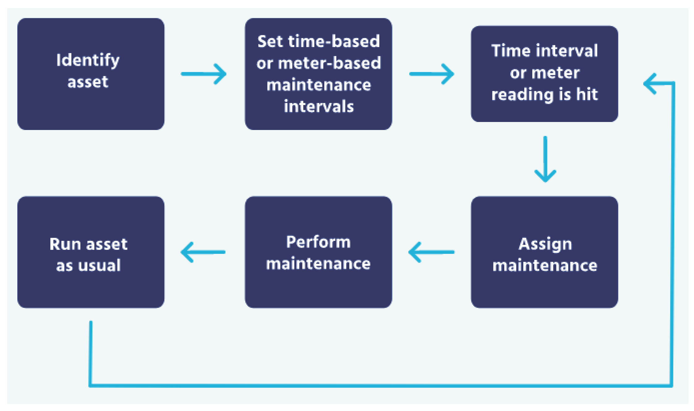
Figure 2.
A population (chromosomes) represents PMS.
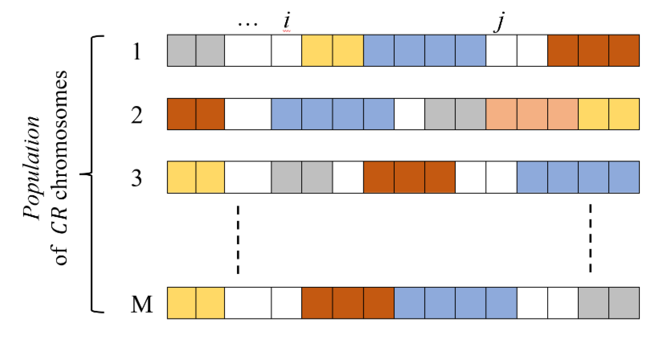
Figure 3.
Representation of chromosome, where number in gene represents equipment under maintenance.
Figure 3.
Representation of chromosome, where number in gene represents equipment under maintenance.

Figure 4.
Crossover operation.
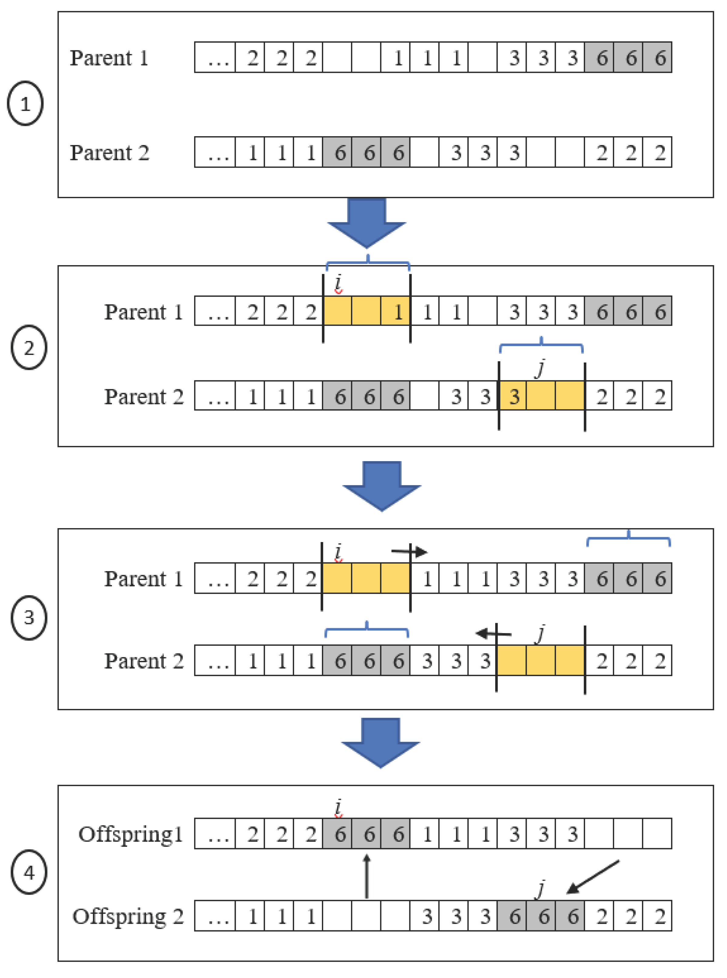
Figure 5.
Mutation operation.
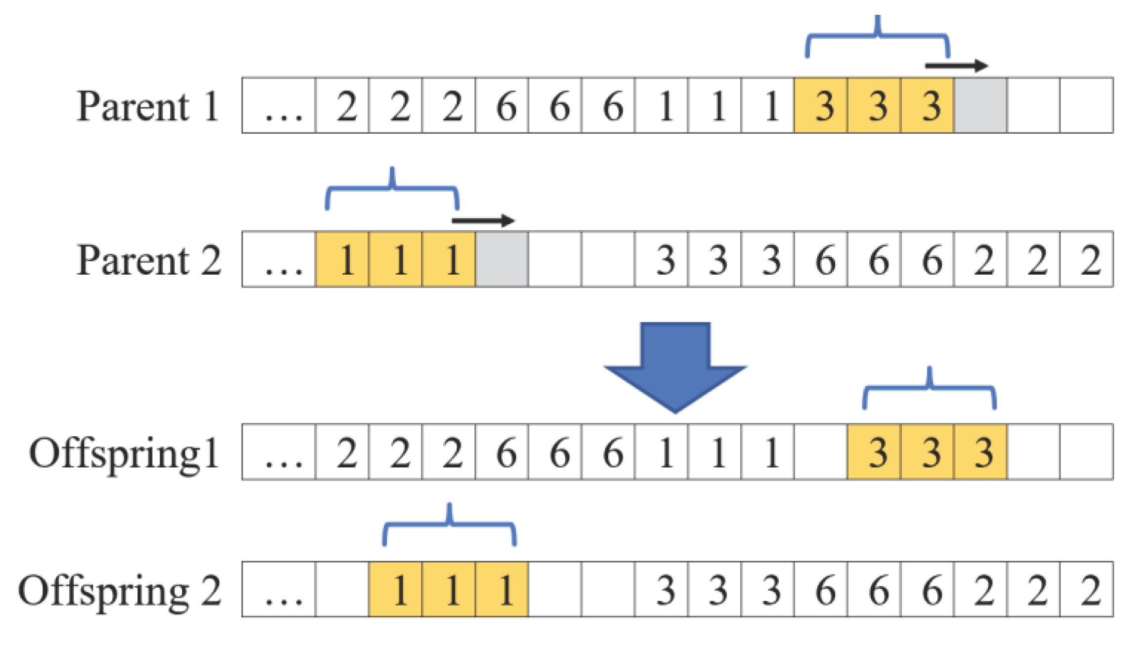
Figure 6.
PMS generation process for all equipment.
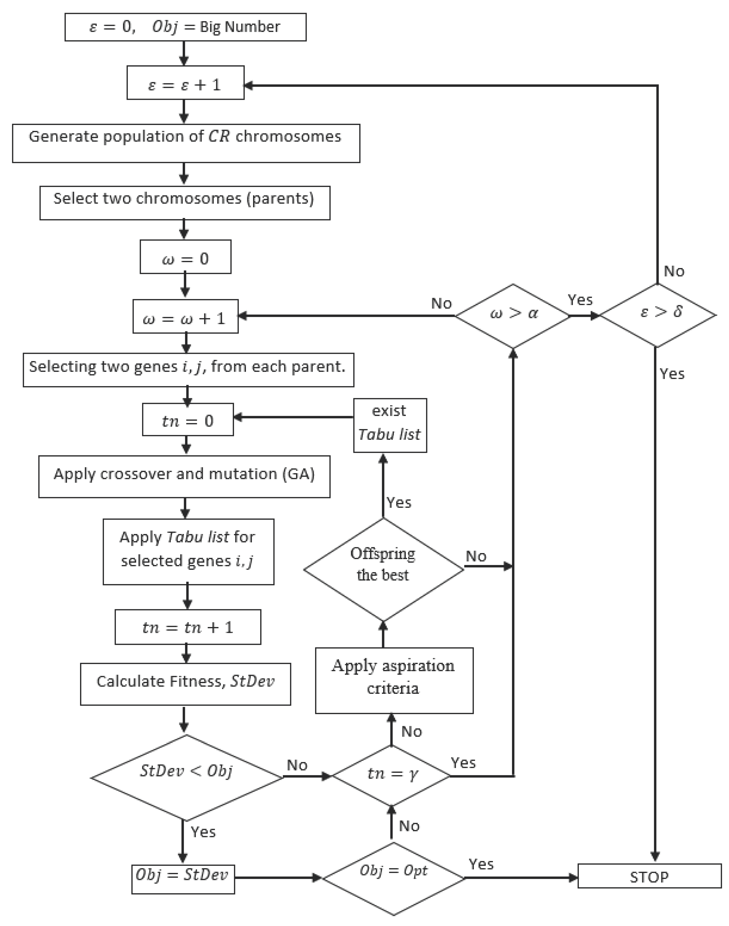
Figure 7.
a Total demand for water for 52 weeks. b Total demand for power for 52 weeks.
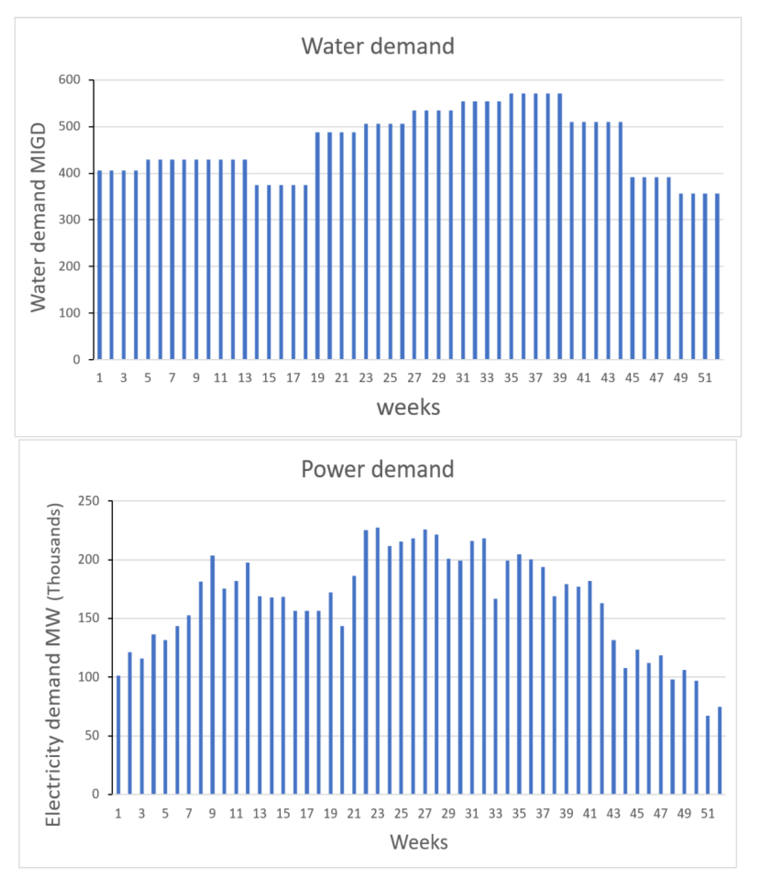
Figure 8.
a. Turbine equipment system output for Proposed method. b. Distiller equipment system output for Proposed method.
Figure 8.
a. Turbine equipment system output for Proposed method. b. Distiller equipment system output for Proposed method.
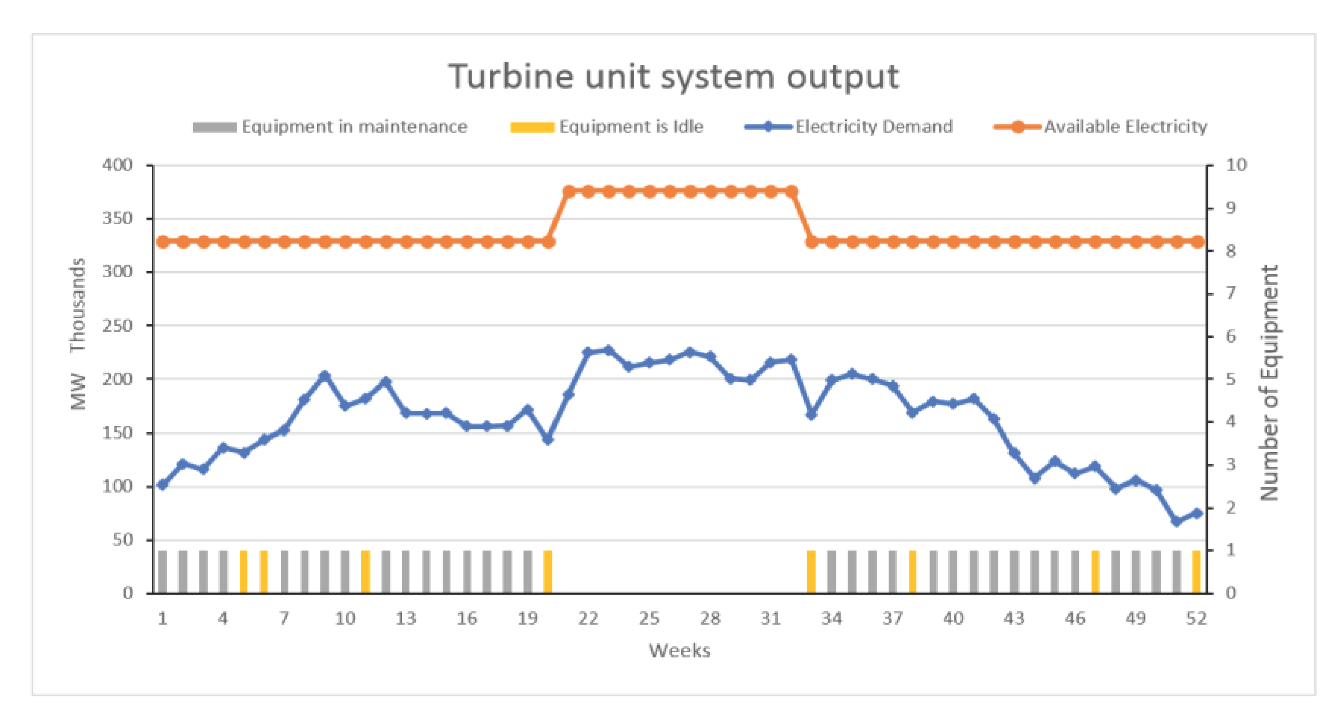
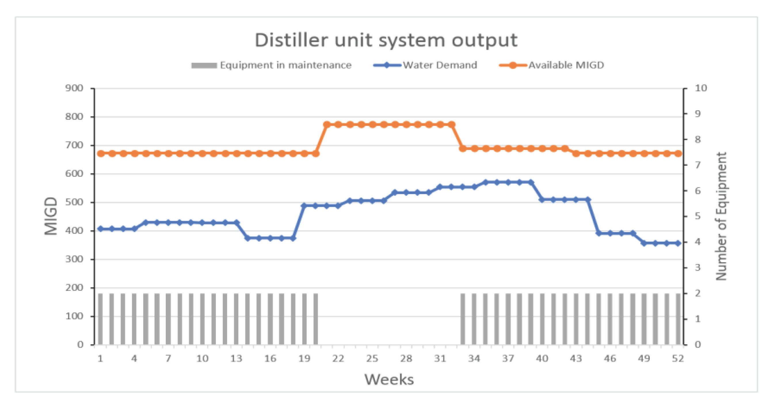
Figure 9.
a. Turbine equipment system output for MEW. b. Distiller equipment system output for MEW.
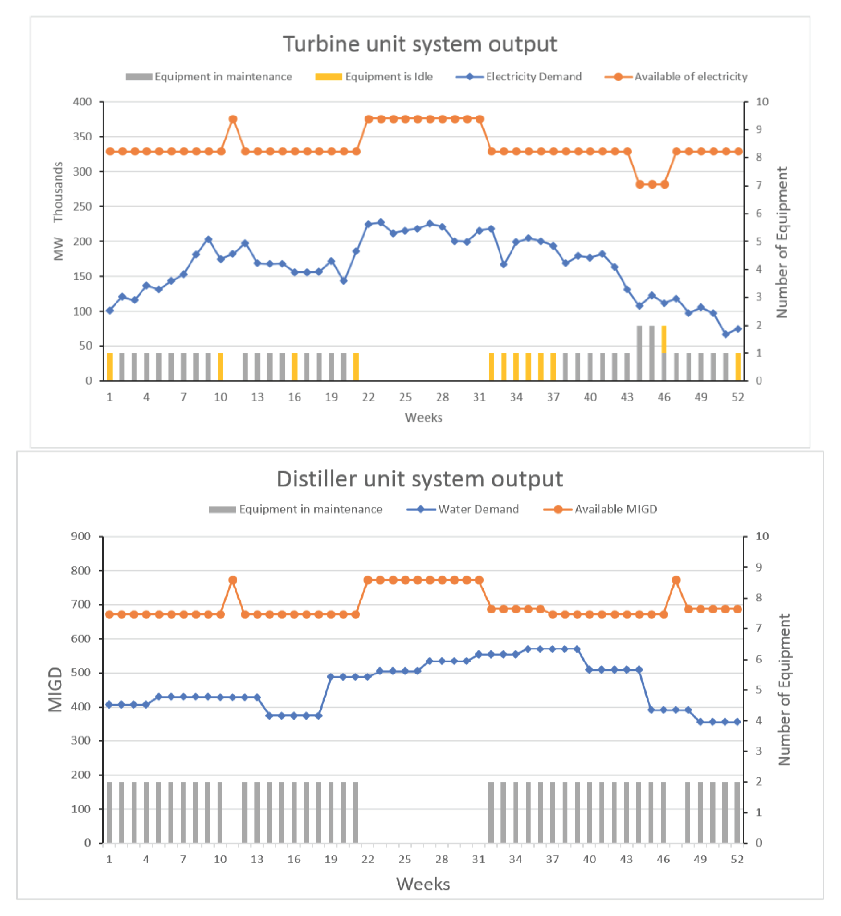
Figure 10.
a. Acomparison between the three methods in terms of CPU time (water surplus production). b. Acomparison between the three methods in terms of CPU time (electricity surplus production).
Figure 10.
a. Acomparison between the three methods in terms of CPU time (water surplus production). b. Acomparison between the three methods in terms of CPU time (electricity surplus production).
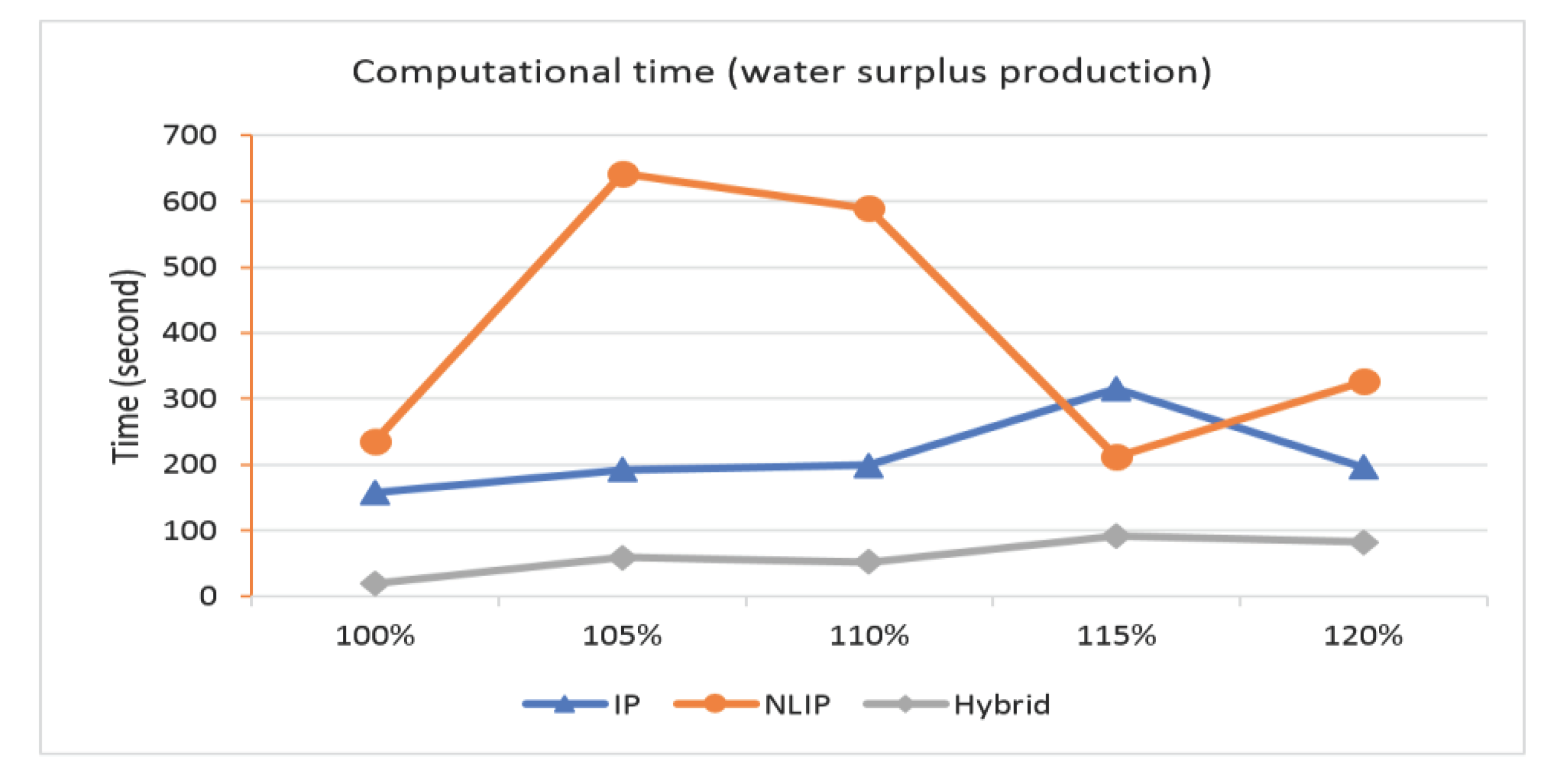
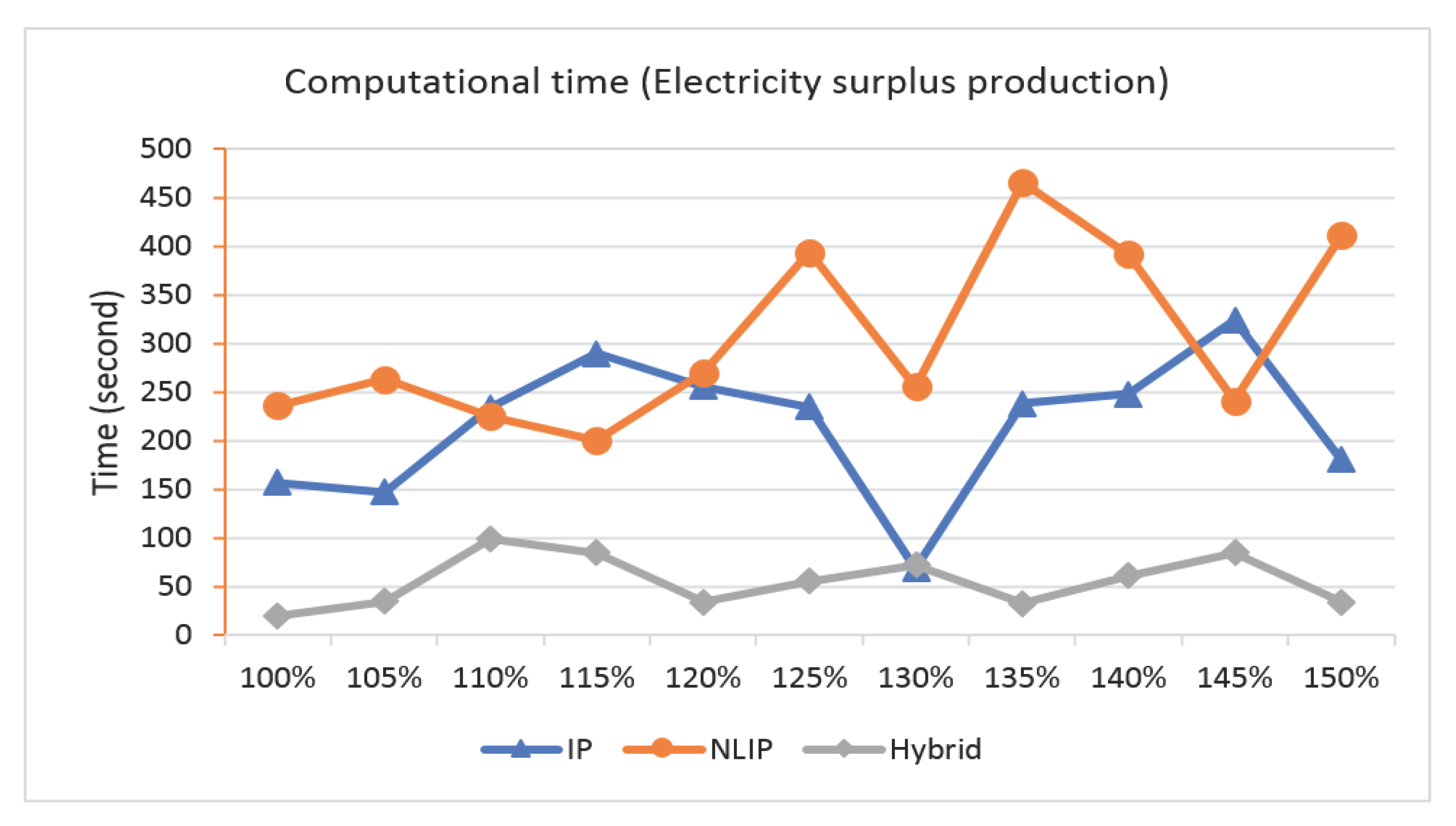

Table 1.
Production capacity for all equipment in Al-Zour station.
| Unit | Equipment | Production | Unit | Equipment | Production |
|---|---|---|---|---|---|
| 1 | D1 | 50.4 1 | 5 | D1 | 50.4 |
| D2 | 50.4 | D2 | 50.4 | ||
| R | 47,040 2 | R | 47,040 | ||
| 2 | D1 | 50.4 | 6 | D1 | 50.4 |
| D2 | 50.4 | D2 | 50.4 | ||
| R | 47,040 | R | 47,040 | ||
| 3 | D1 | 50.4 | 7 | D1 | 40.2 |
| D2 | 50.4 | D2 | 40.2 | ||
| R | 47,040 | R | 47,040 | ||
| 4 | D1 | 50.4 | 8 | D1 | 40.2 |
| D2 | 50.4 | D2 | 40.2 | ||
| R | 47,040 | R | 47,040 |
1 MIGD 2 MW.
| Symbol | CR | |||
| iteration | 10,000 | 50 | 4 | 100 |
| Proposal Approach | MEW | ||
| Distiller | St.Dev. | 59.6 | 70.724 |
| Average | 235.32 | 235.32 | |
| Min. Gap | 118.1 | 101.3 | |
| Turbine | St.Dev | 33519 | 33220.5 |
| Average | 175330 | 171712 | |
| Min. Gap | 124426 | 110971 |
Table 4.
PMS generated by the proposed model and by MEW.
| Week | Proposed Model | MEW | ||
|---|---|---|---|---|
| Equipment under PM | Idle | Equipment under PM | Idle | |
| 1 | B-2, D1-2, D2-2, R-2 | - | B-4, D1-4, D2-4 | R-4 |
| 2 | B-2, D1-2, D2-2, R-2 | - | B-4, D1-4, D2-4, R-4 | - |
| 3 | B-2, D1-2, D2-2, R-2 | - | B-4, D1-4, D2-4, R-4 | - |
| 4 | B-2, D1-2, D2-2, R-2 | - | B-4, D1-4, D2-4, R-4 | - |
| 5 | B-2, D1-2, D2-2 | R-2 | B-4, D1-4, D2-4, R-4 | - |
| 6 | B-5, D1-5, D2-5, R-5 | - | B-3, D1-3, D2-3, R-3 | - |
| 7 | B-5, D1-5, D2-5, R-5 | - | B-3, D1-3, D2-3, R-3 | - |
| 8 | B-5, D1-5, D2-5, R-5 | - | B-3, D1-3, D2-3, R-3 | - |
| 9 | B-5, D1-5, D2-5, R-5 | - | B-3, D1-3, D2-3, R-3 | - |
| 10 | B-5, D1-5, D2-5 | R-5 | B-3, D1-3, D2-3 | R-3 |
| 11 | B-3, D1-3, D2-3 | R-3 | - | - |
| 12 | B-3, D1-3, D2-3, R-3 | - | B-6, D1-6, D2-6, R-6 | - |
| 13 | B-3, D1-3, D2-3, R-3 | - | B-6, D1-6, D2-6, R-6 | - |
| 14 | B-3, D1-3, D2-3, R-3 | - | B-6, D1-6, D2-6, R-6 | - |
| 15 | B-3, D1-3, D2-3, R-3 | - | B-6, D1-6, D2-6, R-6 | - |
| 16 | B-6, D1-6, D2-6, R-6 | - | B-6, D1-6, D2-6 | R-6 |
| 17 | B-6, D1-6, D2-6, R-6 | - | B-5, D1-5, D2-5, R-5 | - |
| 18 | B-6, D1-6, D2-6, R-6 | - | B-5, D1-5, D2-5, R-5 | - |
| 19 | B-6, D1-6, D2-6, R-6 | - | B-5, D1-5, D2-5, R-5 | - |
| 20 | B-6, D1-6, D2-6 | R-6 | B-5, D1-5, D2-5, R-5 | - |
| 21 | - | - | B-5, D1-5, D2-5 | R-5 |
| 22 | - | - | - | - |
| 23 | - | - | - | - |
| 24 | - | - | - | - |
| 25 | - | - | - | - |
| 26 | - | - | - | - |
| 27 | - | - | - | - |
| 28 | - | - | - | - |
| 29 | - | - | - | - |
| 30 | - | - | - | - |
| 31 | - | - | - | - |
| 32 | - | - | B-7, D1-7, D2-7 | R-7 |
| 33 | B-7, D1-7, D2-7 | R-7 | B-7, D1-7, D2-7 | R-7 |
| 34 | B-7, D1-7, D2-7, R-7 | - | B-7, D1-7, D2-7 | R-7 |
| 35 | B-7, D1-7, D2-7, R-7 | - | B-7, D1-7, D2-7 | R-7 |
| 36 | B-7, D1-7, D2-7, R-7 | - | B-7, D1-7, D2-7 | R-7 |
| 37 | B-7, D1-7, D2-7, R-7 | - | B-2, D1-2, D2-2 | R-2 |
| 38 | B-8, D1-8, D2-8, R-8 | - | B-2, D1-2, D2-2, R-2 | - |
| 39 | B-8, D1-8, D2-8, R-8 | - | B-2, D1-2, D2-2, R-2 | - |
| 40 | B-8, D1-8, D2-8, R-8 | - | B-2, D1-2, D2-2, R-2 | - |
| 41 | B-8, D1-8, D2-8, R-8 | - | B-2, D1-2, D2-2, R-2 | - |
| 42 | B-8, D1-8, D2-8 | R-8 | B-1, D1-1, D2-1, R-1 | - |
| 43 | B-4, D1-4, D2-4, R-4 | - | B-1, D1-1, D2-1, R-1 | - |
| 44 | B-4, D1-4, D2-4, R-4 | - | B-1, D1-1, D2-1, R-1, R-7 | - |
| 45 | B-4, D1-4, D2-4, R-4 | - | B-1, D1-1, D2-1, R-1, R-7 | - |
| 46 | B-4, D1-4, D2-4, R-4 | - | B-1, D1-1, D2-1, R-7 | R-1 |
| 47 | B-4, D1-4, D2-4 | R-4 | R-7 | - |
| 48 | B-1, D1-1, D2-1, R-1 | - | B-8, D1-8, D2-8, R-8 | - |
| 49 | B-1, D1-1, D2-1, R-1 | - | B-8, D1-8, D2-8, R-8 | - |
| 50 | B-1, D1-1, D2-1, R-1 | - | B-8, D1-8, D2-8, R-8 | - |
| 51 | B-1, D1-1, D2-1, R-1 | - | B-8, D1-8, D2-8, R-8 | - |
| 52 | B-1, D1-1, D2-1 | R-1 | B-8, D1-8, D2-8 | R-8 |
Table 5.
a. Water Surplus production versus increased demand.b. Electricity Surplus production versus increased demand
Table 5.
a. Water Surplus production versus increased demand.b. Electricity Surplus production versus increased demand
| Water | Min. Gap | Time in second | ||||
| Increased Demand | Distiller | IP | NLIP | Hybrid | ||
| 100% | 100% | 118.1 | 157 | 236 | 20 | |
| 105% | 89.565 | 192 | 642 | 59 | ||
| 110% | 61.03 | 199 | 589 | 52 | ||
| 115% | 32.495 | 315 | 212 | 92 | ||
| 120% | 3.96 | 196 | 326 | 82 | ||
| Average | 211.8 | 401 | 61 | |||
| Electricity | Min. Gap | Time in second | ||||
| Increased Demand | Turbine | IP | NLIP | Hybrid | ||
| 100% | 100% | 124426 | 157 | 236 | 20 | |
| 105% | 114183 | 147 | 263 | 35 | ||
| 110% | 103941 | 234 | 225 | 99 | ||
| 115% | 93697.9 | 290 | 200 | 85 | ||
| 120% | 83455.2 | 256 | 270 | 34 | ||
| 125% | 73212.5 | 235 | 394 | 56 | ||
| 130% | 62969.8 | 69 | 256 | 72 | ||
| 135% | 52727.1 | 238 | 466 | 33 | ||
| 140% | 42484.4 | 248 | 392 | 61 | ||
| 145% | 32241.7 | 324 | 241 | 85 | ||
| 150% | 21999 | 181 | 411 | 34 | ||
| Average | 216.3 | 304.9 | 55.8 |
Disclaimer/Publisher’s Note: The statements, opinions and data contained in all publications are solely those of the individual author(s) and contributor(s) and not of MDPI and/or the editor(s). MDPI and/or the editor(s) disclaim responsibility for any injury to people or property resulting from any ideas, methods, instructions or products referred to in the content. |
© 2024 by the authors. Licensee MDPI, Basel, Switzerland. This article is an open access article distributed under the terms and conditions of the Creative Commons Attribution (CC BY) license (http://creativecommons.org/licenses/by/4.0/).
Copyright: This open access article is published under a Creative Commons CC BY 4.0 license, which permit the free download, distribution, and reuse, provided that the author and preprint are cited in any reuse.


