Ontological Reality of Time in Quantum Theory

1. Introduction

In quantum theory, unitary evolution is determined by the time parameter "t". But it is clear that the parameter t has no physical reality, since unitary evolution is deterministic. Indeed, it is a well-known fact that time is not physical in a deterministic world [3]. On the other hand, it is a matter of argument that there is a kind of "free will" in quantum mechanics [4,5,6,7]. Conway and Kochen gave a formal definition of free will [6,7]. According to their definition, the free will of particles, of quantum systems, can be defined. The outcome of a measurement on a quantum system is interpreted as the system’s response to that measurement. If the response of a localized quantum system (or local subsystem of a non-local quantum system) to a measurement is not a function of the information accessible to that (sub)system, then the (sub)system has free will. The free will determines the future by choosing what the next outcome will be and requires some notion of time. Obviously, free will is a consequence of what is called intrinsic probability [8,9,10] or absolute probability [11] in quantum mechanics. As stated by DeWitt quantum mechanical chance is not a measure of our ignorance [11]. However, if quantum mechanical probabilities are not a matter of our knowledge or ignorance, but are intrinsic to nature, then the "novelty" they bring provides important evidence that time is physical. The essence of our argument is that such intrinsic probabilities would indeed bring novelty that cannot be explained in epistemic ways. For example, consider a very long sequence of 0s (tails) and 1s (heads) generated by a quantum coin toss experiment. If such a sequence is long enough, it is a new sequence that has never been produced before in the history of the universe. Indeed, if we generate a second sequence of the same length, it will be a different sequence from the first.1 If quantum probabilities bring novelty, then time should not be an epistemic notion.

To prove the physical reality of time, we use the terminology of Harrigan and Spekkens [1]. We will do a reductio ad absurdum type proof and take as a presupposition that time is epistemic. Harrigan and Spekkens made their epistemic and ontic definitions for pure quantum states. Therefore, we need to treat time as a property of the quantum system. Indeed, one can prepare quantum states that intrinsically contain different possible histories and clock readings. Then, time can be interpreted as a property of such quantum states. A proof of the type of the Pusey-Barrett-Rudolph (PBR) theorem [2], applied to distinct quantum states in the sense that they encode different possible histories, different clock readings and consequently different times, proves that time is not epistemic. In fact, such a result is expected from the PBR theorem. Time comes from novelty and novelty is generated by intrinsic probabilities. The PBR theorem proves the physicality of the quantum state and thus implies that the state vector reduction is governed by a physical process. But quantum probabilities are related to this reduction and therefore cannot be epistemic in character. Hence, quantum probabilities are not the result of our ignorance but are indeed intrinsic to nature. Consequently, the time they produce cannot be epistemic either. Although in outline this argument is correct, it has some subtleties. Moreover, the following key question needs to be answered: To what extent is time, defined as the novelty generated by quantum probabilities, related to the notion of time we know from classical physics (e.g. general relativity)? Time is a very elusive concept to define. Defining time is as tricky as defining a number. Just as the number 2 is not 2 apples, 2 bananas or 2 objects, time is not the clock that measures it or the periodic dynamic system itself. But it can be defined with the help of an equivalence class of clocks. We define time as (a) the history that records make up, and (b) the proper time ticked by an ideal clock moving along a world line in spacetime, or equivalently the length of this world line in spacetime. However, neither of these two definitions is fundamental. The fundamental definition is (c) the novelty generated by a system; it is a sequence of new events or information. Here, novelty can be defined as the final state of the system not being a function of its previous state; the event or information generated does not depend on the previous state of the system. In order to provide a satisfactory proof in favour of the ontic character of time, all three definitions above should be shown to have a common intersection.

Idealist philosophy considers time as an illusion or an appearance of a special mode of perception [12]. In terms of the terminology we use in this paper, it is appropriate to classify time in idealist philosophy as epistemic. But if time is a kind of knowledge, where is this knowledge encoded? The information that represents time is the information of the observer, but since the observer is ultimately a quantum system, time information should be encoded into observer’s wave function. The observer is in a "knowledge state" that encodes time information. However, there is a subtle point to note here. The wave function we will apply the PBR proof to is not the wave function of the observer. Whether time has an ontic or epistemic essence, the observer can always be in a state that encodes the information of time. It is analogous to the fact that although energy is an ontic notion, the observer who knows a particular value of energy is in a state that encodes this information. Our reasoning is not about time information states of the observer, but about the question of whether a quantum state containing time as an intrinsic property is relative to the observer’s knowledge. We will use the term time state for a state that includes time as an intrinsic property. If time is encoded on $|\psi >$ as a unitary evolution parameter, it is pure information and does not correspond to physical reality. Indeed, multiplying the distinct states $|{\psi }_0>$ and $|{\psi }_1>$ in the proof of the PBR theorem (eqn.2 of ref. [2]) by the unitary evolution operator does not affect the proof. In the PBR proof, the time parameter for unitary evolution is not relevant. The time that can be related to physical reality is not related to unitary evolution, but must originate in free will. The state encoding time, which is a potential candidate to be physical, is expected to be a state involving quantum superpositions of different histories and different clock readings. The different possible histories determined by different records are encoded as an intrinsic property of such a state.

In fact, the PBR theorem has largely proved that time is not epistemic. It remains to take a small step further. The quantum states proved to be ontic in the theorem involve superpositions of qubits. These superpositions can be interpreted as time states, since distinct superpositions bring different novelties and in this sense include time as an intrinsic property. However, the PBR theorem was constructed to prove that $\psi$ is ontic, not to show that time is ontic. It is not an obvious fact that time is ontic in a $\psi$-ontic ontological model.2 In our PBR-type proof, we provide a stronger proof in favor of the ontic character of time by showing that the novelty of quantum probabilities can be related to the proper time measured by a clock moving along a world line in spacetime within the framework of general relativity. Thus we show that definitions (a), (b) and (c) of time have a common intersection. In Section 2 we will discuss how to prepare a time state compatible with the notion of Newtonian time and perform a PBR-type proof. There, the concept of time will be treated as a notion produced by free will in the sense that it makes different histories possible. In Section 3 we will make a similar proof to show that a time state compatible with the notion of time in general relativity is ontic. As we will demonstrate, the free will is also capable of generating the notion of time as measured by a dynamic clock moving along a world line. In Section 4 the details of the proof will be given and we will discuss what we have actually proved. We will show that there are two distinct lines of reasoning about the ontic character of time.

Finally, there are a few important points we would like to emphasize. First, our proof requires, along with the presuppositions of the PBR theorem, a presupposition we call the universality of quantum probabilities. The assumption of universality of quantum probabilities states that the nature of the probabilities is independent from the real physical state of the preparation and the physical system used in the measurement procedure, but depends only on the quantum superposition that has been prepared, i.e. the nature of probabilities is determined only by the pure quantum state or the ontic state corresponding one-to-one to that quantum state. By the term "nature" we refer to the origin of probabilities, not their numerical values. Quantum theory predicts that the numerical values of probabilities do not depend on the preparation procedure used, but only on the quantum state that has been prepared, i.e. the numerical values of probabilities are the same for all different preparations of the same quantum state. In our proof in this paper, we assume the correctness of the predictions of quantum theory. However, quantum formalism is silent about the nature of probabilities. Our universality assumption states that the only element that determines the nature of probabilities, i.e. their intrinsic or statistical character (ontic or epistemic origin), is the pure quantum state being prepared. Note that our assumption is a statement about pure quantum states only. Under this assumption, when it comes to the novelty generated by probabilities, it is irrelevant whether these probabilities are associated with a spin measurement or a nuclear decay process or etc.. Second, our proof does not prove the existence of a universal notion of time. It is known that the universe as a whole is constrained by the Wheeler-DeWitt equation and does not evolve [13]. On the other hand, it is possible to study a subsystem of the universe as an ideal clock for the remaining subsystems [14]. Thus, through this mechanism, unitary evolution can be recovered. However, the result does not change; unitary evolution is deterministic and an ontic notion of time cannot be defined. The notion of time, the physical reality of which we argue for, arises from the novelty of intrinsic probabilities (free will). Such a notion of time, in relation to the reduction of the state vector, should not be a property of the system as a whole, but of its subsystems. Indeed, the reduction takes place with respect to a subsystem defined as an observer. This gives us a notion of time that is not globally defined but locally applicable. We would like to point out that whether reduction occurs spontaneously or whether the observer has a direct role in it is beside the point. What is important here is that even if the observer has a role in the reduction, it is not a role that can only be defined in an epistemic way.

2. History Superpositions and Time State

Let us imagine an experimental setup that resembles the Schrödinger’s cat gedankenexperiment. There is a closed box that we cannot see inside. Inside the box, instead of a cat, there is a demon conducting quantum coin toss experiments. If the result is tail, demon prepares a qubit state of $|0>$ and if it is head, it prepares a qubit state of $|1>$ and attaches it on a long tape. The demon conducts successive experiments and attaches the resulting quantum states to the tape one after the other. Therefore, the order of the attached state on the tape indicates the time order of the experiment to which it belongs. We should note, however, that since we do not assume from the outset an ontic notion of time that determines the order of experimental outcomes, history is simply a sequence of heads and tails events. Accordingly, different orders of qubits $|0>$s and $|1>$s on the tape represent different histories. It should also be noted that the demon can perform the quantum coin toss experiment with different experimental setup parameters and determine the probabilities of tail and head outcomes. So the quantum coin toss experiment we are considering here does not have to be an experiment with 50%-50% equal probability. The demon could also write the results of the experiments on the tape in the classic 0 and 1 bits. But instead he writes them as qubits. The idea is to encode the information into a quantum system. Suppose the demon performs N consecutive experiments and writes down the results (as qubits) on a tape. In this case, the tape is a quantum system that encodes both the results of the experiments and the order in which these results were obtained. Specifically, the tape defines a record state, denote it by $|\mathrm{Rec}.;\mathrm{N}>$. According to the demon, the state $|\mathrm{Rec}.;\mathrm{N}>$ represents a history. But to an observer outside the box, it represents $2^N$ possible histories. Denote the probabilities of the outcomes of the jth quantum coin toss experiment performed by the demon by $p_0^{\left(j\right)}$ (probability of getting tail) and $p_1^{\left(j\right)}$ (probability of getting head). Accordingly, the observer writes down the following record state:

$$\begin{array}{c}\hfill |\mathrm{Rec}.;\mathrm{N}{>}_0=|{\psi }_0^{\left(1\right)}>\otimes |{\psi }_0^{\left(2\right)}>\otimes ...\otimes |{\psi }_0^{\left(N\right)}>\end{array}$$

(2.1)

$$\begin{array}{c}\hfill |{\psi }_0^{\left(j\right)}>=\sqrt{p_0^{\left(j\right)}}|0>+\sqrt{p_1^{\left(j\right)}}|1>;1\le j\le N\end{array}$$

(2.2)

Here, the complex phases in the coefficients of the $|0>$ and $|1>$ states are neglected and the coefficients are taken real. This can be done because complex phases can be removed by a unitary transformation without disturbing the normalization. The subscript 0 below the $|\mathrm{Rec}.;\mathrm{N}{>}_0$ and $|{\psi }_0^{\left(j\right)}>$ states indicates a particular state prepared through the device parameters of each experiment. We assume that the device parameters and the associated probabilities of each experiment are known both by the demon and by the observer. Now consider a second record state, distinct from the first one, prepared using different device parameters (the probabilities are different for at least one j). Let us denote this state, which is distinct from the first one, by the subscript 1.

$$\begin{array}{c}\hfill |\mathrm{Rec}.;\mathrm{N}{>}_1=|{\psi }_1^{\left(1\right)}>\otimes |{\psi }_1^{\left(2\right)}>\otimes ...\otimes |{\psi }_1^{\left(N\right)}>\end{array}$$

(2.3)

$$\begin{array}{c}\hfill |{\psi }_1^{\left(j\right)}>=\sqrt{p_0^{\prime \left(j\right)}}|0>+\sqrt{p_1^{\prime \left(j\right)}}|1>;1\le j\le N\end{array}$$

(2.4)

History is made up of records. (2.1) and (2.3) are two distinct states, containing different possible histories as an intrinsic property. These states are examples of the time states we defined in the introduction section. Recall that, by this term we mean a quantum state in which time information is encoded as an intrinsic property. Indeed, the possible histories, and hence the time defined by those histories, are encoded in the states (2.1) and (2.3) as superposition, which is a fundamental property of quantum states. There are many possible histories before the observer reads the qubits on the tape. When the observer reads the tape, a single history emerges. We would like to emphasize that (2.1) and (2.3) are two distinct states, only in the sense that they encode different possible histories. According to the terminology of Ref. [1], if time is epistemic, then a change in time does not lead to a change in observable reality. The states given by (2.1) and (2.3) introduce different novelties in that they encode different possible histories. As we will show, a change in time, which corresponds to a change from (2.1) to (2.3), implies a change in observable reality.

Some readers may object and say that when the observer reads the tape, she does not see different histories for different orders of outcome events of quantum coin toss experiments, but she sees a list of different outcomes for the same history. This objection is due to the confusion between the notion of time, which we will prove to be physical, and the notion of time, which we can call "prior or pre time" used in the ordering of experimental outcomes. In order to avoid some confusion, we would also like to remind the following point: The time that we will prove to be physical is the time that arises from the novelty of intrinsic probabilities; it is not the time that is the internal sense of the human being. In ordering the results of the experiments, the demon uses a notion of time, i.e. a prior or pre notion of time is assumed. This prior notion of time could be based on the demon’s internal sense or perhaps based on a dynamical system he uses as a clock. However, we cannot assume that this prior notion of time is ontic, because then we would be presupposing what we are going to prove. Quantum probabilities generate a “new” sequence of heads and tails that we assume constitutes time. It is this notion of time that we will prove to be ontic. In this sequence generated by intrinsic quantum probabilities, a change in the order of heads and tails corresponds to a change in history. The states $|\mathrm{Rec}.;\mathrm{N}{>}_0$ and $|\mathrm{Rec}.;\mathrm{N}{>}_1$ encode different novelties brought about by intrinsic probabilities. In this sense, these states fulfill our definition of "time states".

(2.1) and (2.3) are two distinct states just because they encode different times. But if time is an epistemic notion, then there exist at least two probability distributions (epistemic states in the terminology of [1]) ${\mu }_0\left(\lambda \right)$ and ${\mu }_1\left(\lambda \right)$ such that ${\mu }_0\left(\lambda \right)\bigcap {\mu }_1\left(\lambda \right)\ne \varnothing$ [1,2]. In other words, there exist at least two states $|\mathrm{Rec}.;\mathrm{N}{>}_0$ and $|\mathrm{Rec}.;\mathrm{N}{>}_1$ such that the ontic state ($\lambda$) is compatible with both. Let us note that here we implicitly use the assumption of universality of quantum probabilities. The demon can use different experimental setups to prepare the superposition. For example, he could use a spin measurement experiment or he could use radioactive decay. In the end, the novelty brought by intrinsic probabilities is of the very same nature, regardless of how the demon prepares the quantum superposition. This assumption may seem redundant because quantum theory makes the same predictions for the same quantum superposition, albeit prepared in different ways. However, if the quantum theory is $\psi$-incomplete, then it is worth considering the possibility that the time information may be encoded on the supplementary variable, not on $\psi$. In such a case, in two different preparations of the same quantum state by the demon, the encoded time information may be different. Then, the quantum states $|\mathrm{Rec}.;\mathrm{N}{>}_0$ and $|\mathrm{Rec}.;\mathrm{N}{>}_1$ do not represent all the physical states encoding time. The assumption of the universality of quantum probabilities saves us from such a dilemma. Under this assumption, different preparations giving the same quantum superposition do not encode different times.

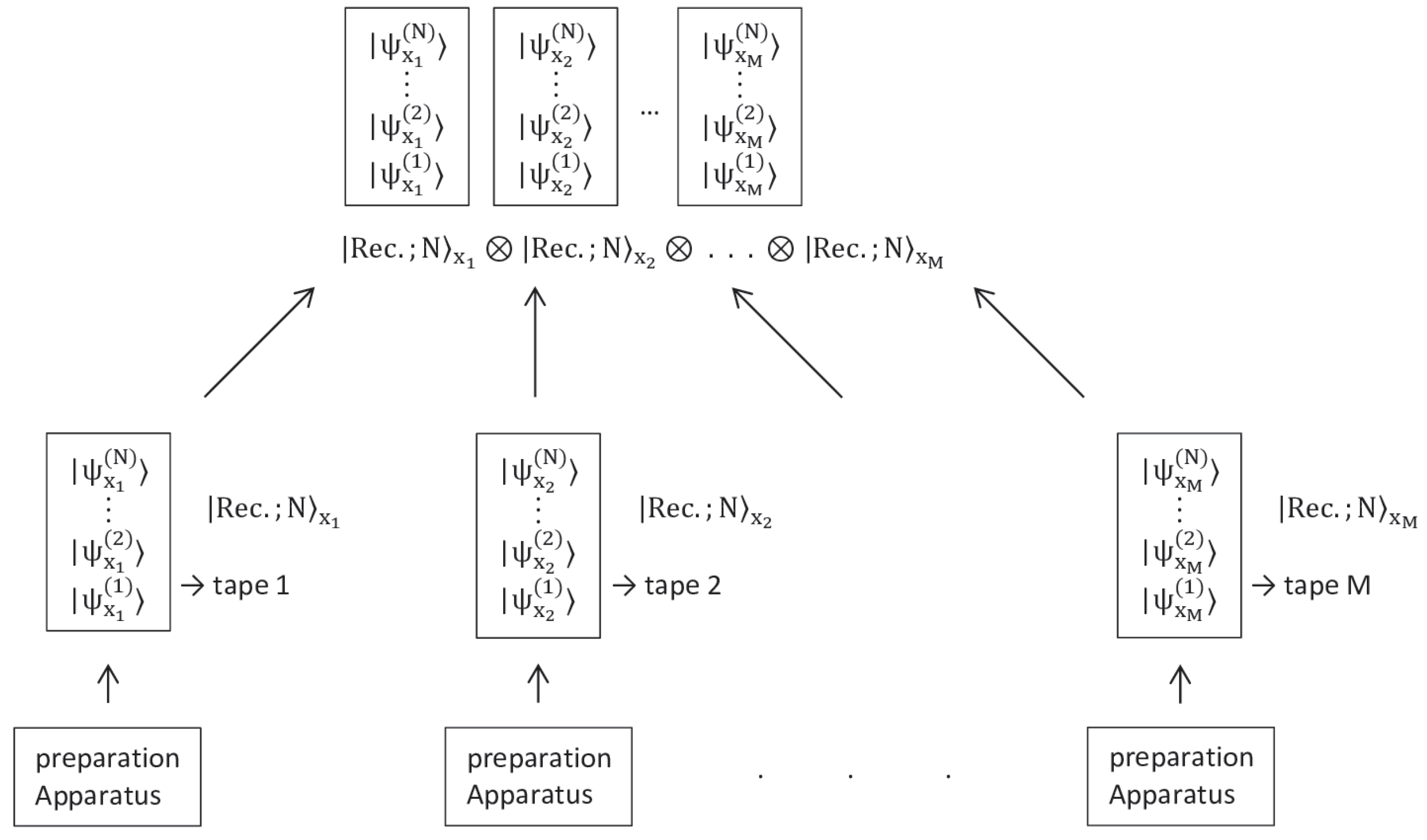
Suppose we have M independent record state preparations, i.e. M long tapes, each containing N qubits. These prepared systems are brought together for measurement (see Figure 1). Depending on which of the two preparations is employed each time, M systems are prepared in one of the following quantum states:

$$\begin{array}{c}\hfill |\mathrm{Rec}.;\mathrm{N};x_1,...,x_M>=|\mathrm{Rec}.;\mathrm{N}{>}_{x_1}\otimes |\mathrm{Rec}.;\mathrm{N}{>}_{x_2}\otimes ...\otimes |\mathrm{Rec}.;\mathrm{N}{>}_{x_M}\end{array}$$

(2.5)

where, $x_m\in \{0,1\};1\le m\le M$. The qubits in the same jth row of each of the M tapes brought together are of the form

$$\begin{array}{c}\hfill |{\psi }_{x_1}^{\left(j\right)}>\otimes |{\psi }_{x_2}^{\left(j\right)}>\otimes ...\otimes |{\psi }_{x_M}^{\left(j\right)}>.\end{array}$$

(2.6)

For a given j, $2^M$ different such quantum states can be constructed. If time is epistemic, then there exist at least two quantum states $|{\psi }_0^{\left(j\right)}>$ and $|{\psi }_1^{\left(j\right)}>$ such that ${\mu }_{{\psi }_0^{\left(j\right)}}\left(\lambda \right)\bigcap {\mu }_{{\psi }_1^{\left(j\right)}}\left(\lambda \right)\ne \varnothing$. Accordingly, with a non-zero probability q, ontic state $\lambda$ lies in the intersection. Since the preparations are independent, the complete physical state of the systems prepared by the demons is compatible with any of these $2^M$ quantum states with probability at least $q^M$. However, it can be shown that there is a joint measurement on this M system such that each outcome has probability zero on at least one of the states of (2.6). This leads to a contradiction! Although our reasoning here considers the measurement on a fixed jth row of the tape, j is arbitrary and a similar conclusion can be drawn for each j. To show the existence of such a joint measurement, let us define the following unitary operator

$$\begin{array}{c}\hfill L_{{\overline{\alpha }}^{\left(j\right)}}=cos{\overline{\alpha }}^{\left(j\right)}|0><0|+sin{\overline{\alpha }}^{\left(j\right)}|0><1|-sin{\overline{\alpha }}^{\left(j\right)}|1><0|+cos{\overline{\alpha }}^{\left(j\right)}|1><1|\end{array}$$

(2.7)

where, ${\overline{\alpha }}^{\left(j\right)}={\displaystyle \frac{{\alpha }_0^{\left(j\right)}+{\alpha }_1^{\left(j\right)}}{2}}$, ${\alpha }_0^{\left(j\right)}=arccos\left(\sqrt{p_0^{\left(j\right)}}\right)$ and ${\alpha }_1^{\left(j\right)}=arccos\left(\sqrt{p_0^{\prime \left(j\right)}}\right)$. The effect of $L_{{\overline{\alpha }}^{\left(j\right)}}$ on (2.2) and (2.4) transforms them into the form

$$\begin{array}{c}\hfill L_{{\overline{\alpha }}^{\left(j\right)}}|{\psi }_x^{\left(j\right)}>=cos\left({\displaystyle \frac{\Delta {\alpha }^{\left(j\right)}}{2}}\right)|0>+{(-1)}^{x}sin\left({\displaystyle \frac{\Delta {\alpha }^{\left(j\right)}}{2}}\right)|1>\end{array}$$

(2.8)

which coincides with Equation (2.2) in ref. [2]. Here, $\Delta {\alpha }^{\left(j\right)}={\alpha }_0^{\left(j\right)}-{\alpha }_1^{\left(j\right)}$ and $x\in \{0,1\}$. Therefore, the measurement used in the proof of the PBR theorem can be applied hereafter. Indeed, the following joint measurement fulfills the required condition; each outcome has probability zero on at least one of the states of (2.6):

$$\begin{array}{c}\hfill <x_1,x_2,...,x_M|U_{PBR}{L}_{{\overline{\alpha }}^{\left(j\right)}}^{\otimes M}|{\psi }_{x_1}^{\left(j\right)},{\psi }_{x_2}^{\left(j\right)},...,{\psi }_{x_M}^{\left(j\right)}>=0\end{array}$$

(2.9)

For the definition of operator $U_{PBR}$, see Appendix B equation (0.62). Here M is chosen to be large enough so that $2^{1/M}-1\le tan\left({\displaystyle \frac{\Delta {\alpha }^{\left(j\right)}}{2}}\right)$.

There are some subtle points in the above proof that time is not epistemic. First, we applied the PBR-type proof separately to each row of the long tape described by $|\mathrm{Rec}.;\mathrm{N}>$. By this we actually prove the physicality of time represented by 1 qubit of information. The long tape of N qubits could represent a long history. But there is no need to show that such a long time interval is ontic. Indeed, the novelty introduced by quantum probabilities is discrete and novelties, each represented by 1 qubit of information, combine to form a long time interval. The assumption of universality of quantum probabilities implies that each small 1 qubit chunk of time has the same nature as the next. Similarly, instead of a two-level quantum system, the demon could have introduced the novelties with a three- or multi-level quantum system. Again, nothing changes due to our universality assumption; only 2-level quantum systems can be considered without loss of generality. The second point we should emphasize is as follows. The observer and the demon are non-relativistic agents. If physical time, i.e. the novelty brought by quantum probabilities, is to be correlated with a ticking clock, such a clock would be a clock that measures Newtonian time. Accordingly, the physical time generated by quantum probabilities can to some extent be harmonized with a Newtonian notion of time, albeit in a restricted sense. For example, we can order the sequence of events resulting from successive quantum state reduction processes according to Newtonian time and put some kind of (Newtonian) time order between events. However, the notion of time in the theory of relativity is quite different. The question then arises: can some kind of relationship be established between the physical time introduced by quantum probabilities and the notion of time in relativity theory? In Section 3 we will show that the answer to this question is positive.

3. Time State Representing the Superposition of Proper Times

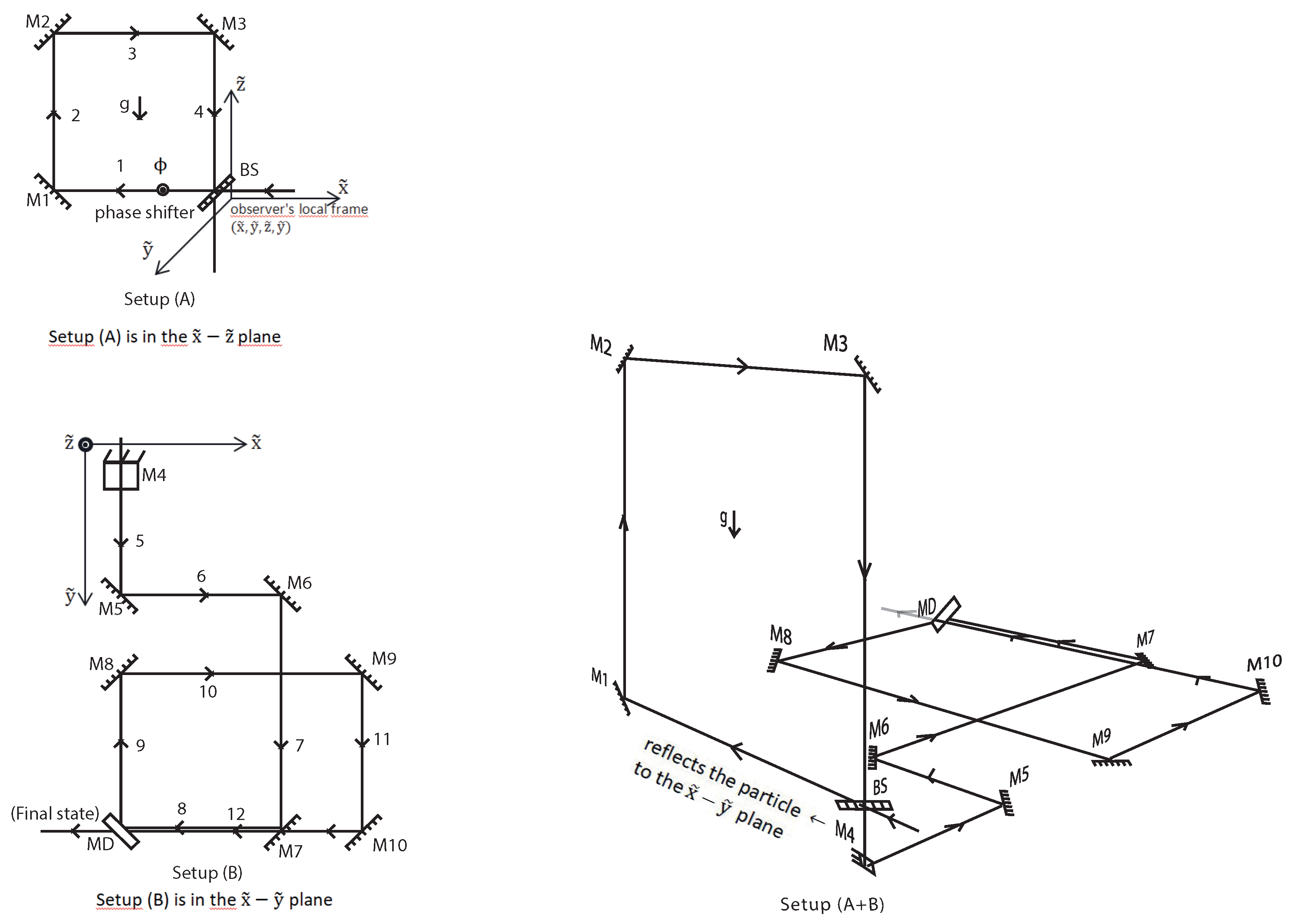
Consider the experimental setup located on the Earth’s surface, shown in Figure 2. The setup is small enough that the gravitational field is assumed to be uniform throughout the setup. Part (A) of the setup is located vertically and the arms at different heights are subjected to different gravitational potentials. On the other hand, part (B) is located horizontally and the arms are at the same gravitational potential. A particle enters the setup through a beam splitter (BS) with adjustable transmission/reflection probabilities. The particle has an evolving internal degree of freedom that can be defined as a "clock". The behavior of a particle with such a clock internal degree of freedom moving in interferometers has been studied previously [15,16]. The setups are in a closed box that the observer cannot see inside. In one corner of the setup (B), there is an apparatus called a mirrored door (MD). The MD acts like a mirror until the observer presses a button. But once the button is pressed, the mirror opens and allows the particle to exit. After waiting long enough, the observer opens the MD by pressing a button and lets the particle out. We assume that the time of flight of the particle on each arm in setup (A) is equal and given by T with respect to the observer’s time. The total flight times along paths 1-2-3-4, 5-6-7-8 and 9-10-11-12 are equal and given by $4T$. We define the total motion of the particle in one of these piecewise paths (1-2-3-4, 5-6-7-8 or 9-10-11-12 ) as one revolution. Hence, it takes $4T$ time for the particle to make one revolution in (A) or (B). The observer presses the button after waiting for a period of $4TN$, where $N\in {\mathbb{Z}}^{+}$. The total number of revolutions of the particle in the setup (A) or (B) is determined by the transmission/reflection probabilities of the BS. However, the setup (A) and (B) are at different gravitational potentials. Therefore, how much time the particle spends in which setup (the number of revolutions in setup (A) or (B)) causes the particle’s internal clock to be affected differently by gravitational time dilation. Indeed, the internal clock runs slightly faster in setup (A) than in setup (B). Consequently, when the observer presses the button and opens the MD, she encounters a particle state in superposition of different proper times.

Let us now carry out a quantitative analysis to understand the behavior of the quantum mechanical clock in the gravitational field. The spacetime on the Earth’s surface can be described by the Schwarzschild metric in isotropic form [17].

$$\begin{array}{c}\hfill d{s}^2={\displaystyle \frac{{(1-MG/2c^{2}z)}^2}{{(1+MG/2c^{2}z)}^2}}{c}^{2}d{t}^2-{\left(1+{\displaystyle \frac{MG}{2c^{2}z}}\right)}^4\left(d{z}^2+z^2(d{\theta }^2+{sin}^2\theta d{\varphi }^2)\right)\end{array}$$

(3.10)

Here the isotropic coordinate z is related to the radius coordinate of the Schwarzschild metric in standard form as $z=[r-MG/c^2+\sqrt{r^2-2MGr/c^2}]/2$. On the surface of the Earth, it is a good approximation to take $z\simeq r$; the difference is of the order of ${10}^{-9}$. Define the (Newtonian) gravitational potential as $\varphi \left(z\right)=-MG/z$. If the metric (3.10) is expanded to the series and the terms up to order of $\varphi {\left(z\right)}^2/c^4$ are taken into account, we obtain

$$\begin{array}{c}\hfill {\left({\displaystyle \frac{d\tau }{dt}}\right)}^2\simeq (1+{\displaystyle \frac{2\varphi \left(z\right)}{c^2}}+{\displaystyle \frac{2\varphi {\left(z\right)}^2}{c^4}})-{\displaystyle \frac{1}{c^2}}(1-{\displaystyle \frac{2\varphi \left(z\right)}{c^2}})v_I^2\end{array}$$

(3.11)

where $v_I=\sqrt{{\left({\displaystyle \frac{dz}{dt}}\right)}^2+z^2{\left({\displaystyle \frac{d\theta }{dt}}\right)}^2+z^2{sin}^2\theta {\left({\displaystyle \frac{d\varphi }{dt}}\right)}^2}$ is the velocity with respect to the isotropic coordinates and $\tau$ is the proper time, i.e. $d{\tau }^2={\displaystyle \frac{d{s}^2}{c^2}}$. However, this velocity is not defined in terms of the local coordinates of the observer on the Earth’s surface. The observer is located on the earth’s surface with its origin on the BS of the setup (see Figure 2). Since the spatial scale of the setup is sufficiently small, it is a good approximation to assert that the velocity of the particle moving through the setup is defined by the local coordinates of the observer. Then, the following relation applies for the magnitude of the local velocity $v\simeq (1-{\displaystyle \frac{2\varphi \left(R\right)}{c^2}})v_I$, where R is the radius of the earth. Similarly, the observer writes the Schrödinger equation in her local coordinates ($\tilde{t},\tilde{x},\tilde{y},\tilde{z}$) for the metric $d{s}^2=c^{2}d{\tilde{t}}^2-d{\tilde{z}}^2-d{\tilde{x}}^2-d{\tilde{y}}^2$ and describes the quantum mechanical evolution of the particle with this equation. Under this approximation, general relativistic contributions are analyzed in terms of correction terms to the Hamiltonian [15]. In the rest frame of the particle, the evolution of the clock is described by the equation $i\hslash {\displaystyle \frac{\partial \psi }{\partial \tau }}=H_{clock}\psi$. However, since the time coordinate of the observer is $\tilde{t}$, the evolution of the clock relative to the observer is described by the equation

$$\begin{array}{c}\hfill i\hslash {\displaystyle \frac{\partial \psi }{\partial \tilde{t}}}={\tilde{H}}_{clock}\psi \end{array}$$

(3.12)

where,

$$\begin{array}{c}\hfill {\tilde{H}}_{clock}=\left({\displaystyle \frac{d\tau }{d\tilde{t}}}\right)H_{clock}\end{array}$$

(3.13)

$$\begin{array}{c}\hfill \left({\displaystyle \frac{d\tau }{d\tilde{t}}}\right)\simeq {\left[{\displaystyle \frac{1+\frac{2\varphi \left(z\right)}{c^2}+\frac{2\varphi {\left(z\right)}^2}{c^4}}{1+\frac{2\varphi \left(R\right)}{c^2}}}-\left({\displaystyle \frac{1-\frac{2\varphi \left(z\right)}{c^2}}{1-\frac{2\varphi \left(R\right)}{c^2}}}\right){\displaystyle \frac{v^2}{c^2}}\right]}^{1/2}.\end{array}$$

(3.14)

Here we made use of equation (3.11) and the definition of local velocity. Note that for $v=0$, expression (3.14) gives the gravitational redshift factor between the rest frame of the particle and the local frame of the observer. If the Hamiltonian is expanded into a series and the terms of order ${\displaystyle \frac{{\varphi }^2}{c^4}},{\displaystyle \frac{v^4}{c^4}},{\displaystyle \frac{\varphi v^2}{c^4}}$ and higher are neglected, we get

$$\begin{array}{c}\hfill {\tilde{H}}_{clock}\simeq {\left(1+{\displaystyle \frac{2\varphi \left(R\right)}{c^2}}\right)}^{-1/2}\left(1+{\displaystyle \frac{\varphi \left(z\right)}{c^2}}-{\displaystyle \frac{v^2}{2c^2}}\right)H_{clock}.\end{array}$$

(3.15)

The multiplier ${\left(1+{\displaystyle \frac{2\varphi \left(R\right)}{c^2}}\right)}^{-1/2}$ is the gravitational redshift factor between the Minkowski observer at infinity and the local observer at $z\simeq R$. Therefore, it is possible to interpret the term other than the redshift factor as the Hamiltonian with respect to the Minkowski observer at infinity. As the rest frame clock Hamiltonian, we use the two-level Hamiltonian

$$\begin{array}{c}\hfill H_{clock}=E_0|0><0|+E_1|1><1|\end{array}$$

(3.16)

used in ref. [15]. Then, in the rest frame of the particle, the clock state ($|\tau >$) evolves as

$$\begin{array}{ccc}\hfill |\tau >=& & e^{{\displaystyle \frac{-i}{\hslash }}{H}_{clock}\tau }|{\tau }_0>\hfill \\ \hfill =& & {\displaystyle \frac{e^{-i{E}_0\tau /\hslash }}{\sqrt{2}}}\left(|0>+e^{-i\Delta E\tau /\hslash }|1>\right)\hfill \end{array}$$

(3.17)

, while for a clock moving on the surface of the earth the clock state evolves (according to the Minkowski observer at infinity) as

$$\begin{array}{ccc}\hfill |\tau >=& & e^{{\displaystyle \frac{-i}{\hslash }}{\int }_{path}dt\left(1+{\displaystyle \frac{\varphi \left(R\right)}{c^2}}-{\displaystyle \frac{v_I^2}{2c^2}}\right)H_{clock}}|{\tau }_0>\hfill \\ \hfill =& & {\displaystyle \frac{e^{\frac{-i}{\hslash }{\int }_{path}dt\left(1+\frac{\varphi \left(R\right)}{c^2}-\frac{v_I^2}{2c^2}\right)E_0}}{\sqrt{2}}}\left(|0>+e^{{\displaystyle \frac{-i}{\hslash }}{\int }_{path}dt\left(1+{\displaystyle \frac{\varphi \left(R\right)}{c^2}}-{\displaystyle \frac{v_I^2}{2c^2}}\right)\Delta E}|1>\right)\hfill \end{array}$$

(3.18)

where $|{\tau }_0>={\displaystyle \frac{1}{\sqrt{2}}}\left(|0>+|1>\right)$ is the initial clock state and $\Delta E=E_1-E_0$. It is meaningful to consider the orthogonalization time in determining the period of such a quantum clock. The orthogonalization time of a quantum clock is the minimum time it takes for the clock state to become orthogonal to the initial state [15,18,19]. From (3.17) and (3.3.18) it can be deduced that the orthogonalization time of the clock in the rest frame is

$$\begin{array}{c}\hfill \delta {\tau }_{\perp }={\displaystyle \frac{\hslash \pi }{\Delta E}}\end{array}$$

(3.19)

, while it is

$$\begin{array}{c}\hfill \delta t_{\perp }={\displaystyle \frac{\delta {\tau }_{\perp }}{1+\frac{\varphi \left(R\right)}{c^2}-\frac{v_I^2}{2c^2}}}\end{array}$$

(3.20)

with respect to the Minkowski observer at infinity. Here we assume that the particle’s velocity is constant along the path. From expression (3.20) it can be seen that the period of the clock is dilated with respect to the observer at infinity. This time dilation gives both the dilation due to the gravitational potential and the special relativistic time dilation, at the order of the approximation that we have made. If we switch to the coordinates of the local observer on the Earth’s surface, unitary evolution should be carried out using ${\tilde{H}}_{clock}$. In this case, the orthogonalization time includes the extra gravitational redshift factor between the observer at infinity and the static observer on the Earth’s surface. The above analysis shows that a quantum clock described by the internal Hamiltonian (3.16) moving in a gravitational field experiences time dilation just like a classical clock.

Besides an internal clock degree of freedom, the particle also has an external degree of freedom. Let us derive the Hamiltonian ${\tilde{H}}_0$ describing the particle’s external degrees of freedom. Consider a particle of mass m moving in spacetime described by a static metric. Then, the conserved energy per unit mass is given by

$$\begin{array}{c}\hfill E_0=K_{\mu }{\displaystyle \frac{d{x}^{\mu }}{d\tau }}={\displaystyle \frac{g_{00}{c}^3}{\sqrt{g_{\mu \nu }{\dot{x}}^{\mu }{\dot{x}}^{\nu }}}}\end{array}$$

(3.21)

where $K^{\mu }$ is the timelike Killing vector [20]. Under the same order of approximation as (3.15) we obtain the following Hamiltonian

$$\begin{array}{c}\hfill {\tilde{H}}_0\simeq {\left(1+{\displaystyle \frac{2\varphi \left(R\right)}{c^2}}\right)}^{-1/2}\left[m{c}^2+{\displaystyle \frac{1}{2}}m{v}^2+2m\varphi \left(R\right){\displaystyle \frac{v^2}{c^2}}+m\varphi \left(z\right)+{\displaystyle \frac{m\varphi {\left(z\right)}^2}{2c^2}}+{\displaystyle \frac{3}{8}}{\displaystyle \frac{m{v}^4}{c^2}}-{\displaystyle \frac{3}{2}}{\displaystyle \frac{m\varphi \left(z\right)v^2}{c^2}}\right].\end{array}$$

(3.22)

Therefore, relative to a static local observer on the Earth’s surface, the state of the particle evolves as follows:

$$\begin{array}{c}\hfill |\psi >=exp\left({\displaystyle \frac{-i}{\hslash }}{\int }_{path}d\tilde{t}({\tilde{H}}_0+{\tilde{H}}_{clock})\right)|{\tau }_0>|x_0>.\end{array}$$

(3.23)

In the above expression, we adopt a semi-classical approximation for the motion of the particle in the setup. In this approximation, the uncertainty in the position and momentum of the particle is neglected and the positions and velocities (or momenta) in the Hamiltonian ${\tilde{H}}_0$ are not treated as operators but as numerical functions taking values along trajectories on the arms of the setup. In many experiments with quantum optical interferometers and matter-wave interferometers, a semi-classical approximation is used and particles are assumed to move along certain paths or superpositions of these paths [15,16,21,22]. Without the semi-classical approximation, there is uncertainty in the time of flight of the particle. But if we assume that the experimental setup is of classical scale (the length of its arms is $\sim 1$m), then such an uncertainty does not make a significant impact on our results. Using expression (3.23) and the semi-classical approximation, the final state of a particle that enters from the BS and exits from the MD by making a total of $N=n+m$ turns, n turns in setup (A) and m turns in setup (B), is given as follows

$$\begin{array}{ccc}\hfill |\psi >& & =e^{-i[n{\Phi }^{\left(A\right)}+m{\Phi }^{\left(B\right)}-n\varphi +\pi (1+{\delta }_{n,0})]}|{\tau }_{n,m}>|x_0>\hfill \end{array}$$

(3.24)

$$\begin{array}{ccc}\hfill |{\tau }_{n,m}>& & ={\displaystyle \frac{1}{\sqrt{2}}}\left(|0>+e^{{\displaystyle \frac{-i}{\hslash }}[n\Delta {\alpha }^{\left(A\right)}+m\Delta {\alpha }^{\left(B\right)}]}|1>\right)\hfill \end{array}$$

(3.25)

where

$$\begin{array}{ccc}\hfill {\Phi }^{\left(A\right)}& & ={\displaystyle \frac{1}{\hslash }}{\left(1+{\displaystyle \frac{2\varphi \left(R\right)}{c^2}}\right)}^{-1/2}\sum _{j=1}^4{\int }_{j}d\tilde{t}\left[m{c}^2+{\displaystyle \frac{1}{2}}m{v}_j^2+2m\varphi \left(R\right){\displaystyle \frac{v_j^2}{c^2}}+m\varphi \left(z_j\right)\right.\hfill \end{array}$$

$$\begin{array}{ccc}& & \left.+{\displaystyle \frac{m\varphi {\left(z_j\right)}^2}{2c^2}}+{\displaystyle \frac{3}{8}}{\displaystyle \frac{m{v}_j^4}{c^2}}-{\displaystyle \frac{3}{2}}{\displaystyle \frac{m\varphi \left(z_j\right)v_j^2}{c^2}}\right]+{\displaystyle \frac{{\alpha }_0^{\left(A\right)}}{\hslash }}\hfill \\ \hfill {\Phi }^{\left(B\right)}& & ={\displaystyle \frac{4T}{\hslash }}{\left(1+{\displaystyle \frac{2\varphi \left(R\right)}{c^2}}\right)}^{-1/2}\left[m{c}^2+{\displaystyle \frac{1}{2}}m{v}_1^2+2m\varphi \left(R\right){\displaystyle \frac{v_1^2}{c^2}}+m\varphi \left(R\right)\right.\hfill \end{array}$$

(3.26)

$$\begin{array}{ccc}& & \left.+{\displaystyle \frac{m\varphi {\left(R\right)}^2}{2c^2}}+{\displaystyle \frac{3}{8}}{\displaystyle \frac{m{v}_1^4}{c^2}}-{\displaystyle \frac{3}{2}}{\displaystyle \frac{m\varphi \left(R\right)v_1^2}{c^2}}\right]+{\displaystyle \frac{{\alpha }_0^{\left(B\right)}}{\hslash }}\hfill \end{array}$$

(3.27)

$$\begin{array}{ccc}\hfill {\alpha }_{0,1}^{\left(A\right)}& & ={\left(1+{\displaystyle \frac{2\varphi \left(R\right)}{c^2}}\right)}^{-1/2}\sum _{j=1}^4{\int }_{j}d\tilde{t}\left(1+{\displaystyle \frac{\varphi \left(z_j\right)}{c^2}}-{\displaystyle \frac{v_j^2}{2c^2}}\right)E_{0,1}\hfill \end{array}$$

(3.28)

$$\begin{array}{ccc}\hfill {\alpha }_{0,1}^{\left(B\right)}& & ={\left(1+{\displaystyle \frac{2\varphi \left(R\right)}{c^2}}\right)}^{-1/2}4T\left(1+{\displaystyle \frac{\varphi \left(R\right)}{c^2}}-{\displaystyle \frac{v_1^2}{2c^2}}\right)E_{0,1}\hfill \end{array}$$

(3.29)

$$\begin{array}{ccc}\hfill \Delta {\alpha }^{(A,B)}& & ={\alpha }_1^{(A,B)}-{\alpha }_0^{(A,B)}.\hfill \end{array}$$

(3.30)

The speed of the particle on paths 2 and 4 is time dependent but on paths 1 and 3 it is constant. The time dependence of the position and velocity must be taken into account when evaluating the integrals in expressions (3.26) and (3.28). In Appendix A we give the time dependences of the position and velocity of the particle moving along different paths. The quantity $|<{\tau }_0|{\tau }_{n,m}>|$ can be used as a measure of how much the quantum mechanical clock carried by the particle ticks throughout the trip. From (3.25) and $|{\tau }_0>={\displaystyle \frac{1}{\sqrt{2}}}\left(|0>+|1>\right)$ we get

$$\begin{array}{c}\hfill |<{\tau }_0|{\tau }_{n,m}>|={\displaystyle \frac{1}{\sqrt{2}}}{\left\{1+cos[{\displaystyle \frac{N\Delta {\alpha }^{\left(B\right)}}{\hslash }}+{\displaystyle \frac{n\Delta }{\hslash }}]\right\}}^{1/2}\end{array}$$

(3.31)

where $\Delta =\Delta {\alpha }^{\left(A\right)}-\Delta {\alpha }^{\left(B\right)}$. The number of tickings of the clock during the trip, is determined from the equation $k={\displaystyle \frac{(N\Delta {\alpha }^{\left(B\right)}+n\Delta )}{2\pi \hslash }}$. The term ${\displaystyle \frac{n\Delta }{\hslash }}$ in the argument of the cosine represents the general relativistic time dilation between the setup (A) and (B). Indeed, if $n=0$, the particle spends all its time in setup (B). In this case the period of the clock is determined only by the term ${\displaystyle \frac{N\Delta {\alpha }^{\left(B\right)}}{\hslash }}$. However, if the particle starts spending time in setup (A) and the time it spends in (A) increases, n will increase and the phase of the cosine will grow. A larger phase of the cosine means a shorter period of the clock relative to the observer. In other words, the phase increases by ${\displaystyle \frac{n\Delta }{\hslash }}$ in proportion to the time the particle spends in (A) and the internal clock runs faster. This is to be expected because in setup (A) the particle is at a higher position in the gravitational field on average.

Now imagine a demon sitting on the particle and recording the ticking of the particle’s internal clock. The demon also keeps a record of the particle’s transmission or reflection from the beam splitter with respect to the proper time. We make one more small adjustment to the setup; let BS allows the particle to cross with 100% probability at the ($N-1$)th step. Such an adjustment is made to prevent the possibility that there are no particles coming out when the MD is opened after $4NT$ time. Therefore, when the observer opens the MD, she meets the following time state:

$$\begin{array}{c}\hfill |{\tau }_N,\mathrm{Demon}>=\sum _{n=0}^{N-1}{C}_{n,N-n}{e}^{-i[n{\Phi }^{\left(A\right)}+(N-n){\Phi }^{\left(B\right)}-n\varphi +\pi (1+{\delta }_{n,0})]}|{\tau }_{n,N-n}>\otimes |\mathrm{record};n>\end{array}$$

(3.32)

In the above expression, we make use of (3.24) and (3.25) and $m=N-n$. The coefficients $C_{n,N-n}$ are determined by the transmission and reflection probabilities of the BS. Let j be the index indicating the number of reflections or transmissions of the particle in the BS. The index j takes the value $j=0,1,...N-1$. Here $j=0$ indicates the initial particle entering the setup. The jth transmission/reflection probabilities in the BS are defined as follows:

$$\begin{array}{ccc}\hfill & & p^{\left(j\right)}:\mathrm{jth}\mathrm{reflection}\mathrm{probability}\hfill \\ & & q^{\left(j\right)}:\mathrm{jth}\mathrm{transmission}\mathrm{probability}.\hfill \end{array}$$

(3.33)

According to these definitions of the probabilities, $C_{n,N-n}$ coefficients are given as

$$\begin{array}{ccc}\hfill C_{0,N}& & =e^{i{\xi }_0}\sqrt{p^{\left(0\right)}}\hfill \\ \hfill C_{1,N-1}& & =e^{i{\xi }_1}\sqrt{q^{\left(0\right)}{q}^{\left(1\right)}}\hfill \\ \hfill C_{2,N-2}& & =e^{i{\xi }_2}\sqrt{q^{\left(0\right)}{p}^{\left(1\right)}{q}^{\left(2\right)}}\hfill \\ & & ·\hfill \\ & & ·\hfill \\ & & ·\hfill \\ \hfill C_{N-2,2}& & =e^{i{\xi }_{N-2}}\sqrt{q^{\left(0\right)}{p}^{\left(1\right)}{p}^{\left(2\right)}···p^{(N-3)}{q}^{(N-2)}}\hfill \\ \hfill C_{N-1,1}& & =e^{i{\xi }_{N-1}}\sqrt{q^{\left(0\right)}{p}^{\left(1\right)}{p}^{\left(2\right)}···p^{(N-2)}}\hfill \end{array}$$

(3.34)

where ${\xi }_0,{\xi }_1,...,{\xi }_{N-1}$ are real numbers and in the last step $q^{(N-1)}=1$ was used. From (3.34) it is easy to deduce the normalization condition

$$\begin{array}{c}\hfill <{\tau }_N,\mathrm{Demon}|{\tau }_N,\mathrm{Demon}>=\sum _{n=0}^{N-1}{|C_{n,N-n}|}^2=1.\end{array}$$

(3.35)

(3.32) contains time as an intrinsic property in the sense that it contains as a quantum superposition both the different readings of the particle’s clock and the different histories written by the demon based on that clock. Therefore (3.32) fits our definition of "time state". Note that the demon’s historical records and the time values indicated by the particle’s internal clock are entangled 3. A measurement of the reading of demon’s historical records also provides a measurement of the reading of the proper time value indicated by the clock. There is one more subtle issue we would like to draw attention to. In the context of kinematic relativity, arbitrariness in clock synchronization has been well known since Reichenbach [23] and Grünbaum [24]. It is therefore important to realize that the difference in clock readings is not a matter of convention, but is due to a change in the duration at which the clock ticks. Indeed, all clocks in superposition have the same initial synchronization given by $|{\tau }_0>$.

We need to be precise about how the demon keeps the historical records. What interests us in a PBR-type proof is not all the demon’s records, but only the records concerning the particle’s n number of turns in the setup (A). We therefore index the records with n. As in Section 2, we assume that the demon’s recordings are recorded on a quantum mechanical system. He uses qubits instead of classical bits. One way to record in this way is to convert the number n to binary and take the tensorial product of the qubit states. For example, for $N=6$, $|\mathrm{record};0>$ is denoted by $|0>\otimes |0>\otimes |0>$, $|\mathrm{record};1>$ by $|0>\otimes |0>\otimes |1>$,...,$|\mathrm{record};5>$ by $|1>\otimes |0>\otimes |1>$. However, we would like to point out that in our PBR-type proof we only need to consider the case $N=2$. This is because we only need to prove the physicality of time represented by 1 qubit of information.

By varying the transmission/reflection probabilities of the BS for a fixed number N, we can prepare distinct states with different proper time superpositions. Let $|{\tau }_N,\mathrm{Demon}{>}_0$ and $|{\tau }_N,\mathrm{Demon}{>}_1$ be two such distinct states with reflection/transmission probabilities $p^{\left(j\right)}/q^{\left(j\right)}$ and $p^{\prime \left(j\right)}/q^{\prime \left(j\right)}$ respectively. Suppose we perform M uncorrelated preparations from states $|{\tau }_N,\mathrm{Demon}{>}_0$ and $|{\tau }_N,\mathrm{Demon}{>}_1$. Then the prepared systems are brought together for measurement. Depending on which of the two preparations is employed each time, M systems are prepared in one of the following quantum states:

$$\begin{array}{c}\hfill |{\tau }_N,\mathrm{Demon}{>}_{x_1}\otimes |{\tau }_N,\mathrm{Demon}{>}_{x_2}\otimes ...\otimes |{\tau }_N,\mathrm{Demon}{>}_{x_M}\end{array}$$

(3.36)

where, $x_m\in \{0,1\};1\le m\le M$. Since the preparations are independent, the complete physical state of the systems prepared by the setups is compatible with any of these $2^M$ quantum states with non-zero probability at least $q^M$. Indeed, assuming that time is epistemic, there exist two quantum states $|{\tau }_N,\mathrm{Demon}{>}_0$ and $|{\tau }_N,\mathrm{Demon}{>}_1$ such that ${\mu }_{|{\tau }_N,\mathrm{Demon}{>}_0}\left(\lambda \right)\bigcap {\mu }_{|{\tau }_N,\mathrm{Demon}{>}_1}\left(\lambda \right)\ne \varnothing$. For these states, the ontic state $\lambda$ lies at the intersection with a non-zero probability q. If it is deduced that there is a joint measurement on this M system such that each outcome has probability zero on at least one of the states of (3.36), then a contradiction is obtained. Thus, by reductio ad absurdum time is proven to have ontological reality.

As we discussed before, we just need to show the contradiction for $N=2$. If we take $N=2$ in equation (3.32) and choose $\varphi ={\Phi }^{\left(A\right)}-{\Phi }^{\left(B\right)}+\pi +{\xi }_0-{\xi }_1$ for the phase shifter in setup (A), then we get

$$\begin{array}{c}\hfill |{\tau }_2,\mathrm{Demon}{>}_{0\left(1\right)}=cos\left({\chi }_{0\left(1\right)}\right)|{\tau }_{0,2}>\otimes |0{>}_{\mathrm{rec}}+sin\left({\chi }_{0\left(1\right)}\right)|{\tau }_{1,1}>\otimes |1{>}_{\mathrm{rec}}\end{array}$$

(3.37)

where ${\chi }_0=arcsin\left(\sqrt{q^{\left(0\right)}}\right)$ and ${\chi }_1=arcsin\left(\sqrt{q^{\prime \left(0\right)}}\right)$. Here, $q^{\left(0\right)}$ and $q^{\prime \left(0\right)}$ are transmission probabilities (3.33) for preparations indexed by 0 and 1. The Hilbert space for (3.37) is the four dimensinal space ${\mathbf{H}}_{clock}\otimes {\mathbf{H}}_{rec}$. We index the record states with the subscript "rec" to distinguish them from the qubit states of the clock. Let us define the following unitarity operator on ${\mathbf{H}}_{clock}\otimes {\mathbf{H}}_{rec}$

$$\begin{array}{c}\hfill K=|0><0|\otimes L_{\overline{\chi }}+|1><1|\otimes L_{\overline{\chi }}{Z}_{{\displaystyle \frac{\Delta }{\hslash }}}\end{array}$$

(3.38)

where

$$\begin{array}{ccc}\hfill L_{\overline{\chi }}=& & cos\overline{\chi }|0{>}_{\mathrm{rec}}{<0|}_{\mathrm{rec}}+sin\overline{\chi }{|0{>}_{\mathrm{rec}}<1|}_{\mathrm{rec}}\hfill \\ \hfill & & -sin\overline{\chi }|1{>}_{\mathrm{rec}}{<0|}_{\mathrm{rec}}+cos\overline{\chi }{|1{>}_{\mathrm{rec}}<1|}_{\mathrm{rec}}\hfill \end{array}$$

(3.39)

$$\begin{array}{c}\hfill Z_{{\displaystyle \frac{\Delta }{\hslash }}}=|0{>}_{\mathrm{rec}}{<0|}_{\mathrm{rec}}+e^{{\displaystyle \frac{i\Delta }{\hslash }}}{|1{>}_{\mathrm{rec}}<1|}_{\mathrm{rec}}\end{array}$$

(3.40)

$$\begin{array}{c}\hfill \overline{\chi }={\displaystyle \frac{{\chi }_0+{\chi }_1}{2}},\Delta =\Delta {\alpha }^{\left(A\right)}-\Delta {\alpha }^{\left(B\right)}.\end{array}$$

(3.41)

It is shown in Appendix B that the probability of the following measurement on states (3.36) yields zero:

$$\begin{array}{c}\hfill <y_1,...,y_M;x_1,...,x_M|{\mathcal{U}}_{PBR}\otimes \mathcal{K}|{\tau }_N,\mathrm{Demon}{>}_{x_1}\otimes ...\otimes |{\tau }_N,\mathrm{Demon}{>}_{x_M}=0\end{array}$$

(3.42)

where,

$$\begin{array}{ccc}\hfill & & \mathcal{K}=\prod _{j=1}^M\otimes K\hfill \end{array}$$

(3.43)

$$\begin{array}{ccc}\hfill & & {\mathcal{U}}_{PBR}=I_{{\mathbf{H}}_{clock}^M}\otimes U_{PBR}.\hfill \end{array}$$

(3.44)

Here, $I_{{\mathbf{H}}_{clock}^M}$ is the identity operator on the Hilbert space ${\mathbf{H}}_{clock}^M$ and the $U_{PBR}$ operator denotes the transformation performed by the quantum circuit used in the PBR paper (see Figure 3 of ref. [2]). In our paper $U_{PBR}$ operator acts on the Hilbert space ${\mathbf{H}}_{rec}^M$. $|y_1,...,y_M>$ and $|x_1,...,x_M>$ represent the basis vectors of ${\mathbf{H}}_{clock}^M$ and ${\mathbf{H}}_{rec}^M$ respectively. The equation (3.42) reveals a contradiction between the assumption that time is epistemic and the predictions of quantum theory. Accordingly, if the predictions of quantum theory are correct, then time cannot be an epistemic property.

4. Details of the Proof

The critical point in proving the ontic character of time is how time is defined. As we have stated in the introduction, we consider the definitions (a), (b) and (c) of time. The reasoning we have used so far in our paper is to consider the definition of time given in (c) and to show that time is ontic on the basis of this definition. Following the definition of time given by (c), every quantum superposition is a state that intrinsically encodes time to the extent that it contains intrinsic probabilities. On the other hand, this quantum superposition should also satisfy the definitions of time given by (a) and (b). Therefore, we have formed the following reasoning: We prepare a quantum state that contains time (as defined by (a), (b) and (c)) as an intrinsic property and refer to it as the time state (say ${\psi }_t$). We then treat the time state as a property of a physical system, representing time. Thus the epistemic state ${\mu }_{{\psi }_t}\left(\lambda \right)$, which characterizes the observer’s knowledge of the system, is indexed by the time state ${\psi }_t$. A PBR-type proof showing that ${\psi }_t$ is ontic proves that time is a physical property. It is worth discussing the presuppositions we use in proving the ontological reality of time through the above reasoning. First of all, our proof presupposes the PBR assumptions. Accordingly, the existence of an observer-independent real physical state is assumed, such that systems prepared independently have independent physical states. PBR makes this assumption for systems that are not entangled with other systems. However, in the time states we use in our proof, there is entanglement between the clock and the record states, as seen from equation (3.32). Thus, we assume entanglement, albeit not between two space-like separated systems. On the other hand, this does not weaken our proof. Because our aim is not to prove the physicality of the quantum state. The PBR has already proven this result. What we prove is that quantum probabilities bring a genuine novelty and that this novelty can create the notion of time described by (a) and (b). But is the proof we present based only on the PBR presuppositions? Does it require additional presuppositions? The answer to these questions lies in the answer to the following related question: Does the original PBR theorem prove that state vector reduction does indeed generate new information? In answer, we would say, to a large extent yes, but strictly speaking, no. Let us demonstrate this with a counterexample. Consider a $\psi$-ontic but also $\psi$-incomplete ontological model. In this case the ontological model should be $\psi$-supplemented [1]. Suppose also that our ontological model is deterministic, but the value of the supplementary variable is hidden to us. Since we don’t know the value of this supplementary variable, we use a probability distribution that gives the experimental outcomes. However, in this ontological model, probabilities are statistical and epistemic in character, i.e. probabilities are a matter of our lack of knowledge. In this case, there is no genuine new information production. Indeed, the result of the state vector reduction can be expressed as a function of the previous ontic state of the preparation. This counterexample proves that being $\psi$-ontic does not require that quantum probabilities are intrinsic and that state reduction generates new information. On the other hand, if the ontological model is $\psi$-complete, then quantum probabilities are intrinsic and state vector reduction is both a process of information destruction but also a process of new information generation. Let us summarize this as follows:

$$\begin{array}{c}\hfill \psi -\mathrm{complete}\Rightarrow \mathrm{time}\mathrm{is}\mathrm{ontic}.\end{array}$$

(4.45)

The above conclusion is obvious, because a $\psi$-complete model is also $\psi$-ontic. Accordingly, there are two physical states before and after the state vector reduction. Thus, the state reduction must correspond to a physical process 4. Furthermore, since the ontological model is $\psi$-complete, pure quantum states provide a complete description of reality. Hence, there cannot be an additional physical variable that determines the state reduction process, i.e. the ontic state of the system after the reduction cannot be a function of the ontic state before. Consequently, state vector reduction becomes a process of information destruction as von Neumann describes it [25]; many of the components of the superposition have disappeared. But at the same time, new information is created because one of the components has appeared. If this novelty is interpreted as time, proposition (4.45) is proved. On the other hand, it is evident that the converse of proposition (4.45) is not true, $\mathrm{time}\mathrm{is}\mathrm{ontic}\nRightarrow \psi -\mathrm{complete}$.

The PBR theorem proves that under certain presuppositions a given ontological model is $\psi$-ontic. But as we have argued, this does not strictly prove (though it strongly implies) that state vector reduction brings genuine novelty. An additional assumption is needed to ensure that the reduction leads to a genuine novelty. This additional assumption is the universality of quantum probabilities. In a $\psi$-ontic model there is a surjective mapping between the space of ontic states ($\Lambda$) and the projective Hilbert space ($PH$), i.e. for each $\psi \in PH$, $\exists \lambda \in \Lambda$ such that $\psi =\Theta \left(\lambda \right)$ where $\Theta :\Lambda \to PH$ is a surjective mapping. But if the onological model is $\psi$-incomplete, then $\Theta$ is not injective. In this case, the preparation may not correspond one-to-one to the quantum state but may include extra variables. Accordingly, the state reduction process may be a process described by statistical probabilities depending on these extra variables. On the other hand, the universality assumption says that the nature of the probabilities remains the same, regardless of the ontic state of the preparation and the measuring device; the only element that determines the probabilities is the pure quantum state that has been prepared. This guarantees that the intrinsic nature of probabilities is also true in $\psi$-incomplete models. Accordingly, the following conclusion is drawn:

$$\begin{array}{c}\hfill \mathrm{PBR}\mathrm{presuppositions}+\mathrm{Universality}\mathrm{of}\mathrm{quantum}\mathrm{probabilities}\Rightarrow \mathrm{time}\mathrm{is}\mathrm{ontic}.\end{array}$$

(4.46)

It should be noted that the assumption of universality of quantum probabilities does not require the ontological model to be $\psi$-complete. To see this, consider the following example: There is a supplementary variable $\omega$, but $\omega$ does not play a role in determining probabilities, or if it does, its value after state reduction is not a function of its value before reduction.

The universality of quantum probabilities is a conjecture of which there can be little doubt. First of all, all different preparations of the same quantum state give the same numerical value for the probabilities, as confirmed by experiments to date. Therefore, the nature of these probabilities is not expected to differ depending on the preparation procedure. More importantly, by saying that quantum behavior is unpredictable, the uncertainty principle strongly implies that quantum probabilities are intrinsic.

It is possible to carry out a parallel reasoning that is an alternative to the reasoning we have presented in detail above. This alternative reasoning is given as follows: First, we consider the definitions of time given in (a), (b) and (c) and interpret time as a property of preparation. Second, we show that a typical preparation containing time as a property can be chosen without loss of generality as the preparation defined by Figure 2, which we used in section 3. The time is ontic if for any pair of preparations $P_t$ and $P_{t^{\prime }}$ associated with distinct times t and $t^{\prime }$, we have $p(\lambda |P_t)\bigcap p(\lambda |P_{t^{\prime }})=\varnothing$, $\forall \lambda$. Here $p(\lambda |P)$ represents the epistemic state (We adopt the notation of ref. [1]). Finally, given the above definition, a PBR-type proof shows that time is ontic 5.

Now let us see the details of the reasoning, the outlines of which we have presented above. A physical system or preparation that includes time as a property must involve a time superposition. Here the time forming the superposition is defined with respect to (a) and (b). If the physical system does not contain any time superposition, time cannot be a property of it. The quantum superposition is necessary for the definition (c) of time to hold. For example, consider a sufficiently large system in which different parts are in different gravitational potentials. This system includes time as a property according to definition (b) (and also according to definition (a) if we consider clocks and records of clock readings), although not in a superposed state. However, a PBR-type proof applied to such a quantum system would not be a proof that time is ontic, but only that the gravitational field is ontic. Indeed, the definition of (c) of time is not satisfied and therefore it can be argued that the system does not contain time but the gravitational field or potential as a property.

Let us now come to the second step in the reasoning. The proof that time is ontic has to take into account all preparations that include time as a property. The proof in Section 3 is carried out by considering the preparation realized by a special preparation apparatus given in Figure 2. Therefore, it should be shown that the preparation used in the proof in section 3 is a typical preparation that can be chosen without loss of generality. To make a counter-argument, consider a similar preparation apparatus that is not located in the gravitational field. The arms of this apparatus are equipped with special devices that shift the phase of the clock. This apparatus can prepare the same quantum state as that of the apparatus shown in Figure 2. On the other hand, such a preparation apparatus does not include time (as defined by (b)) as a property. The subtlety is that, as we noted in the introduction, time does not consist of the clock or periodic dynamical system that measures it, but is expressed through an equivalence class of clocks. This is why in definition (b) we refer to the "ideal clock". The phase shifters placed on the arms of the preparation apparatus described above do not work universally on all clocks. Whereas gravitational and motion-induced time dilation works universally on all clocks. This discussion also shows that the clock used in the preparation apparatus can be chosen as a 2-energy level system described by the Hamiltonian (3.16) without loss of generality. Let us now discuss how preparations characterizing distinct times can be prepared. If we want to make a change in the time characterized by the preparation, we need to do so in a way that leads to a change in all kinds of clocks, whatever their composition and working principle. There are three conceivable ways to do this: (1) The equivalence principle requires the universality of gravitational time dilation by asserting the universal coupling property of gravitational interaction. Therefore, a change in time can be realized by altering the gravitational field. (2) The principle of relativity requires the universality of special relativistic time dilation. Similarly, the principle of general covariance generalizes this universality and requires the universality of motion-induced time dilation regardless of the state of motion. So a change in time can be realized by changing the initial velocity of the particle. In addition, by interacting with a non-gravitational field, the state of motion of the particle can be changed and a change in time can be realized. However, due to the equivalence principle, this non-gravitational field locally has the same time dilation effect as the gravitational field. Therefore, at the order of approximation we have made (we assume that we are in the local frame where the gravitational field is constant), the time dilation due to non-inertial motion is included in (1). (3) The weights for different times in the superposition can be changed. In this way, a change in time can be realized as the expectation value. Accordingly, to the extent of our approximation, i.e. in a local reference frame where the gravitational field is constant and ${\displaystyle \frac{{\varphi }^2}{c^4}},{\displaystyle \frac{v^4}{c^4}},{\displaystyle \frac{\varphi v^2}{c^4}}$ and higher order terms can be neglected, a preparation characterizing time can be chosen as

$$\begin{array}{c}\hfill cos\chi |{\tau }^{\left(0\right)}>\otimes |0{>}_{\mathrm{rec}}+sin\chi |{\tau }^{\left(1\right)}>\otimes |1{>}_{\mathrm{rec}}\end{array}$$

(4.47)

where, superscripts 0 and 1 represent two superposed world lines, ${cos}^2\chi$ and ${sin}^2\chi$ are the probabilities for these paths. $|{\tau }^{\left(0\right)}>$ and $|{\tau }^{\left(1\right)}>$ are 2-level clock states chosen without loss of generality and are given as

$$\begin{array}{c}\hfill |{\tau }^{(0,1)}>={\displaystyle \frac{1}{\sqrt{2}}}\left(|0>+e^{{\displaystyle \frac{-i}{\hslash }}{\int }_{pat{h}_{(0,1)}}dt\left(1+{\displaystyle \frac{\varphi }{c^2}}-{\displaystyle \frac{v^2}{2c^2}}\right)\Delta E}|1>\right).\end{array}$$

(4.48)

Here t is the parameter of the unitary evolution used by the local observer in the Schrödinger equation. Although we derived the clock state evolution given above by considering the Schwarzschild metric (see (3.15) and (3.18)), considering different metrics does not change the result in the order of our approximation. Indeed, for example if we use the Kottler-Møller metric [26,27],

$$\begin{array}{c}\hfill d{s}^2=-{\left(1+{\displaystyle \frac{gx}{c^2}}\right)}^2{c}^2{dt}^2+{dx}^2+{dy}^2+{dz}^2.\end{array}$$

(4.49)

which describes a frame of reference whose origin is accelerating with constant acceleration g, then (4.48) holds for $\varphi =gx$ and $v=\sqrt{{\left({\displaystyle \frac{dx}{dt}}\right)}^2+{\left({\displaystyle \frac{dy}{dt}}\right)}^2+{\left({\displaystyle \frac{dz}{dt}}\right)}^2}$. Of course, there may be extra phases in front of the terms in expression (4.47). However, these phases can be removed by a unitary transformation without disturbing the normalization. In (4.47), the $|0{>}_{\mathrm{rec}}$ and $|1{>}_{\mathrm{rec}}$ states are records of the total proper time the clock ticks along different world lines. What is important here is that these record states are chosen without loss of generality, under the assumption that the records can always be realized as qubits. Records are needed to satisfy the definition of time given by (a). Records and clock tickings should be correlated. Indeed, as seen in (4.47), the clock and record states are entangled. Let us also underline that our proof is essentially independent of the type of recording states (records can be made on spins, atoms etc.), just as it is independent of the type of clock used. Thus, what we prove is not that clock or record states are ontic, but that time is ontic. Consequently, the preparation described by Figure 2 can be chosen within our approximation without loss of generality, and the proof presented in section 3 proves that time is ontic.

5. Conclusions

The proof that time is ontic requires the conjunction of definitions (a), (b) and (c) of time. However, in order to integrate these definitions, general relativity and quantum theory need to be handled together. In a simple tabletop experiment, and of course under certain approximations, we have defined the time state or the preparation associated with time by combining the predictions of these two theories; in this way, we have treated these two theories together. Obviously, our proof is restricted to the conditions set by our approximation. A complete proof requires the unification of quantum theory and general relativity in the presence of strong gravitational fields, as well as the demonstration that quantum probabilities generate time through natural processes at the fundamental level. Such a proof can be performed in the context of quantum gravity theory and is beyond the scope of this paper. On the other hand, our proof provides an important clue that quantum probabilities generate an ontic notion of time at a fundamental level in nature. Indeed, the existence of spacetime superpositions on a very small scale is a prediction of quantum gravity theories [28,29]. If so, then the novelty brought by quantum probabilities is precisely spacetime itself. In this regard, there is an important point that we should draw attention to: If reduction is a spontaneous process, then time arises spontaneously as a result of this process. But if the reduction is caused by the effect of the observer (measurement), time does not emerge without a measurement. On the other hand, our argument is not about whether reduction is spontaneous or not. Our argument is that even if the observer has a role in state reduction, this role is not epistemic; That is, reduction is not a process related to the knowledge of the observer.

The notion of time, resulting from the quantum probabilities introduced by state vector reduction, is not something that flows continuously; rather it is a set of discrete little chunks of time. Is there an ordering on this set? In other words, can the arrow of time be defined? The issue is worth discussing. The quantum probabilities arise from the reduction of a superposed quantum state. The fact that these probabilities have no epistemological origin, then, has to do with the fact that quantum superpositions have physical reality and state reduction is a physical process. The state vector reduction is a process in which information destruction takes place [25], but also new information emerges. Therefore, if one accepts that reduction is a physical process, then there must exist a non-epistemic arrow for time. On the other hand, an isolated quantum system evolves unitary and returns to its initial state infinitely often, at least if the number of incommensurable energy levels is not too small [30,31]. Accordingly, quantum dynamics alone does not provide an arrow for time unless the reduction of the state vector is taken into account. The situation does not change significantly even in open quantum systems where the system interacts with its environment. Correlations resulting from the interaction of the quantum system with its environment lead to an exponential decay of the off-diagonal elements of the density matrix and decoherence occurs [32]. However, there is no loss of information during decoherence; Information is transferred from the system to the environment. Although the exponential damping eliminates the macroscopic interferences, the diagonal terms of the density matrix are not affected. Some authors have argued that fluctuations in channel probabilities occur due to fluctuations in the environment and that this can lead to reduction, i.e. these fluctuations provide one of the channel probabilities to be 1 [33]. Even if one accepts that such an explanation based on quantum principles for state vector reduction is correct, it does not give us a (non-epistemic) arrow of time. Indeed, in this case, quantum probabilities are related to the information stored in the environment, that is, the information that has flowed from the system into the environment and the information of fluctuations in the environment. On the other hand, the process of state reduction produces an irreversible sequence of new events, in contrast to decoherence-based explanations. This irreversible sequence of events defines an ontic arrow for time.

An important issue here is the amount of information that represents the new events resulting from the reduction and where this information comes from. With the reduction of a quantum state a certain result occurs and the Shannon entropy decreases, which means that our ignorance about the system decreases. However, Shannon entropy is an epistemic notion, and therefore not an appropriate notion for analyzing the information represented by the new sequence of events resulting from the reduction. The von Neumann entropy, when defined for pure states, makes sense in the analysis of information emerging from reduction. However, von Neumann entropy always gives zero for pure states; in mixed states it has nonzero values, but in mixed states the probabilities are epistemic in nature. Furthermore, von Neumann entropy does not address the incomputable nature of the reduction process. In our opinion, the most appropriate notion for analyzing the information content of the novelty resulting from the reduction is the Kolmogorov complexity. The sequence of events resulting from consecutive quantum state reductions, if expressed in a binary string $x_1{x}_2...x_n$, has maximum Kolmogorov complexity ($Km(x_1{x}_2...x_n)\stackrel{+}{=}n$[34]) such that it is incompressible 6. Such a sequence of novelties contains maximum information; in other words, the Shannon-Fano code is optimal. Kolmogorov complexity is independent of the observer’s knowledge of the quantum system. Indeed, Kolmogorov complexity does not exhibit a significant dependence on the universal machine used. This fact is often expressed by the formula $|K{m}_{U^{\prime }}\left(x\right)-K{m}_{U^{\prime \prime }}\left(x\right)|\le C_{U^{\prime }{U}^{\prime \prime }}$, where $C_{U^{\prime }{U}^{\prime \prime }}$ is a small constant called the interpreter constant [34]. By definition, in Kolmogorov complexity, the minimum is taken over all programs, not just those known to the observer. The only thing the observer can do is to change the universal machine used. But as we have shown, this does not change the result. This discussion shows that Kolmogorov complexity is a notion independent of observer knowledge, so it is appropriate to use it as a measure for the information content of genuine new events. If the universe as a whole is assumed to be in an energy eigenstate and does not change, then how does the total information in the universe increase? We are not arguing that total information is increasing. The information is only transformed in a way that increases the Kolmogorov complexity. The von Neumann entropy increases when a superposed quantum state decohere. But when one of the channel probabilities becomes 1, the von Neumann entropy decreases again. The fact that the von Neumann entropies of the two pure states before and after state reduction do not change suggests that the total information does not change during the reduction process. On the other hand, the information prior to reduction is transformed into new information through an incomputable 7 process. Indeed, the binary string representing the sequence of events arising from successive quantum state reductions is Martin-Löf random in the limit $n\to \infty$.

Not applicable.