Submitted:
25 March 2024
Posted:
26 March 2024
You are already at the latest version
Abstract
When wildlife and motor vehicles collide, the result for the animals is often death (roadkill). A commercial roadkill Virtual Fence (VF) mitigation device (iPTE Traffic Solutions) was used in a field trial to test its effectiveness along a 4.9-km segment of road on Bruny Island, Tasmania. A total of 585 days of monitoring of roadkill by species was conducted, with six sections alternatively switched on or off, according to a variation of a Crossover and Multiple Before-After-Control-Impact (MBACI) experimental designs that divided monitoring into “off-on” then “on-off” blocks of periods with each “on” period followed by a 16 d “wash-out” period. For the six sections over the four periods that exclude wash-outs, the 24 aggregated values of daily counts of roadkill of Tasmanian pademelons (Thylogale billardierii), that gave a total count of 222, were modelled. Other species were killed in insufficient numbers for analysis to be informative. The statistical analysis exploited the MBACI design to estimate the VF effect using a log-odds ratio parameter (LORP) while accounting for local spatio-temporal effects. Both versions of the analysis, either averaging over the three spatial replicates (paired sections) or two temporal replicates (blocks) gave no statistically significant effect of the VF judged as a LORP estimate not sufficiently below zero. Corresponding percentage reduction estimates of 9% and 16% were derived from the LORP estimates and given parameter uncertainty estimates the power to detect as significant a LORP corresponding to a 50% reduction in rate were 0.5 and 0.6, respectively. This study confirms results from a similar field trial carried out in 2018 also in southern Tasmania and adds to the evidence that this VF is likely to give if anything only a minor reduction in roadkill for a commonly killed species for which researchers have the best chance of detecting any practically useful reduction.
Keywords:
wildlife vehicle collisions
; roadkill
; One Welfare
; virtual fence
; avoidance learning
; animal welfare.
1. Introduction
Wildlife vehicle collisions (WVC), producing what is colloquially know as Roadkill, can have serious consequences for animals and humans, i.e., death or injury, and can affect the environment through species decline. [1,2,3,4]. Three main approaches to mitigating the problem of WVC, which can be undertaken individually or in combination, are infrastructure management, changing human behaviour, and changing animal behaviour [5,6,7,8,9,10]. We describe the results of a field trial in southern Tasmania to evaluate the effectiveness of an implementation of the last-mentioned approach using a solar-powered, transport system sensor/actuator manufactured in Austria (iPTE Tra c Solutions Ltd. 8054 Graz/Austria Mantscha-Wald-Weg 48, Austria). The units are designed to produce a virtual fence (VF), along the roadway and to work from dusk to dawn with units being sequentially triggered by oncoming vehicle headlights with operation of the units then alerting crepuscular and nocturnal animals. A three-year trial in Tasmania of this VF starting in 2014 [11] estimated that roadkill of Tasmanian pademelons (TP) (Thylogale billardierii) was reduced by over 50% and that ‘these devices have enormous potential to substantially reduce roadkill rates’ [11]. A serious weakness in that study was that it relied on temporal pseudo-replication [12] (i.e., monthly counts over which there was no change in allocation of treatments of “fenced” and “unfenced” to road sections) for statistical tests (paired t-tests in the “fenced/unfenced” contrast) that was heavily relied on and which gave the close to 50% reduction in rate for TP reported. That study design employed no spatial replication of control (unfenced) and intervention (fenced) road sections thus introducing the possibility of a confounding of the intervention effect with a road section effect [12]. Coulson and Bender [13] noted other criticisms of that study to which with the author’s responded [14]. In contrast, the 2018 trial described in [15] used the “interspersed treatments” requirement for “good experimental design” as recommended by [12] by employing three spatial replicates by two temporal replicates in a replicated or multiple Before-After-Control-Impact design (MBACI) [16] and did not find any statistically significant reduction in roadkill rate for the three predominantly killed native marsupial species: TP, Bennett’s wallabies (Notamacropus rufogriseus) (BW), common brushtail possums (Trichosurus vulpecula). However, as acknowledged in [15] a limitation of that study was the relatively short overall monitoring period of 126 d, including a total of 56 d when the VF was switched on, resulting in relatively small number of roadkill thus reducing the precision of the estimate of the effect of the VF [15]. Despite this the statistical power to detect an effect size of 50% reduction was found by simulation to be adequate due to the above replication. Further, potential reduction in the effectiveness of the VF due to site-specific effects, in particular, the high speed of the highway traffic for the 2018 trial was acknowledged in [15]. The equipment manufacturers state that the ‘effectiveness [of the VF devices] is speed dependent’. Also, the volume of sound in the area of the road may also impact on the effectiveness as demonstrated by Englefield et.al. [15].
The trial reported here is a repeat of the 2018 trial [15] also carried out in southern Tasmania and starting in April 2020 that used the same VF installation, field methods, and experimental trial design over a similar length of road (4.9 km versus 4.5 km in [15]) but with the trial described here not limited to a short-duration having substantially longer periods of monitoring overall and when the VF was switched on. We rely on descriptions in [15] to avoid repeating those here and concentrate on describing any differences between the two trials. Importantly, we aimed to assess the operation of the VF in a spatially different environment from the previous trials conducted in Tasmania. For these reasons a site on Bruny Island, Tasmania, was chosen where the speed limit is 80 km/h and the traffic volume is unlikely to cause sufficient volume of sound to interfere with the VF operating conditions. In addition, rather than applying the four different and complementary statistical analysis methods used in [15] we use a modified version of one of those methods as described in [17] which exploits the MBACI experimental design feature and models the counts using discrete distributions of Poisson or negative binomial if the former was not adequate in explaining over-dispersion of the counts.
Therefore, the objective of this study was to obtain another site-specific estimate of the effect of the VF while improving the precision of the estimate compared to [15] by substantially increasing the number of days that were monitored overall and the number of days on which the VF was switched on.
2. Materials and Methods
2.1. Study Site and Data Collection
Study site: In December 2020, Kingborough Council erected a Virtual Fencing System DD 430-B Gen_3 produced by IPTE Traffic Solutions Ltd. (8054 Graz, Austria, Mantscha-wald-weg 48) on a section of Cloudy Bay Road, South Bruny Island, Tasmania. Cloudy Bay Road is 9.9 km, and starts at a T-junction driving south on Bruny Island’s main road. Cloudy Bay road only goes to Cloudy Bay National Park and the Great Southern Ocean. The start of Cloudy Bay Road GPS co-ordinates (Google Earth) are 430 22′ 00” S and 1470 14′ 00” E. At the end of Cloudy Bay Road is South Bruny National Park that includes Cloudy Bay Beach. The GPS co-ordinates for the end are 430 26′ 24” S and 1470 14′30” E. The study area was 5.5 km of Cloudy Bay Road, finishing near the end of the road at East Cloudy Bay National Park. The GPS co-ordinates for the start of the study are 43023′61” S and 147015′ 12” E. The GPS co-ordinates for the finish are 430 26′ 24” S and 1470 14′30” E. The study area was chosen as it was identified as a road kill (RK) hotspot on Bruny Island by a preliminary whole Island Citizen Science project of the Bruny Island Environment Network and Dr Bruce Englefield, University of Sydney. Roadkill was monitored and reported by the use of a mobile phone application: “Roadkill Reporter”. Cloudy Bay Road is an interesting road as it goes to Cloudy Bay National Park and the Great Southern Ocean. It is not a place on the way to a place. There are few permanent residents. The high frequency and intensity of the traffic volume are a function of both national and international tourism.
Road Description: Cloudy Bay Road is a two-way dirt and gravel road with a speed limit of 80 km/hr. It is mainly straight with some tight bends. It is gently undulating with no hills. It includes one small bridge across Sainties Creek and a culvert allowing Jack Jones Creek to drain from wetlands into Cloudy Bay Lagoon (google earth maps). The road travels through cleared paddocks, sometimes on both sides, and old wetlands. Some Eucalypt forest touches in areas on the left going south and these small “fingers” are attached to South Bruny National Park. This provides a large wooded area and is habitat and a refuge for the animals of Bruny Island, some of these are represented in the RK. There are some hobby farms with small herds of sheep and alpacas. The study area included already in situ fencing ranging in sections from wallaby proof fencing to loose, three strand, wire on posts and no fencing at all. There are no street lights in the study area.
Sampling Methods: The study area of the VF trial was divided into six, equal in length (approximately 750 m), VF segments. GPS and Google maps were employed to measure and allocate exact GPS co-ordinates of the start and end of each section.
There was a break between sections one, two and three and four, five and six, yielding 7 sections that were constantly monitored. Night functionality tests were run to ensure activated sections were working correctly. Malfunctioning units were immediately replaced. The study area was monitored daily and sampling was undertaken every day except when weather conditions or time constraints occurred. Consecutive day monitoring was missed on only four occasions. A traffic counter (Vehicle Classifier System, MetroCount, 15 O’Connor Close, North Coogee, W.A. 6163 Australia) was located approximately at 43°23′48”S, 147°15′14”E. The counter accurately approximates the number of vehicles using the full extent of the trial site and their speed, on a continuous basis. This was in place from 17th February 2021 until 31st March 2021. Dead and injured animals were counted, photographed (euthanised where necessary), the RK animal and the GPS co-ordinates obtained from a separate hand-held Garmin GPS 60, and the photographs and GPS data and species identification were then entered into a spreadsheet. The carcasses were removed from the road, clear of overhead power lines and fencing. This was to ensure no double counting of RK occurred and also to reduce the likelihood of secondary roadkill due to scavenging by a wide range of raptors and Eastern quolls, (vivernous sp).
2.2. Experimental Design Including Treatment Allocation (VF Off vs On) and Data Aggregation/Standardisation
The experimental design corresponding to that of [15] with a few exceptions. The VF was installed on 6 road sections each of approximately 750 m length with a short 450 m section between the 2nd and 3rd of the installed sections that did not have the VF installed but which was monitored along with the above sections for the duration of the trial (see Figure 1). Numbering the above 7 Sections 1 to 7 from North to South, the Sections were paired starting from the north with the VF-free Section 3 incorporated into pair 1 (i.e., by coding but included separately in the dataset of aggregated counts) giving three pairs denoted as spatial replicates (Rep 1,2,3). Roadkill monitoring began on 2 April 2020 and monitoring “periods” corresponding to the set of consecutive days on which the VF was either not yet installed (Period 1, 136 d) or subsequently installed but switched “off” or “on” for set periods. There were two Blocks of periods where the BACI design was repeated but the Section within Pair for which the VF was switched on was reversed. Period 2 (70 d) started when the VF was installed on 8 December 2020 but switched off for this period. For subsequent Period 3 (120 d) the northerly section in each pair was switched on (Block 1), the next period, Period 4 (16 d), was a “wash-out” period when all VF posts were switched off. This was followed by Period 5 (101 d) with the southerly section (i.e., the VF-installed Section 2 in Rep 1) in each pair switched on. This was followed by a nominated second wash-out 16 d period (Period 6) with the VF switched off on all sections at the start of this period. For the final period of monitoring, Period 7 (126 d), the VF remained switched off on all sections. The wash-out periods were excluded from analyses as is standard for Crossover designs [18]. This gave three spatial by two temporal replicates of the BACI design, noting that the “Impact” (i.e., VF on) was applied in the “Before” period and the “Control” (i.e., VF off/uninstalled) in the “After” period in Block 2, reversing the order to that of Block 1. This is unusual for BACI designs because in most applications the ”Impact” (e.g., fixed infrastructure) cannot be simply turned off (or removed) and on (or installed) at will as can the VF, however, the validity of the standard BACI analysis (see [17]) is maintained and appropriate coding of the Sections by Periods with respect to the BACI categories was applied. Note that in [15], there was no extended period of monitoring after the VF was switched off for Block 2 so the period prior to switching on the VF for Block 2 was used as the “Control” period as in the standard definition of a BACI design. Daily counts, given above caveats, of roadkill for each species were aggregated by period with Periods 1 and 2 kept separate but both coded as “Before” and “Control”, and excluding washout periods, giving a dataset for analysis for each species of 7 sections by 5 periods (i.e., 35 counts corresponding to 7 Sections, divided into contiguous pairs of 3 Reps, crossed by 5 Periods, with periods aggregated into two Blocks according to the VF status of “off-then-on” across Periods 1 to 3 with Period 3 “on” and denoted as Block 1 and “on-then-off” for periods 5 and 7 denoted as Block 2 with wash-out periods 4 and 6 having their counts excluded from analyses).
2.3. Statistical Analyses
2.3.1. Simple Comparison of Rates
A simple, valid comparison of rates of kill between the fence when switched on versus off, requires using the counts from only two of the four periods defined by the fence being on in either half of the 6 VF-installed sections (i.e., including only the two “on” periods of the total of four “off-on” and “on-off” periods and excluding Section 3) where the total days monitored across these Periods 3 and 5 was 221 d whereas the equivalent in [15] was 56 d. These two selected periods thus give a balanced dataset with respect to the operation or not of the VF and allow a simple rate comparison consisting of the total count for each of “on” vs “off” divided by the total across sections of the product of section length by period length in units of km and month, respectively. This is equivalent to a weighted average of section rates where the weights are the above product. Note that this weighted average is scale-invariant with respect to lengths since if section length units were input as m rather than km then this mean would be unchanged and similarly for units of period length. The use of counts for all periods of monitoring and the specific advantages of the MBACI analysis in adjusting for local spatial effects and temporal effects [17] described next justifies this effort of this more sophisticated analysis to that the above simple comparison, though the latter can be used as a common-sense check on the more complex analyses, that the conclusions from the results of each are similar.
2.3.2. Fitting Poisson GLMs or Negative Binomial Extended GLMs to the MBACI Tables
We used the MBACI analysis of [17] as implemented as a generalized linear model (GLM) for count data with logarithmic link function and including an “offset” of the Naperian logarithm of the product of the two exposure variables: length of road section (km) and period length (month, with nominal 30 d month). Candy and Englefield (2022) [17] analysed the dataset of counts of bare-nosed wombat roadkill of [19] using the above GLM with assumed Poisson distribution for the counts applied to the unreplicated BACI design of [19] in their trial that deployed the same VF as used in this study. The statistical analysis exploited the MBACI design to estimate the VF effect used the GLM to fit a log-odds ratio parameter (LORP) while accounting for local spatio-temporal effects. The LORP given in [17] is defined as the logarithm of the ratio of odds of a random kill in the fenced section(s) occurring in the post-installation period to the corresponding odds for the unfenced section(s). A null hypothesis of no effect of the VF corresponds to a log odds-ratio of zero and the alternative hypothesis is that the LORP is sufficiently negative given parameter estimate uncertainty and the estimate’s assumed statistical distribution (assumed to have a Gaussian distribution in [17]) to reject the null hypothesis and giving a point estimate and its uncertainty bounds for the size of the mitigation effect of the VF. The LORP estimate can also be mathematically manipulated to express the corresponding estimate of the percentage reduction in rate of roadkill under the operation of the [17]. The LORP quantifies the effect of the VF using the “Before vs After” comparison for the Impact (i.e., VF “on” section/periods) while adjusting for contemporaneous nuisance effects in the equivalent comparison for the Control (i.e., VF “off” section/periods) [17]. Thus if ratio of rates (After divided by Before rates) for the VF “on” is, for example, one and is combined with a greater than one ratio for the VF “off” this gives a negative estimate for the LORP inferring a reduction in rate due to the VF if statistically significant from zero. Alternatively, if the above ratio for the VF “on” is less than one and the Control rate is one, then the LORP will also be negative. The relationship between these ratios of rates and the LORP is given in [17]. Further, the details of the specific GLM and how the LORP is defined within the GLM, and thus estimated, and its interpretation including how local spatio-temporal effects, such as that described above, are accounted for is given for the unreplicated BACI and the extension, based on simulation, to hypothetical spatial replication to a MBACI trial in [17]. Two versions of the analysis, either averaging over the three spatial replicates (paired section or “Rep”) or two temporal replicates (“Blocks”) was carried out by fitting either of these factors as fixed effects and then averaging over each level while eliminating between-level variance of effects in order to give greater precision on average effect size. This was justified by the “detection device” average inference of [17] (as preferred to inference from a random “across-population-units” estimated effect) for a first stage “proof-of-concept” study. Given this approach, implementing it fully gives a single version of the model that calculated the VF effect by averaging across the 6 levels of the combination of Rep and Blocks factors would have been used by fitting this interaction as a fixed effect, however, model fits gave unstable and extreme estimates of some parameters due a couple of these fixed effects required to estimate a zero observed count. Therefore, it was necessary to consider Block versus Rep-averaging as separate implementations of this approach.
Due to the lack of replication in the single 2 x 2 BACI table modelled in [17], the Poisson assumption [20] could not be verified empirically. In this study, this assumption could be examined empirically for over-dispersion relative to a Poisson since there were a non-zero number of residual degrees of freedom for each model version, and if there was evidence of significant over-dispersion by comparing the residual deviance to its degrees of freedom (DF) (i.e., when this deviance was greater than the chi-square quantile corresponding to a 5% probability for the given DF given the asymptotic distribution of the deviance [21]) a GLM with negative binomial distribution for the counts was applied. The negative binomial (NB) is one way of accounting for overdispersion relative to a Poisson by positing that rather than a fixed expected rate, for each given combination of predictor variables, the rate varies randomly according to an underlying gamma distribution [22]. Note that for the Poisson GLM, the 35 counts making up the fitted dataset gives exactly the same estimated LORP and its standard error as if the counts for Section 3 and Period 1 were subsumed into their MBACI-coded equivalents giving six by four, or 24, aggregated counts as mentioned in the simplified description in the Abstract. This follows from the equivalence of the respective kernel log-likelihoods (i.e., only components involving parameters to be estimated) [21] for the two datasets.
The statistical significance of the estimated effect of the VF was judged by the estimated LORP’s as a quantile of the null distribution to give the corresponding probability of exceeding this quantile as provided by the glm function in the R-software [23] assuming a Poisson or the gam function of the mgcv library [24] assuming a NB response distribution.
The NB fit in gam corresponds to and extension of the GLM fitting algorithm by estimating an extra variance parameter, , since the NB is not in the exponential family of distributions that standard GLMs are restricted to. The variance function for the NB adds an extra term to the simple one-to-one relationship with the expected value of the Poisson where this extra term is the square of the expected value divided by . The option of the gam function in mgcv in the R-software to estimate by searching for a value that equates the Pearson chi-square statistic when divided by its degrees of freedom to a value of 1, was used here.
Given the estimated uncertainty of the estimate of the LORP, the power of detecting a LORP corresponding to a 50% reduction as significant assuming a Gaussian distribution for the estimate was calculated as described in [17].
Alternative statistical analyses for the similar 2018 southern Tasmanian trial were used including a similar MBACI analysis that used linear models for empirical rate as response variable and averaged the VF effect over the two temporal blocks [15]. All analyses results in that study gave similar results, so to avoid a multiplicity of results we restricted the analyses to the above glm and gam that were parameterised according to the MBACI design.
3. Results
3.1. Data Summary and Simple Comparison of Rates
Tasmanian pademelons (TP) (Thylogale billardierii) and Bennett’s wallabies (BW) (Notamacropus rufogriseus), accounted for most of the total roadkill of 295 native marsupials with 234 TP killed over the total trial period with 12 killed in the wash-out periods while 49 BWs were killed with 2 killed in the wash-out periods. There were 10 common brushtail possums (Trichosurus vulpecula) killed.
Spatial locations for TP are given in Figure 1.
For the three replicate on-off pairs of road sections (excluding Section 3) for each of two “on” monitoring periods (i.e., only one section in each pair was switched on) of Periods 3 and 5 a total 110 TP were recorded killed over the total of 221 d. For the 3 sections across each of the two blocks when the VF was switched off, the simple comparison of TP kill rate when those sections were switched gave weighted average rates of 3.35 versus 3.33 month−1 km−1, respectively. The corresponding rates for the total of 19 BW were 0.55 and 0.61.
The median speed from the traffic counter recordings of 9971 vehicles for the period it was deployed, which includes both daytime and dusk-to-dawn passes, was 60.1 km/hr with 5.6% of recordings greater than the 80 km/hr speed limit.
3.2. Fitting Poisson GLMs or Negative Binomial Extended GLMs to the MBACI Tables
Both versions of the analysis, either averaging over the three spatial replicates (each of the paired sections or “Rep”) or two temporal replicates (“Block”) gave no statistically significant effect (P>0.05) of the VF judged as a LORP estimate not sufficiently below zero (Table 1) relative to a critical value of the appropriate student-t distribution with probability level provided by gam. Corresponding percentage reduction estimates of 9% and 16% were derived from the LORP estimates (Table 1). Applying parameter uncertainty estimates for the overall average LORP parameter, the power to detect as significant a LORP corresponding to a 50% reduction in rate assuming a Gaussian distribution for “Rep” and “Block” fixed effects averaging were 0.5 and 0.6, respectively.
4. Discussion
The overall effect of the VF on rates was quantified by both the LORP estimate and its conversion to a percentage reduction in rate estimate as given in Table 1 as “Average LORP” and “Percentage rate reduction” columns, respectively. Both versions of the analysis, either averaging over the three spatial replicates (paired sections) or two temporal replicates (blocks) gave no statistically significant effect of the VF judged as a LORP estimate not sufficiently below zero. Interestingly, the spatial “Rep” specific estimates of LORP gave northerly and southerly Rep estimates for the triplicate as both positive, indicating an actual increase in rate when the VF was switched on while the middle Rep gave a substantially larger (in absolute value) negative estimate with corresponding estimates of percentage reduction of -38.5%, -98.2%, and 72.8%, respectively. After noting that none of the above estimates of LORP gave rise to a rejection of the null hypothesis of a zero (i.e., no effect) value (Table 1) as was the case for the overall average estimate of LORP, this is a large range in estimates especially noticeable when expressed as percentage reductions. This flags a clear warning that unreplicated BACI designs [19] or simpler spatially unreplicated Control vs Fenced designs [11] can confound nuisance spatial effects with the inferred effect of the “Impact” (i.e., operating VF) relative to the “Control” since the middle spatial replicate in this trial would give on its own a rather positive view of the benefit of the VF.
Lack of significance could be deferred with a caveat that further periods of monitoring or repeats of the single replicate design using meta-analysis would result in statistical significance of such a practically useful 70% reduction in roadkill rate. Alternatively, the used of pseudo-replication could result in a statistically significant reduction due to under-estimation of effect estimate uncertainty since arbitrary divisions for long monitoring periods using for example monthly counts can deliver large numbers of temporal pseudo-replicates (e.g., 38 months in [11]) compared to much smaller numbers of true spatial replicates (three here) and temporal replicates (two here). However, using all three spatial replicates within what is a very uniform site with respect to road properties, surrounding environment, and traffic behaviour tell a very different story. That is of a highly noisy random process of WVCs, expressed here as observed roadkill, combined with no substantial signal from the mitigation device deployed resulting in an inconsistent “effect” that is either wildly positive or negative as the percentage reduction estimates display across spatial replicates in this study.
The same arguments apply with true versus pseudo-replication on the temporal scale since in this study and in [15] each temporal “Block” replicate involves a different (i.e., reverse) allocation of treatment (i.e., VF “on” or “off”) to the pairs of road sections within Rep whereas the months as pseudo-replicates in [11] did not involve any change in treatment allocations to road sections. As can be seen in Table 1 above and in Figure 2 of [15], the Block-level estimates of the effect of the VF are also highly inconsistent. Note that when fitting a Poisson GLM the same LORP estimate and the same standard error of the estimate is obtained using the set of counts for the each full monitoring period as response as those obtained by using the larger set of within-period (pseudo-replicated) counts as response so long as these have the same expected value within-period which is the case for the MBACI-specified GLM as mentioned earlier. This is not the case using the paired t-test with standardized rates [11], linear models for these rates [15], or the negative binomial GLM extension used here where a dispersion parameter (i.e., standard deviation, residual variance, , respectively) must be estimated so that the standard error of estimate depends in part on the residual degrees of freedom.
The above spatial and temporal variabililty in the LORP explains the lack of a statistically detectable effect of the VF given the caveat that the statistical power of the design (including the length of monitoring periods and site selection as a “hotspot”) is adequate to detect a practically significant reduction in rate, in this case set at 50%. Low statistical power can also result in potentially modest sized effect being missed reflected in close to zero point estimate of LORP [17]. The statistical power to detect a nominal 50% reduction in rate estimated for this study using the method of [17] was not as high at 0.5 compared to the comparable three-spatial-replicate simulation study in [17] with power of 0.7. However, the simulation study used a theoretical Poisson distribution with no over-dispersion, whereas, with the real-world data the over-dispersion was statistically significant (Table 1) and substantial requiring an alternative discrete distribution that accounts for such over-dispersion for which we applied the negative binomial.
In terms of traffic speed for this site, it would seem that a lower speed limit of 80 km/hr compared to the 100 km/hr highway speed limit for the other trial site in southern Tasmania [15] did not improve the efficacy of the VF possibly because it was still above the maximum speed recommended by [25].
5. Conclusions
This study confirms results from a similar field trial carried out in 2018 also in southern Tasmania described in [15] and adds to the evidence that this VF is likely to give, if anything, only a minor reduction in roadkill for a commonly killed species for which researchers have the best chance of detecting any practically useful reduction. Using the simple comparisons that restricted the data to balanced numbers of sections with the VF switched “on” versus “off” and equivalent periods in each state, comparison of rates indicated no reduction due to the VF operation for both TP and BW with in fact a slight increase for BW. The above conclusion for TP was confirmed by the more sophisticated MBACI/gam analyses that used all the data and provided estimates of percentage reduction (or possibly inflation) of rates based on LORP estimates along with statistical uncertainty estimates for these estimates. Statistical hypothesis tests with null hypothesis of no effect quantified by a zero LORP, or equivalently zero percentage reduction in rate, versus the alternative hypothesis of a reduction in rate were not rejected. The statistical power to detect a nominal 50% reduction in roadkill rate for TP using the MBACI design combined with the variability in roadkill section/period counts, was reasonable but could use improvement in similar studies using more spatial and temporal replicates
The data and R-code used in this study are provided in the Supplementary Material.
Acknowledgments
The assistance to the second author by Vic Pingel in covering the monitoring when they were unavailable and with data curation is gratefully acknowledged.
Conflicts of Interest
The authors declare no conflict of interest.
References
- Baskaran, N.; Boominathan, D. Road kill of animals by highway traffic in the tropical forests of Mudumalai Tiger Reserve, southern India. J. Threat. Taxa 2010, 2, 753–759. [Google Scholar] [CrossRef]
- Fergus, C. The Florida Panther Verges on Extinction. Science 1991, 251, 1178–1180. [Google Scholar] [CrossRef] [PubMed]
- Hobday, A.J.; Minstrell, M.L. Distribution and abundance of roadkill on Tasmanian highways: human management options. Wildl. Res. 2008, 35, 712–726. [Google Scholar] [CrossRef]
- Palazón, S.; Melero, Y.; Gómez, A.; de Luzuriaga, J.L.; Podra, M.; Gosàlbez, J. Causes and patterns of human-induced mortality in the Critically Endangered European mink Mustela lutreola in Spain. Oryx 2012, 46, 614–616. [Google Scholar] [CrossRef]
- Glista, D.J.; DeVault, T.L.; DeWoody, J.A. A review of mitigation measures for reducing wildlife mortality on roadways. Landsc. Urban Plan. 2009, 91, 1–7. [Google Scholar] [CrossRef]
- Muierhead,S. ; Blache,D.; Wykes,B.; Bencini, R. Roo-Guardsuper (registered) sound emitters are not effective at deterring Tammar Wallabies (Macropus eugenii) from a source of food. Wildl. Res. 2006, 33, 131. Animals 2019, 9, 752.
- Valitzski,S.A. Evaluation of Sound as a deterrent for reducing deer-vehicle collisions. Ph.D.Thesis, University of Georgia, Athens, GA, USA, 2007.
- Benten, A.; Hothorn, T.; Vor, T.; Ammer, C. Wildlife warning reflectors do not mitigate wildlife–vehicle collisions on roads. Accid. Anal. Prev. 2018, 120, 64–73. [Google Scholar] [CrossRef]
- Bíl, M.; Andrášik, R.; Bartoniˇ cka, T.; Kˇrivánková, Z.; Sedoník, J. An evaluation of odor repellent effectiveness in prevention of wildlife-vehicle collisions. J. Environ. Manag. 2018, 205, 209–214. [Google Scholar] [CrossRef] [PubMed]
- Umstatter, C. The evolution of virtual fences: A review. Comput. Electron. Agric. 2011, 75, 10–22. [Google Scholar] [CrossRef]
- Fox, S.; Potts, J.M.; Pemberton, D.; Crosswell, D. Roadkill mitigation: trialing virtual fence devices on the west coast of Tasmania. Aust. Mammal. 2019, 41, 205–211. [Google Scholar] [CrossRef]
- Hurlbert, S.H. Pseudoreplication and the Design of Ecological Field Experiments. Ecol. Monogr. 1984, 54, 187–211. [Google Scholar] [CrossRef]
- Coulson, G.; Bender, H. Roadkill mitigation is paved with good intentions: a critique of Fox et al. (2019). Aust. Mammal. 2020, 42, 122–130. [Google Scholar] [CrossRef]
- Fox, S.; Potts, J. Virtual fence devices—a promising innovation: a response to Coulson and Bender (2019). Aust. Mammal. 2020, 42, 131–133. [Google Scholar] [CrossRef]
- Englefield, B.; Candy, S.G.; Starling, M.; McGreevy, P.D. A Trial of a Solar-Powered, Cooperative Sensor/Actuator, Opto-Acoustical, Virtual Road-Fence to Mitigate Roadkill in Tasmania, Australia. Animals 2019, 9, 752. [Google Scholar] [CrossRef]
- Rytwinski, T.; van der Ree, R.; Cunnington, G.M.; Fahrig, L.; Findlay, C.S.; Houlahan, J.; Jaeger, J.A.; Soanes, K.; van der Grift, E.A. Experimental study designs to improve the evaluation of road mitigation measures for wildlife. J. Environ. Manag. 2015, 154, 48–64. [Google Scholar] [CrossRef] [PubMed]
- Candy, S.G.; Englefield, B. Analysis of Roadkill Rates from a Trial of a Virtual Fence for Reducing Wombat Road Mortalities. Are Severely Under-Powered Studies Worth the Effort? Current Journal of Applied Science and Technology, 2022, 41: 1-13.
- Jones, B.; Kenward, M.G. Design and Analysis of Cross-Over Trials; Chapman and Hall/CRC: London, UK, 2014. [Google Scholar]
- Stannard, H.J.; Wynan, M.B.; Wynan, R.J.; Dixon, B.A.; Mayadunnage, S.; Old, J.M. Can virtual fences reduce wombat road mortalities? Ecol. Eng. 2021, 172: 106414.
- Haight, FA. Handbook of the Poisson Distribution, John Wiley & Sons, New York, NY, USA; 1967. ISBN 978-0-471-33932-8.
- McCullagh, P. and J.A. Nelder. 1989. Generalized Linear Models. 2nd Edition. Chapman and Hall/CRC, USA.
- Booth, J.G.; Casella, G.; Friedl, H.; Hobert, J.P. Negative binomial loglinear mixed models. Stat. Model. 2003, 3, 179–191. [Google Scholar] [CrossRef]
- R Core Team R: A Language and Environment for Statistical Computing; R Foundation for Statistical Computing: Vienna, Austria, 2018.
- Wood, S.N. Generalized additive models, 2nd ed.; Chapman and Hall/CRC: London, UK, 2017. [Google Scholar]
- Hobday, A.J. Nighttime driver detection distances for Tasmanian fauna: informing speed limits to reduce roadkill. Wildl. Res. 2010, 37, 265–272. [Google Scholar] [CrossRef]
Figure 1.
Locations of Tasmanian pademelon (Thylogale billardierii) roadkills for each of Block 1 (Periods 1,2,3) and Block 2 (Periods 5,7) showing locations of section start/end posts artificially offset by 300 on the Easting scale for clarity and denoted in the text as Posts 1 to 8 (red open circles) starting from the northern end of the road section. Roadkill when the VF was switched off are shown as black filled circles and when switched on as grey filled circles with the latter offset by 100 on the Easting scale for clarity. VF posts were located every 25 m alternatively along the road (i.e., 50 m between posts on the same side) and no VF posts were installed in the short Section 3 between section start/end posts 3 and 4. All sections when switch either on or off recorded some roadkill in each of Blocks 1 and 2.
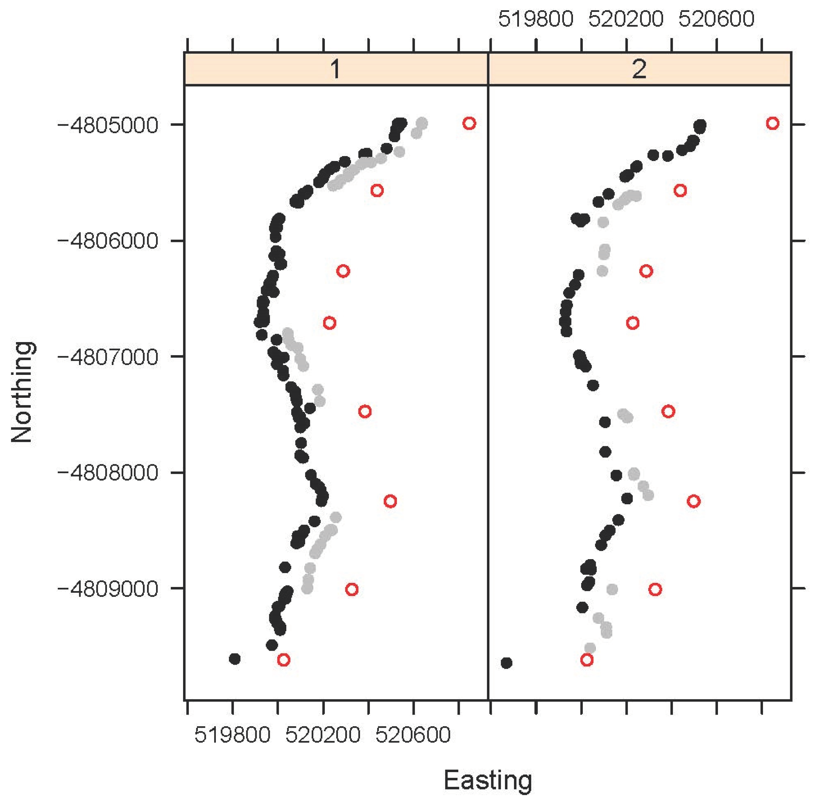

Table 1.
Results of the NB extended GLM fit to MBACI trial Tasmanian Pademelon roadkill counts quantifying the effect of the VF using LORP estimates.
Table 1.
Results of the NB extended GLM fit to MBACI trial Tasmanian Pademelon roadkill counts quantifying the effect of the VF using LORP estimates.
| Fixed effect | LORP estimates (SE, t-value) | Average LORP (SE, t-value) |
Percentage rate reduction | NB θ Estimate (Poisson deviance,DF) |
||
| 1 | 2 | 3 | ||||
| Rep | 0.326 (0.655, 0.50ns) |
-1.301 (0.804, -1.62ns) |
0.684 (0.807, 0.85ns) |
-0.097 (0.438, -0.22ns) |
9.2 | 4.8 (52.5**, 23) |
| Block | 0.254 (0.433, 0.59ns) |
-0.600 (0.620, -0.97ns) |
-0.172 (0.378, -0.46 ns) |
15.9 | 11.6 (47.7*, 27) |
|
ns P>0.05, * P <0.01, ** P <0.001 (one-sided tests).
Disclaimer/Publisher’s Note: The statements, opinions and data contained in all publications are solely those of the individual author(s) and contributor(s) and not of MDPI and/or the editor(s). MDPI and/or the editor(s) disclaim responsibility for any injury to people or property resulting from any ideas, methods, instructions or products referred to in the content. |
© 2024 by the authors. Licensee MDPI, Basel, Switzerland. This article is an open access article distributed under the terms and conditions of the Creative Commons Attribution (CC BY) license (https://creativecommons.org/licenses/by/4.0/).
Copyright: This open access article is published under a Creative Commons CC BY 4.0 license, which permit the free download, distribution, and reuse, provided that the author and preprint are cited in any reuse.


