
Submitted:
11 March 2024
Posted:
15 March 2024
You are already at the latest version
Abstract
This study was to identify clinical cancer biomarkers for recurrent gastric cancer survivors using artificial intel-ligence. From a hospital-based cancer registry database in Taiwan, the datasets of the incidence of recurrence and clinical risk features were included in 2476 gastric cancer survivors. We benchmarked Random forest with MLP, C4.5, AdaBoost, and Bagging algorithms on metrics and leveraged synthetic minority oversampling technique (SMOTE) for imbalanced dataset issues, cost-sensitive learning for risk assessment, and SHapley Additive ex-Planations (SHAP) for feature importance analysis in this study. Our proposed Random forest outperformed the other models with an accuracy of 87.9%, a recall rate of 90.5%, an accuracy rate of 86% and F1 of 88.2% on re-current category by a 10-fold cross-validation in a balanced dataset. We identified clinical features of recurrent gastric cancer, which are the top five features, stage, number of regional lymph node involvement, Helicobacter pylori, BMI(body mass index), and gender, which significantly affect the prediction model's output, are worth paying attention to in the following causal effect analysis. Using an artificial intelligence model, the risk factors for recurrent gastric cancer could be identified and cost-effectively ranked according to their feature importance. In addition, they should be crucial clinical features to provide physicians with the knowledge to screen high-risk patients in gastric cancer survivors as well.
Keywords:
Recurrent Gastric Cancer
; Random Forest
; SMOTE
; SHAP
; Cost-Sensitive Learning
1. Introduction
Gastric cancer is the fourth leading cause of cancer-related mortality worldwide, and its 5-year survival rate is less than 40%. H. pylori remains the leading cause of gastric cancer, which could vary from lymphomas, sarcomas, gastrointestinal stromal, and neuroendocrine tumors. With the development of biomarkers, more and more therapeutic strategies were designed to treat gastric cancer. However, early detection of recurrent gastric cancer can fundamentally improve a patient's survival, so it is essential to continue screening and monitoring even after it is disease-free. Early detection will allow physicians to provide early treatments for maximum benefit if cancer tumors recur in the stomach or elsewhere. Meanwhile, doctors and patients have always given importance to the issue of how to observe cancer recurrence with caution. In Taiwan, early detection and diagnosis have become feasible due to cancer screening promotion in recent years.
Artificial intelligence (AI), with the improvement of computing capacity, has been paid attention in the medical field. Machine learning (ML), which is part of AI, is critical in helping diagnosis and prognosis. Zhang et al. [1] developed a multivariate logistic regression analysis on a nomogram with radiomic signature and clinical risk factors to predict early gastric cancer recurrence. Liu et al. [2] used the Support Vector Machine classifier on the gene expression profiling dataset to predict gastric cancer recurrence and identify correlated feature genes. Zhou et al. [3] benchmarked the algorithms of random forest (RF), GBM, Gradient Boosting, Decision Tree, and Logistics. They concluded that the first four factors affecting postoperative recurrence of gastric cancer were body mass index (BMI), operation time, weight, and age.
We developed a risk prediction model for survivors of recurrent gastric cancer based on the above trends. In our study, we propose random forest [4] to develop a classifier and benchmark Multilayer Perceptron (MLP) [5], C4.5 [6], AdaBoost [7], and Bootstrap [8] Aggregation (Bagging [9]) algorithms in metrics. Regarding data preprocessing, we leverage Synthetic Minority Oversampling Technology (SMOTE) [10] oversampling against imbalanced dataset issues. For strategic risk assessment, we use cost-sensitive learning as a trade-off tool. Lastly, SHapley Additive exPlanations (SHAP) [11,12,13] are used for feature importance analysis from both global and local perspectives.
Finally, RF with SMOTE on this dataset can perform well, and SHAP can show reasonable interpretation and feature importance. Furthermore, the top five risk factors for recurrent gastric cancer were identified as stage, number of regional lymph node involvement, Helicobacter pylori, BMI, and gender.
2. Materials and Methods
2.1. Data Preparation and Machine Learning Models
A hospital cohort of 2476 patients diagnosed with gastric cancer survivors was enrolled in the Taiwan Cancer Registry (TCR) database from July 2008 to August 2020. Of them, 432 recurrent gastric cancers were used compared to 2,044 nonrecurrent survivors. All clinical figures recorded in this database were used to establish our predictive model. These clinical figures of gastric cancer survivors were used as the predictive features. In this study, the proposed process flow diagram is illustrated in Figure 1.
In step 1, we collected a recurrent gastric cancer dataset. For a better fit to our machine learning algorithms and TreeSHAP analysis, we encoded all our data into categorical variables in step 2. Due to the data imbalance between the nonrecurrence and recurrence categories, we balanced the dataset with the up-sampling method, SMOTE, for the minor category as step 3. One of our essential purposes is to understand the prediction behaviors of our trained model; therefore, we used 10-fold cross-validation without a data set split in step 4. RF is the focus that is used to compare with other baseline algorithms. In the final step, step 5, we further utilized model interpretation to observe feature importance and interactions.
RF is a kind of ensemble machine learning model based on Classification and Regression Trees (CART), Bagging, and random feature selection. This randomness design is suitable for preventing the over-fitting of other decision trees and tolerance against noise and outliers. The tree elements make decisions based on information gained to get automatic feature selection. Namely, RF has a built-in feature selection function within the training phase, so there is no need to prefilter all features by principal component analysis. We can also interpret that selection in the feature importance analysis section. The importance of RF features is a permutation approach that measures the decrease in prediction performance as we permute the value of the feature.
RF has become one of the most popular machine-learning algorithms based on the above properties. It has several advantages: 1) it is more accurate due to the ensemble approach, 2) it works without detailed hyperparameter setting and principal components analysis (PCA) preprocess, and 3) it computes efficiently and quickly. These are the reasons we chose RF as our backbone algorithm.
SMOTE (Synthetic Minority Oversampling Technology) is an oversampling algorithm proposed by Chawla et al. to improve overfitting. The method creates new randomly generated samples between samples of minority classes and their neighbors, which can balance the number among categories.
Cost-sensitive learning [14,15,16] is a training approach that considers the assigned costs of misclassification errors while training the model. This is closely related to the imbalanced dataset. We need different biases when we need other monitoring criteria in various risk management phases. The computing speed of RF is efficient, so we can easily integrate different cost biases for interested scenarios to get an overall picture.
SHAP analysis is an extension based on Shapley values, which is a game-theoretical method used to calculate the average of all marginal contributions in all coalitional combinations. Unlike the calculation of Shapley values, SHAP addresses the addictive features as a linear model. For a given feature set, SHAP values are calculated for each feature and added to a base value to give the final prediction.
TreeSHAP is proposed as a variant of SHAP for tree-based machine learning models, such as decision trees, RF, and gradient-boosted trees.
The importance of a SHAP feature is defined as the average of absolute SHAP values per feature for all instances. This focuses on the variance of model output, which is different from the importance of a permutation feature based on performance error. From it, we can know how the magnitude of model output changes, like likelihood or regression value, as we manipulate feature value, and it has nothing to do with performance, like accuracy or loss.
2.2. Dataset Sources
In the database of the Taiwan Cancer Registry, 17 variables are recorded as clinical potential features of recurrence, (1) gender, (2) age at diagnosis, (3) grade/differentiation, (4) tumor size, (5) number of regional lymph node involvement, (6) stage, (7) surgical margin involvement of the primary site, (8) radiation therapy, (9) chemotherapy, (10) BMI, (11) smoking, (12) chewing betelnut, (13) alcohol drink, (14) value of the CEA carcinoembryonic antigen, (15) CEA test of carcinoembryonic antigen, (16) Helicobacter pylori, (17) lymphatic or vascular. Therefore, the analysis aimed to identify the most critical risk features of these 17 predictors. The encoding and sample size features are organized in Figure 2. The original dataset has significantly imbalanced issues; that is, the minor category is about 20% of the majority. As mentioned above, the RF and decision trees will automatically select the best feature for each decision split. Therefore, we did not utilize PCA for dimensionality reduction.
2.3. Data Preprocessing
To better fit our machine learning algorithms and TreeSHAP analysis, we encode all of our data into categorical variables with an assigned integer. We also assign ordinal variables that are positive or higher intensity with larger integers so that TreeSHAP can show them well with a trend chart or dependence plot. However, most features have missing or unavailable values that have been encoded as middle or average rank to minimize possible bias on feature importance trends. That is, the moderate impact of the NA category should be between the maximum and minimum of ordinal values.
2.4. Dataset Balancing
Due to a significant imbalanced dataset, the model would tend to overfit the major categories and ignore the learning features of minorities. Generally, several approaches could overcome this learning bias due to target loss function design, such as assigning different weights for samples or categories in the loss function, assigning additional cost weight for prediction errors, resampling data by over or under-sampling, etc.
SMOTE is the method we use for over-sampling in this study. Instead of simply duplicating samples, we generate synthetic samples for minorities up to a quantity of the majority. It would select some nearby samples around a base sample of minority, randomly choose one neighbor, and randomly perturb one feature at a time within the distance between them.
2.5. 10-fold Cross-Validation
We use 10-fold cross-validation to prevent bias from a split of the whole dataset. Partition the complete dataset into ten equal-sized subgroups. Each time, a subgroup will be chosen as a holdout set, and the rest of the night subgroups are for training. At the end of 10 training rounds, an average performance of 10 models will be output.
We benchmark RF with MLP, C4.5, AdaBoost, and Bagging for the machine learning algorithm.
1. MLP: A classifier that uses backpropagation to learn a multilayer perceptron to classify instances.
2. C4.5: This algorithm develops a decision tree by splitting the value of the feature at each node, including categorical and numeric features. Calculate the information gain and use the feature with the highest gain as the splitting rule.
3. AdaBoost with C4.5: It is a part of the group of ensemble methods called boosting and adds newly trained models in a series where subsequent models focus on fixing the prediction errors made by previous models. In this study, we select C4.5 as the base classifier.
4. Bagging (Bootstrap Aggregation) with C4.5: This is an ensemble skill that uses the bootstrap sampling technique to form different sets of samples with replacement. We use C4.5 as a base classifier to derive the forest.
The RF classification model develops parallel decision trees that vote the category judgment for a given instance and output the final decision as a prediction. Cost-sensitive learning is essential in the case of risk management as we pursue better flexibility of trade-offs among metrics. For example, we may focus more on the recall rate of the recurrence category by loosening the performance of the precision rate. In this part, we assign different costs of the false negative error of recurrence categories 1, 2, 3, and 5 but keep the false positive error cost at 1.
In our study, we set the recurrence category as positive and then evaluated the metrics. True Positive (TP): number of positive instances predicted as positive. Negative (TN): number of negative instances predicted as negative. False Positive (FP): number of negative instances predicted as positive. False Negative (FN): number of positive instances predicted as negative. Accuracy: (TP+TN)/(TP+TN+FP+FN). Precision: TP/(TP+FP). Recall: TP/(TP+FN). F1-score: 2×(Recall × Precision) / (Recall + Precision). False Positive Rate: FP/(FP+TN). True Positive Rate: TP/(TP+FN). The ROC curve (receiver operating characteristic curve) uses the True Positive Rate as the y-axis and False Positive Rate as the x-axis and plots points with corresponding thresholds.
2.6. Interpretability in Machine Learning Models
We review the importance of features using two approaches, RF and SHAP. The former is a single-feature permutation approach to observe model performance impact, whereas the latter is flexible in observing main features and the interaction effects regarding model output.
Concerning SHAP, we use global interpretability plots. The feature importance plot lists the importance of all features in ascending and color bars with positive or negative correlation coefficients. The Bee Swarm plot for feature importance provides vibrant SHAP value and output impact direction information of individual points in rich colors that can help users get critical insights quickly. The dependence plot helpfully shows the correlations and interactions between the two features and the SHAP value trends.
The local interpretability plot, the waterfall plot, is designed to demonstrate explanations for individual instances.
3. Results
3.1. Prediction Performance
The balanced dataset has original major category 2044 instances and oversampled minor category 2044 instances. The 10-fold cross-validation is used for performance checks. Table 1 summarizes the comparison of different algorithms, including MLP, C4.5, AdaBoost with C4.5, Bagging with C4.5, and RF. RF has a metric outperformance of F1 of 88.2%, ROC area of 95.2%, PRC of 95.4%, and 87.9% for the recurrence category. First, MLP shows better metric performance than C4.5 as a benchmark between the numerical-base algorithm and the categorical-base decision tree algorithm. Second, from the evidence that RF significantly surpasses the C4.5 and Bagging sets, we believe that the main improvement is from the randomness design of bootstrap subsampling and the choice of feature for splitting node. Third, compared with AdaBoost, the independent trees of RF show better ensemble synergy than the boosting ensemble that arranges trees of the forest in series.
From the comparison of the ROC curves in Figure 3(a), RF has the largest 0.952 area, which means that the trade-off between TPR and FPR through threshold setting is relatively better than others, while C4.5 is the worst.
In Table 2, we can see that the recall rate increases (that is, 90.5% to 96.1%) if we increase the penalty cost on the FN (false negative) error of the recurrence category but keep the FP error cost as one precision rate (that is, 86% to 74.2%) and the overall accuracy (that is, 87.9% to 81.4%) are compromised accordingly. This policy scenario means that we hope that potential recurrence patients are labeled as much as possible, with acceptable results of FP (false positive) patient misclassification. Figure 3(b) shows no noticeable difference between different costs.
3.2. Interpretability
Before diving into the explanation of features, we need to understand that model interpretability is not always equal to causality. It is essential to address that SHAP values do not provide causality but insights into how the model behaves from data learning.
First, we use RF to observe global characteristics. Figure 4(a) shows that F-6/F-5/F-2 are the top three impact features. The SHAP value in Figure 4(b) shows more information. First, it agrees that F-6 and F-5 have a critical and positive impact, which means that higher features bring bigger recurrence probability; meanwhile, F-2 falls to 6th with a negative impact. Moreover, the F-16 also runs up to the third feature with a negative impact. The red bars have a positive correlation coefficient.
Next, we could further investigate the SHAP distribution of all instances in Figure 5(a); the bee swarm plot, F-6, and F-5 show higher feature value instances (i.e., red points contribute positive SHAP values), mostly with higher SHAP values. On the contrary, the feature values negatively correlate with the SHAP values (i.e., blue points contribute positive SHAP values).
Figure 5(b), the breakdown of the dependence plot, shows the SHAP value in relation to main and interaction effects if we want to investigate the interaction between features further. The on-diagonal values are the main effect, whereas the off-diagonal values are interactions. From the upper left corner of Figure 5(b), we can see that interactions between F-5/F-6 would bring a negative SHAP value. In other words, F-5/F-6 would have positive main SHAP values, respectively, from the diagonal, but the off-diagonal interaction value would somehow decrease the main values.
Global interpretation shows correlations between features and prediction in all samples, which cannot clearly explain the prediction specific to a specific sample. Figure 6(a) locally indicates the breakdown of individual SHAP values of recurrent instances; from that, we can clearly see how those feature forces bring the prediction probability f(x) up to 1. In contrast, Figure 6(b) nonrecurrence case shows reverse forces bring f(x) down to 0. Most importantly, in everyday work, we can analyze individual patients with RF and local SHAP analysis, as shown in Figure 6, to understand the impacts of all features.
4. Discussion
More than 60% of gastric cancer survivors experienced recurrence after curative resection for gastric cancer, especially within two years after surgery. The risk factors for the recurrence patterns of different clinical or pathological factors were supposed to lead to recurrences of gastric cancer [17]. However, how to predict the recurrence of gastric cancer is still not common.
Lo et al. [18] found that the most critical risk factors for recurrence in early gastric cancer are lymph node status and the size of the mucosal tumor. Compared to advanced gastric cancer, the prognosis for patients with early gastric cancer is excellent. In our study, the result of F-4 (tumor size) / F-5 (number of regional lymph node involvement) / F-6 (cancer stage) with positive SHAP values is similar to their report.
In 2009, Tokunaga et al. [19] described that a 5-year survival rate after curative gastrectomy is better in overweight than non-overweight patients. The overweight as an independent prognostic factor revealed in patients with early gastric cancer was revealed; however, the reason was not yet determined. With our prediction model, F-10(BMI) is the fourth leading feature with a negative impact on the recurrence of gastric cancer. The results were similar.
In 2020, Zheng et al. [20] identified that the pathological tumor (pT) stage and the pathological nodal (pN) stage were significantly associated with the prognosis of stage I gastric cancer. The postoperative chemotherapy adjuvant might help improve the outcomes of high-risk patients. In our study, more clinical figures were collected and divided into subgroups for analysis. F-6 (cancer stage) is the leading risk factor, followed by F-5 (number of regional lymph node involvement). A similar result was concluded.
Helicobacter pylori, which is not only the leading risk factor for gastric cancer but also a high risk of recurrence, colonizes the gastric mucosa and induces persistent chronic gastric inflammation. [21,22] Patients with a genotype of high IgG1 level will have a higher risk of recurrence than patients with other genotypes. Our study demonstrated that SSF3(Helicobacter pylori) is the third leading feature for the recurrence of gastric cancer.
Artificial intelligence has become a workhorse for cancer diagnosis and prognosis with unprecedented accuracy, which is more powerful than traditional statistical analysis [23]. Chang et al. used a stacked ensemble-based classification model to predict the second primary cancer of head and neck cancer survivors by clinical features [24]. With artificial intelligence, a prediction model is possible to figure out clinical risk features, which will help clinicians screen cancer survivors before recurrence occurs.
In this study, we explore data mining using the machine learning algorithm RF on the imbalanced dataset. Furthermore, we utilize SMOTE to oversample the minority to balance and prevent the model from being biased too much on the original majority of non-recurrent instances. Regarding metric performance, RF shows better prediction capability than MLP, C4.5, AdaBoost, and Bagging. The prediction performance metrics can reach an overall accuracy of 87.9%, a recall rate of 90.5%, a precision rate of 86%, and F1 88.2% of recurrent category by 10-fold cross-validation in the balanced dataset.
Regarding cost-sensitive learning, as we increase the cost of FN, the recall rate can improve from 90.5% to 96.1%. Meanwhile, the precision rate is compromised from 86% to 74.2%, and the accuracy from 97.9% to 82.4%. Cost learning is a quick way of conventional machine learning to assess risk, while we intend to switch between different policies.
From SHAP value interpretation analysis, we can get insights into how models make a decision based on features and the interaction between correlated features. Identified top 5 features are F-6(Cancer stage), F-5(Number of regional lymph node involvement), SSF3(Helicobacter pylori), BMI, and gender. But remember that model interpretation is for model behavior analysis, not equal to causal effect analysis. The model learns from complicated correlations within the dataset, as shown in Figure 5(b), and looks for the best choice to optimize an objective function.
We have some limitations in this study. Firstly, TCR data was collected from different hospitals and periods. Some features have a significant number of missing values, such as lymphatic or vascular invasion. This situation may bias real trends if this feature contributes a significant SHAP value. We need to pay attention once we interpret this feature.
5. Conclusions
In conclusion, RF is the best classifier of prediction capability in our study. Cost-sensitive learning could be achieved with an improvement in the recall rate from 90.5% to 96.1%, a compromised precision rate from 86% to 74.2%, and accuracy from 97.9% to 82.4%. Mostly, F-6 (cancer stage), F-5 (number of regional lymph node involvement), SSF3(Helicobacter pylori), BMI, and gender were the leading impact factors for recurrent gastric cancer. They will be helpful for physicians in detecting high-risk patients early in gastric cancer survivors. This study used data from the Taiwan Cancer Registry Database to estimate retrospective clinical figures of gastric cancer at diagnosis and to evaluate the association with gastric cancer recurrence after the launch of targeted therapies. Despite these limitations, this study should provide an essential basis for further research.
Author Contributions
Conceptualization, C.-C.Chang, W.-C.Ting and H.-C.L.; Methodology, C.-C.Chang and H.-C.L.; Validation, C.-C.Chang, C.-C.Chen; Formal analysis, C.-C.Chang and H.-C.L.; Writing—original draft, C.-C.Chen; W.-C.Ting ; H.-C.L. and S.-F.Y.; Writing—review & editing, C.-C.Chang, H.-C.L., W.-C.Ting and C.-C.Chen; Visualization, H.-C.L. and S.-F.Y.; Supervision, C.-C.Chang. All authors have read and agreed to the published version of the manuscript.
Funding
This study was funded by a research grant from Taiwan’s Ministry of Science and Technology (112-2321-B-040 -003-). Chung Shan Medical University Hospital Foundation grant:CSH-2023-C-029.
Institutional Review Board Statement
This study was approved by the Institutional Review Board of the Chung Shan Medical University Hospital (IRB no. CS2-20114).
Informed Consent Statement
Not applicable.
Data Availability Statement
Data are available from the Institutional Review Board of Chung Shan Medical University Hospital for researchers who meet the criteria for access to confidential data. Requests for the data may be sent to the Chung Shan Medical University Hospital Institutional Review Board, Taichung City, Taiwan (e-mail: irb@csh.org.tw).
Conflicts of Interest
The authors declare no conflict of interest.
References
- Zhang W, Fang M, Dong D, Wang X, Ke X, Zhang L, et al. Development and validation of a CT-based radiomic nomogram for preoperative prediction of early recurrence in advanced gastric cancer. Radiother Oncol. 2020, Apr;145:13-20. [CrossRef]
- Liu B, Tan J, Wang X, Liu X. Identification of recurrent risk-related genes and establishment of support vector machine prediction model for gastric cancer. Neoplasma. 2018, Mar 14;65(3):360-366. [CrossRef]
- Zhou C, Hu J, Wang Y, Ji MH, Tong J, Yang JJ, et al. A machine learning-based predictor for the identification of the recurrence of patients with gastric cancer after operation. Sci Rep. 2021, Jan 15;11(1):1571. [CrossRef]
- Breiman, L. Random forest. Machine Learning. 2001, 45, 5–32. [Google Scholar] [CrossRef]
- Haykin, S. Neural networks: a comprehensive foundation. Prentice Hall PTR; 1994.
- Salzberg, SL. C4.5: Programs for Machine Learning by J. Ross Quinlan. Morgan Kaufmann Publishers, Inc., 1993. Mach Learn 16, 1994, 235–240. [CrossRef]
- Yoav Freund, Robert E Schapire. Experiments with a New Boosting Algorithm. International Conference on Machine Learning; Bari; 1996 July 3-6; 1996. p.148-156.
- Efron B, Tibshirani RJ. An Introduction to the Bootstrap. Chapman and Hall, New York. 1993.
- Breiman, L. Bagging predictors. Machine Learning. 2004, 24, 123–140. [Google Scholar] [CrossRef]
- Chawla N, Bowyer K, Hall LO, Kegelmeyer WP. SMOTE: Synthetic Minority Over-sampling Technique. J. Artif. Intell. Res. 2002, 16, 321–357. [CrossRef]
- Lundberg SM, Lee SA. Unified Approach to Interpreting Model Predictions. 2017. [CrossRef]
- Lundberg SM, Erion G, Chen H, DeGrave A, Prutkin JM, Nair B, et al. From Local Explanations to Global Understanding with Explainable AI for Trees. Nat Mach Intell. 2020, Jan;2(1):56-67. [CrossRef]
- Lundberg SM, Nair B, Vavilala MS, Horibe M, Eisses MJ, Adams T, et al. Explainable machine-learning predictions for the prevention of hypoxemia during surgery. Nat Biomed Eng. 2018, Oct;2(10):749-760. [CrossRef]
- Krawczyk B, Wozniak M, Schaefer G. Cost-sensitive decision tree ensembles for effective imbalanced classification. Appl. Soft Comput. 2014, 14, 554–562.
- C Seiffert, TM Khoshgoftaar, JV Hulse, A Napolitano. A Comparative Study of Data Sampling and Cost Sensitive Learning. 2008 IEEE International Conference on Data Mining Workshops; 2008, p. 46-52.
- Thai-Nghe N, Gantner Z, Schmidt-Thieme L. Cost-sensitive learning methods for imbalanced data. The 2010 International Joint Conference on Neural Networks (IJCNN). 2010, p. 1-8.
- Liu D, Lu M, Li J, Yang Z, Feng Q, Zhou M, et al. The patterns and timing of recurrence after curative resection for gastric cancer in China. World J Surg Oncol. 2016, Dec 8;14(1):305. [CrossRef]
- Lo SS, Wu CW, Chen JH, Li AF, Hsieh MC, Shen KH, et al. Surgical results of early gastric cancer and proposing a treatment strategy. Ann Surg Oncol. 2007, Feb;14(2):340-7. [CrossRef]
- Tokunaga M, Hiki N, Fukunaga T, Ohyama S, Yamaguchi T, Nakajima T. Better 5-year survival rate following curative gastrectomy in overweight patients. Ann Surg Oncol. 2009, Dec;16(12):3245-51. [CrossRef]
- Zheng D, Chen B, Shen Z, Gu L, Wang X, Ma X, et al. Prognostic factors in stage I gastric cancer: A retrospective analysis. Open Med (Wars). 2020, Aug 3;15(1):754-762. PMID: 33336033; PMCID: PMC7712043. [CrossRef]
- Seeneevassen L, Bessède E, Mégraud F, Lehours P, Dubus P, Varon C. Gastric Cancer: Advances in Carcinogenesis Research and New Therapeutic Strategies. Int J Mol Sci. 2021, Mar 26;22(7):3418. [CrossRef]
- Sato M, Miura K, Kageyama C, Sakae H, Obayashi Y, Kawahara Y, et al. Association of host immunity with Helicobacter pylori infection in recurrent gastric cancer. Infect Agent Cancer. 2019, Feb 11;14:4. [CrossRef]
- Huang S, Yang J, Fong S, Zhao Q. Artificial intelligence in cancer diagnosis and prognosis: Opportunities and challenges. Cancer Lett. 2020, Feb 28; 471:61-71. [CrossRef]
- Chang CC, Huang TH, Shueng PW, Chen SH, Chen CC, Lu CJ, et al. Developing a Stacked Ensemble-Based Classification Scheme to Predict Second Primary Cancers in Head and Neck Cancer Survivors. Int J Environ Res Public Health. 2021, Nov 27;18(23):12499. [CrossRef]
Figure 1.
The proposed process flow diagram of this study.
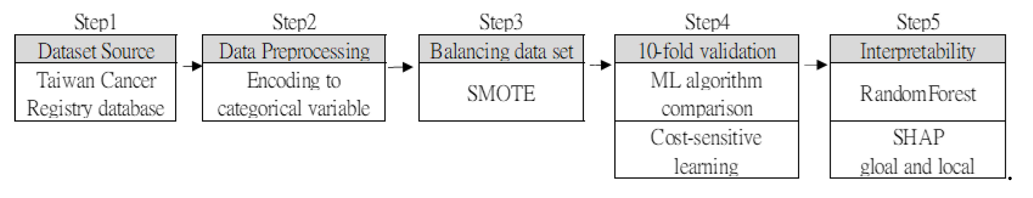
Figure 2.
The dataset features with encodings and sample sizes were demonstrated in our predicting analysis.
Figure 2.
The dataset features with encodings and sample sizes were demonstrated in our predicting analysis.
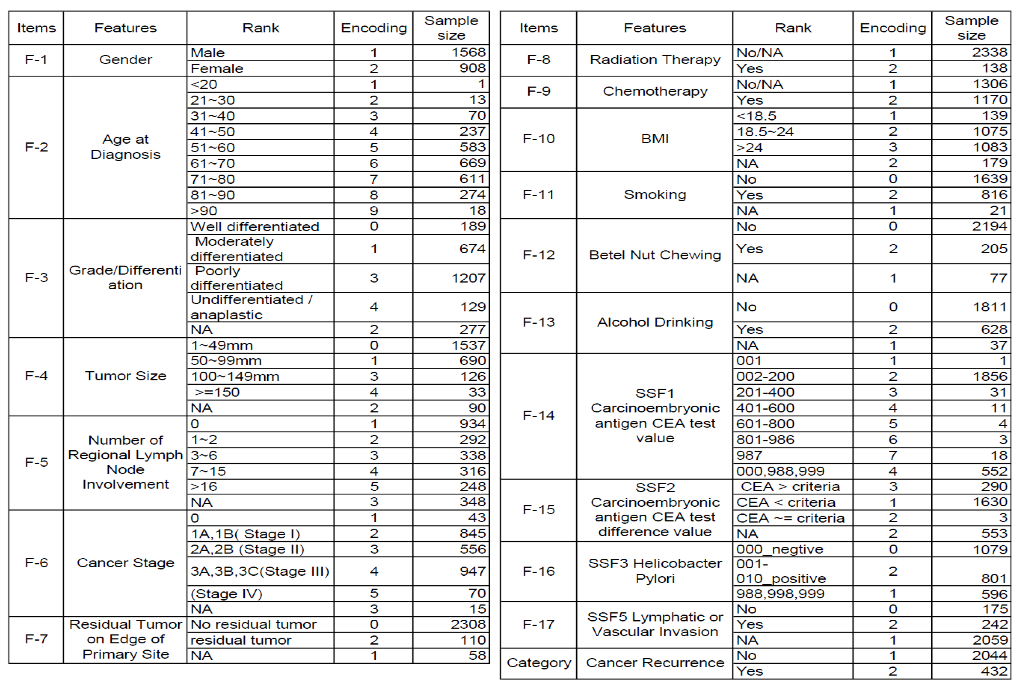
Figure 3.
ROC curves for (a)different algorithms, (b) Random forest with different FN costs.
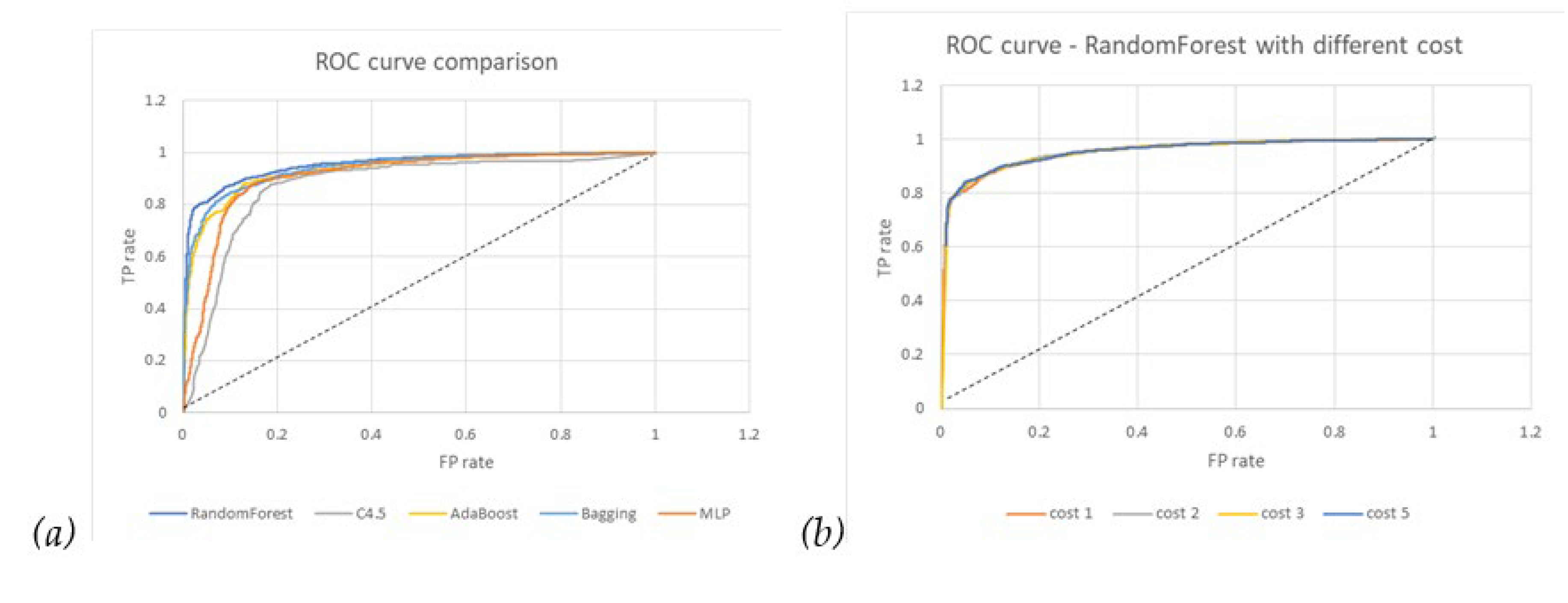
Figure 4.
The clinical features were ranked by their feature importance. (a) Random forest feature importance and (b) SHAP value (Red: positive impact; Blue: negative impact.).
Figure 4.
The clinical features were ranked by their feature importance. (a) Random forest feature importance and (b) SHAP value (Red: positive impact; Blue: negative impact.).
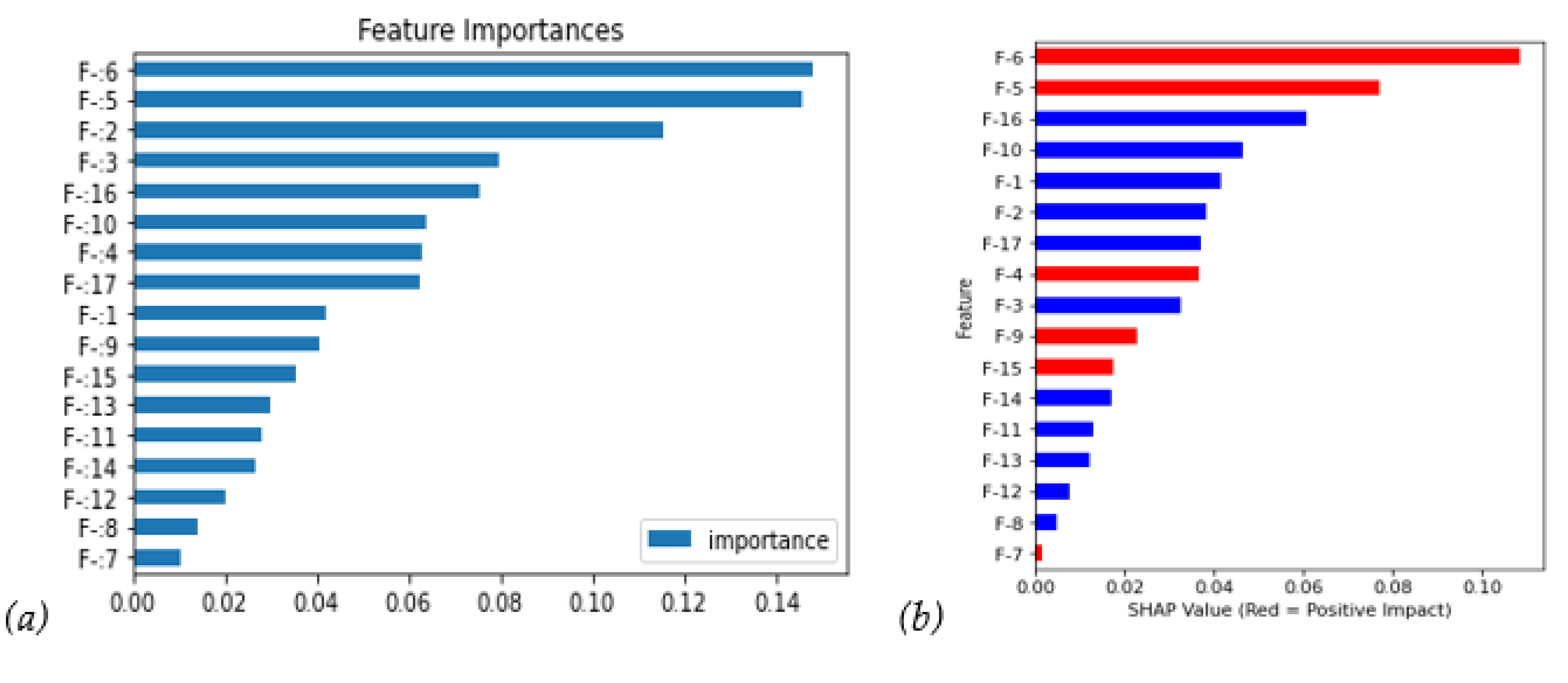
Figure 5.
(a) Bee swarm plot and (b) Dependence plot. With SHAP interaction matrix between the top 10 clinical features.
Figure 5.
(a) Bee swarm plot and (b) Dependence plot. With SHAP interaction matrix between the top 10 clinical features.
Figure 6.
Waterfall plot. Two examples of local interpretation are (a) the recurrent case and (b) the non-recurrent case. f (x) is the expectation (that is, the average predictions of all instances).
Figure 6.
Waterfall plot. Two examples of local interpretation are (a) the recurrent case and (b) the non-recurrent case. f (x) is the expectation (that is, the average predictions of all instances).
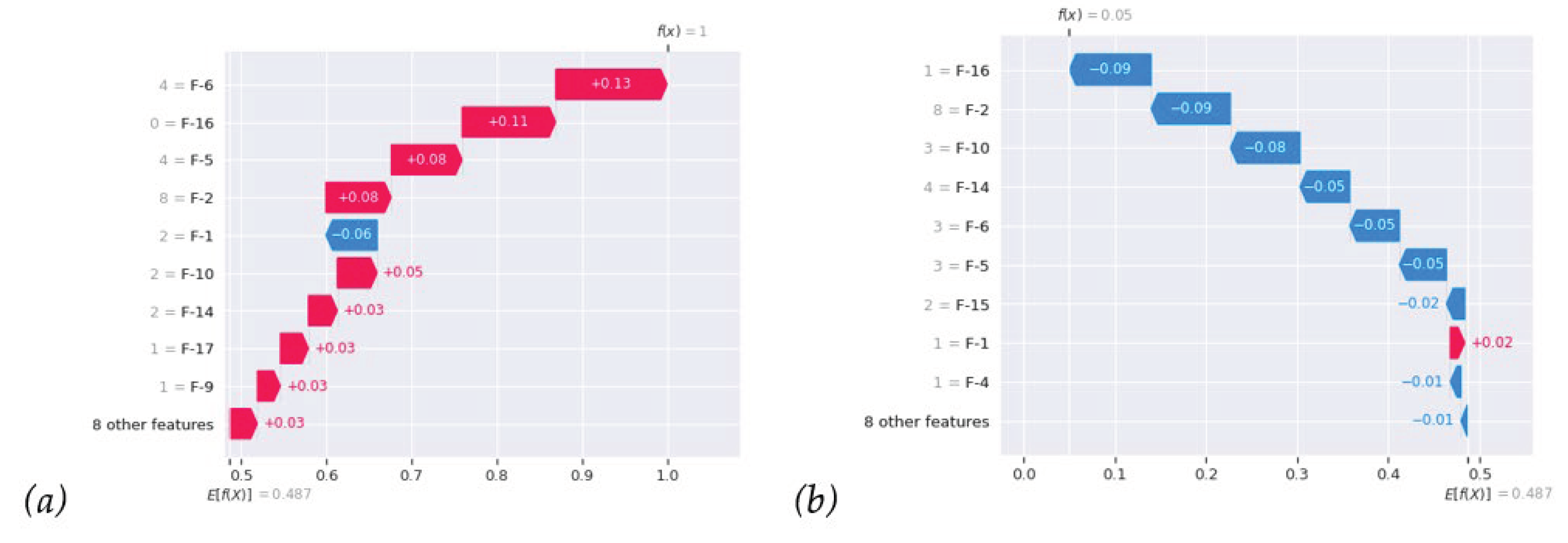

Table 1.
Comparison of classification performance for different algorithms.
| Cost of FN | TP rate | FP rate | Precision | Recall | F1 score | ROC area | PRC area | Accuracy | Category |
|---|---|---|---|---|---|---|---|---|---|
| 1 | 0.853 | 0.095 | 0.899 | 0.853 | 0.875 | 0.952 | 0.945 | 0.879 | Non- Recurrence |
| 0.905 | 0.147 | 0.860 | 0.905 | 0.882 | 0.952 | 0.954 | Recurrence | ||
| 2 | 0.799 | 0.066 | 0.924 | 0.799 | 0.857 | 0.954 | 0.948 | 0.866 | Non- Recurrence |
| 0.934 | 0.201 | 0.823 | 0.934 | 0.875 | 0.954 | 0.955 | Recurrence | ||
| 3 | 0.743 | 0.058 | 0.928 | 0.743 | 0.825 | 0.953 | 0.947 | 0.842 | Non- Recurrence |
| 0.942 | 0.257 | 0.785 | 0.942 | 0.857 | 0.953 | 0.953 | Recurrence | ||
| 5 | 0.666 | 0.039 | 0.945 | 0.666 | 0.782 | 0.953 | 0.947 | 0.814 | Non- Recurrence |
| 0.961 | 0.334 | 0.742 | 0.961 | 0.838 | 0.953 | 0.954 | Recurrence |
TP : True positive; FP : False positive; FN: False negative.
Table 2.
Comparison of the performance of the random forest classification performance for different costs.
Table 2.
Comparison of the performance of the random forest classification performance for different costs.
| Algorithm | TP rate | FP rate | Precision | Recall | F1 score | ROC area | PRC area | Accuracy | Category |
|---|---|---|---|---|---|---|---|---|---|
| MLP | 0.835 | 0.112 | 0.882 | 0.835 | 0.858 | 0.909 | 0.91 | 0.862 | Non-Recurrence |
| 0.888 | 0.165 | 0.843 | 0.888 | 0.865 | 0.909 | 0.883 | Recurrence | ||
| C4.5 | 0.812 | 0.123 | 0.869 | 0.812 | 0.839 | 0.874 | 0.849 | 0.844 | Non- Recurrence |
| 0.877 | 0.188 | 0.823 | 0.877 | 0.849 | 0.874 | 0.826 | Recurrence | ||
| AdaBoost C4.5 | 0.859 | 0.115 | 0.882 | 0.859 | 0.87 | 0.933 | 0.924 | 0.872 | Non- Recurrence |
| 0.885 | 0.141 | 0.863 | 0.885 | 0.873 | N0.933 | 0.937 | Recurrence | ||
| Bagging C4.5 | 0.829 | 0.111 | 0.882 | 0.829 | 0.855 | 0.941 | 0.932 | 0.859 | Non- Recurrence |
| 0.889 | 0.171 | 0.839 | 0.889 | 0.863 | 0.941 | 0.945 | Recurrence | ||
| Random Forest | 0.853 | 0.095 | 0.899 | 0.853 | 0.875 | 0.952 | 0.945 | 0.879 | Non- Recurrence |
| 0.905 | 0.147 | 0.860 | 0.905 | 0.882 | 0.952 | 0.954 | Recurrence |
Disclaimer/Publisher’s Note: The statements, opinions and data contained in all publications are solely those of the individual author(s) and contributor(s) and not of MDPI and/or the editor(s). MDPI and/or the editor(s) disclaim responsibility for any injury to people or property resulting from any ideas, methods, instructions or products referred to in the content. |
© 2024 by the authors. Licensee MDPI, Basel, Switzerland. This article is an open access article distributed under the terms and conditions of the Creative Commons Attribution (CC BY) license (http://creativecommons.org/licenses/by/4.0/).
Copyright: This open access article is published under a Creative Commons CC BY 4.0 license, which permit the free download, distribution, and reuse, provided that the author and preprint are cited in any reuse.


