Submitted:
17 February 2024
Posted:
20 February 2024
You are already at the latest version
Abstract
The ferrocell is an optical viewing device that interacts with a magnetic field and one or more light
sources to produce a real-time visual light display. Although this device has been extensively studied
by several researchers, a proper computer simulation replicating this optical effect has not yet been
presented. Using numerical methods and the law of reflection, a computer simulation was developed
that shows that the light patterns as seen in the ferrocell are primarily caused by light reflections
off the ferrofluid nano-particles that self organize into needle-like filaments and align along magnetic
flux lines in the presence of a magnetic field.
Keywords:
Ferrocell
; Magnetism
; Simulation
1. Introduction
The ferrocell device, invented by Timm Vanderelli (Patent number: US-8246356), consists of two main components: 1) a ferrolens and 2) a light source. The ferrolens is best described as a Hele-Shaw cell, (two closely spaced transparent parallel plates with fluid between them). In a typical ferrolens, a ferrofluid mixture is sandwiched between two optically flat pieces of glass. The visual effects appear when a magnet is placed in the vicinity of the lens illuminated with one or more light sources. Tufaile et al have identified these visual effects as being caused by reflection analogous to what happens in atmospheric optics, [1,2]. Thus, in our simulations, the law of reflection was used as a starting point. Since “what the observer sees” is highly dependent on the position of the magnet, the lights, and the observer with respect to the ferrolens, all of these parameters were taken into consideration in the computer simulation. The results clearly show that reflection is the primary cause of the patterns as seen in the ferrocell. Scattering also plays a role but only in relation to the “fuzziness” of the light patterns. Here, scattering is defined as a deviation from the ideal path of the reflected light. A first order implementation of scattering is included in the simulation. In the research presented herein, numerical methods and computer simulations were used to accurately model a variety of magnetic configurations and ferrocell displays.
2. Scope
The simulations presented in this paper are limited to the thin layer of ferrous particles sandwiched between the two pieces of glass and do not incorporate the effects of the glass itself or the fluid mixture. The purpose of this research was to develop a simulation to accurately predict and reproduce the patterns that the observer would see as a function of the applied magnetic field, the observer’s location, the plane of ferrofluid, and the location of the light sources.
3. Background
Ferrofluid is a colloidal solution of magnetic nano-particles suspended in a carrier fluid such as water or oil or some other organic solvent. Each nanoparticle (around 10 nm in size) consists of a ferrimagnetic or ferromagnetic core coated with a surfactant (e.g., oleic acid) to inhibit aggregation. In the ferrocell, the ferrofluid is further diluted using a light oil (eg. WD-40, Baby Oil) and placed in a thin layer between two pieces of optically flat glass.
Upon application of an external magnetic field, the nanoparticles between the two pieces of glass self-organize into needle-like filaments which are in the order of 100 m in length [5]. These micro-needles then align with the magnetic field to minimize dipolar interactions as seen under the microscope in Figure 1. The light from the light source (LED, laser etc.) reflects off these filaments and into the eye (or camera) to produce interesting patterns that change in real-time as the magnet is moved around.
Specular reflections are described by the law of reflection giving the reflection vector () as a function of the incident vector () and the surface normal vector () at the reflection point, with the constraint that . In other words when the two vectors are perpendicular to each other.
It is well known that light striking a thin edge results in an optical phenomenon know as a Keller’s cone [3]. A Keller’s cone can also be described as all valid reflection values of for light striking an extremely thin cylinder at some angle without the aforementioned constraint. Keller’s geometric diffraction theory extends beyond the concepts of reflection and refraction with the addition of diffraction [4]. For a thin cylinder, incident light is also diffracted around the obstruction producing interference patterns as noted by Tufaile et al [5]. The simulation presented herein is primarily targeting Keller’s cone and not the interference patterns, which contribute minimally to the light patterns seen in the ferrocell.
The needle-like filaments that form upon the application of the magnetic field can be considered as micro-cylinders with the long axis aligned with the magnetic field. Incident light reflects off the cylinders and when the observer’s eye intersects the resultant Keller cone, the observer will perceive a bright spot. Some deviations from the predicted reflections (a.k.a. scattering) is also involved. From this, we see that the lines observed in the ferrocell are all the points where (1) holds without the constraint that . Here, is the displacement vector from a light to the micro-cylinders, and is the displacement vector from the cylinders to the observer’s eye.
4. Methods
4.1. Experimental
The ferrolens used in these experiments was created using two optically flat glass disks as depicted in Figure 2. A few drops of a fluid mixture consisting of 1 part ferrofluid (EFH series) to 1 part light oil was placed in the center of one glass disk. The other glass disk is then placed on top of the first causing the fluid to spread between the two pieces of glass. The optical flatness of the glass allows for a very thin layer to form, in the order of 10 m. A magnet or array of magnets is then placed under the ferrocell and one or more light sources are used to illuminate the lens. A camera is positioned above the ferrocell to capture the patterns that form when the magnetic configuration is in place.
4.2. Simulation
Figure 3 a flowchart of the simulation software. The simulation starts with a structured grid of coordinates to represent position vectors within the ferrocell film. Given a magnet or set of magnets of specific geometry, the magnetic field is then computed by defining a 3D structured grid with position and normalised magnetic moment such that the field at a given point is the sum of the field due to each moment in the magnet,
where . The direction of each micro-cylinder’s long axis is then given by the unit vector at position . For simplicity, a software package called Magpylib was utilized for these calculations [7]. The positions of the lights, , are then taken into consideration, as well as the position of the observer . With known incident and reflection vectors, the normal vector is recovered in equation 1 by normalising the difference between the reflection vector and incident vector:
To calculate the normal vector, , the incident vector and reflection vector are substituted into equation 3. To be consistent with equation 1, the condition must hold for a point to appear illuminated to the observer. Since numerical methods are limited in precision, it is unlikely that a simulation would return a situation where these conditions hold. However, the micro-cylinders in an experimental system have finite roughness and not a perfect circular cross-section. In addition, the light sources and the observer are not point-like. These imperfections allow us to relax the condition such that a point is considered illuminated if where T represents some threshold value to expand the range with which we can consider the result valid. This can be considered as a first order implementation of scattering.
5. Results
Figure 4 shows how a single light source interacts with the ferrolens in the presence of a magnet. The simulation (middle image) is calibrated to the experimental setup on the left as specified in this figure. Notice that the loop of light appears to intersect a point at the center of the LED. This is the light source that is being targeted in the simulation. The light emitted at the front and back ends of the LED are not being simulated as they do not contribute significantly to the light patterns seen in the ferrocell. Notice that the curved light line predicted by the simulation accurately matches the egg shaped curve as seen in the ferrocell.
In Figure 5, there are 36 lights (a repeating pattern of red, green, blue and yellow) surrounding a 5cm diameter ferrocell with a cylindrical magnet in polar view (N-pole up) under the lens. The simulation on the right was calibrated to the experimental setup on the left. The magnet is highlighted in grey. Notice that the central black region in the simulation does not correspond to the outer boundary of the magnet. Instead, it corresponds to a smaller darker circular region in the center of the magnet as can be seen in the ferrocell image. Here, the simulation accurately predicts both the trajectories of the curved light lines as well as the central dark region as seen in Figure 5.
In Figure 6 there are 36 lights (white only) surrounding a 10cm diameter ferrolens. A large cube magnet is placed under the ferrocell in a dipole orientation (magnetic poles are to the left and right). The simulation on the right is calibrated to the experimental setup on the left. In this simulation, you can see that the light lines match very well to what is seen in the ferrocell as well as the locations and shapes of the dark voids near either pole.
In Figure 7 there are 36 lights (red, green blue and white) surrounding a 5cm diameter ferrocell with two cylindrical magnets in a quadrupole configuration. As usual, the simulation on the right was calibrated to the experimental setup on the left. Here, the correlation between the experimental setup and the simulation is quite good. In the simulation however, some artifacts are observed in the image that are not seen in the ferrocell. This problem was fixed by placing a thin black barrier between the magnet and the ferrocell thus hiding the magnet from view. Also, since we are not simulating the effects of the glass, the top glass disk was removed from the ferrocell. After removing the glass and hiding the magnet, the extra features seen in the simulation were also seen in the ferrocell as depicted in Figure 8. This was a good test of the algorithm as it was able to make a prediction that was subsequently replicated in the experiment.
Figure 9 shows a close up of the crossing lines in both the ferrocell (left) and the simulation (right). Here, when the red lines and green lines intersect, yellow is observed; when green and blue intersect, cyan is observed; when red and blue intersect, magenta is observed and when yellow and blue intersect, white is observed. This additive colour mixing from standard light theory [8] can be seen in both the ferrocell image and the simulation.
6. Conclusion
Computer simulations were used to accurately replicate the visual effects of the ferrocell using various magnetic configurations. These simulations clearly show that the light patterns, as seen in the ferrocell, are primarily caused by light reflections off the needle-like filaments that form and align with the magnetic flux lines of the magnet when placed in the vicinity of a ferrocell. All of the main features of the ferrocell display, including the paths of the light curves, the locations and shapes of the dark voids near the poles and the additive mixing of colours, can be simulated using the law of reflection, standard magnetic theory and standard light theory. The ferrocell shows you what the magnetic field would look like if light could reflect off of the magnetic field lines.
Acknowledgments
Special thanks to Timm Vanderelli for lending he his ferrocell light box which was used for many of experiments presented in this paper, to A.B. for the Python simulation code that made all of this possible, to László Vadkerti for his images of ferrofluid under the microscope.
References
- Tufaile, Alberto, Timm A. Vanderelli, and Adriana Pedrosa Biscaia Tufaile. “Observing the jumping laser dogs.” Journal of Applied Mathematics and Physics 4, no. 11 (2016): 1977-1988. [CrossRef]
- Tufaile, Alberto, Michael Snyder, Timm A. Vanderelli, and Adriana Pedrosa Biscaia Tufaile. “Jumping Sundogs, Cat’s Eye and Ferrofluids.” Condensed Matter 5, no. 3 (2020): 45. [CrossRef]
- Senior, T. B. A., and P. L. E. Uslenghi. “Experimental detection of the edge-diffraction cone.” Proceedings of the IEEE 60, no. 11 (1972): 1448-1448. [CrossRef]
- Keller, Joseph B. “Geometrical theory of diffraction.” Josa 52, no. 2 (1962): 116-130. [CrossRef]
- Tufaile, Alberto, Michael Snyder, and Adriana Pedrosa Biscaia Tufaile. “Horocycles of Light in a Ferrocell.” Condensed Matter 6, no. 3 (2021): 30. [CrossRef]
- http://www.pic2mag.com/.
- Ortner, Michael, and Lucas Gabriel Coliado Bandeira. “Magpylib: A free Python package for magnetic field computation.” SoftwareX 11 (2020): 100466. [CrossRef]
- https://en.wikipedia.org/wiki/Additive_color.
Figure 1.
Ferrocell under a microscope. Left: Ferrofluid in the absence of a magnet. Right: Ferrofluid in the presence of a magnet. Longer filaments in the order of 100 microns in length.
Figure 1.
Ferrocell under a microscope. Left: Ferrofluid in the absence of a magnet. Right: Ferrofluid in the presence of a magnet. Longer filaments in the order of 100 microns in length.
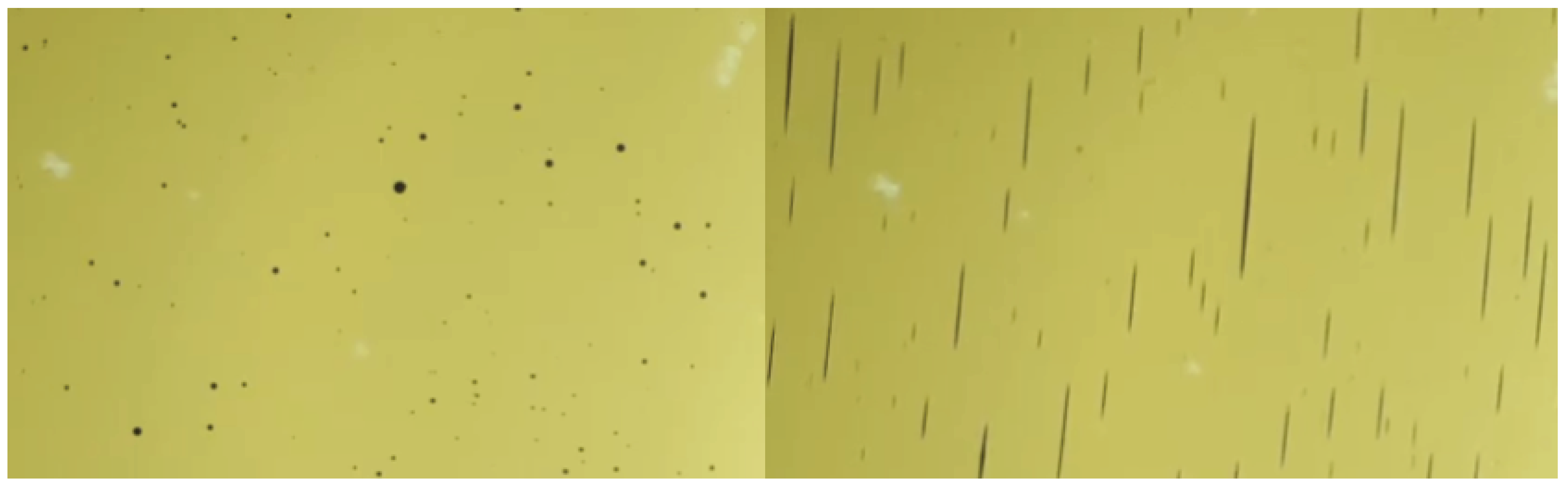
Figure 2.
a-d) Creation of the ferrolens. e) Experimental Setup: Ferrocell with light controls and camera above.
Figure 2.
a-d) Creation of the ferrolens. e) Experimental Setup: Ferrocell with light controls and camera above.
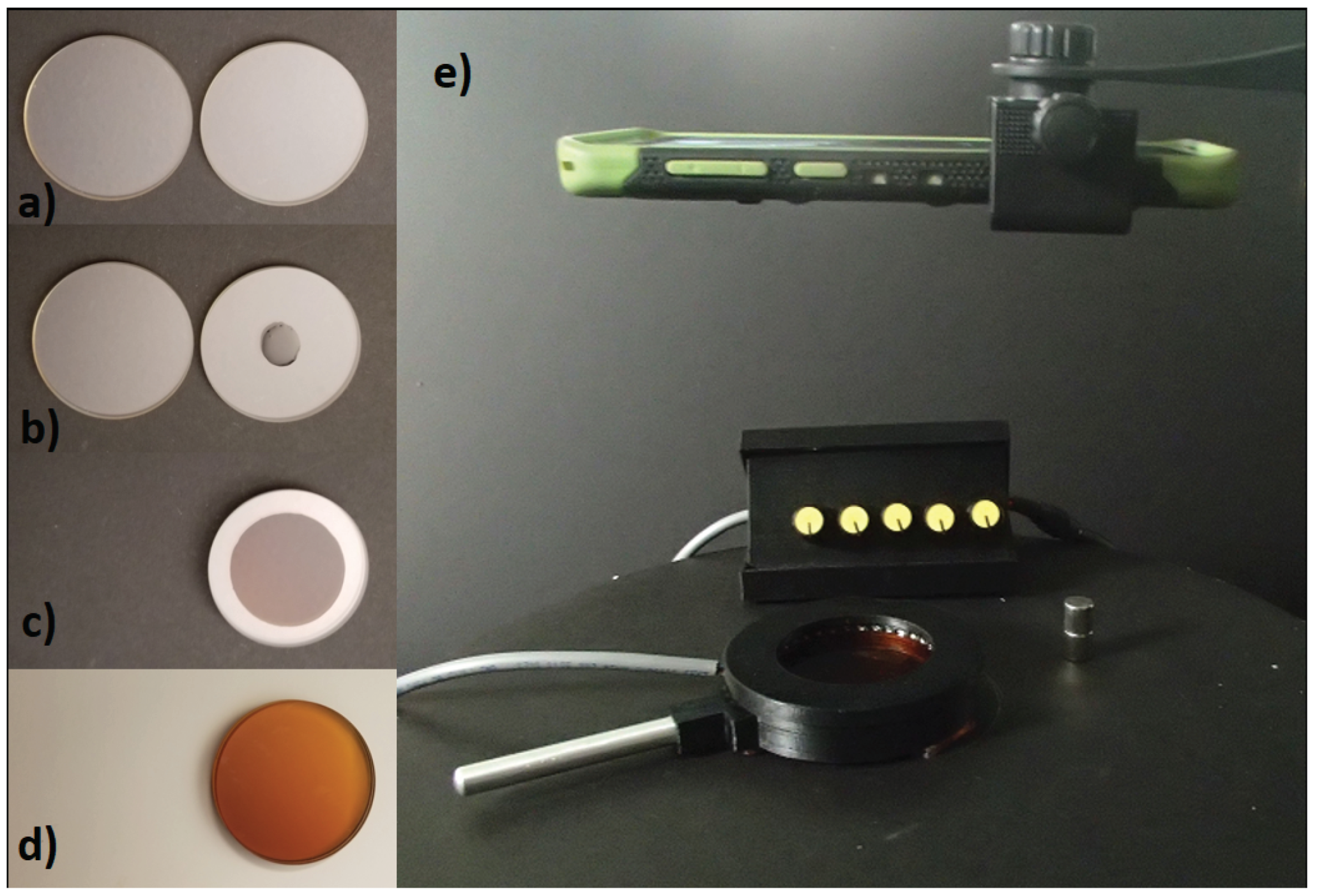
Figure 3.
Flow of control of the software developed to generate the Ferrocell images.
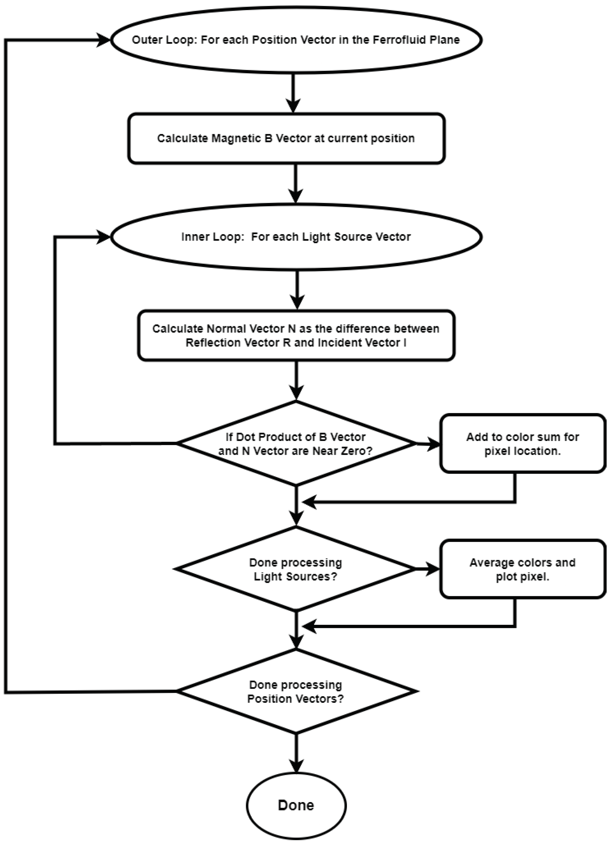
Figure 4.
Left: Cylinder magnet (d = 20mm, h = 25mm) under a 10cm diameter ferrolens. Polar view. A single white LED light source is used to illuminate the lens. Middle: Simulation of experimental setup. Right: Experiment and simulation merged together. Magnet highlighted.
Figure 4.
Left: Cylinder magnet (d = 20mm, h = 25mm) under a 10cm diameter ferrolens. Polar view. A single white LED light source is used to illuminate the lens. Middle: Simulation of experimental setup. Right: Experiment and simulation merged together. Magnet highlighted.
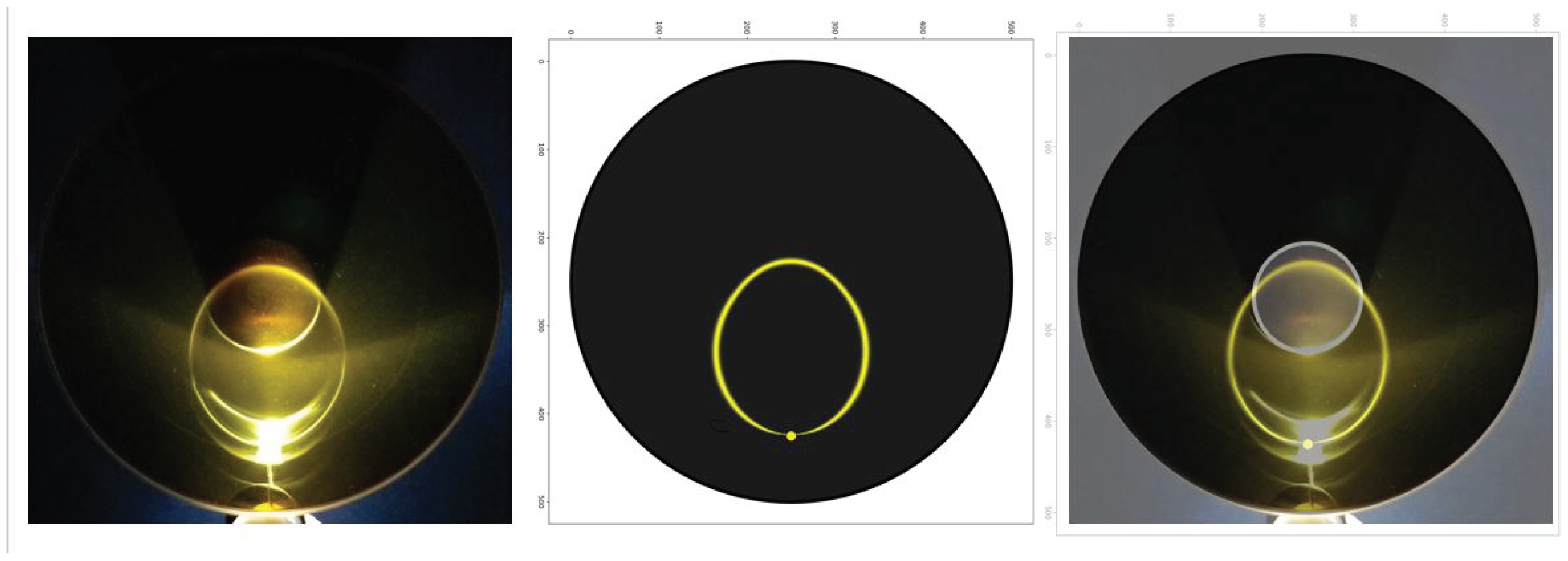
Figure 5.
Left: Experimental setup. Cylinder magnet (d = h = 10mm). Polar view. Ferrocell (d = 5cm), 36 lights. Right: Simulation of experimental setup. The magnet is highlighted in grey.
Figure 5.
Left: Experimental setup. Cylinder magnet (d = h = 10mm). Polar view. Ferrocell (d = 5cm), 36 lights. Right: Simulation of experimental setup. The magnet is highlighted in grey.
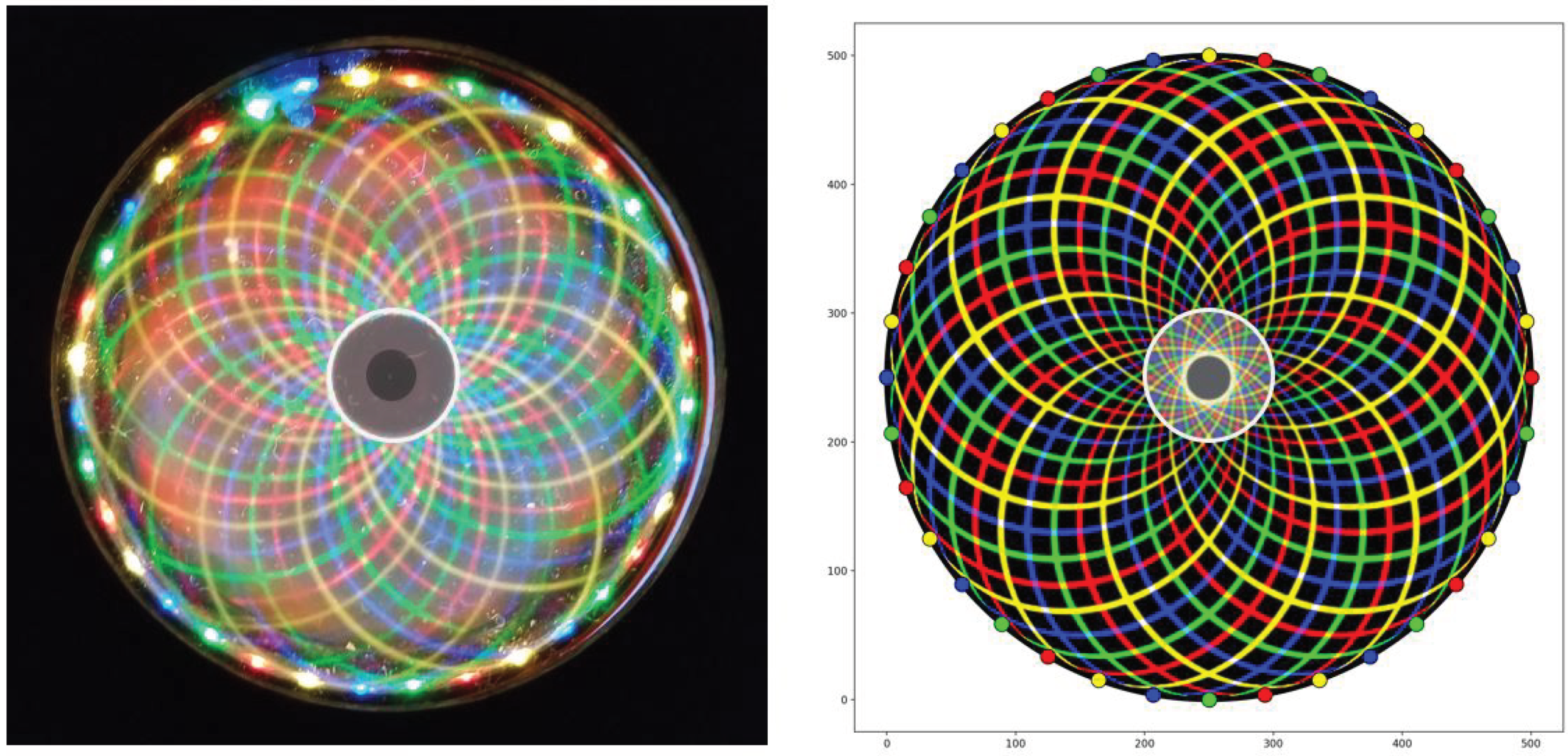
Figure 6.
Left: Experimental setup. Cube magnet (l = 2" w = 2" h = 1"), dipole view, 10cm ferrolens, 36 lights. Right: Simulation of experimental setup on left.
Figure 6.
Left: Experimental setup. Cube magnet (l = 2" w = 2" h = 1"), dipole view, 10cm ferrolens, 36 lights. Right: Simulation of experimental setup on left.
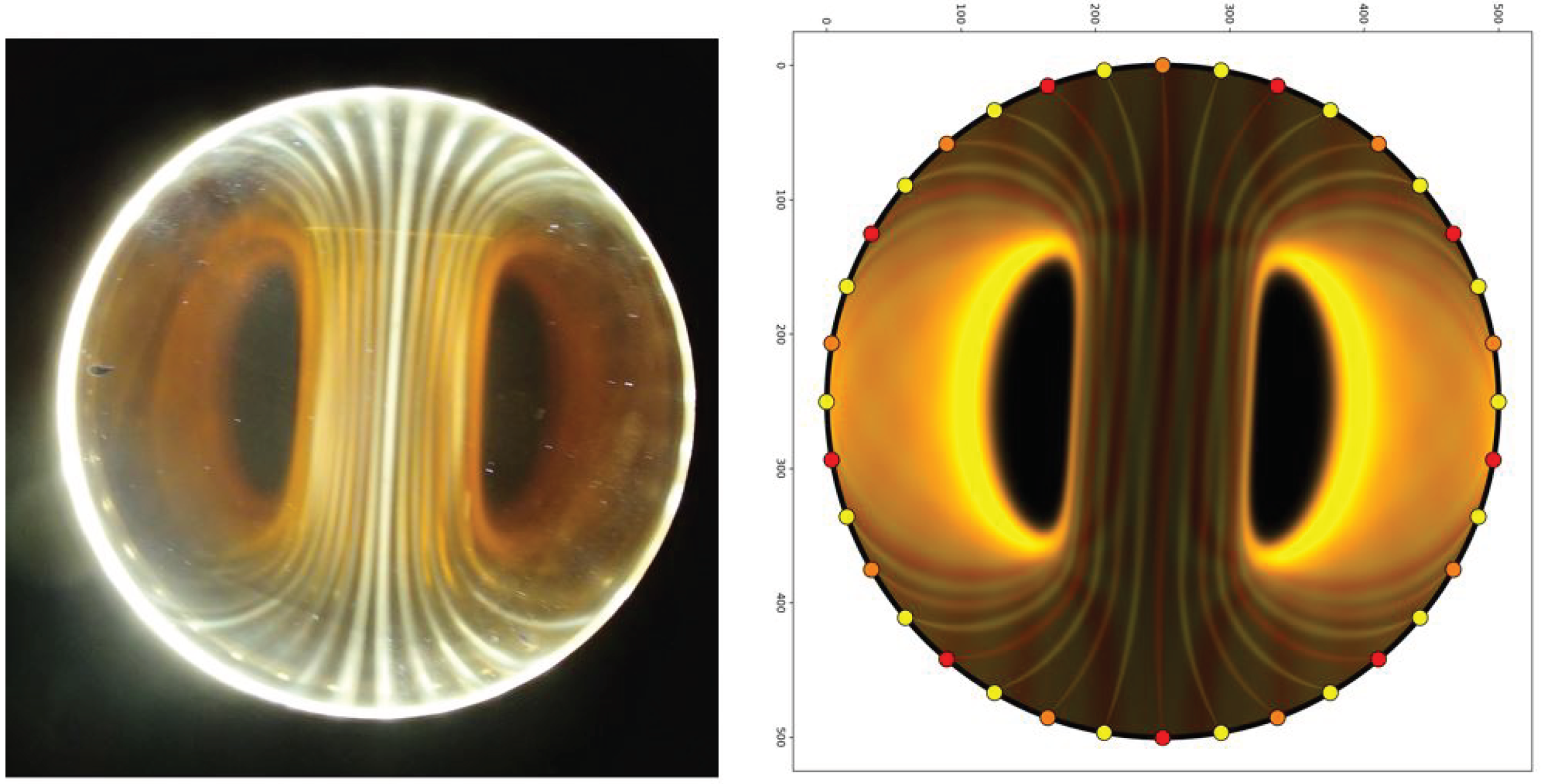
Figure 7.
Left: Experimental setup. Two magnets (d = h = 10mm). Side by side dipole view. Opposing poles, 5cm ferrocell, 36 lights. Right: Simulation of experimental setup.
Figure 7.
Left: Experimental setup. Two magnets (d = h = 10mm). Side by side dipole view. Opposing poles, 5cm ferrocell, 36 lights. Right: Simulation of experimental setup.
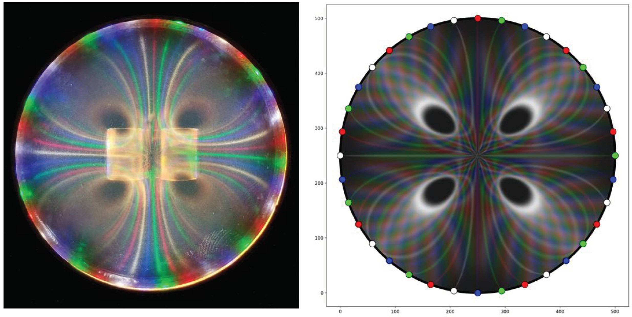
Figure 8.
Left: Central region of ferrocell with magnet hidden and top glass removed. Right: Central region of simulation.
Figure 8.
Left: Central region of ferrocell with magnet hidden and top glass removed. Right: Central region of simulation.
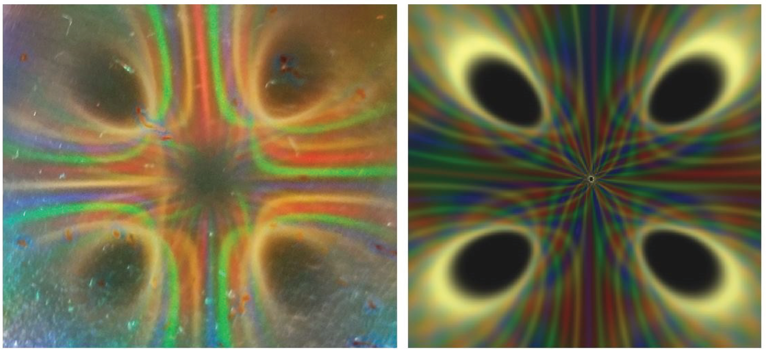
Figure 9.
Left: Ferrocell close up to show colour mixing when lines cross. Right: Simulation showing similar colour mixing at the intersections of the crossing lines.
Figure 9.
Left: Ferrocell close up to show colour mixing when lines cross. Right: Simulation showing similar colour mixing at the intersections of the crossing lines.
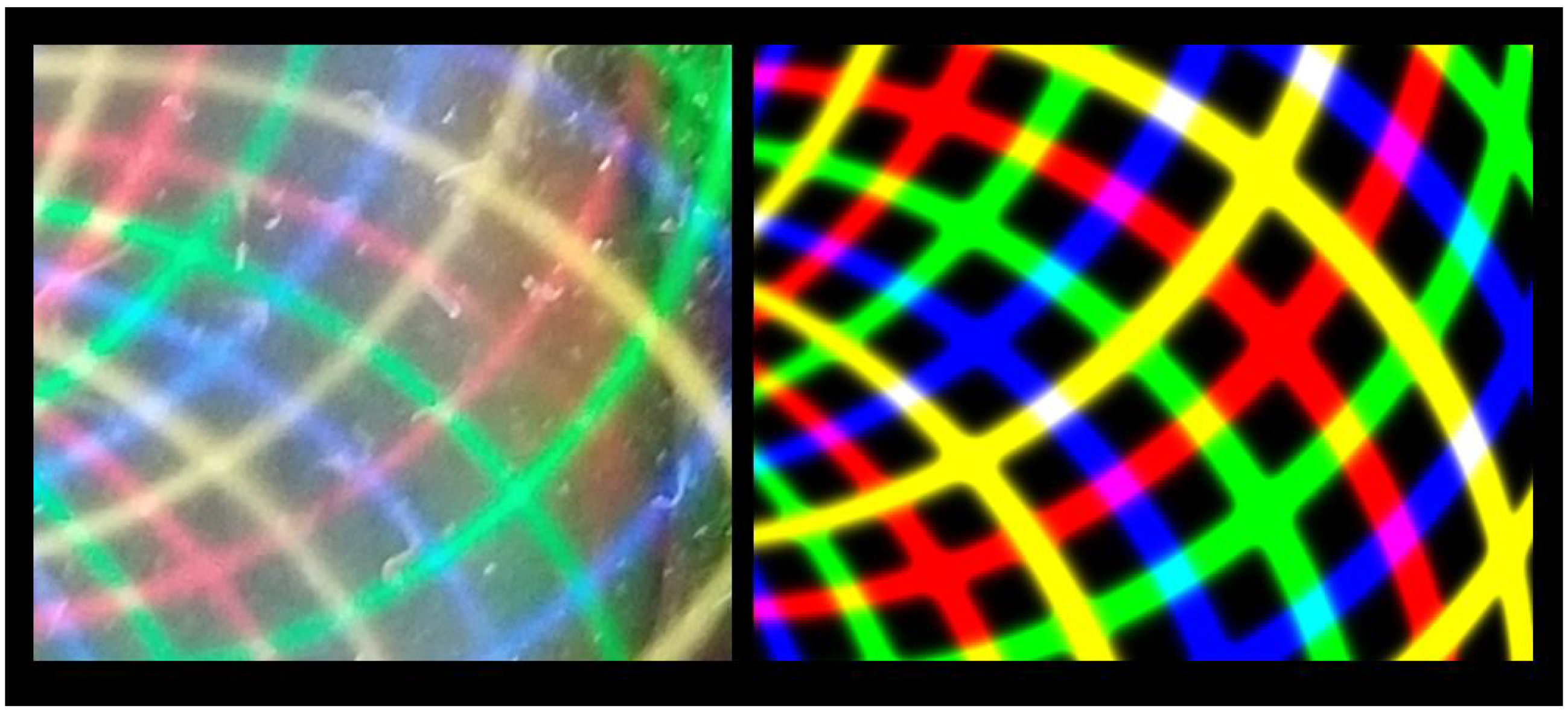
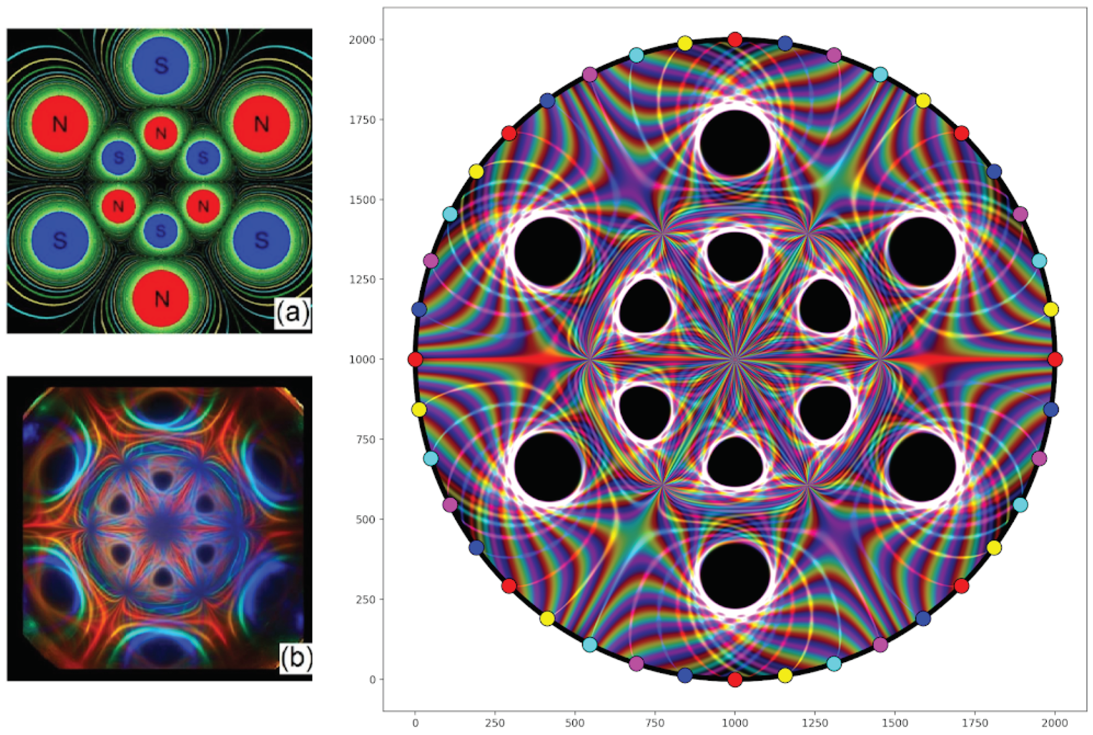
Figure 10.
Upper left: 12 Magnet configuration with associated isopotentials. Lower left: Ferrocell image of 12 magnet configuration. Right: Simulation of 12 magnet configuration.
Figure 10.
Upper left: 12 Magnet configuration with associated isopotentials. Lower left: Ferrocell image of 12 magnet configuration. Right: Simulation of 12 magnet configuration.
Disclaimer/Publisher’s Note: The statements, opinions and data contained in all publications are solely those of the individual author(s) and contributor(s) and not of MDPI and/or the editor(s). MDPI and/or the editor(s) disclaim responsibility for any injury to people or property resulting from any ideas, methods, instructions or products referred to in the content. |
© 2024 by the authors. Licensee MDPI, Basel, Switzerland. This article is an open access article distributed under the terms and conditions of the Creative Commons Attribution (CC BY) license (http://creativecommons.org/licenses/by/4.0/).
Copyright: This open access article is published under a Creative Commons CC BY 4.0 license, which permit the free download, distribution, and reuse, provided that the author and preprint are cited in any reuse.


