

Submitted:
07 February 2024
Posted:
08 February 2024
You are already at the latest version
Abstract
The spread of high-performance personal computers, frequently equipped with powerful Graphic Processing Units (GPU), raised the interest on a set of techniques able to extract models of electromagnetic phenomena (and devices) directly from available examples of the desired behavior. Such approaches are collectively referred to as Machine Learning (ML). A typical representative ML approach is the so called “Neural Network” (NN). Using such data-driven models allows evaluating the output in a much shorter time when a theoretical model is available, or allows predicting the behavior of the systems and devices when no theoretical model is available. With reference to a simple yet representative benchmark electromagnetic problem, some of the possibilities and the pitfalls of the use of NN for the interpretation of measurements (inverse problem) or to obtain the required measurements (optimal design problem) are discussed. The investigated aspects include the choice of the NN model; the generation of the dataset(s); the selection of hyperparameters (hidden layers, training paradigm). Finally, the capabilities in the handling of ill-posed problems are critically revised.
Keywords:
Machine Learning
; Magnetic Field Analysis
; Optimal Design
; Inverse Problems.
1. Introduction
Computerized analysis is frequently used to recover field sources or device structure from measurements using numerical computations [1,2]. This process implies the repeated resolution of an electromagnetic problem, under different trial values of inputs (either sources or system parameters). The presence of measurement noise, the consideration of manufacturing and assembly tolerances, the inclusion of ferromagnetic materials or the consideration of complex, three-dimensional geometries add relevant computational efforts to the process. Several measures have been proposed to simplify or speed-up the analysis, basically trading off accuracy in the evaluation of the distance of trial data from the actual measurements with promptness.
Alternatively, Machine Learning (ML) and Deep Learning (DL) models can be used for a straightforward resolution of inverse problems or optimal design ones, trying to train NN to build an (approximated) relationship between the desired output (e.g. sensors reading) and the trial values of the degrees of freedom (e.g. radii or currents of coils, when considering magnets) starting from available examples of the desired output [3,4,5,6,7]. Examples can be obtained by solving a reduced set of instances for the computationally demanding problem, or even be extracted for experimental data.
Note that the construction of an approximate model from available experimental data could reveal the sole possibility in cases where a theoretical problem formulation is not available. This could happen either when a model based on the laws of physics is not available or too complex to be reduced to a set of equations manageable in the due course of an iterative process.
In addition, the resulting problem, either the inverse one or the design one, shows an ill posed nature, being prone to multiple solutions [8,9]. This aspect has been counteracted in many ways, and some precaution must be taken also when using data-driven models.
In previous works the authors proposed several ML models both for solving the direct [10,11,12,13,14] model and the inverse model [15,16,17], focusing the attention on the optimization through the use of the direct model, and highlighting the difficulty behind the inverse models.
Data-driven models can be obtained following different approaches [8,10], including the classical statistical regressions or the most modern Deep Neural Networks. Each approach presents advantages and drawbacks, which must be comparatively assessed. In addition, the hyper-parameters shaping the approach (e.g. the number of hidden neurons in the NN case) must be carefully chosen to obtain the best balance between promptness and accuracy. This work presents a detailed analysis of the learning process for a set of NN models of a benchmark inverse problem. The data used to train the model are generated by FEM or analytical formulations.
The main aspects investigated in this work include:
- Training and testing ML approaches to solve direct and indirect electromagnetic problems;
- Selection of the ML model;
- Selection of the model hyper—parameters;
- Dataset generation;
- Regularization approaches;
- How machine learning treats ill posed inverse problems.
In the following, with reference to a simple yet representative benchmark problem, we will compare the standard Shallow Neural Networks (SNN) [18,19] with a more recent model, namely Convolutional Neural Networks (CNN) [20,21]. For the sake of comparison, also a support vector machine, as an example of regression model, will be introduced.
2. The Benchmark Problem
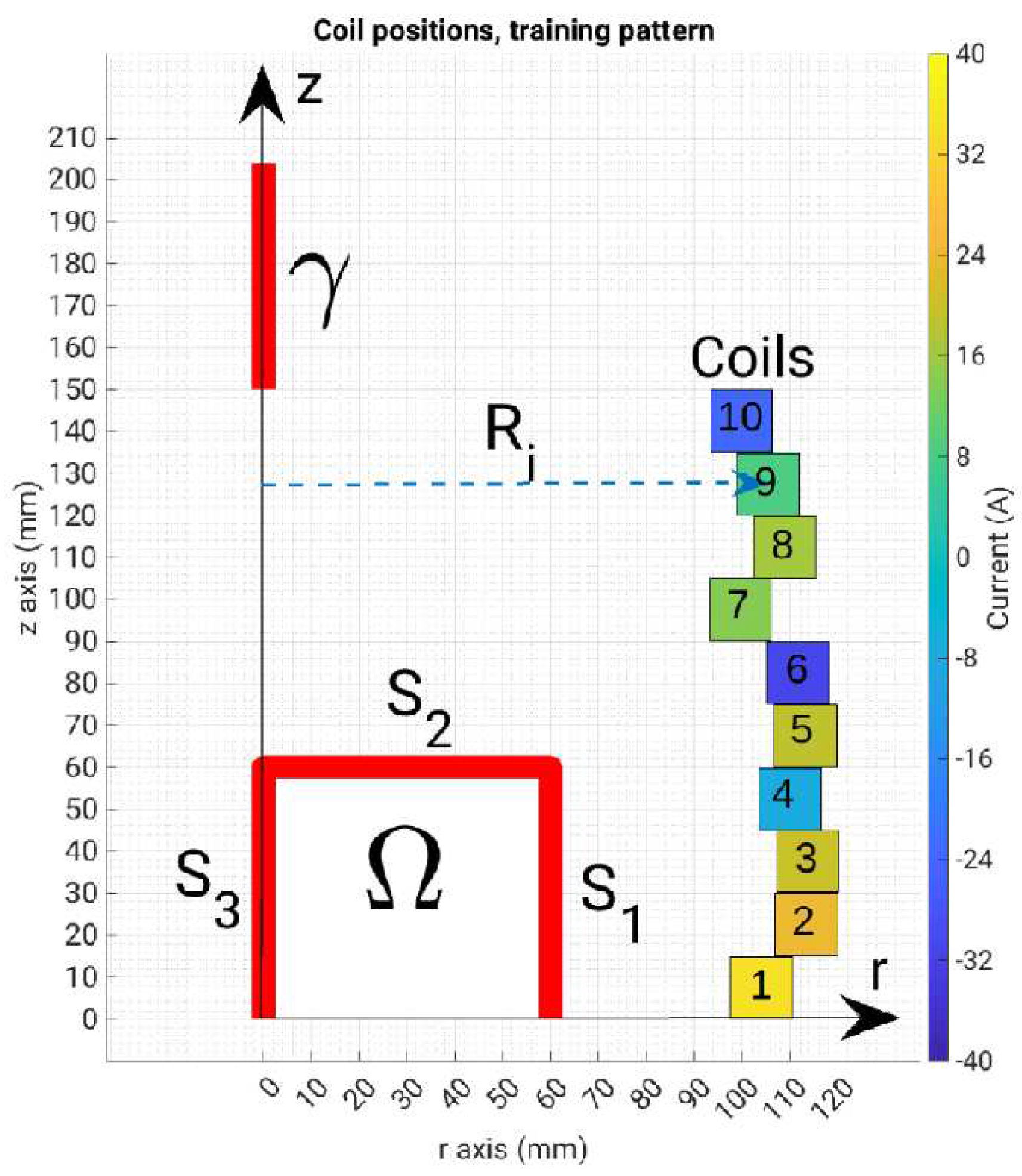
To compare different approaches, we adopt here the benchmark problem TEAM 35 [22]. A multi-turn air-cored coil is considered. The coil is composed of nt=20 independent turns. The width of each turn is w = 15 mm and the height is h = 10 mm. Hollow turns are assumed to allow for water circulation. In the following we will assume symmetric currents distribution among the uppermost 10 coils and the lowermost ones. Consequently, only half of the model is needed to compute the field (see Figure 1a). For evaluating the field, a two-dimensional controlled region is considered, (delimited by curves S1, … S3 in Figure 1a). The two components Br and Bz along axes r and z of the flux density field B are sampled on a grid evenly spaced in a square region with a side length of 60 mm, which is denoted as the Region Of Interest (ROI). Underlying sensors could be, e.g., Hall Probes.
To train the shallow neural network and the support vector regressor, we firstly consider a grid of np=10×10 field points, taking the values along the boundaries S1, … S3 and the line γ, while for the training of the convolutional neural network we consider a grid of np=20×20 field points, taking all the internal values of the square region of interest.
The magnetic analysis is based on the Finite Element (FE) method. An example of field map is shown in Figure 1b.
In the TEAM 35 version considered here, the aim of the inverse problem is to identify the radii and the currents in the coils to generate a prescribed flux density map B(r,z). In the original formulation, the map is uniform, with , within a region adjacent to the symmetry plane z=0 (lines S1, S2 and S3 in Figure 1), and with an amplitude as small as possible along an external segment of the symmetry axis (line γ in Figure 1). To evaluate the field uniformity in the inner ROI, the magnitude of B is “measured” in Np = 30 field points, evenly spaced on the boundary of the ROI. On the other hand, in order to guarantee the minimum field amplitude on γ, the field is “measured” on Nk = 10 points along γ. In particular, the set of measurements includes 60 real values, which correspond to 10 Br and 10 Bz measurements evenly spaced along lines S1 and S2 respectively, 10 Bz values measured along line S3, and 10 Bz values along line γ. In this paper, we maintain a similar formulation of the inverse problem, where we aim to identify the radii and the currents correspondent to randomly generated flux density measured in the measurement’s points.
Figure 2 shows the main characteristics of the variables involved in the problem. Note that when radii of all coils are known, the relationship between currents and flux density values is linear. The matrix mapping the current in each coil onto each single measurement is known as Lead Field Matrix (LFM). On the other hand, when the radii are among the degrees of freedom, the inverse problem gets non-linear, and the LFM must be, in principle, be re-assembled for each trial configuration. One of the advantages of the ML approaches is that the reassembly of the LFM is not required, as the NN directly extracts from data the relationship between field values (measurements) and the degrees of freedom (radii and currents).
More details on the benchmark problem geometry can be found in [10].
3. Considered Machine Learning Models
The machine learning models analyzed in this work will be used in different modalities:
- -
- a “Direct Problem” (DP), where examples of the radii/currents set and of the corresponding flux density values are used to create a model able to generate the target field map, hence replicating the LFM from the radii. The direct model is then used within traditional optimization or inverse problem resolution algorithms;
- -
- a first class of “Inverse Problem” (IP#1), where measurements (inputs) and currents (outputs) are used to create a model of the underlying linear map. In this case, radii are assumed known, and the linear model is related to the (pseudo-)inverse of the LFM.
- -
- a second class of “Inverse Problem” (IP#2), where the currents are known and provided as input together with the measurements, while the outputs are the radii;
- -
- finally, a third class (IP#3), where both currents and radii (the outputs) must be recovered from field measurements, which are the only inputs in this case.
Figure 3 shows the input and output of each defined problem. As anticipated, different ML approaches are available to create data-driven behavioral models. In this study, we have considered the following ones:
- Shallow Neural Networks (SNN) [18,19]: this is the standard approach: an artificial neural network with a single hidden layer with logistic activation functions. In the DP, Ni input neurons (corresponding to the radii), Nh hidden neurons and No output neurons (the elements of the LFM) are trained to provide the output. While Ni=10, the LFM will be represented by a reduced number of real numbers, corresponding to the main components in a PCA analysis based on the correlation analysis of the measurements. The full matrix is then recovered by exploiting the components identified in the PCA. In the inverse problems IP#1, IP#2 and IP#3, the SNN is used a straightforward solver, and the meaning of output neurons depends on the type of considered problem. This point will be further discussed below.
- The number Nh of hidden neurons is varied to assess model capabilities. The different SNN’s are trained using Levenberg-Marquardt Bayesian Regularization approach [23], which minimizes the weights together with the discrepancy on the data. Early topping is performed by means of worsen performance on a validartion set.
- Convolutional Networks (CNN) [20,21]. This class of NN will be considered for IP#3 only. A higher number of hidden layers is present here, and the network can be named “deep”. The inner layers are classified as “convolutional” and “pooling”, with different associated actions on the data. The activation functions are in this scheme the “ReLU” functions. This model has an intrinsic capability of building a reduced order inner model, which can be exploited to cope with the highly correlated nature of the input, represented by the flux density map in the ROI. The ADAM algorithm is used to train the CNN.
- In order to compare ML with more traditional statistical regression approaches, we have also considered Support-Vector Regression (SVR) [24,25] for the inverse problems. SVR training algorithm builds a linear model in a higher dimensional space exploiting the so called “kernel trick” by minimizing a quadratic objective function which is a combination of the Euclidean norm of the weights of the linear model and the sum of the so called slack variables, which represent a threshold of the maximum absolute deviation between the predicted and target values. The LIBSVM implementation of the SVR was employed
The hyper-parameters of the SNN and SVR models where selected using an exhaustive K-Fold Grid Search Cross Validation approach, using K=10 and a defining adequate ranges for the optimized hyper-parameters. The CNN architecture was selected using a trial and error heuristic approach, which is common for complex deep learning models.
Figure 4.
Representation of a random geometry, coils numbering and ROI.
4. Results
To assess the different models, 26000 examples have been generated using a FEM solver to compute the flux density in the measurement points. Examples have been arranged according to radii values, to identify different subsets with the same LFM, and divided into Training and Test sets, according to the 70/30 rule.
4.1. Direct Problem
In a first study we trained different SNN on the DP. The metric adopted here to compare the accuracy of the different predicted currents or radii is the Normalized Mean Absolute Error% (NMAE%).
NMAE% is an alternative metric that overcomes the limitations of more classical Mean Absolute Percentage Error in situations involving data that can be negative or close to zero. NMAE normalizes the error by dividing it by the range of the actual values, providing a more balanced measure of accuracy.
Figure 5a shows that the training of a SNN with 36 hidden neurons for the direct problem required 10 hours of computation in a 12 cores processor, while the convergence was obtained after 4 hours. The similar trend of the training and validation errors suggests that no the SNN is not overfitting. Figure 5b shows a test set pattern prediction, with respect to the target value, indicating that the prediction is qualitatively good. The NMAE% for the test set of the direct problem was 0.15%, indicating that the direct problem can be solved with good accuracy.
4.2. Inverse Problem #1
We then solved the inverse problem of type IP#1 by computing the Truncated-Pseudo-Inverse (TSVD) of either the SNN LFM and of the actual LFM, computed using FEM. Just 8 singular modes are used in this investigation. The currents obtained using the two inverse matrices are used to compute the flux density in the measurement points, and the results are compared with the original measurements.
Table I reports the test set NMAE% (normalized to 80A) of the 10 currents for the IP#1, solved by means of the SNN.
From Table 1 it can be observed that the NMAE% increases with the distance of the coil from the sampling curves S1..S3. The averaged NMAE% value is 1.66% In this case a SNN with 27 hidden neurons performed best. The average NMAE for SVR is 2.35%. SVR with Gaussian kernel has 3 real hyperparameters and searching them is difficult because a single training requires hours: better results were obtained with SNN.
The flux density in the “measurement” points corresponding to the different approaches are reported in Figure 6. The scatter plots shown in Figure 7 shows that the problem of predicting the currents can be solved by the neural networks accurately, and the dispersion increases with the distance for them sampling curves.
4.3. Inverse Problem #2
Very similar results are obtained for the inverse problem IP#2, reported in Table 2, again showing an increase of NMAE% with the distance from the measurement region. The averaged value is 10.34% for the SNN and 14.1% for the SVR. In this case a SNN with 35 hidden neurons performed best.
Figure 8.
Regression plots of the predicted vs true radii for IP#2.
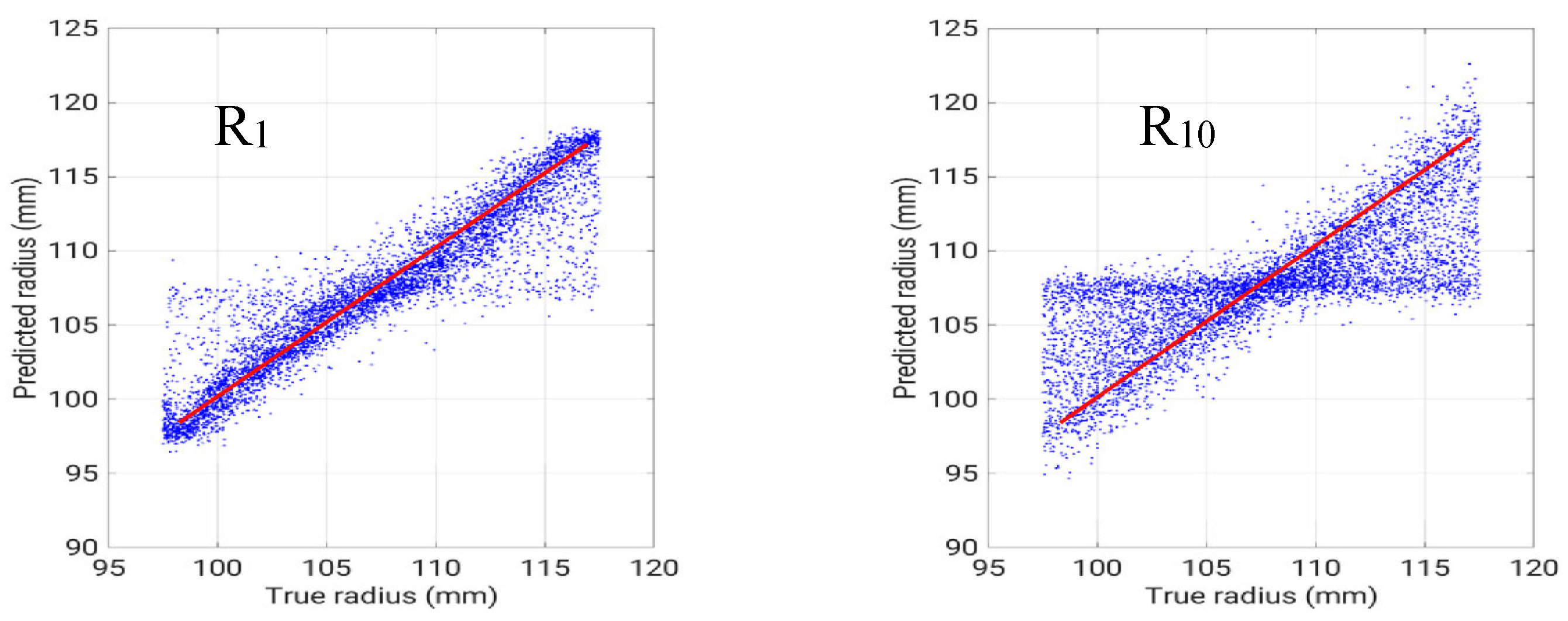
Figure 5 evidences that the problem of predicting the radii is more difficult, as expected.
4.4. Inverse Problem #3
Finally, for the inverse problem IP#3, the results for the currents confirmed the influence of the distance from the ROI, but with a slight recover in coils 9 and 10 when influence of γ line starts to be relevant. On the other hand, the radii show a completely different behavior (see Table 3).
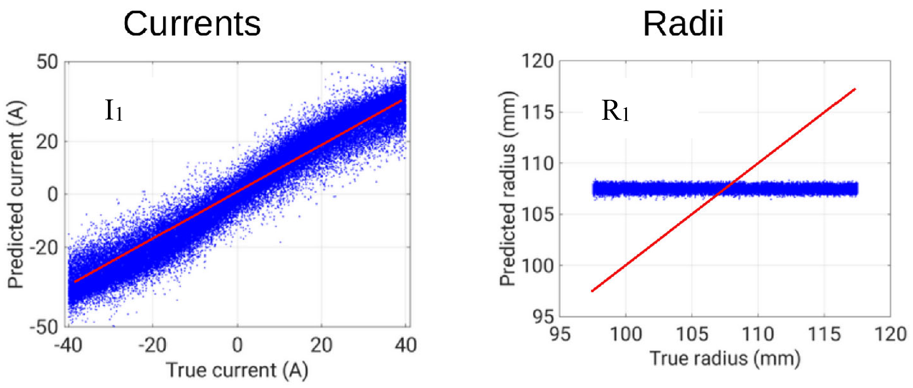
It is interesting to show the scatter plot of true vs. predicted radius for coil 1 for all the test cases (Figure 9). Basically, the SNN keeps the estimate of the radius equal to the average value, regardless of the actual value. This is due to the mutual role of current and radius in this problem. If considering the expression of the flux density on the axis due to a filamentary coil:
Figure 9.
catter plot of true and predicted values of current and radius of coil 1.
The above results for IP#3 where obtained with a SNN with 35 hidden neurons. We addressed the same problem using a CNN, but taking as inputs the whole Br and Bz images inside the ROI, considering a grid of 20x20.
The total number of inputs of the CNN is then the whole 2D ROI region 800 (as shown in Figure 10), compared to the 60 inputs along the ROI border used by the SNN, while the output of both methods are 10 radii values and 10 current values (as shown in Table 3). The architecture of the CNN is shown in Figure 11. The training of the CNN required 20 hours, while the training of the SNN and the SVR for the previous problems required 10 hours and 4 hours respectively. The results obtained with the CNN were almost identical to the results of the SNN, shown in Table 3 and Figure 6. Considering that the SNN adopts only the boundaries of the ROI as inputs and that the CNN considers the whole 2D domain, this result can be interpreted as a confirmation of the Dirichlet theorem for harmonic functions.
4.4. Inverse Problem #3: forward solution of inverted patterns
In order to assess the effectiveness of the radii and currents solutions obtained by the neural network for inverse problem IP#3, apart from calculating the errors in Table 3, we used these solutions as the input of the direct solver by means of a Finite Element Method, and compared the resulting field distribution with the input field distribution.
As a result, the NMAE% was 4.05%, where the normalization was performed against the mean absolute value of field inside the ROI.
Figure 12 shows three test examples of the true field values compared to the reconstructed field values using the FEM solution of the geometry obtained solving the inverse problem IP#3 with the SNN. From these results it can be stated that even if the error of the predicted radii is large, as can be observed in Figure 6 and Table 3, the combination of the predicted radii and currents represent a good source identification by means of the resulting field that is obtained applying the direct problem. The leverage of the SNN (and the CNN as well) consisting in applying the nonlinearities only to the current estimation appears to be an automatic way for regularizing the difficult inverse problem IP#3.
5. Discussion
The availability of different machine learning models for the prompt resolution of electromagnetic problems, as required in the inverse problems from electromagnetic measurements or in the optimization of electromagnetic devices, calls for a reciprocal comparison in terms of accuracy and promptness of the models, both in the training and operation phases. We proposed here a comparison among a few neural models on a well-known benchmark problem, considered here as an inverse problem.
The correlation among measurements from each sensor location (assessed on 26000 randomly distributed examples) shows that in the benchmark problem redundancy is present, although this redundancy is well managed by the machine learning and deep learning models, as shown by the results.
In the linear direct problem DP, the reconstruction of lead field matrix is straightforward, while for the three inverse problems, care must be taken in the choice of the regression algorithm. In the latter case IP#3, an interpolating model is achieved anyway, but generalization capability could be probably improved using “noisy” data. Neural network approach to linear inverse problem also requires careful choice of the learning strategy. As a remark, an accurately selected and trained SNN was shown to be a powerful model to solve the inverse problems, both linear and non-linear. The results obtained with the SNN and CNN for IP#3 show that a similar regularization was performed by two different models to approach the problem of infinite solutions of the inverse problem. Even if the radii and currents solutions were strongly regularized, they possessed both feasibility (they were inside the design bounds), and they turned to give good forward solutions when used as input of the direct problem. These results might be imputed more to the dataset itself than to the ML approach, confirming the results obtained in previous works [13]: the choice of the distribution of design parameters used to generate the training set is crucial for the performance of the ML approaches that are, of course, data driven.
Another quite remarkable result, which is new in the literature, is that the inversion of the electromagnetic problem gives the same results when using as input the field distribution in the boundary of the domain and the field distribution in the whole domain. Being the distribution inside the domain in theory dependent on the boundary conditions, that shall not be a complete surprise from a mathematical point of view, but it is not automatically expected that a neural network is able to incorporate this knowledge based on learning from data. The results obtained for the IP#3 solved by means of the SNN, which uses the boundary of the ROI, and the CNN, which uses the whole ROI; show that the SNN was able to acquire from the boundary values the same information that the CNN obtained from internal values. These results find confirmation in the recent development of the physics informed neural networks. For this reason, we are still working on the resolution of electromagnetic inverse and optimization problems with physics informed [26] and generative adversarial (game theory) neural networks [27].
Future work will be focused on the tuning of the NN for the inverse problem with a custom training loop using automatic differentiation. The idea is to back-propagate the error of the reconstructed field obtained by feeding the direct solver with the result of the NN.
Author Contributions
Conceptualization, A.F.; methodology, A.F. and M.T.; software, M.T.; formal analysis, A.F.; investigation, A.F. and M.T.; data curation, M.T.; writing—original draft preparation, A.F.; writing—review and editing, M.T. All authors have read and agreed to the published version of the manuscript.
Funding
This research received no external funding.
Institutional Review Board Statement
Not applicable
Informed Consent Statement
Not applicable
Acknowledgments
The authors wishes to thank Prof. Sami Barmada from Università di Pisa and Prof. Paolo di Barba and Prof. Maria Evelina Mognaschi for their continuing support and discussions.
Conflicts of Interest
The authors declare no conflicts of interest
References
- Mohammed, O.A.; Lowther, D.A.; Lean, M.H.; Alhalabi, B. On the creation of a generalized design optimization environment for electromagnetic devices. IEEE Transactions on Magnetics 2001, 37, 3562–3565. [Google Scholar] [CrossRef]
- Massa, A.; Salucci, M. On the design of complex EM devices and systems through the System-by-Design paradigm: A framework for dealing with the computational complexity. IEEE Transactions on Antennas and Propagation 2021, 70, 1328–1343. [Google Scholar] [CrossRef]
- Li, Y.; Lei, G.; Bramerdorfer, G.; Peng, S.; Sun, X.; Zhu, J. Machine learning for design optimization of electromagnetic devices: Recent developments and future directions. Applied Sciences 2021, 11, 1627. [Google Scholar] [CrossRef]
- Khan, A.; Lowther, D.A. Machine learning applied to the design and analysis of low frequency electromagnetic devices. In Proceedings of the IEEE 21st International Symposium on Electrical Apparatus & Technologies (SIELA 2020), Bourgas, Bulgaria, 03–06 June 2020; pp. 1–4. [Google Scholar] [CrossRef]
- Khan, A.; Ghorbanian, V.; Lowther, D. Deep learning for magnetic field estimation. IEEE Transactions on Magnetics 2019, 55, 1–4. [Google Scholar] [CrossRef]
- Khan, A.; Mohammadi, M.H.; Ghorbanian, V.; Lowther, D. Efficiency map prediction of motor drives using deep learning. IEEE Transactions on Magnetics 2020, 56, 1–4. [Google Scholar] [CrossRef]
- Rahman, M.M.; Khan, A.; Lowther, D.; Giannacopoulos, D. Evaluating magnetic fields using deep learning. COMPEL-The international journal for computation and mathematics in electrical and electronic engineering 2023, 42, 1113–1130. [Google Scholar] [CrossRef]
- Formisano, A. A comparison of different formulations for an inverse source magnetostatic problem. In Proceedings of the International Applied Computational Electromagnetics Society Symposium (ACES 2019), Miami, FL, USA, 14‐19 April 2019; pp. 1‐2, url: https://ieeexplore.ieee.org/document/8713032.
- Formisano, A.; Martone, R. Different regularization methods for an inverse magnetostatic problem. International Journal of Applied Electromagnetics and Mechanics 2019, 60, S49–S62. [Google Scholar] [CrossRef]
- Barmada, S.; Fontana, N.; Sani, L.; Thomopulos, D; Tucci, M. Deep learning and reduced models for fast optimization in electromagnetics. IEEE Transactions on Magnetics 2020, 56, 1‐4. [CrossRef]
- Barmada, S.; Tucci, M.; Sani, L.; Tozzo, C. Deep Neural Network Based Electro‐Mechanical Optimization of Electric Motors. IEEE Transactions on Magnetics 2022, 59, 8201204‐ 8201204. [CrossRef]
- Tucci, M.; Barmada, S.; Sani, L.; Thomopulos, D.; Fontana, N. Deep neural networks based surrogate model for topology optimization of electromagnetic devices. In Proceedings of the International Applied Computational Electromagnetics Society Symposium (ACES 2019), Miami, FL, USA, 14–19 April 2019; pp. 1–2, url: https://ieeexplore.ieee.org/document/8712975. [Google Scholar]
- M. Tucci, S. Barmada, A. Formisano and D. Thomopulos. A regularized procedure to generate a deep learning model for topology optimization of electromagnetic devices. Electronics, vol. 10, 2021. [CrossRef]
- Barmada, S.M; Fontana, N.; Formisano, A.; Thomopulos, D.; Tucci, M. A deep learning surrogate model for topology optimization. IEEE Transactions on Magnetics 2021, 57, 1–4. [Google Scholar] [CrossRef]
- Barmada, S.; Di Barba, P.; Formisano, A.; Mognaschi, M.E.; Tucci, M. Learning-Based Approaches to Current Identification from Magnetic Sensors. Sensors 2023, 23, 3832. [Google Scholar] [CrossRef]
- Barmada, S.; Formisano, A.; Thomopulos, D.; Tucci, M. Deep learning as a tool for inverse problems resolution: a case study. COMPEL-The international journal for computation and mathematics in electrical and electronic engineering 2022, 41, 2120–2133. [Google Scholar] [CrossRef]
- Barmada, S.; Barba, P.D.; Fontana, N.; Mognaschi, M.E.; Tucci, M. Electromagnetic Field Reconstruction and Source Identification Using Conditional Variational Autoencoder and CNN. IEEE Journal on Multiscale and Multiphysics Computational Techniques 2023, 8, 322–331. [Google Scholar] [CrossRef]
- Haykin, S. Neural networks and learning machines, 3rd ed.; Prentice Hall: New York, NY, USA, 2011; ISBN 13-978-8131763773. [Google Scholar]
- Aggarwal, C.C. Neural Networks and Deep Learning; Springer Nature Switzerland AG: Cham, Switzerland, 2018; ISBN 978-3-319-94463-0. [Google Scholar] [CrossRef]
- Goodfellow, I.; Bengio, Y.; Courville, A. Deep learning; MIT press: Cambridge, MA, USA, 2016; ISBN 13-9780262035613. [Google Scholar]
- Aggarwal, C.C. Neural Networks and Deep Learning; Springer Nature Switzerland AG: Cham, Switzerland, 2018; Convolutional Neural Networks, pp 315–371; ISBN 978-3-319-94463-0. [CrossRef]
- Alotto, P.; Di Barba, P.; Formisano, A.; Lozito, G.M.; Martone, R.; Mognaschi, M.E.; Repetto, M.; Salvini, A.; Savini, A. Synthesizing sources in magnetics: a benchmark problem 2021, COMPEL-The international journal for computation and mathematics in electrical and electronic engineering, 40, 1084-1103. [CrossRef]
- Foresee, F.D.; Hagan, M.T. Gauss-Newton approximation to Bayesian learning. In Proceedings of the International Joint Conference on Neural Networks (IJCNN 1997), Houston, TX, USA, 12–12 June 1997; pp. 1930–1935. [Google Scholar] [CrossRef]
- Cortes, C.; Vapnik, V. Support-vector networks. Mach Learn 1995, 20, 273–297. [Google Scholar] [CrossRef]
- Smola, A.J.; Schölkopf, B. A tutorial on support vector regression. Statistics and computing 2004, 14, 199–222. [Google Scholar] [CrossRef]
- Khan, A.; Lowther, D.A. Physics informed neural networks for electromagnetic analysis. IEEE Transactions on Magnetics 2022, 58, 1–4. [Google Scholar] [CrossRef]
- Creswell, A.; White, T.; Dumoulin, V.; Arulkumaran, K.; Sengupta, B.; Bharath, A.A. Generative adversarial networks: An overview. IEEE signal processing magazine 2018, 35, 53–65. [Google Scholar] [CrossRef]
Figure 1.
A sketch of the TEAM 35 benchmark problem: compute the magnetic field components along the red lines generated by a set of coils with radii R1, R2, …R10. (a): the problem geometry, (b): an example of field map.
Figure 1.
A sketch of the TEAM 35 benchmark problem: compute the magnetic field components along the red lines generated by a set of coils with radii R1, R2, …R10. (a): the problem geometry, (b): an example of field map.
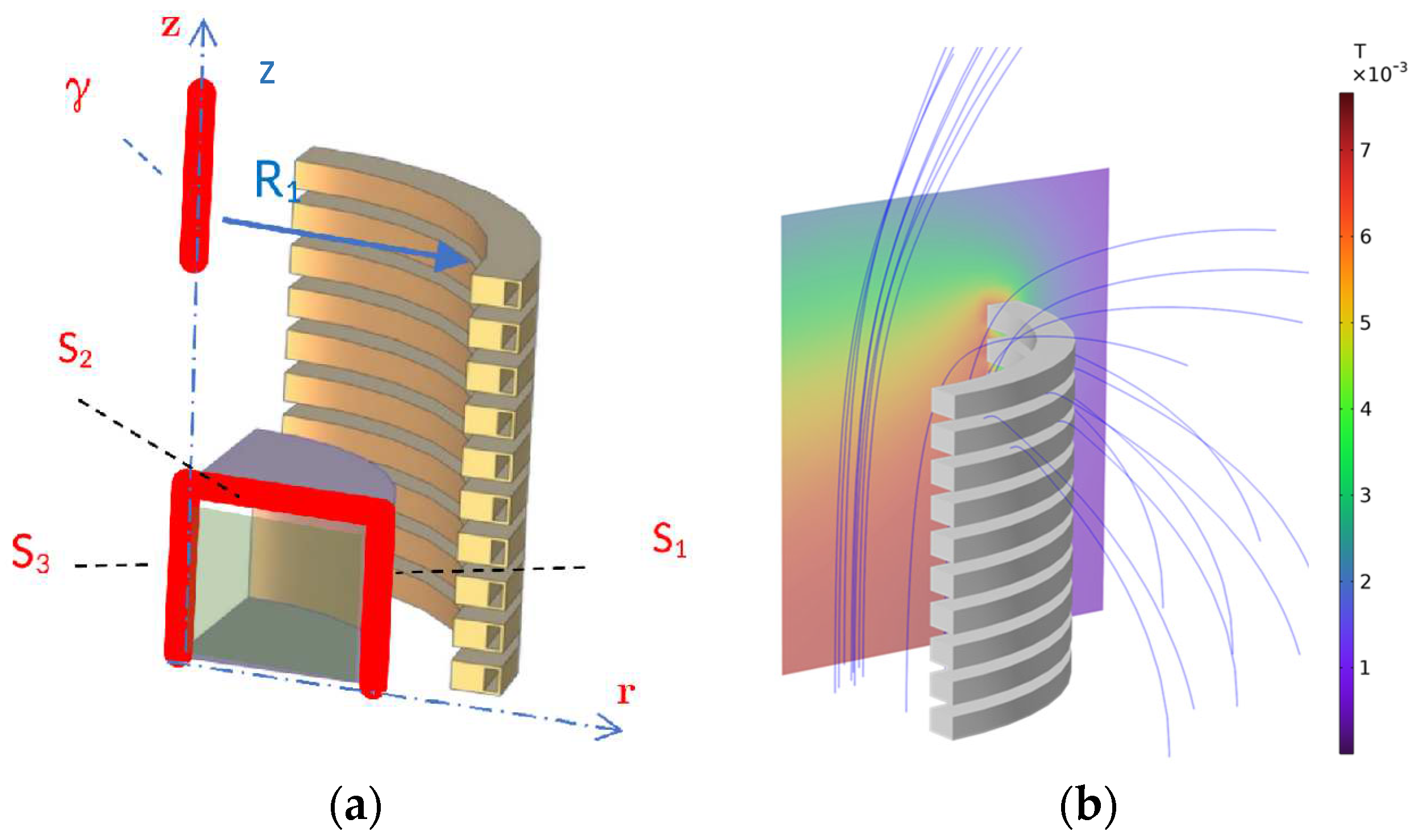
Figure 2.
Characteristics of the sources and of the measurements of the benchmark problem.
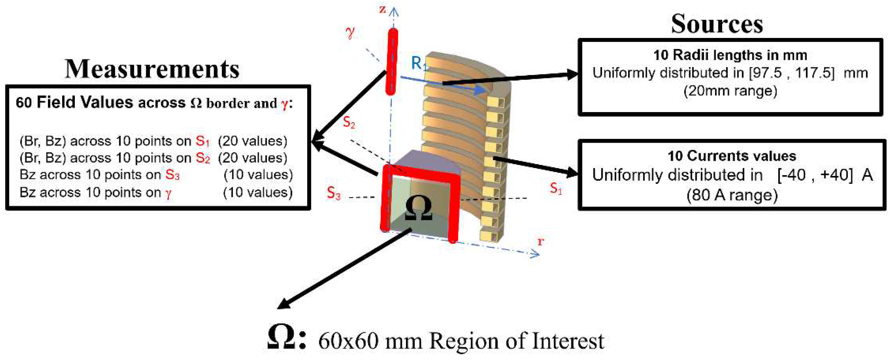
Figure 3.
Definition of the direct and inverse problems.
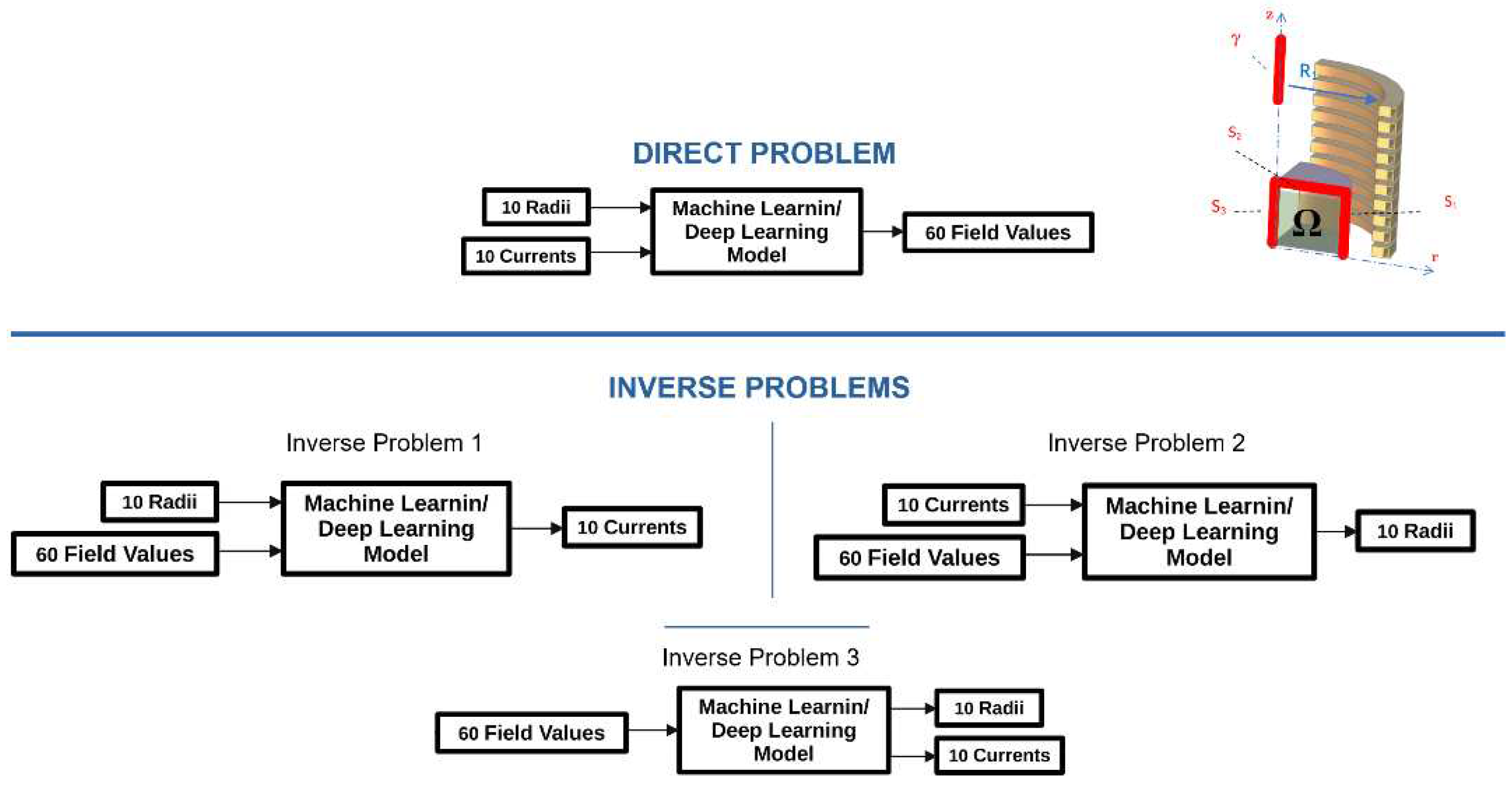
Figure 5.
Training error convergence a) and example of a test field pattern prediction b) of the direct problem solved by means of the SNN.
Figure 5.
Training error convergence a) and example of a test field pattern prediction b) of the direct problem solved by means of the SNN.
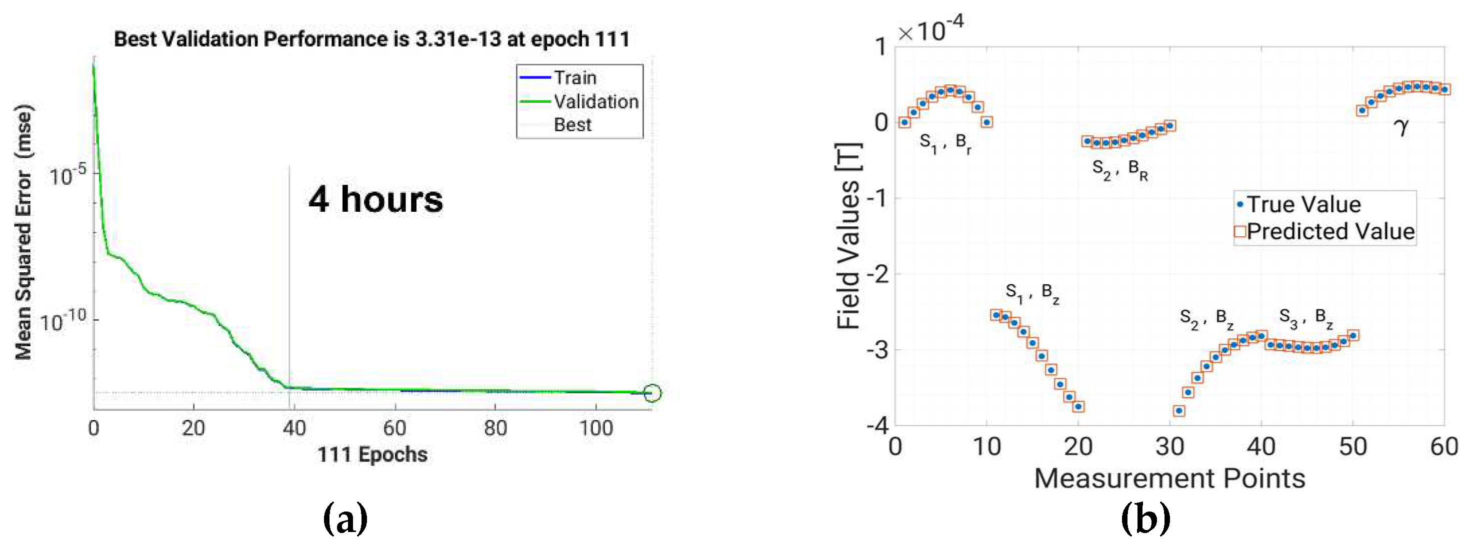
Figure 6.
Actual flux density values in the measurement points (blue curve), compared with the values obtained using currents identified using the tSVD of LFM as generated by FEM (red continuous line) or as generated by SNN (red crosses line).
Figure 6.
Actual flux density values in the measurement points (blue curve), compared with the values obtained using currents identified using the tSVD of LFM as generated by FEM (red continuous line) or as generated by SNN (red crosses line).
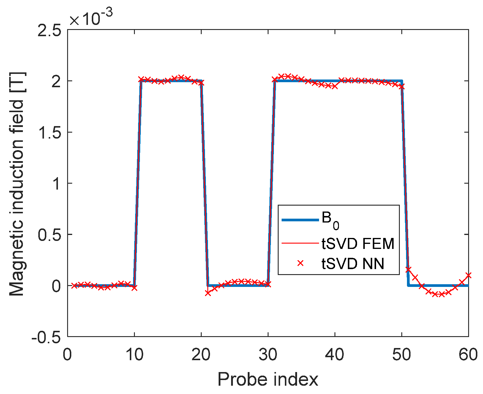
Figure 7.
Regression plots of the predicted vs true currents for IP#1.
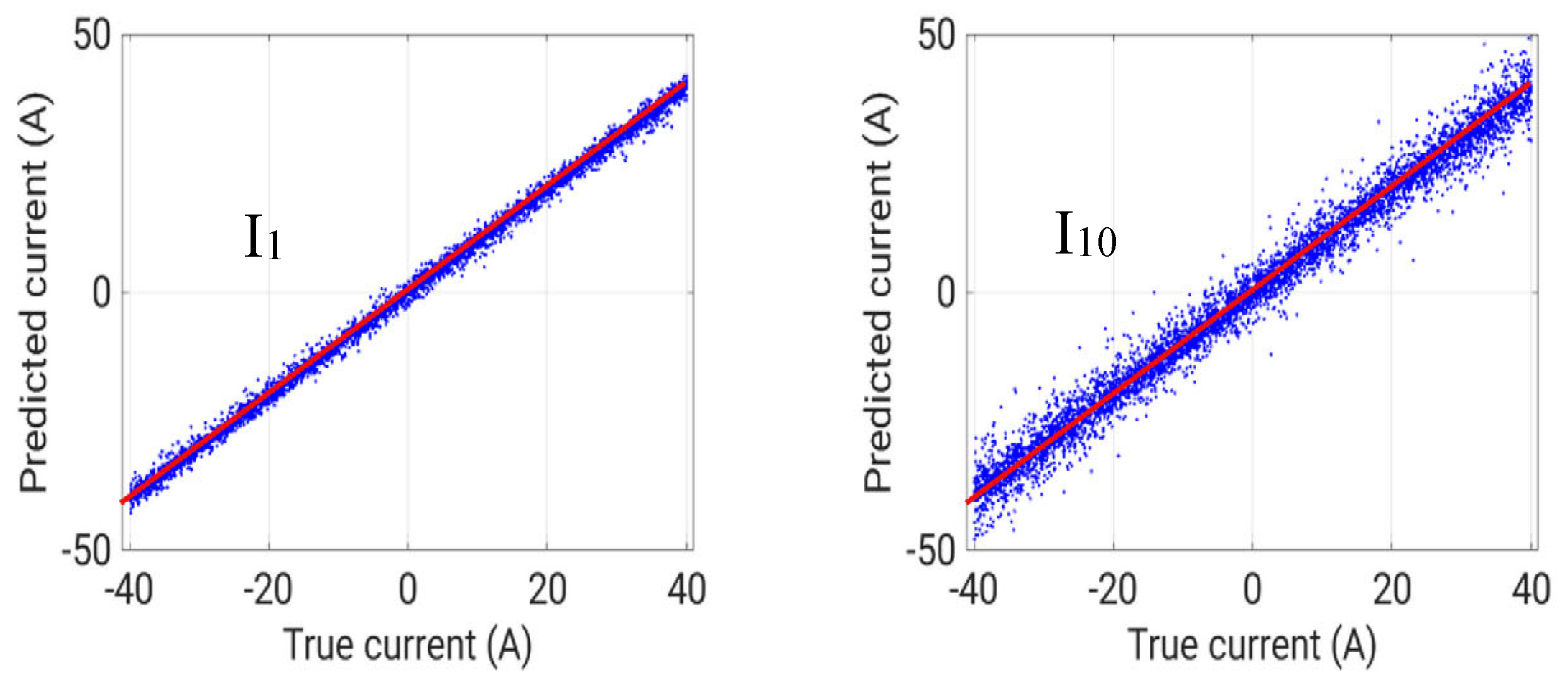
Figure 10.
Training pattern for the CNN, depicting the input images of the distribution of Br and Bz inside the region of interest.
Figure 10.
Training pattern for the CNN, depicting the input images of the distribution of Br and Bz inside the region of interest.
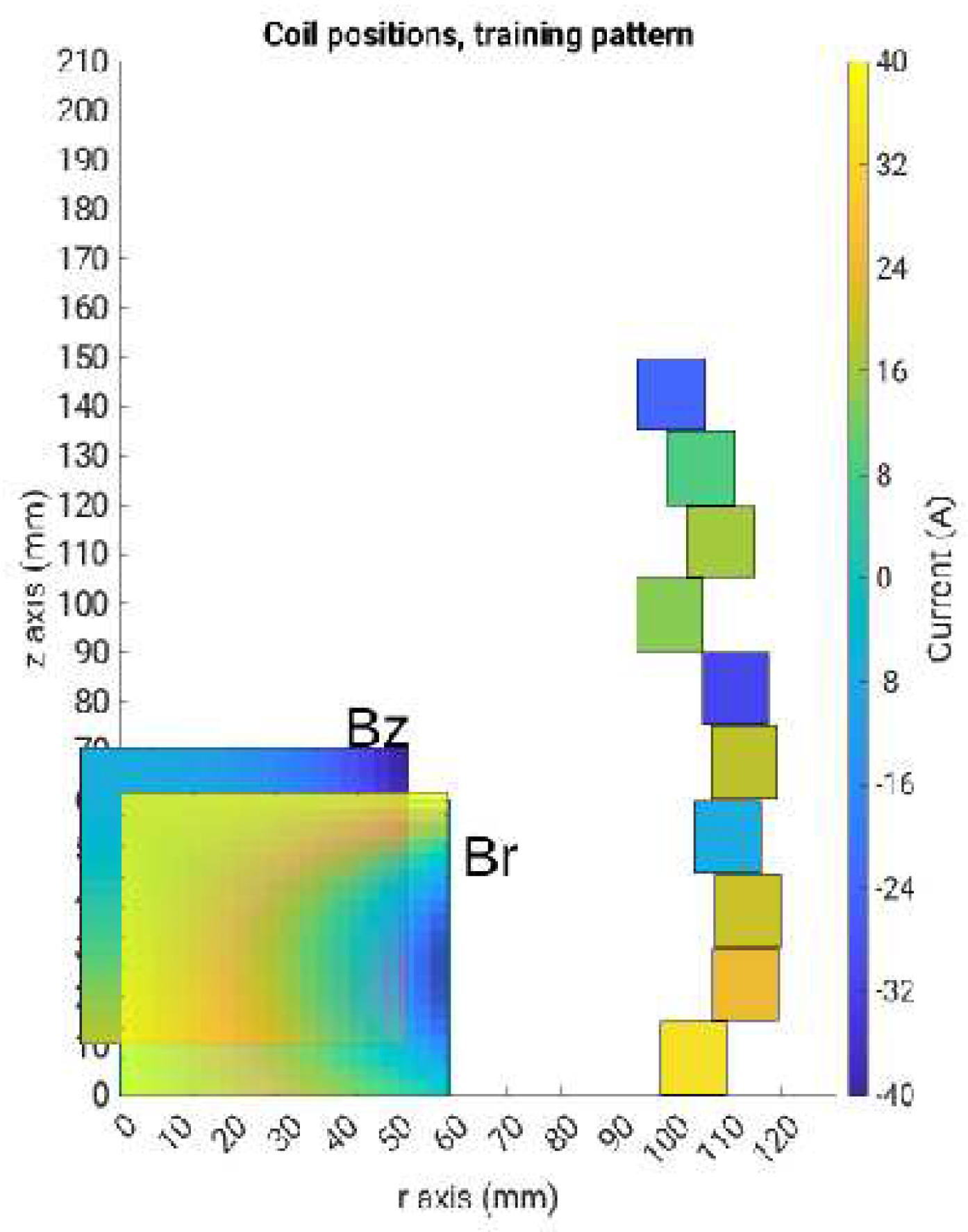
Figure 11.
Architecture of the Convolutional Neural Network for inverse problem #3.
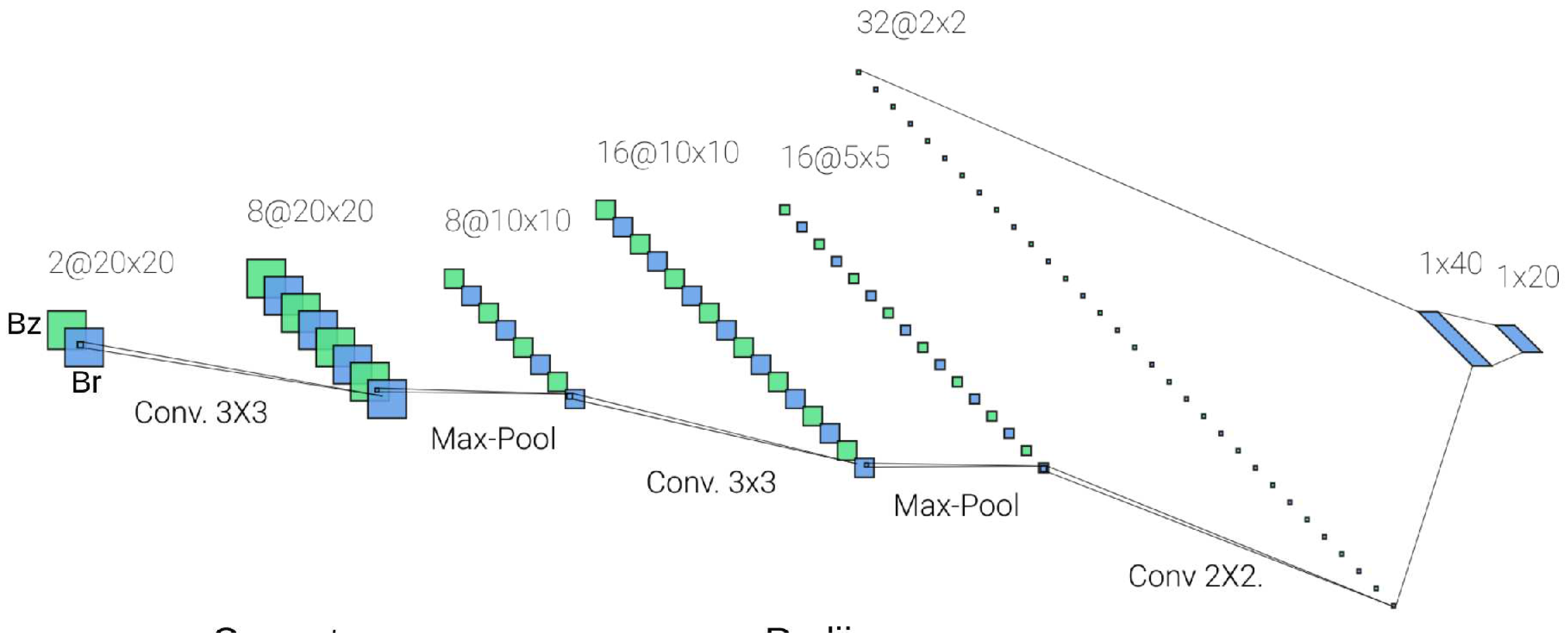
Figure 12.
Comparison between the reconstructed and true values of the field, after feeding the FEM direct solver with the neural network solutions of IP#3.
Figure 12.
Comparison between the reconstructed and true values of the field, after feeding the FEM direct solver with the neural network solutions of IP#3.


Table 1.
NMAE% for IP#1.
| I1 | I2 | I3 | I4 | I5 | I6 | I7 | I8 | I9 | I10 |
|---|---|---|---|---|---|---|---|---|---|
| 0.91% | 0.98% | 1.11% | 1.12% | 1.44% | 1.54% | 2.22% | 2.69% | 2.24% | 2.21% |
Table 2.
NMAE% for IP#2.
| R1 | R2 | R3 | R4 | R5 | R6 | R7 | R8 | R9 | R10 |
|---|---|---|---|---|---|---|---|---|---|
| 6.75% | 7.67% | 8.42% | 8.71% | 10.40% | 9.14% | 12.94% | 13.23% | 12.98% | 13.14% |
Table 3.
NMAE% for IP#3.
| I1 | I2 | I3 | I4 | I5 | I6 | I7 | I8 | I9 | I10 |
|---|---|---|---|---|---|---|---|---|---|
| 3.53% | 4.47% | 4.48% | 4.51% | 4.54% | 5.15% | 5.85% | 7.19% | 6.97% | 2.21% |
| R1 | R2 | R3 | R4 | R5 | R6 | R7 | R8 | R9 | R10 |
| 24.53% | 24.40% | 24.62% | 26.06% | 25.34% | 24.61% | 25.97% | 24.49% | 26.04% | 24.44% |
Disclaimer/Publisher’s Note: The statements, opinions and data contained in all publications are solely those of the individual author(s) and contributor(s) and not of MDPI and/or the editor(s). MDPI and/or the editor(s) disclaim responsibility for any injury to people or property resulting from any ideas, methods, instructions or products referred to in the content. |
© 2024 by the authors. Licensee MDPI, Basel, Switzerland. This article is an open access article distributed under the terms and conditions of the Creative Commons Attribution (CC BY) license (http://creativecommons.org/licenses/by/4.0/).
Copyright: This open access article is published under a Creative Commons CC BY 4.0 license, which permit the free download, distribution, and reuse, provided that the author and preprint are cited in any reuse.


