Optimizing EMG Classification through Metaheuristic Algorithms

1. Introduction

Classifying electromyographic signals (EMG) corresponding to movements is a fundamental task in biomedical engineering and has been widely studied in recent years. EMG signals are electrical records of muscle activity that contain valuable information about muscle contraction and relaxation patterns. Accurate classification of these signals is essential for various applications, such as EMG-controlled prosthetics, rehabilitation, and monitoring of muscle activity [1].

One recently used method to classify EMG signals is the multilayer perceptron (MLP). This artificial neural network architecture has proven effective in signal processing and pattern classification. MLP consists of several layers of interconnected neurons, each activated by a non-linear function. These layers include an input layer, one or more hidden layers, and an output layer. Although MLPs are suitable for classifying EMG signals, their performance is strongly affected by the choice of hyperparameters. Hyperparameters are configurable values that are not learned directly from the dataset but do define the behavior and performance of the model. Some examples of hyperparameters in the MLP context are [2,3,4]:

•

Number of neurons in hidden layers: This hyperparameter determines the generalization power of the model. Few neurons lead to underfitting, while too many lead to overfitting.

•

Learning rate: This factor determines how much the network weights are adjusted during the learning process. A high learning rate prevent the model from converging, while a low learning rate slow the training process.

•

Training Periods—Indicates the number of times the network weights were updated during training using the complete data set. An insufficient number of epochs leads to the undertraining of the model, while too many epochs lead to overtraining.

•

Training batch size: The number of training samples to use each time the weights are updated. The batch size affects the stability of the training process and the speed of convergence of the model.

Traditionally, hyperparameter selection has involved a trial-and-error process of exploring different combinations of values to determine the best performance. However, this approach is time-consuming and computationally intensive, especially with ample search space. Automated hyperparameter search methods have been developed to address this problem [5]. In this context, it is proposed to use particle swarm optimization (PSO) and gray wolf optimization (GWO) algorithms to select the hyperparameters of the MLP model automatically. These metaheuristic optimization algorithms effectively find the optimal solution in a given search space.

PSO and GWO work similarly, generating an initial set of possible solutions and iteratively updating them based on their performance. Each solution is a combination of MLP hyperparameters. The objective of these algorithms is to find the combination of hyperparameters that maximizes the performance of the MLP model in the classification of EMG signals [6].

The performed experiments show that hyperparameter optimization significantly improves the performance of MLP models in classifying EMG signals. The optimized MLP model achieved a classification accuracy of 93% in the validation phase, which is promising.

The current work is structured as follows: Section 2 provides a comprehensive literature review, offering insights into the proposed work. In Section 3, the methods and definitions essential for the development of the project are outlined. Section 4 presents the sequential steps to be followed in order to implement the proposed algorithm. The results and discoveries obtained are presented in Section 5. Section 6 presents the interpretation of the results from the perspective of previous studies and working hypotheses. Lastly, the areas covered by the scope of this work are presented in Section 7.

2. Related works

In signal processing, particularly electromyography, various approaches have been proposed to enhance the accuracy of pattern recognition models. In 2018, Purushothaman et al. [7] introduced an efficient pattern recognition scheme for controlling prosthetic hands using EMG signals. The study utilized eight EMG channels from eight able-bodied subjects to classify 15 finger movements, aiming for optimal performance with minimal features. The EMG signals were preprocessed using a dual-tree complex wavelet transform. Subsequently, several time-domain features were extracted, including zero crossing, slope sign change, mean absolute value, and waveform length. These features were chosen to capture relevant information from the EMG signals.

The results demonstrated that the naive Bayes classifier and ant colony optimization achieved an average precision of 88.89% in recognizing the 15 different finger movements using only 16 characteristics. This outcome highlights the effectiveness of the proposed approach in accurately classifying and controlling prosthetic hands based on EMG signals.

On the other hand, in 2019, Too et al. [8] proposed using Pbest-guide binary particle swarm optimization to select relevant features from EMG signals decomposed by discrete wavelet transform, managing to reduce more than 90% of features while maintaining average classification accuracy of 88%. Also, Sui et al. [9] proposed using the wavelet package to decompose the EMG signal and extract the energy and variance of the coefficients as feature vectors. They combined PSO with an enhanced support vector machine (SVM) to build a new model, achieving an average recognition rate of 90.66% and reducing training time by 0.042 seconds.

In 2020, Kan et al. [10] proposed an EMG pattern recognition method based on a recurrent neural network optimized by the PSO algorithm, obtaining a classification accuracy of 95.7%.

One year later, in 2021, Bittibssi et al. [11] implemented a recurrent neural network model based on long-term, short-term memory, Convolution Peephole LSTM, and Gated Recurrent Unit to predict movements from sEMG signals. Various techniques were evaluated and applied to six reference data sets, obtaining a prediction accuracy of almost 99.6%. In the same year, Li et al. [12] developed a scheme for classifying 11 moves using three feature selection methods and four classification methods. They found that the TrAdaBoost-based incremental SVM method requested the highest classification accuracy. The PSO method achieved a classification accuracy of 93%.

As well, Cao et al. [13] proposed an sEMG gesture recognition model that combines feature extraction, genetic algorithm, and support vector machine model with a new adaptive mutation particle swarm optimization algorithm to optimize SVM parameters achieving a recognition rate of 97.5%.

In 2022, Aviles et al. [14] proposed a methodology for classifying upper and lower extremity electromyography (EMG) signals using feature selection genetic algorithms. Their approach yielded an average classification efficiency exceeding 91% using an SVM model. The study aimed to identify the most informative features for accurate classification by employing genetic algorithms in feature selection.

Subsequently, Dhindsa et al. [15] utilized a feature selection technique based on binary particle swarm optimization to predict knee angle classes from surface EMG signals. The EMG signals were segmented, and twenty features were extracted from each muscle. These features were input into a support vector machine classifier for the classification task. The classification accuracy was evaluated using a reduced feature set comprising only 30% of the total features to reduce the computational complexity and enhance efficiency. Remarkably, this reduced feature set achieved an accuracy of 90.92%, demonstrating the effectiveness of the feature selection technique in optimizing classification performance.

Finally, in 2022 Li et al. [16] proposed a lower extremity movement pattern recognition algorithm based on the Improved Whale Algorithm-Optimized SVM model. They used surface EMG signals as input to the movement pattern recognition system, and movement pattern recognition was performed by combining the IWOA-SVM model. The results showed that the recognition accuracy was 94.12%.

3. Materials and Methods

This section shows the essential concepts applied in this work.

3.1. EMG signals

The EMG signal is a bioelectric signal produced by muscle activity. When a muscle contracts, the muscle fibers are activated, generating an electrical current measured with surface electrodes. The recorded EMG signal contains information about muscle activity, such as force, movement, and fatigue. The EMG signal is a low amplitude, typically ranging from 0.1mV to 10mV. It is important to pre-process the signal to remove noise and amplify it before doing any analysis. Furthermore, the location of the electrodes on the muscle surface is crucial to obtain accurate and consistent EMG signals [17,18].

In the context of movement classification using EMG signals, movements made by a subject are recorded by surface electrodes placed on the skin over the muscles involved. The resulting EMG signals are processed to extract relevant features and train a classification model. Artifacts, such as unintentional electrode movements or electromagnetic interference, affect the quality of the EMG signals and reduce the accuracy of the classification model. Therefore, steps must be taken to ensure the EMG signals are as clean and accurate as possible [17,19].

3.2. Multilayer Perceptron

The MLP is an artificial neural network for supervised learning tasks such as classification and regression. It is a feedforward network composed of several layers of interconnected neurons. Each neuron receives weighted inputs and applies a nonlinear activation function to produce an output. The backpropagation algorithm is commonly used to adjust the weights of the connections between neurons. This iterative process minimizes the error between the output of the network and the expected output based on a given training dataset [20,21].

The MLP consists of an input layer, a hidden layer, and an output layer. The input layer receives input features and forwards them to the hidden layer, and the hidden layer processes the features and passes them to the output layer. The output layer produces the final output, a classification result. The specific architecture of the MLP, including the number of neurons in each layer and the number of hidden layers, the number of layers and neurons depending on the task and the input data [20,21]. Below in the pseudocode 1 the MLP algorithm is presented.

Note that the following pseudocode assumes that the weight matrices and bias vectors have already been initialized and altered by a suitable algorithm and that the activation function $\sigma$ has been chosen. The algorithm then takes an input vector x and passes it through the MLP to produce an output vector y. The intermediate variables $a_l$ and $h_l$ are the input and output of each hidden layer, respectively. The activation function $\sigma$ is usually a non-linear function that allows the MLP to learn complex mappings between inputs and outputs.

Algorithm 1 Multilayer Perceptron.

1: Input: Input vector x, weight matrices $W_{i,j}$ and bias vectors $b_i$, number of hidden layers L, activation function $\sigma$  2: Output: Output vector y  3: for $l=1$ to L do  4:     if $l=1$ then  5:         $a_l=W_{l-1,l}x+b_l$  6:     else  7:         $a_l=W_{l-1,l}\sigma \left(a_{l-1}\right)+b_l$  8:     $h_l=\sigma \left(a_l\right)$  9: $y=h_L$

3.3. Particle swarm optimization and grey wolf optimizer

The PSO algorithm is an optimization method inspired by observing the collective behavior of a swarm of particles. Each particle represents a solution in the search space and moves based on its own experience and the experience of the swarm in general. The goal is to find the best possible solution to an optimization problem [22,23].

The PSO algorithm has proven effective in optimizing complex problems in various areas, including machine learning. This work uses PSO to optimize the hyperparameters of a multilayer perceptron in the classification of EMG signals. Pseudocode 2 shows the PSO algorithm [22].

Algorithm 2 Particle Swarm Optimization.

1: Input: Number of particles N, maximum number of iterations $T_{max}$, parameters $\omega$, ${\varphi }_p$, ${\varphi }_g$, initial positions $x_i$ and velocities $v_i$  2: Output: Global best position $p_{best}$ and its corresponding fitness value $f_{best}$  3: Initialize positions and velocities of particles: $x_i\leftarrow$ random, $v_i\leftarrow 0$  4: for $t=1$ to $T_{max}$ do  5:     for each particle $i=1,\dots ,N$ do  6:         Evaluate fitness of current position: $f_i\leftarrow$ fitness function$\left(x_i\right)$  7:         if $f_i<f_{pbes{t}_i}$ then  8:            Update personal best position: $p_{bes{t}_i}\leftarrow x_i$, $f_{pbes{t}_i}\leftarrow f_i$  9:         Find global best position: $p_{best}\leftarrow argmi{n}_{p_{bes{t}_j}}{f}_{pbes{t}_j}$  10:     for each particle $i=1,\dots ,N$ do  11:         Update velocity: $v_i\leftarrow \omega v_i+{\varphi }_p{r}_p(p_{bes{t}_i}-x_i)+{\varphi }_g{r}_g(p_{best}-x_i)$  12:         Update position: $x_i\leftarrow x_i+v_i$  13: Return: $p_{best}$ and $f_{best}$

In the algorithm, a set of parameters that regulate the speed and direction of movement of each particle is used. These parameters are the inertial weight $\omega$, the cognitive learning coefficient ${\varphi }_p$, and the social learning coefficient ${\varphi }_g$. The current positions and velocities of the particles are also used, as well as the personal and global best positions found by the entire swarm [23].

On the other hand, the Gray Wolf Optimizer is an algorithm inspired by the social behavior of gray wolves. This algorithm is based on the social hierarchy and the collaboration between wolves in a pack to find optimal solutions to complex problems. The algorithm starts with an initial population of wolves (candidate solutions) and uses an iterative process to improve these solutions. The positions of wolves are updated during each iteration based on their results simulating hunt and pack search. As the algorithm progresses, the wolves adjust their positions based on the quality of their solutions and feedback from the pack leaders. Lead wolves represent the best solutions found so far, and their influence ripples through the pack, helping to converge toward more promising solutions. The GWO has proven to be effective in optimizing complex problems in various areas, such as mathematical function optimization, pattern classification, parameter optimization, and engineering. Pseudocode 3 shows the GWO algorithm [6].

Algorithm 3 Grey Wolf Optimizer

1: Initialize the wolf population (initial solutions)  2: Initialize the position vector of the group leader (${\mathbf{X}}^{*}$)  3: Initialize the position vector of the previous group leader (${\mathbf{X}}^{**}$)  4: Initialize the iteration counter (t)  5: Define the maximum number of iterations ($T_{\max }$)  6: while $t<T_{\max }$ do  7:     for each wolf in the population do  8:         Update the fitness value of the wolf  9:     Sort the wolves based on their fitness values (from lowest to highest)  10:     for each wolf in the population do  11:         for each dimension of the position vector do  12:            Generate random values ($r_1$, $r_2$)  13:            Calculate the update coefficient (A)  14:            Calculate the scale factor (C)  15:            Update the position of the wolfs  16:     Increment the iteration counter (t)  17: Obtain the wolf with the best fitness value (${\mathbf{X}}^{*}$)

3.4. Hyperparameters

A hyperparameter is a parameter not learned from the data but is set before training the model. Hyperparameters dictate how the neural network learns and how the model is optimized. Ensuring the appropriate selection of hyperparameters is crucial in achieving optimal performance of the model (Nematzadeh, 2022) [24].

When working with MLP, several critical hyperparameters significantly impact the performance of model. These include the count of hidden layers, the number of neurons within each layer, the chosen activation function, the learning rate, and the number of training epochs. The number of hidden layers and neurons per layer plays a crucial role in the capacity of the network to capture intricate functions. Increasing these aspects enables the network to learn complex relationships within the data. However, it may also result in overfitting issues [3,25].

The activation function determines the nonlinearity of the network and, therefore, its ability to represent nonlinear functions. The most common activation function is the sigmoid function, but others, such as the ReLU function and the hyperbolic tangent function, are also frequently used [26].

The learning rate determines how much the network weights are adjusted in each training iteration. If the learning rate is too high, the network starts to oscillate and not converge, while too low a learning rate cause the network to converge slowly and get stuck in local minima. The number of training epochs determines how often the entire data set is processed during training. Too many epochs lead to overfitting, while too few epochs lead to the suboptimality of the model. In this work, the PSO algorithm is used to find the best values of the hyperparameters of the MLP network [3,26].

3.5. Sensitivity Analysis

In order to verify the impact each of the characteristics selected by GA has on the classification of the EMG signal, a sensitivity analysis is performed. This technique consists of removing one of the predictors during the classification process and recording the accuracy percentage. This is to observe how the output of the model is altered. If the classification percentage decreases, it represents that the removed feature significantly impacts the [14] prediction. This procedure is performed once the features have been selected to assess the importance of the chosen predictors through GA.

The procedure for calculating the sensitivity is as follows. Having a data set $X_1$, the sensitivity of the predictor i is obtained from a new set $X_2$ where i th-predictor has been eliminated. The characteristics that makeup $X_1$ are used as a second step, resulting in the precision $Y_1$. The third step is to use the new feature set $X_2$ and get $Y_2$. Finally, the sensitivity for i-th predictor is $Y_2-Y_1$. A way to better visualize the sensitivity is through the percentage change, which is calculated as:

$$Percentagechange={\displaystyle \frac{Y_2-Y_1}{Y_1}}\times 100$$

(1)

4. Methodology

This section explains how the study was carried out, the procedures used, and how the results were analyzed.

4.1. EMG data

The dataset used in this study was obtained from [14] and comprised muscle signals recorded from nine individuals aged between 23 and 27. The dataset included five men and four women without musculoskeletal or nervous system disorders, obesity problems, or amputations. The dataset captured muscle signals during five distinct arm and hand movements: arm flexion at the elbow joint, arm extension at the elbow joint, finger flexion, finger extension, and resting state. The acquisition utilized four bipolar channels and a reference electrode positioned on the dorsal region of the wrists of participants. During the experimental procedure, the participants were instructed to perform each movement for 6 seconds, preceded by an initial relaxation period of 2 seconds. Each action was repeated 20 times to ensure adequate data for analysis. The data were sampled at a frequency of 1.5 kHz, allowing for detailed recordings of the muscle signals during the movements.

4.2. Signal Processing

This section explains the filtering process applied to EMG signals before extracting the features needed for classification. Digital filtering was done using a fourth-order Butterworth filter with a passband ranging from 10 Hz to 500 Hz. This filtering aims to remove unwanted noise and highlight relevant signals.

It is important to note that the database was subjected to analog filtering from 10 Hz to 500 Hz using a combination of a low-pass filter and a high-pass filter in series. These controllers use the second-order Sallen-Key topology. In addition, a second-order Bainter-Notch band-stop filter was produced to remove 60 Hz interference generated by the power supply.

4.3. Feature Extraction

Characterization of EMG signals is required for their classification since individual signal values have no practical relevance for classification. Therefore, a feature extraction step is needed to find useful information before extracting the features of the signal. The features are based on the statistical method and are calculated in the time domain. Temporal features are widely used to classify EMG signals due to their low complexity and high computational speed. Also, they are calculated directly from the EMG time series. Table 1 illustrates the characteristics used [14,27].

Table 1. Most common time domain indicators in the classification of EMG signals.

N°	Feature extracted	Abbr.	N°	Feature extracted	Abbr.
1	Average Amplitude Change	AAC	14	Variance	VAR
2	Average Amplitude Value	AAV	15	Wavelength	WL
3	Absolute standard deviation difference	DASDV	16	Zero crossings	ZC
4	Fractals	FC	17	Log detector	LOG
5	Entropy	SE	18	Mean absolute value	MAV
6	Kurtosis	K	19	Mean Absolute Value Slope	MAVSLP
7	Skewness	SK	20	Modified Mean Absolute Value type 1	MMAV1
8	Mean absolute deviation	MAD	21	Modified mean value type 2	MMAV2
9	Willson amplitude	WAMP	22	RMS value	RMS
10	Absolute value of the third moment	Y3	23	Slope changes	SSC
11	Absolute value of fourth moment	Y4	24	Simple square integral	SSI
12	Absolute value of the fifth moment	Y5	25	Standard Deviation	STD
13	Myopulse Percentage Rate	MYOP	26	Integrated EMG	IEMG

Table 1. Most common time domain indicators in the classification of EMG signals.

N°	Feature extracted	Abbr.	N°	Feature extracted	Abbr.
1	Average Amplitude Change	AAC	14	Variance	VAR
2	Average Amplitude Value	AAV	15	Wavelength	WL
3	Absolute standard deviation difference	DASDV	16	Zero crossings	ZC
4	Fractals	FC	17	Log detector	LOG
5	Entropy	SE	18	Mean absolute value	MAV
6	Kurtosis	K	19	Mean Absolute Value Slope	MAVSLP
7	Skewness	SK	20	Modified Mean Absolute Value type 1	MMAV1
8	Mean absolute deviation	MAD	21	Modified mean value type 2	MMAV2
9	Willson amplitude	WAMP	22	RMS value	RMS
10	Absolute value of the third moment	Y3	23	Slope changes	SSC
11	Absolute value of fourth moment	Y4	24	Simple square integral	SSI
12	Absolute value of the fifth moment	Y5	25	Standard Deviation	STD
13	Myopulse Percentage Rate	MYOP	26	Integrated EMG	IEMG

After extracting characteristics, a matrix of arrangements was made with the features. This matrix comprises rows corresponding to the 20 tests carried out by eight people and for the different movements (five movements of the right arm). In contrast, the columns correspond to the 26 predictors multiplied by the four channels.

4.4. Feature selection

A genetic algorithm (GA) was used to select features to minimize the classification error of validation data for a specific set of features used as input to a multilayer perceptron. The model hyperparameters were selected manually. The same input data from 9 of the 10 participants that comprise the database were used for the feature and hyperparameters selection.

Figure 1. Methodology based on the proposal given by [14] for the selection of features by GA [14].

Figure 1. Methodology based on the proposal given by [14] for the selection of features by GA [14].

Table 2 shows the initial parameters used in the genetic algorithm for feature selection. These parameters include the initial population, the mutation rate, hyperparameters of the MLP, among others.

Table 2. Configuration used by GA for the selection of classification features.

Name	Configuration
Number of genes	104
Number of parents	100
Iteration number	25
Mutation percentage	2%
Selection operator	Roulette wheel
Crossover operator	Two-point
Mutation operator	Uniform mutation
Hidden layers	4
Number of hidden neurons per layer	150
Activation function of the hidden layers	Hyperbolic tangent
Activation function of the output layers	Sigmoid
Learning rate	0.0001
Epochs	10
Mini-batch size	20
Training data	60% of the data
Testing data	20% of the data
Validation data	20% of the data

Table 2. Configuration used by GA for the selection of classification features.

Name	Configuration
Number of genes	104
Number of parents	100
Iteration number	25
Mutation percentage	2%
Selection operator	Roulette wheel
Crossover operator	Two-point
Mutation operator	Uniform mutation
Hidden layers	4
Number of hidden neurons per layer	150
Activation function of the hidden layers	Hyperbolic tangent
Activation function of the output layers	Sigmoid
Learning rate	0.0001
Epochs	10
Mini-batch size	20
Training data	60% of the data
Testing data	20% of the data
Validation data	20% of the data

4.5. Design and integration of the metaheuristic algorithms and MLP

For the selection of hyperparameters of the neural network, the PSO and GWO technique were used. The cost criterion was the error of the validation stage. First, the completed data were divided into training, testing, and validation. The training set was used to train the neural network, the test set was used to fit the hyperparameters of the network, and the validation set was used to evaluate the final performance of the model.

Table 3 shows the initial parameters used in the PSO algorithm for the selection of hyperparameters of the neural network. These parameters include the size of the particle population, the number of iterations, the range of values allowed for each hyperparameter (hidden neurons, epochs, mini-batch size, and learning rate), and the initial values for the coefficients of inertia, personal acceleration, and social acceleration. The Clerc and Kennedy method was used to calculate the coefficients in the PSO algorithm [28].

Table 3. Configuration of initial parameters used for the PSO algorithm calculated using the Clerc and Kennedy method.

Name	Configuration
Coefficients of inertia	0.729
Personal accelerations	1.49
Global acceleration	1.49
Number of particles	12
Max iterations	35
Hidden neurons	[50 300]
Number of hidden layers	2
Epochs	[5 40]
Mini-batch size	[10 100]
Learning rate	[0.0001 0.01]
Activation function of the hidden layers	Hyperbolic tangent
Activation function of the output layers	Sigmoid
Training data	60% of the data
Testing data	20% of the data
Validation data	20% of the data

Table 3. Configuration of initial parameters used for the PSO algorithm calculated using the Clerc and Kennedy method.

Name	Configuration
Coefficients of inertia	0.729
Personal accelerations	1.49
Global acceleration	1.49
Number of particles	12
Max iterations	35
Hidden neurons	[50 300]
Number of hidden layers	2
Epochs	[5 40]
Mini-batch size	[10 100]
Learning rate	[0.0001 0.01]
Activation function of the hidden layers	Hyperbolic tangent
Activation function of the output layers	Sigmoid
Training data	60% of the data
Testing data	20% of the data
Validation data	20% of the data

On the other hand, Table 4 shows the initial values for the hyperparameter selection process by GWO. Unlike PSO, only the initial number of individuals and the maximum number of iterations must be selected, in addition to the intervals for the MLP hyperparameters.

Table 4. Configuration of initial parameters used for the GWO algorithm.

Name	Configuration
Number of wolfs	25
Max iterations	35
Hidden neurons	[50 300]
Number of hidden layers	2
Epochs	[5 40]
Mini-batch size	[10 100]
Learning rate	[0.0001 0.01]
Activation function of the hidden layers	Hyperbolic tangent
Activation function of the output layers	Sigmoid
Training data	60% of the data
Testing data	20% of the data
Validation data	20% of the data

Table 4. Configuration of initial parameters used for the GWO algorithm.

Name	Configuration
Number of wolfs	25
Max iterations	35
Hidden neurons	[50 300]
Number of hidden layers	2
Epochs	[5 40]
Mini-batch size	[10 100]
Learning rate	[0.0001 0.01]
Activation function of the hidden layers	Hyperbolic tangent
Activation function of the output layers	Sigmoid
Training data	60% of the data
Testing data	20% of the data
Validation data	20% of the data

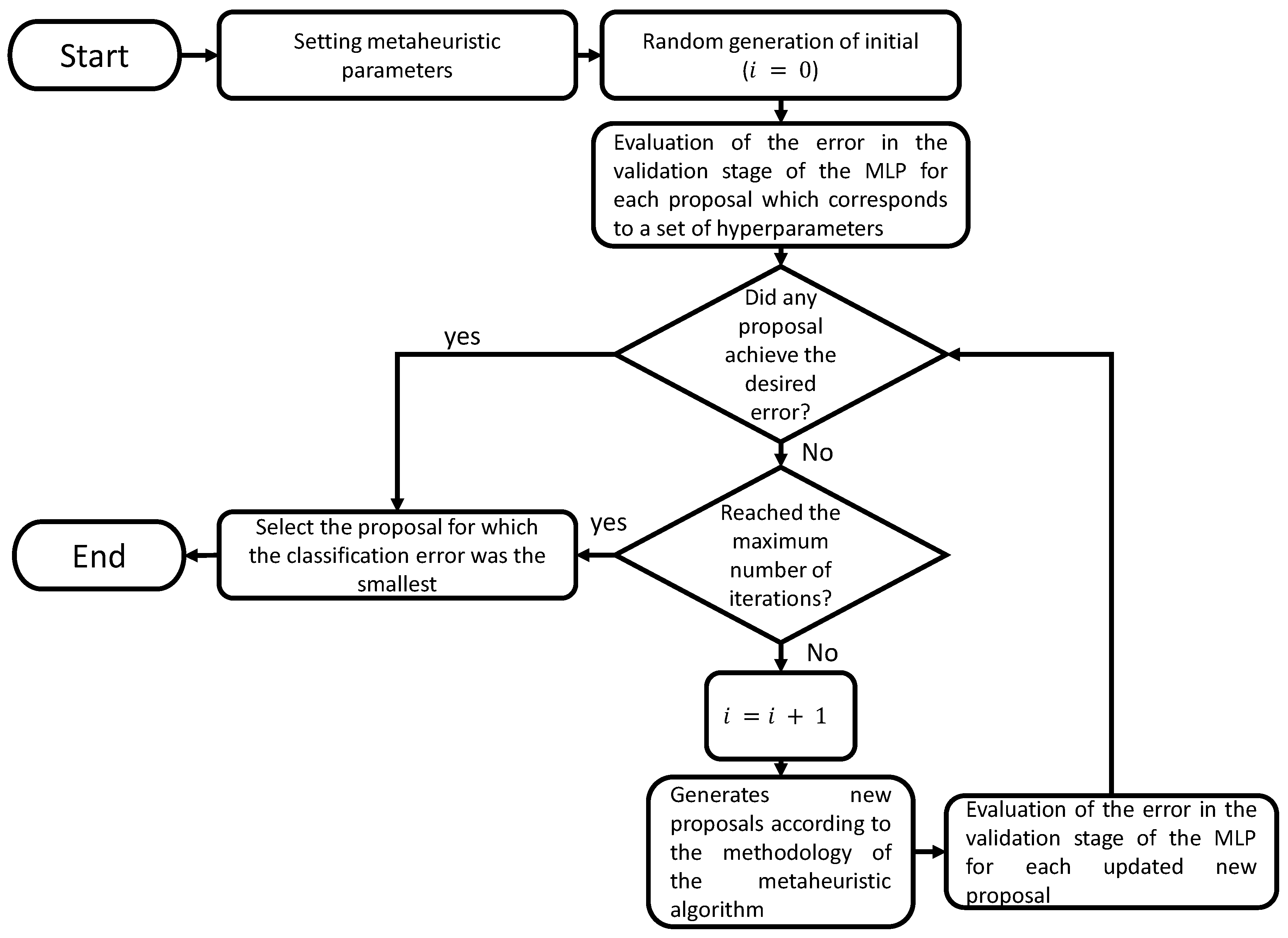
The different stages of the general methodology for integrating the PSO and GWO algorithm with an MLP neural network for hyperparameter selection are shown in Figure 2.

Figure 2. Proposal methodology for the selection of hyperparameters of MLP.

Figure 2. Proposal methodology for the selection of hyperparameters of MLP.

5. Results

This section presents and analyzes the results obtained from the multiple stages of the methodology.

5.1. Feature selection

Table 5 shows the characteristics the GA selected from 104 predictors. In total, 55 features were selected and used as inputs in an MLP to classify the data and select the hyperparameters, representing a 47% reduction in features. Achieving a final classification percentage of 93%.

Table 5. Features selected as the best subset of characteristics for classifying signals.

Acronym	Channel
AAC	1 and 2
IEMG	All
MAV	1, 2 and 4
MAVSLP	1 and 4
MMAV1	All
VAR	1, 2 and 4
FC	1, 2 and 4
K	1,2 and 4
Y3	1
MYOP	1, 3 and 4
AAV	2 and 4
DASDV	2 and 4
LOG	2 and 3
MMAV2	2 and 3
SSC	2
SSI	2, 3 and 4
STD	2, 3 and 4
WL	2, 4
ZC	2, 3 and 4
MAD	2, 3 and 4
WAMP	2, 3 and 4
SE	3
SK	3 and 4
RMS	4
Y4	4
Y5	4

Table 5. Features selected as the best subset of characteristics for classifying signals.

Acronym	Channel
AAC	1 and 2
IEMG	All
MAV	1, 2 and 4
MAVSLP	1 and 4
MMAV1	All
VAR	1, 2 and 4
FC	1, 2 and 4
K	1,2 and 4
Y3	1
MYOP	1, 3 and 4
AAV	2 and 4
DASDV	2 and 4
LOG	2 and 3
MMAV2	2 and 3
SSC	2
SSI	2, 3 and 4
STD	2, 3 and 4
WL	2, 4
ZC	2, 3 and 4
MAD	2, 3 and 4
WAMP	2, 3 and 4
SE	3
SK	3 and 4
RMS	4
Y4	4
Y5	4

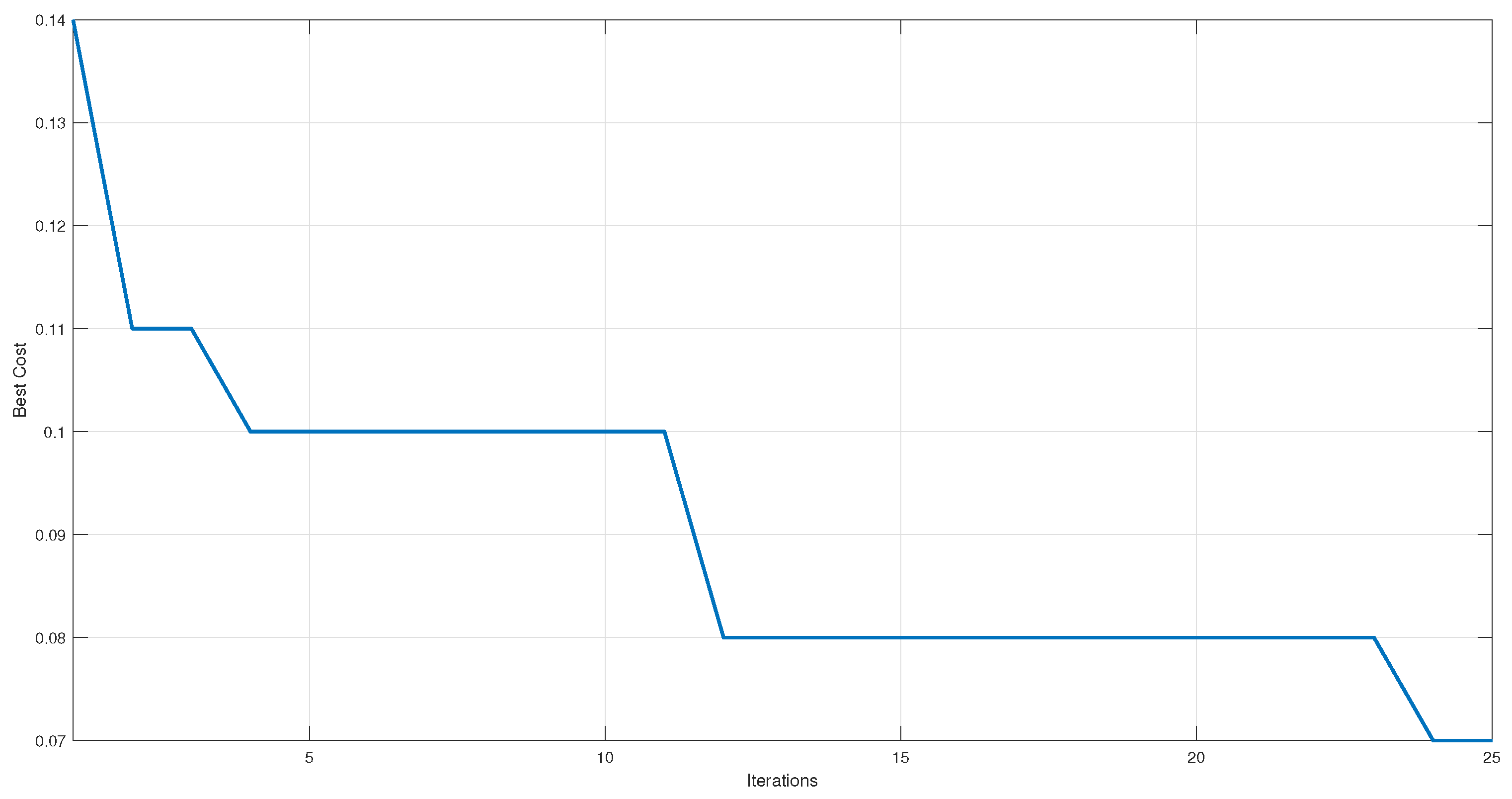
As shown in Figure 3 initially, the feature selection process had an error rate of 14%. The genetic algorithm improves performance during the first iterations and reduces errors to 11%. However, it stalls at a 10% error for 8 iterations and an 8% error for 12 iterations. This deadlock occurs when existing candidate solutions have already explored most of the search space and new feature combinations that significantly improve performance are not found. At this point, the genetic algorithm get stuck in a local minimum. This deadlock is overcome by implementing the mutate operation. In this case, it is possible that during the 10% error plateau period, some mutation introduced in a later iteration led to exploring a new combination of features that improved performance. This new solution could have been selected and propagated in the following generations, finally allowing it to reach a classification value of 93%.

Figure 3. Reduction of the classification error due to the selection of features through GA.

Figure 3. Reduction of the classification error due to the selection of features through GA.

In order to ensure that the feature selection process is carried out correctly and that only predictors that allow a high classification were selected, a sensitivity analysis was carried out. In Figure 4, the bar graph is shown where the percentages of decrease or increase in precision are observed concerning the classification obtained at the end of the character selection stage, which was 93%.

Figure 4. Sensitivity analysis of classification reduction percentages by predictor.

Figure 4. Sensitivity analysis of classification reduction percentages by predictor.

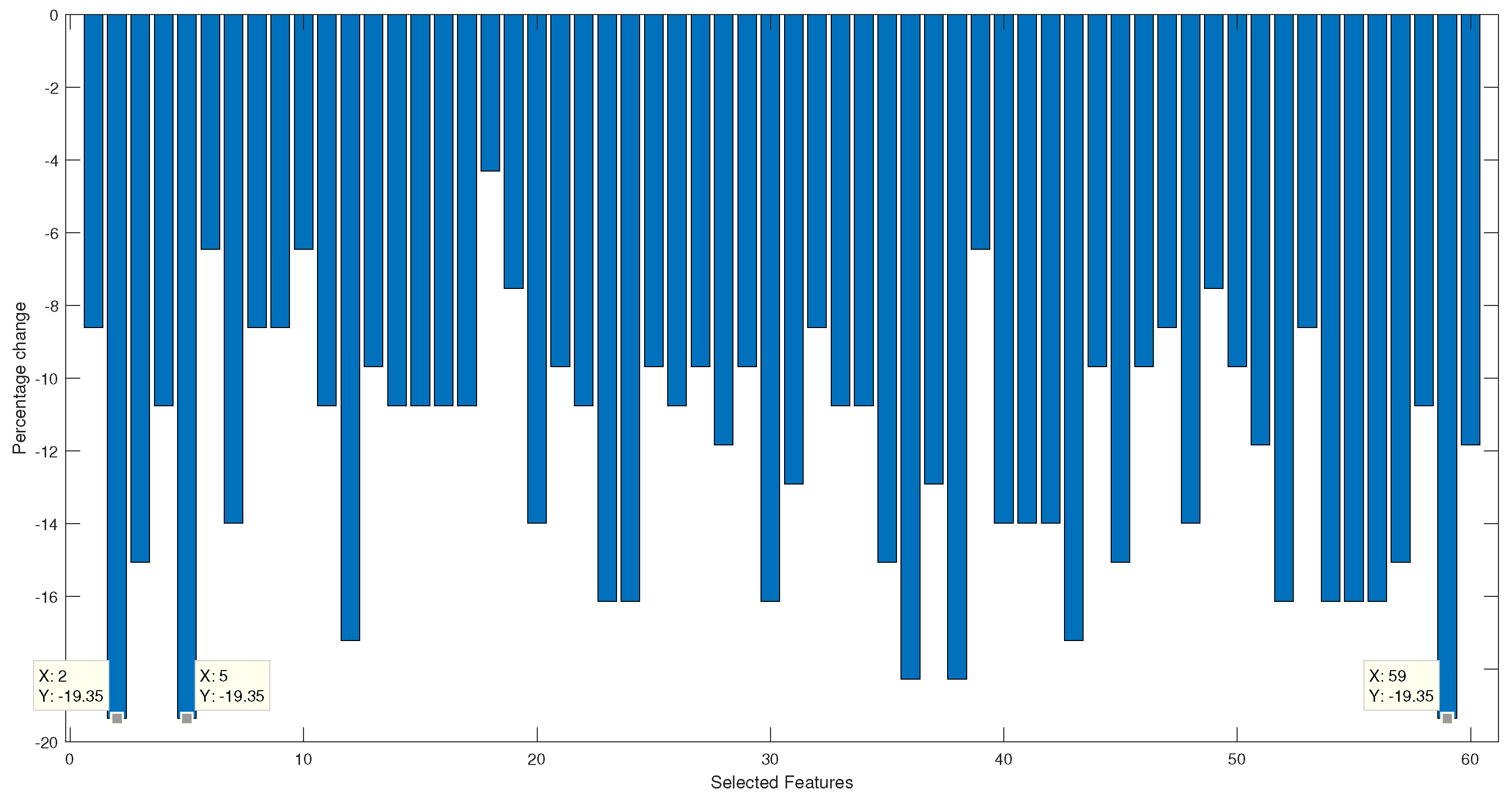
It is observed that feature number 18, which corresponds to the mean absolute value type 1 of channel 2, has the lowest percentage decrease in classification when eliminated. On the other hand, the characteristics with the most significant contribution are the absolute value of the fifth moment channel 4, integrated EMG channel 1, and modified mean value type 1 channel 1. When comparing the characteristics that present a more significant contribution against those of lesser contribution, it is seen that type 1 modified mean value appears in both limits. The difference occurs in the channel from which the characteristic is extracted. Therefore, the exact predictor can have more or less importance in the classification depending on the muscle from which it is extracted.

5.2. Hyperparameter selection

As shown in Figure 5 in the GWO implementation process, there is an error rate of 14% with the initial values proposed for the hyperparameters. This indicates that the initial solutions have yet to find the best set for the problem since, prior to the selection of hyperparameters, there is a classification percentage of 93%, and it is sought that the efficiency after the hyperparameter adjustment process is more significant or equal to the previous phase.

In iteration 4, a reduction in error to 7% is observed. The proposed solutions have found a hyperparameter configuration that improves model performance and reduces error. During subsequent iterations, they continue to adjust their positions and explore the search space for better solutions. As observed during iterations 5 to 20, a deadlock is generated. However, later it is observed that the error drops to 3%, which indicates that the GWO has managed to overcome this impasse and find a solution that considerably improves the classification.

A possible reason why the GWO managed to get out of the deadlock and reduce the error may be related to the intensification and diversification of the search. During the first few iterations, the GWO may have been in an intensification phase, focusing on exploiting promising regions of the search space based on the positions of the pack leaders. However, after a while, the GWO may have moved into a diversification phase, where the gray wolves explored new regions of the search space, allowing them to find a better solution and reduce the error to 3%.

Figure 5. Reduction of the error due to the selection of hyperparameters by GWO.

Figure 5. Reduction of the error due to the selection of hyperparameters by GWO.

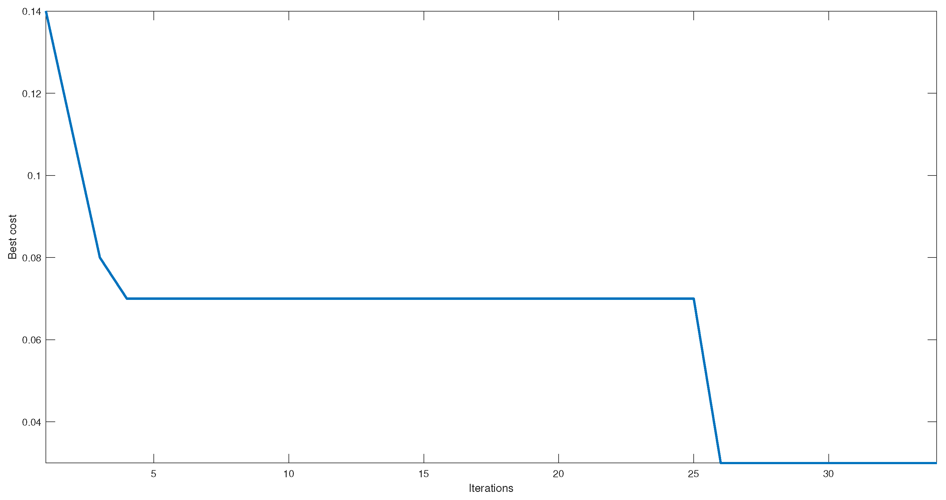
Table 6 shows the values obtained for the MLP hyperparameters using GWO, achieving a classification in the validation stage of 97%. When comparing the values implemented in the feature layer, it stands out that the number of hidden layers was reduced from 4 to 2. On the other hand, the total number of neurons was reduced from 600 to 409. However, epochs increased from 10 to 33 after hyperparameter selection. This indicates that the model required more opportunities to adjust the weights and improve its performance on the training data set. Similarly, the mini-batch size has been increased from 20 to 58, indicating that it needs more information during each training stage to adjust the weights.

Finally, the learning rate increased from 0.0001 to 0.002237, which showed that the neural network learned faster during training. The results indicate that the selection of hyperparameters improved the efficiency of the model by reducing its complexity without compromising its classification ability.

Table 6. Hyperparameters selected as the best subset for classifying signals given by GWO.

Name	value
Hidden neurons layer 1	204
Hidden neurons layer 2	205
Epochs	33
Mini-batch size	58
Learning rate	0.00223750

Table 6. Hyperparameters selected as the best subset for classifying signals given by GWO.

Name	value
Hidden neurons layer 1	204
Hidden neurons layer 2	205
Epochs	33
Mini-batch size	58
Learning rate	0.00223750

Figure 6 shows the error reduction in selecting hyperparameters by PSO. The best initial proposal achieves a 13% error. After this, there is a stage where the error percentage is kept constant until iteration 6. From there, the error is reduced to 8%. Once this error is reached, it remains constant until iteration 27. Once iteration 28 enters, an error of 7% is achieved, representing only a 1% improvement. This 1% improvement is not a significant increase and could be attributed to slight variations in MLP training weights.

Figure 6. Reduction of the error due to the selection of hyperparameters by PSO.

Figure 6. Reduction of the error due to the selection of hyperparameters by PSO.

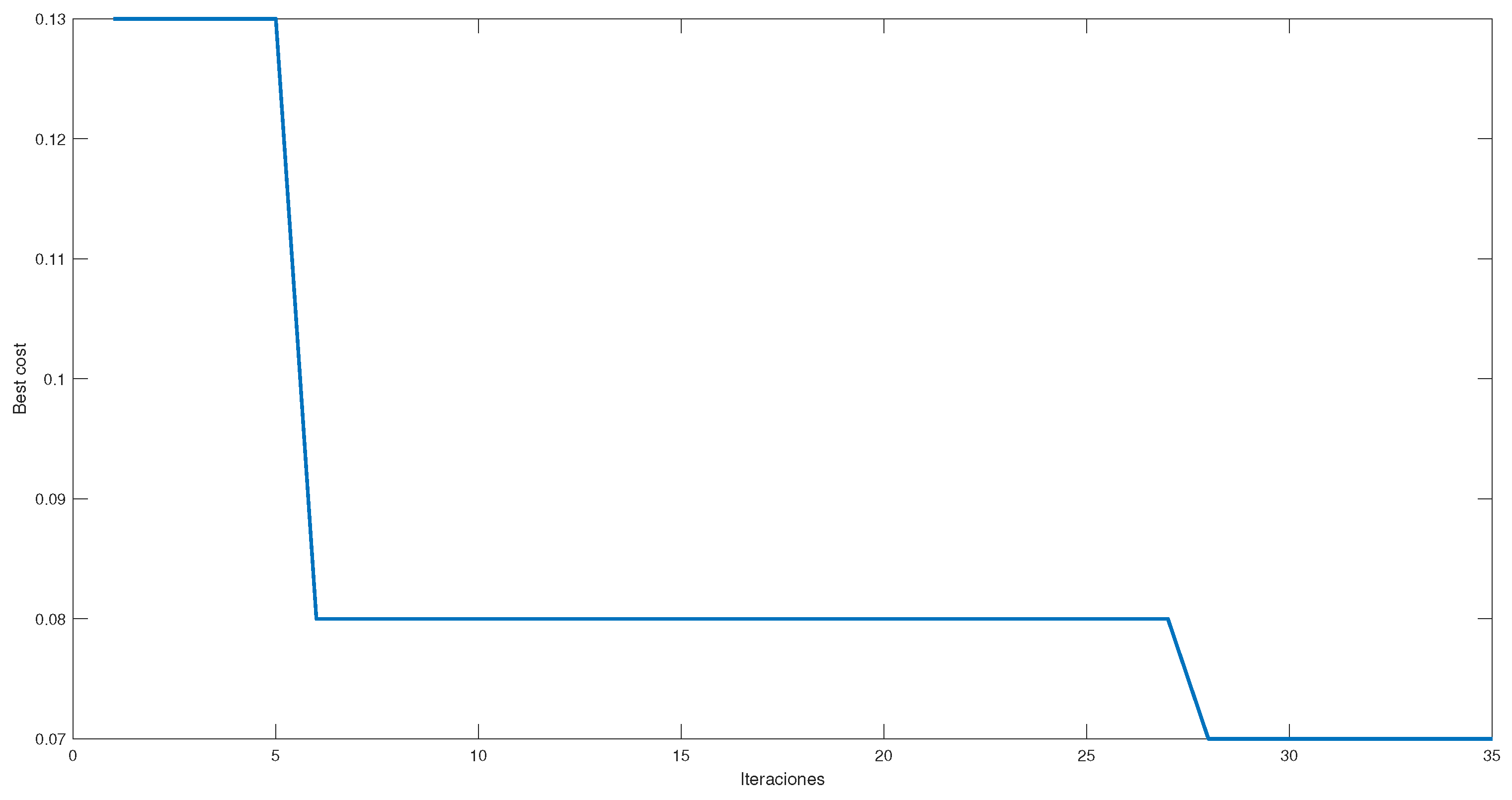
On the other hand, Table 7 shows the calculated values of the MLP hyperparameters through PSO; the precision achieved is less than that achieved by GWO, being 93%. Despite them, a 50% reduction in hidden layers is also achieved, and it manages to maintain the precision percentage obtained in the feature selection stage with fewer neurons than those achieved by GWO, being 359. However, similarly to the values obtained by GWO, epochs increased to 38. Similarly, the mini-batch size was increased from 50. Finally, the learning rate increased from 0.0001 to 0.0010184. This smaller amount of information used for training and the smaller learning steps, and the smaller number of neurons justifies the 4% decrease in the classification.

Table 7. Hyperparameters selected as the best subset for classifying signals given by PSO.

Name	value
Hidden neurons layer 1	155
Hidden neurons layer 2	204
Epochs	38
Mini-batch size	46
Learning rate	0.0010184

Table 7. Hyperparameters selected as the best subset for classifying signals given by PSO.

Name	value
Hidden neurons layer 1	155
Hidden neurons layer 2	204
Epochs	38
Mini-batch size	46
Learning rate	0.0010184

When comparing Figure 5 and Figure 6, it is observed that both start with error values close to 15%, and after the first iterations, it has an improvement close to 50%, achieving an error close to 8%. Hence both algorithms have a period of stagnation from which GWO get superior by getting a second improvement of 50% achieving errors of 3%. On the other hand, even though visually PSO managed to get out of stagnation, it only managed to reduce the error to 1%, which does not represent a significant improvement and can be attributed to variations within the MLP parameters such as weights and not to the selection of hyperparameters.

5.3. Validation

After selecting characteristics and hyperparameters, the rest of the ten that comprise the database were used to validate the results obtained since this information had never been used before. Figure 7 shows the graphs of the error in the training stage (60% of the data corresponding to 9 of 10 people, equivalent to 600 data to be classified), the test stage (40% of the data corresponding to 9 out of 10 people, equivalent to 200 data to classify) and validation stage that corresponds to data from the tenth person (equivalent to 100 data). It is noted that the data to be classified is formed from the number of people ×, the number of movements × the number of repetitions.

Figure 7. The error in training, testing, and validating a model using a) GWO hyperparameters and b) PSO hyperparameter.

Figure 7. The error in training, testing, and validating a model using a) GWO hyperparameters and b) PSO hyperparameter.

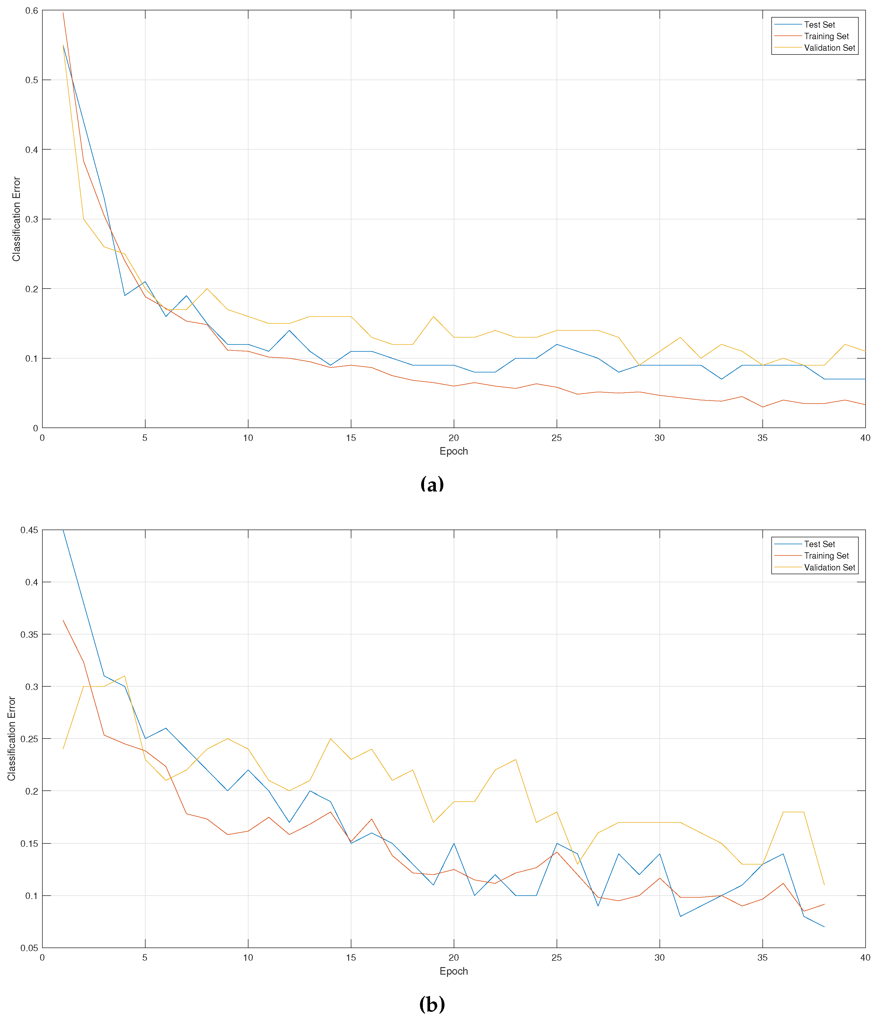
Additionally, these graphs allow us to verify the overfitting in the model. The training, test, and validation errors were plotted in each epoch. If the training error decreases while the test and validation errors increase, this suggests the presence of overfitting. However, the results indicated that the errors decreased evenly across the three stages, suggesting that the model generalize and classify accurately without overfitting. In addition, the percentage for the hyperparameter values given by GWO only decreased by approximately 4% for new input data, reaching 93% accuracy. While for PSO, 3% was lost in the classification, achieving a final average close to 90%.

6. Discussion

The following comparative Table 8 presents the classification results obtained in previews papers related to the subject of the study compared to the results obtained in this work.

Table 8. Comparative analysis of classification results.

Ref.	Classification model	Accuracy
[14]	SVM	91%
[15]	SVM	90.92%
[13]	SVM	97.5%
[10]	Recurrent neuronal network	95.7%
[8]	SVM	88%
This work	MLP	93%

Table 8. Comparative analysis of classification results.

Ref.	Classification model	Accuracy
[14]	SVM	91%
[15]	SVM	90.92%
[13]	SVM	97.5%
[10]	Recurrent neuronal network	95.7%
[8]	SVM	88%
This work	MLP	93%

In this work, an approach based on hyperparameter optimization using PSO and GWO was used to improve the performance of a multilayer perceptron in the classification of electromyographic signals. This approach perform comparably to other previously studied methods.

However, during the experimentation, there were stages of stagnation. Several reasons explain this lack of success. First, the intrinsic limitations of PSO and GWO, such as their susceptibility to stagnation at local optima and their difficulty in exploring complex search spaces, might have made it challenging to obtain the right combination of hyperparameters [29]. Other factors that might have played a role include the size and quality of the data set used since the multilayer perceptron requires a more considerable amount of data to generalize [30].

Despite these limitations, the proposed approach has several advantages. On the one hand, it allows to improve the performance of the multilayer perceptron by optimizing the key hyperparameters, which is crucial to obtain a more efficient model. Although the performance is comparable with other methods, the metaheuristics-based approach manages to reduce the complexity of the model, indicating its potential as an effective strategy for classifying electromyographic signals.

Furthermore, using PSO and GWO for hyperparameter optimization offers a systematic and automated methodology, making it easy to apply to different data sets and similar problems. It avoids manually tuning hyperparameters, which is messy and error-prone.

It is important to note that each method has its advantages and limitations, and the appropriate approach may depend on factors such as the size and quality of the data set, the complexity of the problem, and the available computational resources.

7. Conclusions

Properly selecting hyperparameters in MLP is crucial to correctly classifying EMG signals. Optimizing these hyperparameters is challenging due to the many possible combinations. This work uses the PSO and GWA algorithms to find the best combination of hyperparameters for the neural network.

Although 93% accuracy has been achieved in classifying EMG signals, there is still room for improvement. Some possible factors that have prevented higher accuracy may be the lack of training data and the variability of EMG signals. One way to overcome these problems, more training data might be retrieved and data augmentation techniques to be used to generate more variety in the signals.

Another possible solution might be using more advanced EMG signal preprocessing techniques to reduce noise and interference from unwanted signals. Different neural network architectures and optimization techniques might also be tested to improve the classification accuracy further.

In addition, it is essential to highlight that in this work, no normalization of the data was performed, which might have further improved the performance of the MLP model. Therefore, it is recommended to consider this step in future work to achieve better performance in classifying EMG signals.

It is essential to highlight that choosing the cost function used in metaheuristics algorithms is crucial for its success. In this work, the error in the validation stage of the neural network was used as the cost function to be minimized. However, alternatives include sensitivity, efficiency, specificity, ROC, and AUC.

Consequently, the choice of the cost function to be used in the metaheuristics algorithms must be carefully considered depending on the specific objectives of the problem being addressed. A cost function that works well in one issue may not work well in another. Therefore, exploring different cost functions and evaluating their performance is advisable before making a final decision.

Another factor that should be considered in this work is the initialization methodology of the network weights. Such considerations and initialization alternatives are within future work that must be analyzed.

In general, the selection of hyperparameters is a fundamental step in the construction and training of neural networks for the classification of EMG signals. With proper optimization of these hyperparameters and continuous exploration of new techniques and methods, significant advances are made in this area of research.

References

- Jia, G.; Lam, H.K.; Ma, S.; Yang, Z.; Xu, Y.; Xiao, B. Classification of electromyographic hand gesture signals using modified fuzzy C-means clustering and two-step machine learning approach. IEEE Trans. Neural Syst. Rehabil. Eng. 2020, 28, 1428–1435. [Google Scholar] [CrossRef] [PubMed]
- Albahli, S.; Alhassan, F.; Albattah, W.; Khan, R.U. Handwritten digit recognition: Hyperparameters-based analysis. Appl. Sci. (Basel) 2020, 10, 5988. [Google Scholar] [CrossRef]
- Yang, L.; Shami, A. On hyperparameter optimization of machine learning algorithms: Theory and practice. Neurocomputing 2020, 415, 295–316. [Google Scholar] [CrossRef]
- Du, K.L.; Leung, C.S.; Mow, W.H.; Swamy, M.N.S. Perceptron: Learning, generalization, model selection, fault tolerance, and role in the deep learning era. Mathematics 2022, 10, 4730. [Google Scholar] [CrossRef]
- Vincent, A.M.; Jidesh, P. An improved hyperparameter optimization framework for AutoML systems using evolutionary algorithms. Sci. Rep. 2023, 13, 4737. [Google Scholar] [CrossRef]
- Mirjalili, S.; Mirjalili, S.M.; Lewis, A. Grey wolf optimizer. Adv. Eng. Softw. 2014, 69, 46–61. [Google Scholar] [CrossRef]
- Purushothaman, G.; Vikas, R. Identification of a feature selection based pattern recognition scheme for finger movement recognition from multichannel EMG signals. Australas. Phys. Eng. Sci. Med. 2018, 41, 549–559. [Google Scholar] [CrossRef]
- Too, J.; Abdullah, A.; Mohd Saad, N.; Tee, W. EMG feature selection and classification using a pbest-guide binary particle swarm optimization. Computation (Basel) 2019, 7. [Google Scholar] [CrossRef]
- Sui, X.; Wan, K.; Zhang, Y. Pattern recognition of SEMG based on wavelet packet transform and improved SVM. Optik (Stuttg.) 2019, 176, 228–235. [Google Scholar] [CrossRef]
- Xiu, K.; Xiafeng, Z.; Le, C.; Dan, Y.; Yixuan, F. EMG pattern recognition based on particle swarm optimization and recurrent neural network. Int. J. Perform. Eng. 2020, 16, 1404. [Google Scholar] [CrossRef]
- Bittibssi, T.M.; Zekry, A.H.; Genedy, M.A.; Maged, S.A. sEMG pattern recognition based on recurrent neural network. Biomed. Signal Process. Control 2021, 70, 103048. [Google Scholar] [CrossRef]
- Li, Q.; Zhang, A.; Li, Z.; Wu, Y. Improvement of EMG pattern recognition model performance in repeated uses by combining feature selection and incremental transfer learning. Front. Neurorobot. 2021, 15, 699174. [Google Scholar] [CrossRef] [PubMed]
- Cao, L.; Zhang, W.; Kan, X.; Yao, W. A novel adaptive mutation PSO optimized SVM algorithm for sEMG-based gesture recognition. Sci. Program. 2021, 2021, 1–13. [Google Scholar] [CrossRef]
- Aviles, M.; Sánchez-Reyes, L.M.; Fuentes-Aguilar, R.Q.; Toledo-Pérez, D.C.; Rodríguez-Reséndiz, J. A novel methodology for classifying EMG movements based on SVM and genetic algorithms. Micromachines (Basel) 2022, 13, 2108. [Google Scholar] [CrossRef] [PubMed]
- Dhindsa, I.S.; Gupta, R.; Agarwal, R. Binary particle swarm optimization-based feature selection for predicting the class of the knee angle from EMG signals in lower limb movements. Neurophysiology 2022, 53, 109–119. [Google Scholar] [CrossRef]
- Li, X.; Yang, Y.; Chen, H.; Yao, Y. Lower limb motion pattern recognition based on IWOA-SVM. Third International Conference on Computer Science and Communication Technology (ICCSCT 2022); Lu, Y.; Cheng, C., Eds. SPIE, 2022.
- Toledo-Pérez, D.C.; Rodríguez-Reséndiz, J.; Gómez-Loenzo, R.A.; Jauregui-Correa, J.C. Support vector machine-based EMG signal classification techniques: A review. Appl. Sci. (Basel) 2019, 9, 4402. [Google Scholar] [CrossRef]
- Raez, M.B.I.; Hussain, M.S.; Mohd-Yasin, F. Techniques of EMG signal analysis: detection, processing, classification and applications. Biol. Proced. Online 2006, 8, 11–35. [Google Scholar] [CrossRef]
- Bi, L.; Feleke, A.g.; Guan, C. A review on EMG-based motor intention prediction of continuous human upper limb motion for human-robot collaboration. Biomed. Signal Process. Control 2019, 51, 113–127. [Google Scholar] [CrossRef]
- Argatov, I. Artificial neural networks (ANNs) as a novel modeling technique in tribology. Front. Mech. Eng. 2019, 5. [Google Scholar] [CrossRef]
- Zemzami, M.; El Hami, N.; Itmi, M.; Hmina, N. A comparative study of three new parallel models based on the PSO algorithm. Int. J. Simul. Multidiscip. Des. Optim. 2020, 11. [Google Scholar] [CrossRef]
- Jain, M.; Saihjpal, V.; Singh, N.; Singh, S.B. An overview of variants and advancements of PSO algorithm. Appl. Sci. (Basel) 2022, 12, 8392. [Google Scholar] [CrossRef]
- Nematzadeh, S.; Kiani, F.; Torkamanian-Afshar, M.; Aydin, N. Tuning hyperparameters of machine learning algorithms and deep neural networks using metaheuristics: A bioinformatics study on biomedical and biological cases. Comput. Biol. Chem. 2022, 97, 107619. [Google Scholar] [CrossRef] [PubMed]
- Nanda, S.J.; Panda, G. A survey on nature inspired metaheuristic algorithms for partitional clustering. Swarm Evol. Comput. 2014, 16, 1–18. [Google Scholar] [CrossRef]
- Andonie, R. Hyperparameter optimization in learning systems. J Membr Comput 2019, 1, 279–291. [Google Scholar] [CrossRef]
- Asghari Oskoei, M.; Hu, H. Myoelectric control systems—A survey. Biomedical Signal Processing and Control 2007, 2, 275–294. [Google Scholar] [CrossRef]
- Clerc, M.; Kennedy, J. The particle swarm - explosion, stability, and convergence in a multidimensional complex space. IEEE Trans. Evol. Comput. 2002, 6, 58–73. [Google Scholar] [CrossRef]
- Tran, B.; Xue, B.; Zhang, M. Overview of particle swarm optimisation for feature selection in classification. In Lecture Notes in Computer Science; Lecture notes in computer science, Springer International Publishing: Cham, 2014; pp. 605–617. [Google Scholar]
- Dargan, S.; Kumar, M.; Ayyagari, M.R.; Kumar, G. A survey of deep learning and its applications: A new paradigm to machine learning. Arch. Comput. Methods Eng. 2020, 27, 1071–1092. [Google Scholar] [CrossRef]
Disclaimer/Publisher’s Note: The statements, opinions and data contained in all publications are solely those of the individual author(s) and contributor(s) and not of MDPI and/or the editor(s). MDPI and/or the editor(s) disclaim responsibility for any injury to people or property resulting from any ideas, methods, instructions or products referred to in the content. |
© 2023 by the authors. Licensee MDPI, Basel, Switzerland. This article is an open access article distributed under the terms and conditions of the Creative Commons Attribution (CC BY) license (http://creativecommons.org/licenses/by/4.0/).
Copyright: This open access article is published under a Creative Commons CC BY 4.0 license, which permit the free download, distribution, and reuse, provided that the author and preprint are cited in any reuse.