
Submitted:
30 January 2024
Posted:
31 January 2024
You are already at the latest version
Abstract
The storm 'Daniel' has caused the most severe flood phenomenon that Greece has ever experienced, with thousands of hectares of farmland submerged for days. This led to sediment deposition in the inundated areas, which significantly altered the chemical properties of the soil, as revealed by extensive soil sampling and laboratory analysis. Causal relationships between soil chemical properties and sediment deposition were extracted using the DirectLiNGAM algorithm. Results of causality analysis showed that the sediment deposition affected the CaCO3 concentration in the soil. Also, causal relationships were identified between CaCO3 and available phosphorus (P-Olsen), as well as between sediment deposit depth and available manganese. The quantified relationships between the soil variables were then used to generate data using a Multiple Linear Perceptron (MLP) regressor for various levels of deposit depth (0, 5, 10, 15, 20, 25 and 30 cm). Then linear regression equations were fitted across the different levels of deposit depth to determine the effect of deposit depth on CaCO3, P, and Mn. The results show that there is a linear slope of 0.12, -0.16, and 0.13, for CaCO3, P, and Mn with deposit depth, respectively. Statistical analysis indicates that corn growing in soils with sediment over 10 cm requires a 31.8% increase in P rate to prevent yield decline. Additional notifications regarding cropping strategies in the near future are also discussed.
Keywords:
causal machine learning
; soil analysis
; causal discovery
; crop fertilization
; flood
; agriculture
; deposition
; climate change
1. Introduction
According to recent reports, based on several years of observations by 27 national academies from the European Union (EU), Norway and Switzerland, the frequency of extreme weather events, including hydrological events, has increased by 60% in Europe over the past three decades. The largest increase has been observed in hydrological phenomena, such as floods, landslides, and avalanches [1,2]. Also, severe summer and late-spring floods occur more frequently the last years in Greece. Global warming might cause periods of heavy precipitation in Europe during the summer, which may lead to more frequent floods, even though summers may become drier on average [3,4].
On 5-7 September 2023, Thessaly was hit by a once in a 1000-year weather event where extreme rainfall (700 mm in 48 hours) caused extensive floods. By 7 September 2023 less than 60 hours after the rains started, 72,951 ha were inundated by flooding. The flood led to land loss due to erosion and resulted in the accumulation of sediment in various areas across the Thessaly plain. The storm 'Daniel' has caused an extended sediment deposition in the flooded areas, which in some cases reached 60 cm depth of deposit. Clearly, the 2023 crop season suffered significant impacts due to flooding. The floods destroyed annual crops just before the harvest period like cotton and corn, other vegetable crops, clover (mainly alfalfa), but also industrial tomato (medium-late varieties). Permanent vine plantations and tree crops such as olives, apples, pears, almonds, pistachios, walnuts, peaches, kiwis, etc. were also suffered by extensive damage. Moving forward, it is crucial to educate farmers about the flood's influence on soil chemistry. This is especially important because numerous fields experienced substantial soil deposition. Understanding these changes is key for effective management in the upcoming crop season.
Focusing exclusively on correlation analysis, in the context of complex and multidimensional dataset coming from soil analysis, introduces significant obstacles. It is imperative to unravel the causal links instead of depending on correlations, which might arise from superficial associations among variables[5]. In essence, approaches that concentrate mainly on learning correlations to assess the influence of an environmental factor on soil quality often fall short in accurately capturing the real underlying dynamics. Statistical based methods fail to reveal the direct and indirect causal connections in data. They also face challenges in identifying and adjusting for potential biases[6].
In recent years, machine learning (ML) is extensively used in processing complex data like environmental or soil data, aiding in decision-making and forecasts, as noted by [7,8]. However, the effectiveness of these prediction models in environmental contexts is dependent on the dataset size. If there is not enough data available, then the models do not generalize well in varied settings. A key issue is that ML models often capture non-causal links between inputs and outputs, leading to reduced effectiveness in different environments [9].
Conducting controlled experiments is an effective way to identify and understand causal mechanisms for various natural phenomena [10]. However, performing controlled experiments is often impossible and expensive. Causal inference in general has become increasingly important in medicine and social science, as in many cases it is ethically impossible to experiment to discover or understand the causal mechanisms of various factors affecting life[11]. Causal machine learning may likely play a significant role in the field of environmental sciences, particularly considering the complexity of variables affecting nutrient availability in soil, the high dimensionality of soil data and the extensive nature of agriculture. To estimate the causal effect of sediment deposit on the soil chemical properties, directed acyclic graphs (DAGs) were employed to delineate potential causal connections among variables, aiding in creating a more universally applicable prediction model for the effect of sediment deposit on the chemical properties of the soil. Fehr [9] suggests that prediction accuracy improves in diverse settings when the models are based on causal factors rather than resultant elements of the predicted variable. Causal Machine Learning (CML) introduces a deeper layer of comprehension to the system enhancing general applicability and explicability of existing ML frameworks [6].
While correlation analysis is the most popular statistical tool to understand the relations among soil variables, it is not appropriate in the context of this study because our objective extends beyond simply examining the relationships between the soil variables, but also to explore whether sediment deposit has caused change in the soil chemistry [12]. Thus, our objectives in the current work are to assess the impact of sediment deposition on the soil chemical properties and formulate management strategies to prevent yield loss in the upcoming crop season.
2. Materials and Methods
A combination of Copernicus Sentinel satellite images, i.e. Sentinel-1 and Sentinel-2, was utilized for monitoring the flood [13]. Sentinel-1 is a radar satellite mission designed to provide all-weather, day-and-night imaging capabilities. It is particularly useful for monitoring natural disasters like floods, as it can penetrate cloud cover and gather data on surface conditions. Sentinel-2 is a multispectral imaging satellite mission designed to provide high-resolution optical imagery. It can capture detailed visual information about the Earth's surface. The combination of radar data from Sentinel-1 and optical imagery from Sentinel-2 offers a comprehensive view of the flood-affected regions. These Copernicus Sentinel satellites are part of the European Union's Copernicus Earth Observation program, which aims to provide accurate and timely information for environmental monitoring, emergency response, and other Earth observation applications. The use of both radar and optical satellite data allows for a more thorough analysis of the flood event, encompassing both the physical presence of water and the visual changes in the landscape caused by the inundation. Monitoring via satellite imagery for identifying and delineating the affected areas, revealed that severe inundation occurred in Karditsa, Larissa and Lake Karla areas, as shown in Figure 1. The flood has caused an extended sediment deposition in the flooded areas, as shown in Figure 2.
2.1. Soil Sampling and Analysis
Composite soil samples (three subsamples from 1 × 1 m surface area were mixed to make a composite soil sample) were extracted to a depth of 30 cm from 321 locations in the area impacted by the flooding. Immediately after the floodwaters receded, the soil samples were collected from the surface at each site. Out of these, 217 samples originated from areas without any sediment coverage, while 104 were gathered from fields with sediment layers varying between 1 and 60 cm in depth. The soil samples were air-dried and sieved following standard procedures. The soil samples analyzed for soil fertility (macro and micro-elemental analysis) and other basic soil physicochemical parameters with standard internationally recognized methods at the accredited laboratory of Soil, Plant and Water analyses of the Institute of Industrial and Forage Crops of the Hellenic Agricultural Organization "DIMITRA". The analysis assessed 18 soil parameters, including the weight percentage of sand, clay, and silt, soil pH, electrical conductivity (EC), soil organic matter content (SOM), calcium carbonate content (CaCO3), organic carbon (C), total nitrogen (N), phosphorus (P), potassium (K), sodium (Na), magnesium (Mg), iron (Fe), zinc (Zn), manganese (Mn), copper (Cu), and calcium (Ca) levels. The pH and EC values were measured using a soil-to-water ratio of 1:1 with specific meters [14,15]. Total nitrogen was quantified via the Kjeldahl technique [16], while C and SOM were determined by the Walkley-Black method [17]. CaCO3 content was assessed by titration [18], and soil texture was evaluated using the Bouyoucos hydrometer approach [19]. The Olsen method was employed for P [20]. The ammonium acetate extraction method followed by an atomic absorption spectrophotometer reading was used for Na, K, Ca, and Mg [21] Additionally, Mn, Cu, Fe, and Zn were extracted using DTPA and quantified with an atomic absorption spectrophotometer [22]
2.2. Data Preprocessing
The dataset analyzed to assess the impact of sediment on soil chemistry, after excluding missing data, comprised 296 entries. The dataset was randomly divided into a training set (80%, or 237 entries) and a test set (20%, or 59 entries). To reduce dimensionality and filter out insignificant attributes, the random forest algorithm was employed [23]. This step led to the exclusion of variables deemed of low importance based on the feature importance scores derived from the random forest model [24]. The remaining variables from the initial set were then examined for collinearity using Spearman’s rank correlation. Features that were found less critical by the random forest model and did not significantly increase error rates were removed [25].
2.3. Machine Learning
A LightGBM regressor was utilized to establish a relationship between soil deposit depth and the soil variables [26]. The algorithm was used to identify the relative importance of each variable on deposit depth. The LightGBM regressor was selected as it is a dynamic ML technique delivering state-of-the-art results in the ML framework [27]. The advantage of this technique is that it provides a refined sample splitting approach that minimizes the risk of overfitting. Additionally, its gradient-based one-side sampling (GOSS) is an innovative feature. GOSS prioritizes samples with larger gradients while randomly selecting those with smaller gradients, enhancing the algorithm’s efficiency and accuracy [26] The efficiency of the LightGBM algorithm depends a lot on the optimal selection of the hyperparameters, because it uses the gradient boosting framework and is prone to overfitting. The Optuna library was used for hyperparameter tuning of the LightGBM algorithm [28]. 100 trials with different combinations of hyperparameters were tested and the combination of parameters that minimized the Mean Absolute Error (MAE) was selected. The optimum hyperparameter values for the LightGBM model were as follows:
- learning_rate=0.02, num_leaves=662, subsample=0.2, colsample_bytree=0.63, and min_data_in_leaf =15.
2.4. SHAP Analysis
To elucidate the factors related to deposit depth as determined by the LightGBM model, Shapley Additive Explanations (SHAP) analysis was implemented [29,30]. SHAP, an Explainable Artificial Intelligence (XAI) approach, draws from game theory and quantifies a feature's effect on a model's output [31,32]. It calculates a Shapley value for each prediction by altering the input data across all rows for one feature per test, while keeping the remaining data consistent with the original. Each SHAP value, thus computed individually for every prediction, elucidates that specific prediction. It does so by assessing the deviation from the model’s forecast to that obtained by altering a single feature. A significantly positive sum of these deviations suggests a strong positive influence of the feature on that prediction. Conversely, a highly negative sum indicates a negative influence, while a sum near zero implies the feature's minimal impact. Practically, SHAP constructs a small explainer model for each observation, explaining the rationale behind the model's prediction for that case [33]. This is especially useful for nonlinear methods like LightGBM. While this algorithm is effective in reducing prediction errors, discerning the logic behind their outputs is often challenging. For visualization purposes, the SHAP library was utilized to create graphical representations of feature importance and SHAP dependency plots.
2.5. Casual Representation, Discovery and Reasoning
Causal models offer insights into the generative processes involved in the creation of the data, going beyond mere correlations between the variables[34]. Causal representation involves the understanding of the causal relationship between the variables. Causal discovery is the process of discovering causal links between the variables, while causal reasoning focuses on estimating the impact of the interventions between the variables [6] In DAGs, each node symbolizes a variable, while the directed edges indicate direct causal influences, with the arrow pointing from the cause to its subsequent effect [9,35]. A (DAGs) was employed to map the causal connections among the variables. Initially, the Direct Linear non-Gaussian acyclic model (DirectLiNGAM) was employed to map the causal links between the variables. The DirectLiNGAM algorithm is an improvement of the LiNGAM algorithm, as it can estimate more robustly the causal structure in the data, if data does not strictly meet the non-Gaussianity assumption of the original LiNGAM algorithm. DirectLiNGAM assumes that the actual causal connection in the data is linear, acyclic, and without any hidden confounders. It also introduces an improved method for estimating the causal order in the variables, which is characterized by three key steps: pairwise causality tests, estimation of the causal ordering based on the pairwise tests, and estimation of the connection strengths. In general, the assumption of non-Gaussianity (data non-Gaussian distributed) enables the LiNGAM algorithm to extend beyond second-order statistical analysis, such as the covariance, to fully uncover the causal structure within the data [11,12,36].
Subsequently, the Regression with Subsequent Independence Test (RESIT) was employed to illustrate the impact of sediment deposition on soil chemistry. Proposed by Hoyer et al. [37] and Peters et al. [38] RESIT is recognized as a method for non-linear causal discovery, capable of discerning causal structures under the assumption of non-linearity. The RESIT method is based on the principle that if X causes Y, then after regressing Y on X, the residuals should be independent of X. There are three steps in this procedure: a regression is performed between Y and X to predict Y based on X, the residuals representing the part of Y not explained by X are computed and a kernel-based conditional independence test is performed between X and the residuals [39]. For this study, the RESIT algorithm incorporated a Multiple Linear Perceptron (MLP) regressor for its implementation instead of a simple linear regression, as MLP is a non-linear model and particularly useful for complex data coming from soil analysis. The confidence level for the different deposit depths was obtained by bootstrapping the dataset 10 times using the multiscale bootstrap method. The multiscale bootstrap method gives unbiased p-values with much higher statistical reliability [40]
Following this, data were generated based on the causal relationships of the soil data. A MLP regressor was used to fit the causal data generator producing datasets for varying sediment deposit depth (0, 5, 10, 15, 20, 25 and 30 cm). Then, linear regression equations were fitted to determine the trends of increase in CaCO3 and Mn increase and the decrease in P in relation to these deposit depth levels.
3. Results
3.1. Causal Inference
Soil analysis shows significant impact of sediment depth on the soil chemical properties. Thus, spearman test showed significant positive correlation between deposit depth and CaCO3 (p<0.001), Mn (p<0.001), Fe (p<0.001), Cu (p<0.007) and pH (p<0.009), and a negative correlation with K (p<0.004). Indeed, as demonstrated in the histograms of Figure 3, elevated levels of Cu, Fe, and Mn are predominantly found in soil deposits. Causal data analysis suggests that deposit depth affects CaCO3 content in soil chemistry and there is a causal link between Mn and deposit depth, and a causal link exists also between CaCO3 with P and Fe (Figure 4). DAG in Figure 4 also shows that the deposit depth affects the physical properties of the soil leading to an increase in sand content and in a reduction to the ratio of organic carbon to total nitrogen content. Some estimated relationships, however, were controversial to the domain knowledge, as, for example, the causal link between CaCO3 and P has obviously the opposite direction. This is clearly also true for the causal link between Mn and deposit depth, as the effect of deposit has caused Mn to increase and not the opposite.
The RESIT algorithm was used to obtain the confidence level for the various sediment depths. Figure 5 (a) shows that for deposit depth higher than 10 cm CaCO3 increased significantly compared to soils with no sediment deposit. Figure 5 (b) additionally indicates that for a deposit depth exceeding 20 cm, P concentrations are significantly lower compared to soils without sediment. Figure 5 (c) demonstrates deposit depth resulted in significantly higher Mn concentration, while Figure 5 (d) shows that Fe levels were not affected by soil deposit.
Generated data based on the causal relationships using an MLP regressor provided datasets for various levels of deposit depths (0, 5, 10, 15, 20, 25 and 30 cm). Regression equations showed that CaCO3 and Mn increase in relation to the sediment depths according to the following equations (Figure 6):
while P decreases in relation to sediment depth according to the following equation:
CaCO3: y=0.12x+6.19, (R2=0.99)
Mn: y=0.13x+22.21, (R2=0.95)
P: y=-0.16x+11.78, (R2=0.94)
However, the confidence intervals were only obtained by bootstrapping and shown in Figure 5.
3.2. Machine Learning and SHAP Analysis
A prediction model was developed using a LightGBM regressor, where the target variable was the deposit depth, and the input variables were the soil analysis data. The prediction model was trained to identify the relative importance of each variable on deposit depth. The MAE of the model is equal to 5.37 cm of deposit depth. The feature importance plot for the LightGBM model is presented in Figure 7. CaCO3, P, Mn are the most important features for the LightGBM model.
The SHAP dependence plots reveal that variables exhibiting highly significant correlations based on the Spearman test (p<0.001), namely CaCO3, Fe, and Mn, demonstrate an upward trend as deposit depth increases, as depicted in Figure 8 (a), (c), and (d). However, it is noteworthy that the normalized SHAP values indicate a narrower range of increase for Fe (-0.2 to 0.8) in comparison to the other variables. Consequently, CaCO3 and Mn hold higher positions in the feature importance plot (Figure 7), while Fe ranks low in the importance score. P, which has a connection with CaCO3, as demonstrated by the DirectLiNGAM algorithm (Figure 4), ranks second in the feature importance score (Figure 7) and decreases with increasing deposit depth. The primary interactions related to CaCO3, P, Mn, and Fe are C to N ratio with CaCO3, pH with P, N with Mn, and N with Fe. (Figure 8). It is worth noting that the C to N ratio exhibits a negative correlation with soil deposit due to a significant increase in N within the soil deposit, as illustrated in Figure 7.
3.3. Crop phosphorus Fertilizer Rate for Soils with Sediments
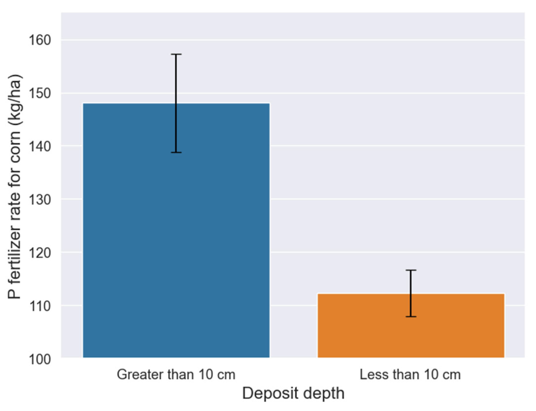
The Soil and Water Resources Institute's Fertilization Advisory Software (FAS) was utilized to assess the P needs for corn in Thessaly, a crop commonly cultivated in the region. FAS integrates an equation for calculating the P fertilizer rate, which includes factors like soil texture, CaCO3 content, Soil Organic Matter (SOM), available P, pH, and the specific P requirements of crops to achieve maximum yield[44]. As statistical differences of CaCO3 levels were observed for soil deposits above 10 cm (Figure 5 (a)), data were binned in two groups: soil deposits with less or more than 10 cm. This categorization was also driven by the observed variance in P needs for soils without deposits, ranging from completely depleted to highly available P, which is a normal finding in agricultural soils. The Shapiro test indicated non-normal variance in these groups. Thus, Kruskal-Wallis test was carried out to test the difference between the two groups [45]. The analysis showed that 31.8% higher P fertilizer rates are needed for soils with greater than 10 cm sediments for avoiding yield reduction of corn (p=0.001).
4. Discussion
This study conducts a causal discovery between soil variables to trace the effect of sediment deposition on soil chemistry. The causal discovery algorithms presented in this study (DirectLiNGAM and RESIT) were capable to capture the effect of soil deposit on the soil chemistry, as they are an evolution of the traditional causal algorithms employing the assumption on non-Gaussianity and non-linear causal discovery for DirectLiNGAM and RESIT, respectively. The results revealed a noteworthy effect of soil deposit on CaCO3 content, which indirectly affected the P levels. Causal analysis in Figure 5 shows that there is a downward trend of P concentration in relation to deposit depth and the difference is significant for soil having deposits greater than 20 cm compared to soils without deposits. The LightGBM algorithm confirms also that there is a downward trend, but it is less conservative compared to the RESIT algorithm, as it finds that for soils with sediments it is unlikely to have higher than 10 mg/kg P concentration (Figure 8). Interestingly, although P was identified as the second most influential factor by the LightGBM algorithm, the Spearman correlation analysis did not mark it as significant in relation to the deposit depth variable. This highlights the non-linear association between P levels and sediment presence.
Following nitrogen (N), P stands as a crucial nutrient essential for plant growth and overall productivity. Even though normally the soil contains P at levels around 2000 times higher than what's found in plants, its fixation in the form of aluminum/iron or calcium/magnesium phosphates renders it inaccessible for uptake by plants [20]. Consequently, plants frequently encounter the challenge of P deficiency in agricultural fields. Detecting this deficiency proves to be not an easy task, as crops typically do not exhibit visual symptoms during the early stages [46]. Thus, there is no consistent chlorosis observed in plants suffering from P deficiency. The shortage of P adversely affects plant growth, a consequence attributed to either a decrease in photosynthesis or an increase in energy investment. This limitation has a detrimental impact on both crop yield and quality. It is estimated that P deficiency leads to reduced crop yields on approximately 30-40% of the world's arable land. In agricultural fields, Phosphorus Use Efficiency (PUE) ranges around 15-20%, indicating that a significant portion of the P applied to the soil remains inaccessible for plant uptake [47]. The reduced P availability due to sediment deposition in the flooded areas necessitates the use of increased P rates for the next growing season in Thessaly.
Corn was used as a model crop for running FAS for all the soil samples taken by the study region. The analysis revealed that 31.8% higher P fertilizer rate is necessary to avoid yield reduction for corn in Thessaly for the next growing season (Figure 9). Fertilizer types that normally used in Thessaly for corn are the following: (N-P-K) 21-7-10, 18-10-22, and 33-10-7, according to the potassium levels at the various fields. The rate at broadcasting for these fertilizers is about 600 kg/ha. Thus, the P rate is 42 or 60 kg/ha according to the fertilizer type used, which is quite lower compared to the average 112 kg of P per ha suggested by FAS for soils without sediments. This necessitates extra care for applying higher rates for soils with sediments compared to the normally used in the Thessaly area.
Correlation analysis was not sufficient to explain the causality between soil deposit and changes in nutrient availability in the soil. Despite that a high spearman correlation was observed between soil deposit and Fe, which can also be confirmed by some high Fe values in soils having deposit (shown in the Fe histogram of Figure 3), causal analysis elucidated that Fe concentration in soil was not affected by the soil deposit. This result is also confirmed by the LightGBM algorithm, which classified Fe low in the feature importance score (Figure 7) for explaining soil deposit variability. The directed acyclic graph (DAG) in Figure 4, shows that the effect of CaCO3 is negative on Fe concentration in soil, which is known by the domain knowledge, as the formation of calcium-iron phosphate compounds in the presence of CaCO3 can reduce the availability of iron in the soil [48]. Thus, although there were some extreme Fe concentrations in the soil deposits, the presence of increased CaCO3 in the sediments resulted in the mitigation of iron in the soil, a trend which is also shown in Figure 5, as non-statistical differences were observed across the various deposit depths. This confirms that the existence of correlation between variables is necessary, but not sufficient condition for causality [12]
The Mn concentration though presents an upward trend with the increase of deposit depth, which was confirmed by both causal analysis and the LightGBM algorithm. However, even these increased levels of Mn, i.e. 45 mg/kg of soil (for the upward limit of the confidence interval at 30 cm deposit depth as shown in Figure 5) are not limiting plant growth. This highlights the effectiveness of bootstrapping with the RESIT algorithm, which enables the construction of confidence intervals at the various levels of deposit depth.
We found that some causal links between variables were controversial to domain knowledge. For example, CaCO3 affects P availability and not the opposite. This observation might likely stem from the limited size of the dataset. Nonetheless, the dataset size is inevitably small, considering the extensive effort required to collect these samples from the flooded region and to identify areas with sediments, especially given the narrow timeframe available for collecting samples before the growers incorporate the sediments in the soil.
Other causal links identified by the DirectLiNGAM algorithm included the effect of deposit depth on sand and the ratio of organic carbon to total nitrogen (C/N). As the feature importance plot shows, the negative effect of deposit depth on carbon to total N ratio is mostly because of the increase of total N content in the sediments (probably due to the transfer of floating organic matter together with the sediment). In addition to soil chemistry, it's crucial for farmers to manage the physical properties of soils affected by sediment deposition. The presence of fine, silty particles with small pores can lead to waterlogging, as these particles absorb water without allowing it to drain efficiently. This could result in difficulty in root function and restrict the aeration of the soil beneath. To mitigate these issues and ensure optimal crop production, it is essential to incorporate these sediments thoroughly with the existing soil, ensuring a homogeneous mixture that maintains the soil's physical properties.
5. Conclusions
Data presented here show that sediments caused a CaCO3 increase which indirectly caused a reduction in P availability. As a result, an increased P fertilizer rate recommendation is advisable for the next season’s crops grown in soils with sediments to avoid yield reductions. Considering that corn growers currently apply less P than what is optimal for maximum growth and yield, special attention is required for the next season's cultivation. CML has proven to be a valuable tool for determining the effect of sediments on soil chemistry, but most importantly the CML quantified the relationship between soil deposit, CaCO3, P, and Mn, by providing confidence intervals at various deposit depths, utilizing the established causal links within the data. The LightGBM algorithm confirmed the results of causal analysis, by identifying CaCO3 and P as the most influencing features for the deposit depth variable. Mn levels were found to increase significantly with increasing deposit depth, as indicated by the causal analysis. However, this increase remained within limits that are unlikely to restrict crop growth. The deposit led to a reduction in the C/N ratio, probably due to an elevation in N levels by the transfer of floating organic matter.
Author Contributions
Conceptualization, M.I., A.T., E.E., C.N., D.V. and P.T.; methodology, M.I.; software, M.I.; validation, M.I..; formal analysis, M.I.; investigation, M.I., A.T., E.E., C.N., D.V. and P.T.; resources, M.T, A.T., E.E., C.N., D.V.; data curation, M.I., V.A., and A.T.; writing—original draft preparation, M.I.; writing—review and editing, M.I., V.A., G.A., I.M. and C.K.; visualization, M.I., A.T. and P.T.; supervision, M.I.; project administration, D.V. and G.A.; funding acquisition, D.V. All authors have read and agreed to the published version of the manuscript.
Institutional Review Board Statement
Not applicable.
Data Availability Statement
The data can be made available by contacting the corresponding author.
Conflicts of Interest
The authors declare no conflict of interest.
References
- European Academies Science Advisory Council Extreme Weather Events in Europe Preparing for Climate Change Adaptation: An Update on EASAC’s 2013 Study;
- Furtak, K.; Wolińska, A. The Impact of Extreme Weather Events as a Consequence of Climate Change on the Soil Moisture and on the Quality of the Soil Environment and Agriculture – A Review. Catena (Amst) 2023, 231, 107378. [Google Scholar] [CrossRef]
- Loeb, R.; Lamers, L.P.M.; Roelofs, J.G.M. Effects of Winter versus Summer Flooding and Subsequent Desiccation on Soil Chemistry in a Riverine Hay Meadow. Geoderma 2008, 145, 84–90. [Google Scholar] [CrossRef]
- Christensen, J.H.; Christensen, O.B. Severe Summertime Flooding in Europe. Nature 2003, 421, 805–806. [Google Scholar] [CrossRef] [PubMed]
- Khatibi, E.; Abbasian, M.; Azimi, I.; Labbaf, S.; Feli, M.; Borelli, J.; Dutt, N.; Rahmani, A.M. Impact of COVID-19 Pandemic on Sleep Including HRV and Physical Activity as Mediators: A Causal ML Approach. In Proceedings of the 2023 IEEE 19th International Conference on Body Sensor Networks (BSN); 2023; pp. 1–4.
- Sanchez, P.; Voisey, J.P.; Xia, T.; Watson, H.I.; O’Neil, A.Q.; Tsaftaris, S.A. Causal Machine Learning for Healthcare and Precision Medicine. R Soc Open Sci 2022, 9. [Google Scholar] [CrossRef] [PubMed]
- Karydas, C.; Iatrou, M.; Kouretas, D.; Patouna, A.; Iatrou, G.; Lazos, N.; Gewehr, S.; Tseni, X.; Tekos, F.; Zartaloudis, Z.; et al. Prediction of Antioxidant Activity of Cherry Fruits from UAS Multispectral Imagery Using Machine Learning. Antioxidants (Basel) 2020, 9, 156. [Google Scholar] [CrossRef] [PubMed]
- Iatrou, M.; Karydas, C.; Iatrou, G.; Pitsiorlas, I.; Aschonitis, V.; Raptis, I.; Mpetas, S.; Kravvas, K.; Mourelatos, S. Topdressing Nitrogen Demand Prediction in Rice Crop Using Machine Learning Systems. Agriculture 2021, 11. [Google Scholar] [CrossRef]
- Fehr, J.; Piccininni, M.; Kurth, T.; Konigorski, S. Assessing the Transportability of Clinical Prediction Models for Cognitive Impairment Using Causal Models. BMC Med Res Methodol 2023, 23, 187. [Google Scholar] [CrossRef]
- Shimizu, S.; Inazumi, T.; Kawahara, Y.; Washio, T.; Hoyer PATRIKHOYER, P.O.; Bollen, K.; Sogawa, Y.; Hyvärinen, A.; Hoyer, P.O.; Bollen SHIMIZU, K. DirectLiNGAM: A Direct Method for Learning a Linear Non-Gaussian Structural Equation Model Yasuhiro Sogawa Aapo Hyvärinen; 2011; Vol. 12;
- Shimizu, S.; Inazumi, T.; Sogawa, Y.; Hyvärinen, A.; Kawahara, Y.; Washio, T.; Hoyer, P.O.; Bollen, K. DirectLiNGAM: A Direct Method for Learning a Linear Non-Gaussian Structural Equation Model. J. Mach. Learn. Res. 2011, 12, 1225–1248. [Google Scholar]
- Niyogi, D.; Kishtawal, C.; Tripathi, S.; Govindaraju, R.S. Observational Evidence That Agricultural Intensification and Land Use Change May Be Reducing the Indian Summer Monsoon Rainfall. Water Resour Res 2010, 46. [Google Scholar] [CrossRef]
- Copernicus Emergency Management Service Directorate Space, Security and Migration, European Commission Joint Research Centre (EC JRC).
- Miller, J.; Curtin, D. Electrical Conductivity and Soluble Ions.; 2007.
- Gavlak, R.G.; Horneck, D.A.; Miller, R.O. Plant, Soil, and Water Reference Methods for the Western Region; Western Rural Development Center, 1994;
- Pearson, D. The Chemical Analysis of Foods; 7th ed.; Churchill Livingstone, Edinburgh: London, UK, 1976.
- Walkley, A.; Black, I.A. AN EXAMINATION OF THE DEGTJAREFF METHOD FOR DETERMINING SOIL ORGANIC MATTER, AND A PROPOSED MODIFICATION OF THE CHROMIC ACID TITRATION METHOD. Soil Sci 1934, 37, 29–38. [Google Scholar] [CrossRef]
- van Reeuwijk, L.P. Procedures for Soil Analysis. 2002.
- Bouyoucos, G.J. Hydrometer Method Improved for Making Particle Size Analyses of Soils1. Agron J 1962, 54, 464–465. [Google Scholar] [CrossRef]
- Iatrou, M.; Papadopoulos, a.; Papadopoulos, F.; Dichala, O.; Psoma, P.; Bountla, a. Determination of Soil Available Phosphorus Using the Olsen and Mehlich 3 Methods for Greek Soils Having Variable Amounts of Calcium Carbonate. Commun Soil Sci Plant Anal 2014, 45, 2207–2214. [Google Scholar] [CrossRef]
- Knudsen, D.; Peterson, G.A.; Pratt, P.F. Lithium, Sodium, and Potassium. In Methods of Soil Analysis; Agronomy Monographs; 1983; pp. 225–246 ISBN 9780891189770.
- Iatrou, M.; Papadopoulos, A.; Papadopoulos, F.; Dichala, O.; Psoma, P.; Bountla, A. Determination of Soil-Available Micronutrients Using the DTPA and Mehlich 3 Methods for Greek Soils Having Variable Amounts of Calcium Carbonate. Commun Soil Sci Plant Anal 2015, 46, 1905–1912. [Google Scholar] [CrossRef]
- Breiman, L. Random Forests. Mach Learn 2001, 45, 5–32. [Google Scholar] [CrossRef]
- Howard, J.; Gugger, S. Deep Learning for Coders with Fastai and PyTorch; O’Reilly Media: Sebastopol, Canada, 2020. [Google Scholar]
- Howard, J.; Gugger, S. Fastai: A Layered API for Deep Learning. ArXiv 2020, abs/2002.0.
- Ke, G.; Meng, Q.; Finley, T.; Wang, T.; Chen, W.; Ma, W.; Ye, Q.; Liu, T.-Y. LightGBM: A Highly Efficient Gradient Boosting Decision Tree. In Proceedings of the Advances in Neural Information Processing Systems; Guyon, I., Luxburg, U. Von, Bengio, S., Wallach, H., Fergus, R., Vishwanathan, S., Garnett, R., Eds.; Curran Associates, Inc., 2017; Vol. 30.
- Iatrou, M.; Karydas, C.; Tseni, X.; Mourelatos, S. Representation Learning with a Variational Autoencoder for Predicting Nitrogen Requirement in Rice. Remote Sens (Basel) 2022, 14. [Google Scholar] [CrossRef]
- Akiba, T.; Sano, S.; Yanase, T.; Ohta, T.; Koyama, M. Optuna: {A} Next-Generation Hyperparameter Optimization Framework. CoRR 2019, abs/1907.1. [Google Scholar]
- Lundberg, S.M.; Lee, S.-I. A Unified Approach to Interpreting Model Predictions. CoRR 2017, abs/1705.0. [Google Scholar]
- Wojtuch, A.; Jankowski, R.; Podlewska, S. How Can SHAP Values Help to Shape Metabolic Stability of Chemical Compounds? J Cheminform 2021, 13, 74. [Google Scholar] [CrossRef] [PubMed]
- Lloyd, S. N-Person Games. Defense Tech. Inf. Cent. 1952, 295–314. [Google Scholar]
- Gramegna, A.; Giudici, P. SHAP and LIME: An Evaluation of Discriminative Power in Credit Risk. Frontiers in Artificial Intelligence 2021, 4. [Google Scholar] [CrossRef] [PubMed]
- Joseph, A. Shapley Regressions: A Framework for Statistical Inference on Machine Learning Models. ; 4th ed.; arxiv, 2019.
- Howard, R.; Kunze, L. Evaluating Temporal Observation-Based Causal Discovery Techniques Applied to Road Driver Behaviour. 2023.
- Pearl, J. Causal Diagrams for Empirical Research. Biometrika 1995, 82, 669–688. [Google Scholar] [CrossRef]
- Hyvärinen, A.; Smith, S.M.; Spirtes, P. Pairwise Likelihood Ratios for Estimation of Non-Gaussian Structural Equation Models;
- Hoyer, P.O.; Janzing, D.; Mooij, J.; Peters, J.; Schölkopf, B. Nonlinear Causal Discovery with Additive Noise Models. In Proceedings of the Proceedings of the 21st International Conference on Neural Information Processing Systems; Curran Associates Inc.: Red Hook, NY, USA, 2008; pp. 689–696.
- Peters, J.; Mooij, J.M.; Janzing, D.; Schölkopf, B. Causal Discovery with Continuous Additive Noise Models; 2014; Vol. 15;
- Strobl, E. V; Lasko, T.A. Identifying Patient-Specific Root Causes with the Heteroscedastic Noise Model. J Comput Sci 2023, 72, 102099. [Google Scholar] [CrossRef]
- Komatsu, Y.; Shimizu, S.; Shimodaira, H. Assessing Statistical Reliability of LiNGAM via Multiscale Bootstrap. In Proceedings of the Proceedings of the 20th International Conference on Artificial Neural Networks: Part III; Springer-Verlag: Berlin, Heidelberg, 2010; pp. 309–314.
- Rossum, G. Van; Drake, F.L. Python Tutorial. History 2010, 42, 1–122. [Google Scholar] [CrossRef]
- Hunter, J.D. Matplotlib: A 2D Graphics Environment. Computing in Science Engineering 2007, 9, 90–95. [Google Scholar] [CrossRef]
- Waskom, M.; Botvinnik, O.; O’Kane, D.; Hobson, P.; Lukauskas, S.; Gemperline, D.C.; Augspurger, T.; Halchenko, Y.; Cole, J.B.; Warmenhoven, J.; et al. Mwaskom/Seaborn: V0.8.1 (September 2017). 2017. 20 September. [CrossRef]
- Papadopoulos, A.; Papadopoulos, F.; Tziachris, P.; Metaxa, I.; Iatrou, M. Site Specific Management with the Use of a Digitized Soil Map for the Regional Unit of Kastoria.; 2014.
- Kruskal, W.H.; Wallis, W.A. Use of Ranks in One-Criterion Variance Analysis. J Am Stat Assoc 1952, 47, 583–621. [Google Scholar] [CrossRef]
- Malhotra, H.; Vandana; Sharma, S.; Pandey, R. Phosphorus Nutrition: Plant Growth in Response to Deficiency and Excess. In Plant Nutrients and Abiotic Stress Tolerance; Hasanuzzaman, M., Fujita, M., Oku, H., Nahar, K., Hawrylak-Nowak, B., Eds.; Springer Singapore: Singapore, 2018; pp. 171–190 ISBN 978-981-10-9044-8.
- Biswas Chowdhury, R.; Zhang, X. Phosphorus Use Efficiency in Agricultural Systems: A Comprehensive Assessment through the Review of National Scale Substance Flow Analyses. Ecol Indic 2021, 121, 107172. [Google Scholar] [CrossRef]
- Loeppert, R.H. Reactions of Iron and Carbonates in Calcareous Soils. J Plant Nutr 1986, 9, 195–214. [Google Scholar] [CrossRef]
Figure 1.
(a) Map of the area before flooding. (b) Flooded areas on 7 September 2023.
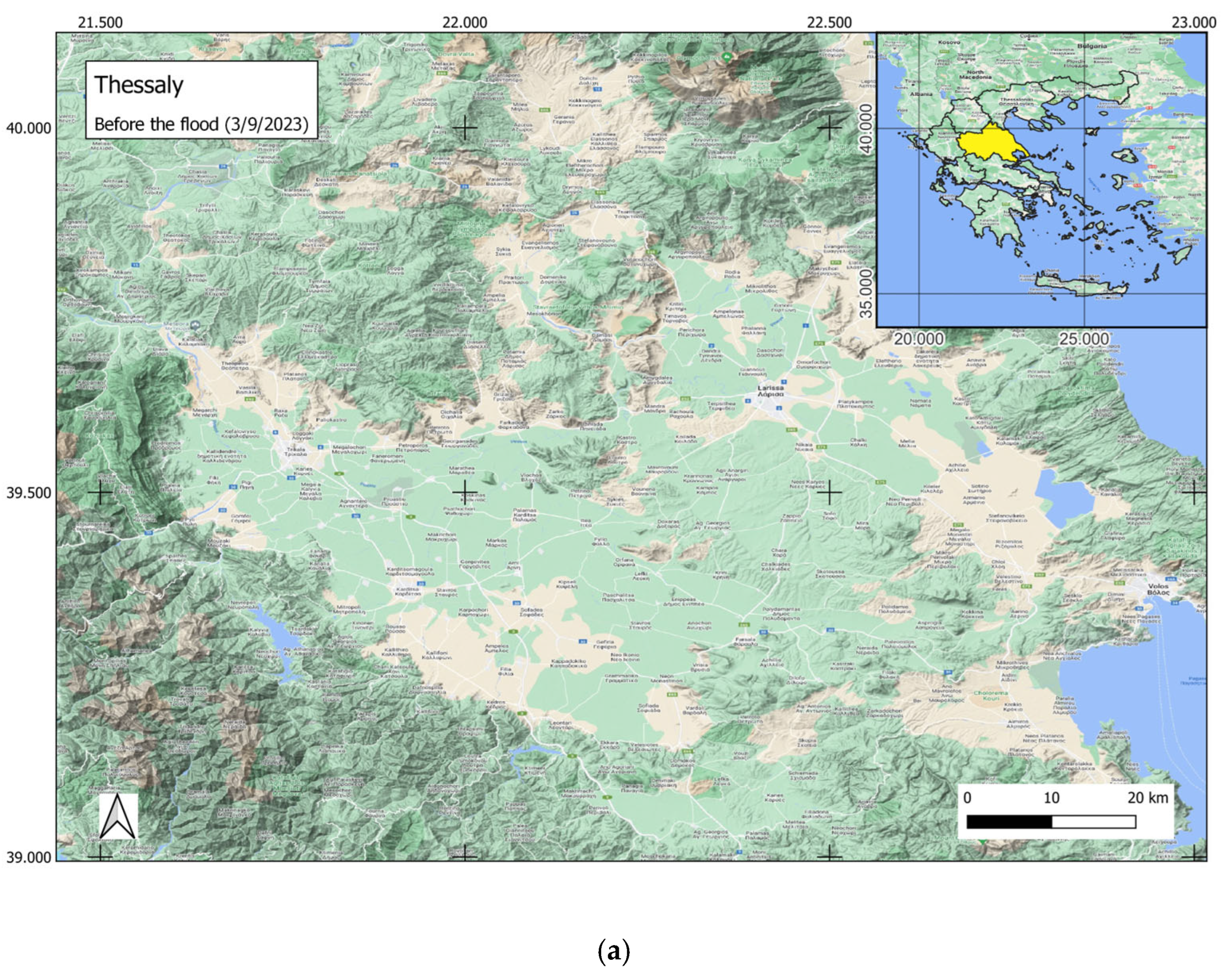
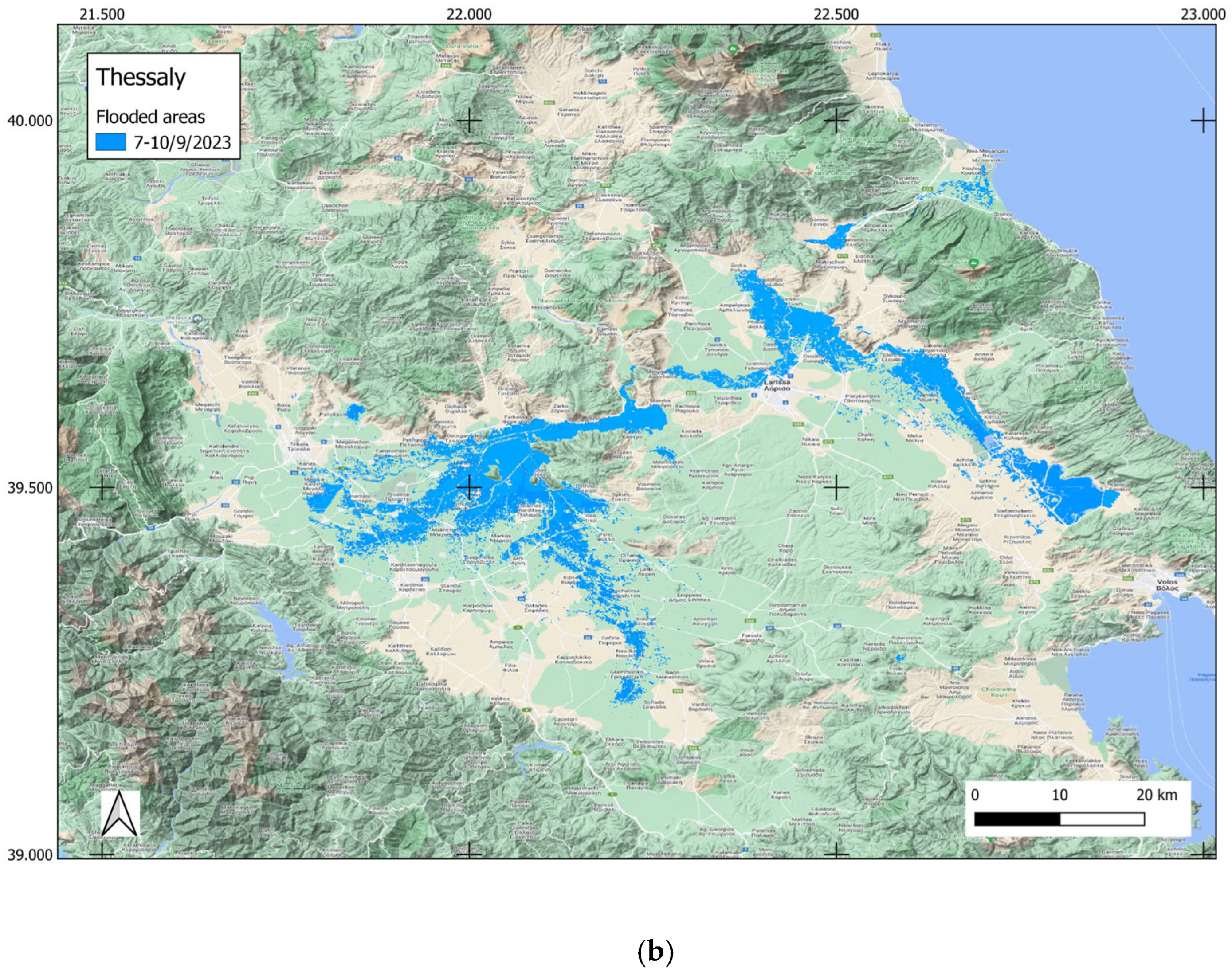
Figure 2.
Photos showing the extent of sediment accumulation following the recession of floodwaters.
Figure 2.
Photos showing the extent of sediment accumulation following the recession of floodwaters.
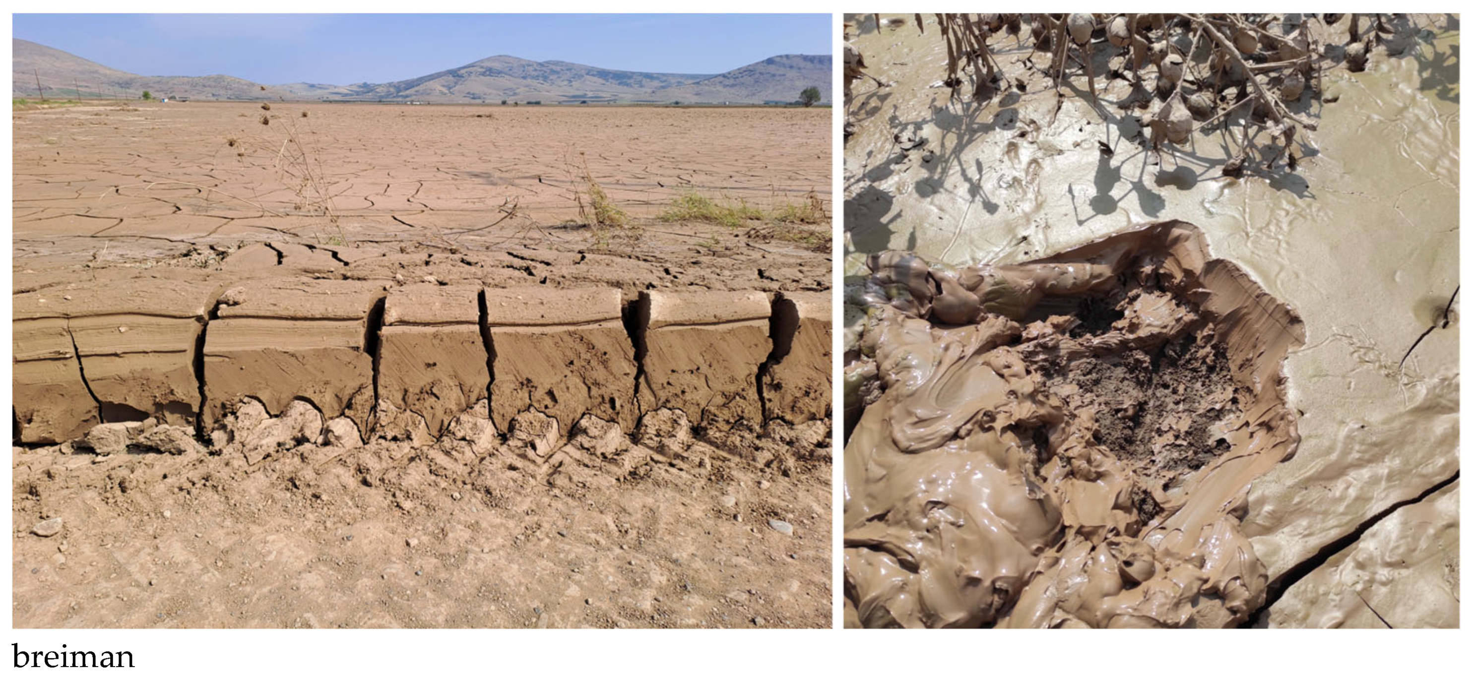
Figure 3.
The probability histograms show the distribution of Cu, Fe and Mn with zero indicating soil samples without deposit and one indicating soil samples with deposit.
Figure 3.
The probability histograms show the distribution of Cu, Fe and Mn with zero indicating soil samples without deposit and one indicating soil samples with deposit.
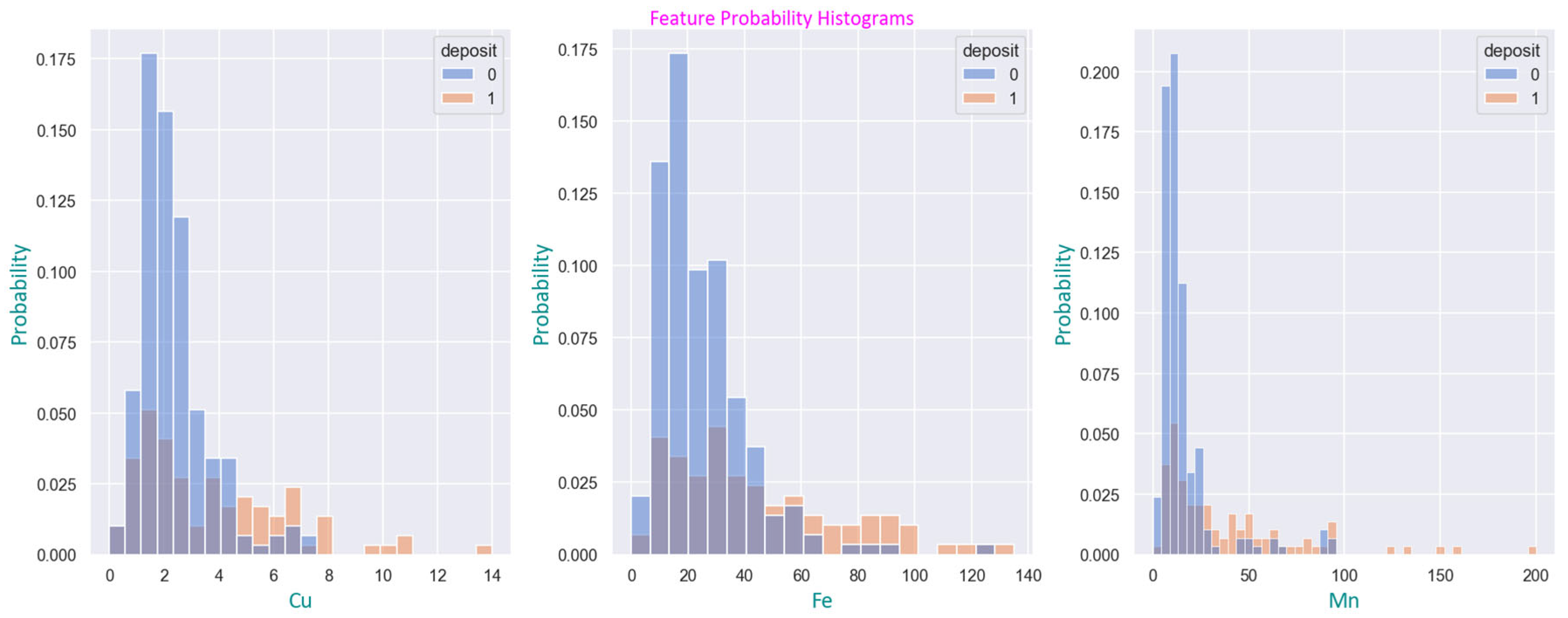
Figure 4.
Directed acyclic graph of soil variables.
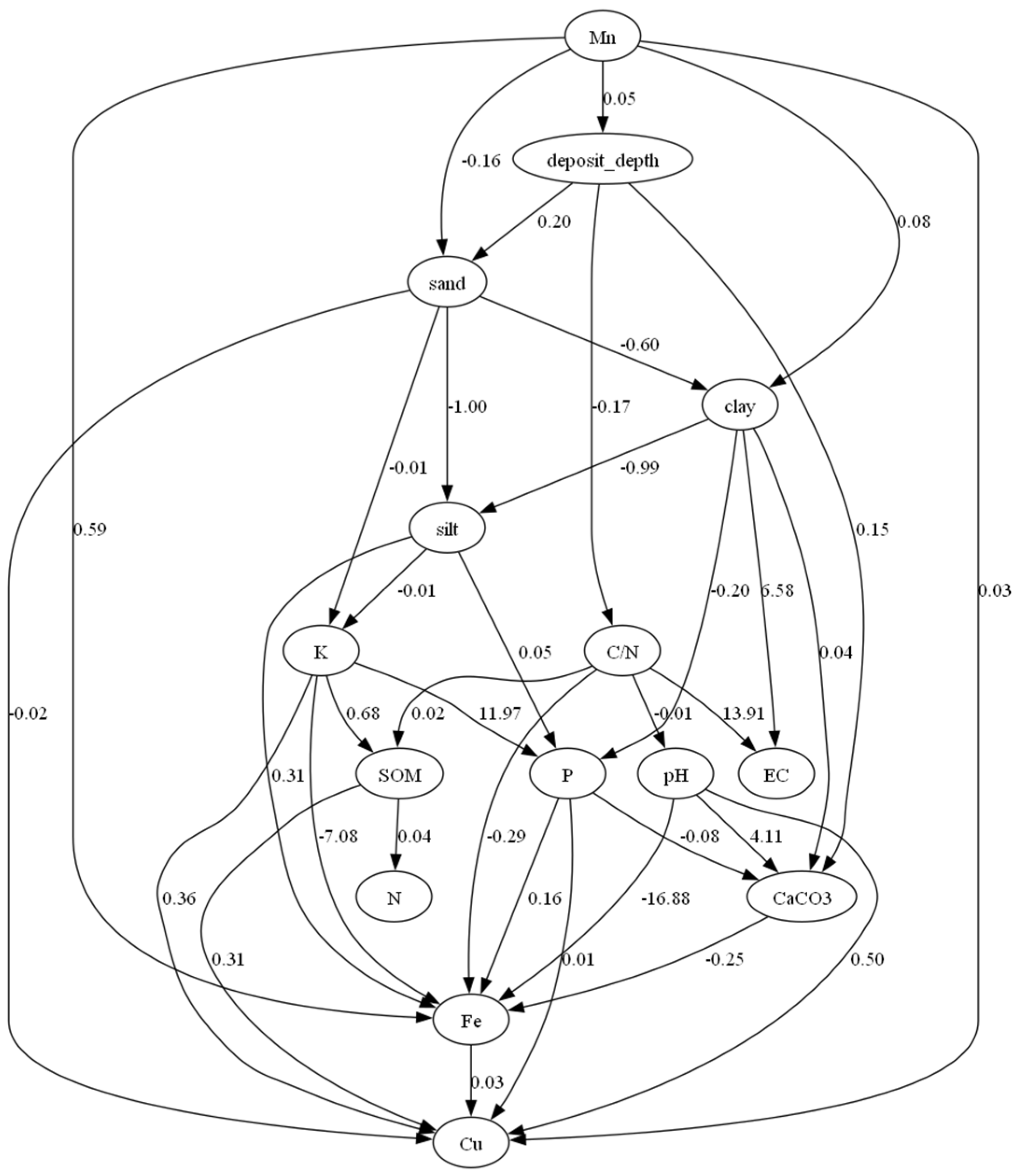
Figure 5.
Effect of deposit depth using the RESIT method on: (a) CaCO3; (b) P; (c) Mn; (d) Fe. The confidence level for the different deposit depths was obtained by bootstrapping the dataset 10 times.
Figure 5.
Effect of deposit depth using the RESIT method on: (a) CaCO3; (b) P; (c) Mn; (d) Fe. The confidence level for the different deposit depths was obtained by bootstrapping the dataset 10 times.
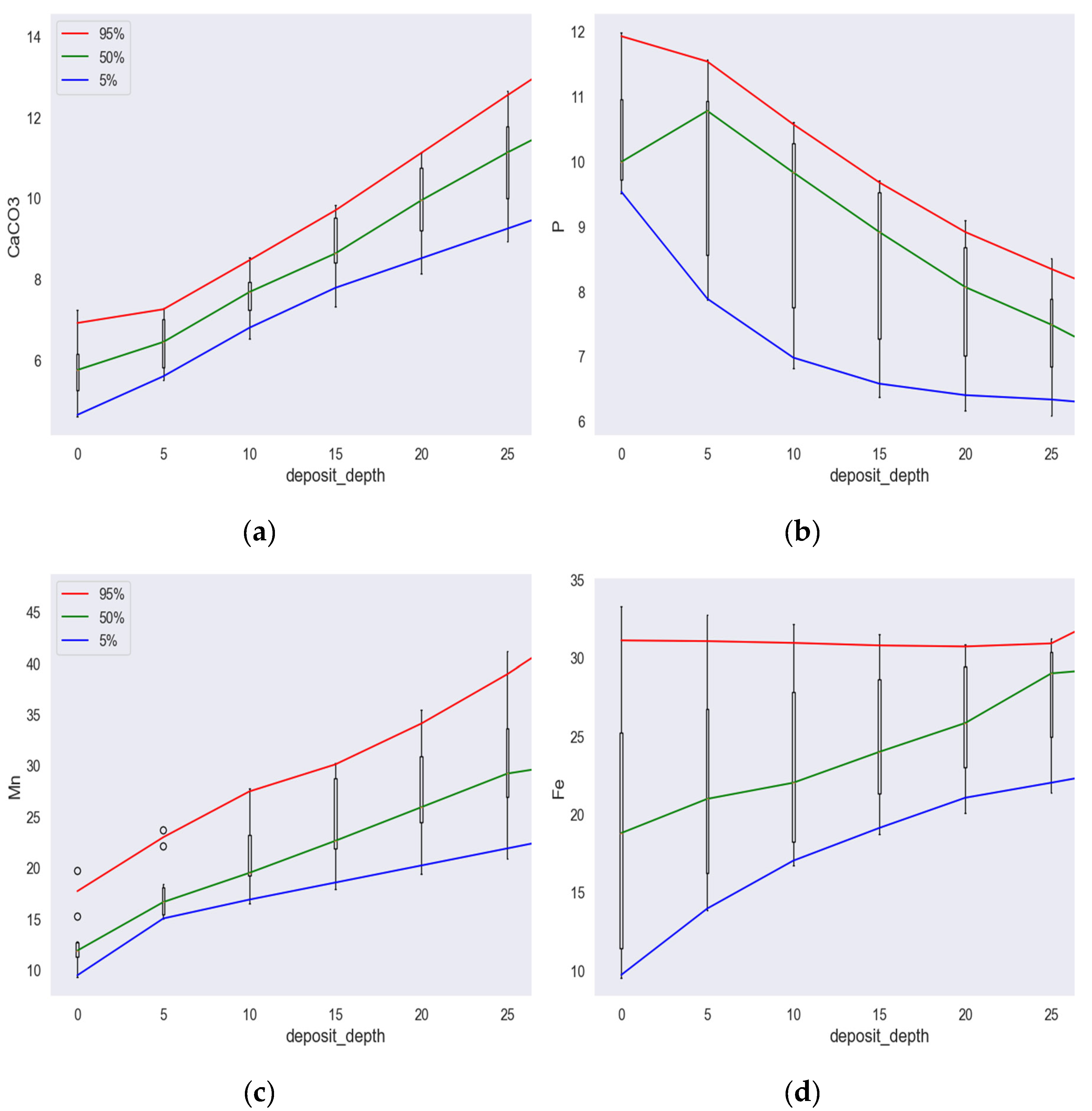
Figure 6.
Relationships of deposit depth with CaCO3, P, and Mn.
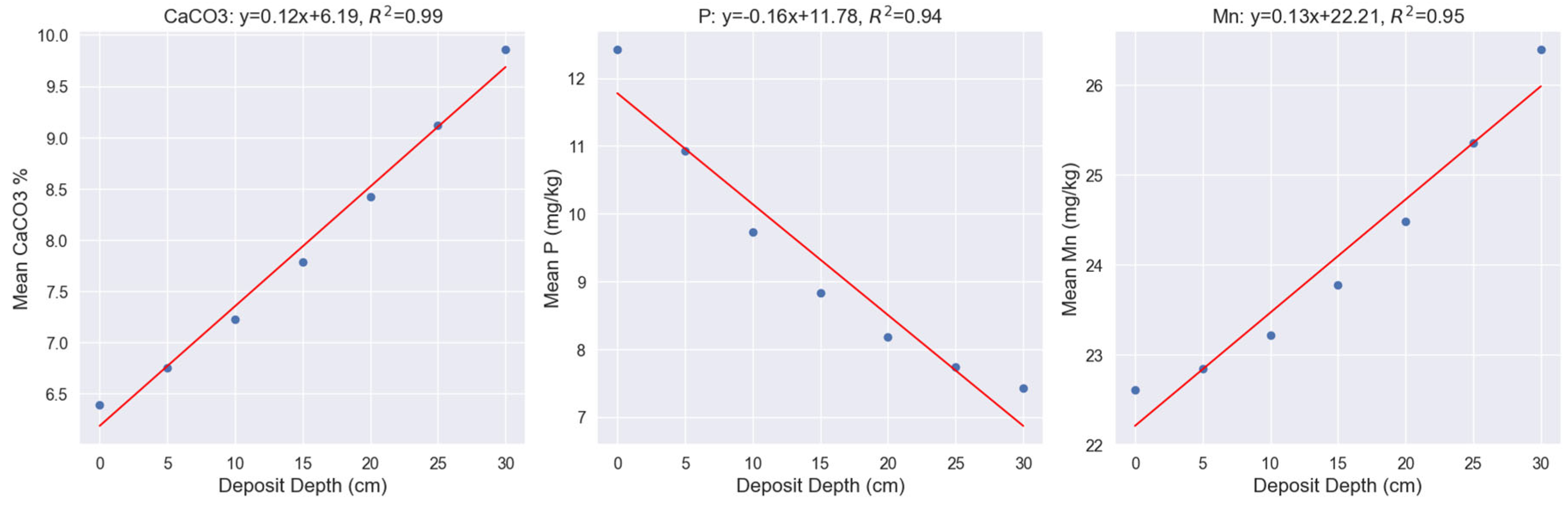
Figure 7.
The results of feature evaluation using SHAP for feature importance of LightGBM model.
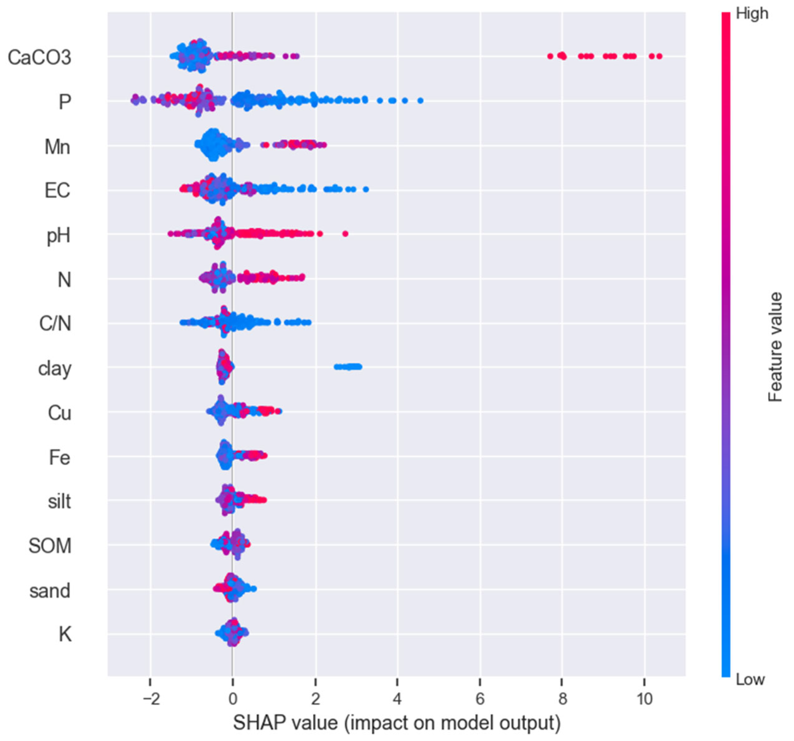
Figure 8.
SHAP dependence plots showing the interactions of: (a) CaCO3; (b) P; (c) Mn; (d) Fe.
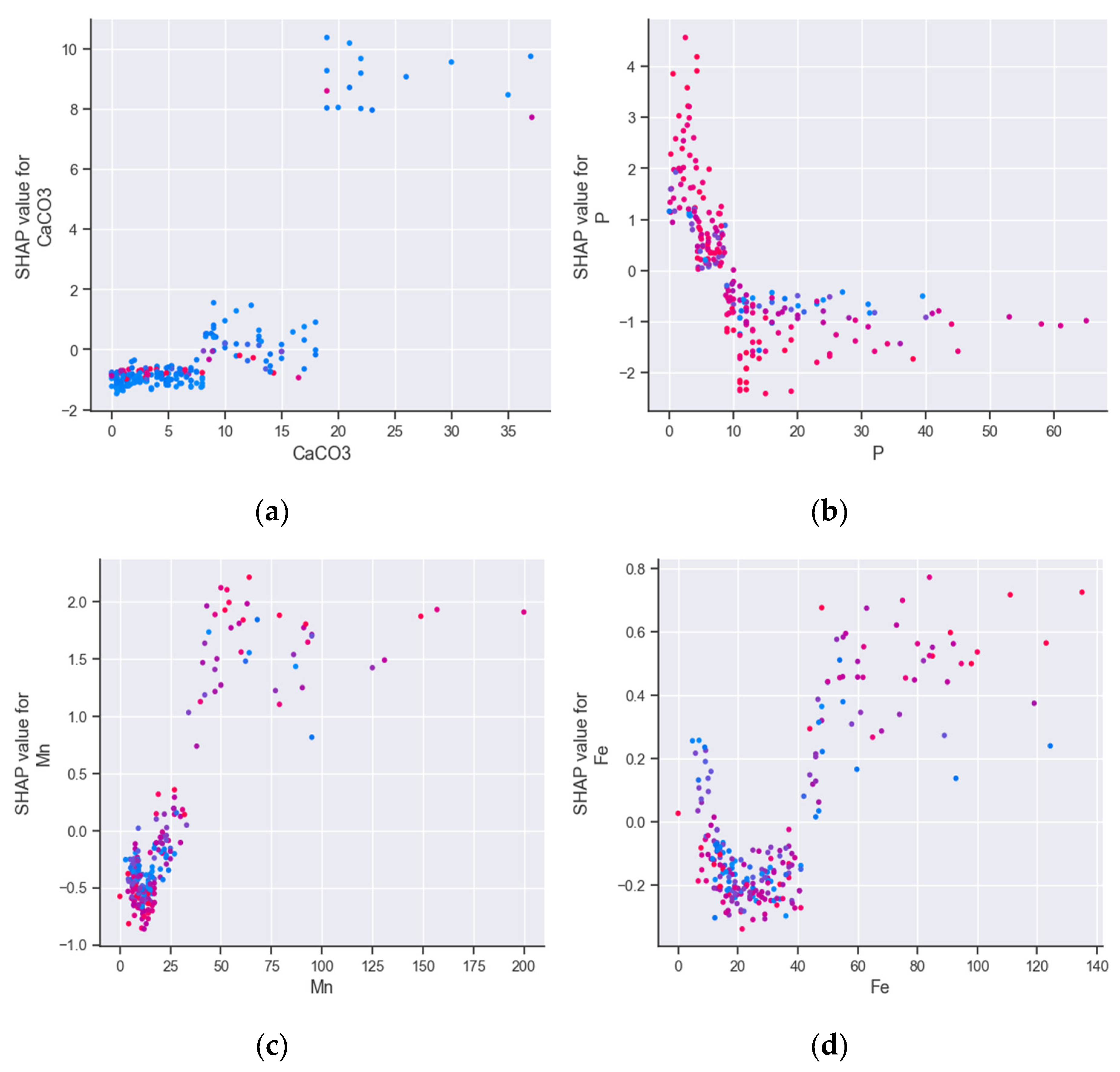
Figure 9.
Corn P fertilizer rate for deposit depth with less or more than 10 cm. Error bars display the standard error of means (s.e.m.).
Figure 9.
Corn P fertilizer rate for deposit depth with less or more than 10 cm. Error bars display the standard error of means (s.e.m.).
Disclaimer/Publisher’s Note: The statements, opinions and data contained in all publications are solely those of the individual author(s) and contributor(s) and not of MDPI and/or the editor(s). MDPI and/or the editor(s) disclaim responsibility for any injury to people or property resulting from any ideas, methods, instructions or products referred to in the content. |
© 2024 by the authors. Licensee MDPI, Basel, Switzerland. This article is an open access article distributed under the terms and conditions of the Creative Commons Attribution (CC BY) license (http://creativecommons.org/licenses/by/4.0/).
Copyright: This open access article is published under a Creative Commons CC BY 4.0 license, which permit the free download, distribution, and reuse, provided that the author and preprint are cited in any reuse.


