Submitted:
19 January 2024
Posted:
22 January 2024
Read the latest preprint version here
Abstract
The historical idea of entropy as a property of a body has been reviewed and shown to arise from Clausius’s view of heat as motion. This view of heat, being intermediate between the now defunct idea of heat as substance and the modern view that heat represents an exchange of energy, implied that a body contains a definite quantity of heat. Heat, and therefore entropy, was thus considered a property of a body. These ideas led Clausius to develop his famous inequality and the idea that entropy always increases in irreversible, non-cyclic processes. In this paper, the notion of the entropy as a property of a body is examined in detail. A physical meaning is attached to the thermodynamic entropy by showing that a change in the function Q/T can be understood as representing a change in the number of ways that energy can be distributed among the degrees of freedom active in the system at any given temperature. The idea is illustrated with reference to solids and simple liquids. It is shown that the total thermodynamic entropy is, in general, less than the Boltzmann entropy, except for the case of a monatomic classical ideal gas in which the number of degrees of freedom is independent of temperature. Finally, entropy as a state function is discussed. It is argued that this is entirely mathematical in nature and that the entropy of a state represented in p-V space is not equivalent to a physical property of a physical system in the same thermodynamic state.
Keywords:
Clausius
; Boltzmann
; thermodynamics
; entropy
; Dulong-Petit
; Debye theory
; degrees of freedom.
1. Introduction
Entropy is perhaps one of the most enigmatic concepts in physics. Whereas we can attach a clear meaning to the various forms of statistical entropy, the underlying physics of the thermodynamic entropy has presented a mystery since the foundations of the concept, with the mathematical expression for the change in the thermodynamic entropy, , affording no insight. Those properties that we do attach to the thermodynamic entropy, such as, for example, that it is an extensive property of a body that increases in irreversible processes, should more properly be considered assumptions, as there is no firm empirical evidence to support them.
Take, for example, the notion of entropy as a property of matter. The function we identify now as entropy is evident in Carnot’s analysis of a heat engine and there it is associated firmly with the transfer of heat from a reservoir. However, Carnot developed his theory using the idea of heat as caloric, the invisible, indestructible substance that was believed to permeate matter. Clausius reworked Carnot’s theory in his famous paper of 1850 [1] to take into account the then emerging idea of heat as motion. It is not commonly appreciated, however, that this was an intermediate view. It superceded the theory of caloric but came before the modern theory of heat as energy which is exchanged between bodies at different temperatures and which contributes to the total internal energy via the First law. It is this author’s belief that failure to appreciate this has led directly to a failure to appreciate the flaws in the concept of entropy.
By way of example, Tyndall [2] set out the theory of heat as motion in his book of 1865, “Heat: a mode of motion”, which was in print for over 40 years and into the 20th century in at least six editions. On page 29, Tyndall describes the effect of rapid compression of air by a piston and states that, “… heat is developed by compression of air.” The modern reader will more than likely interpret this as an old-fashioned, somewhat cumbersome way of saying that the temperature rises but this is not the meaning intended by Tyndall. On page 25, when discussing the nature of heat, Tyndall refers to two competing theories: the material view of heat as substance and the dynamical, or mechanical view in which heat is, “… a condition of matter, namely a motion of its ultimate particles”. Tyndall’s reference to heat being produced by compression should be taken literally: the kinetic energy of the constituent particles, and therefore, by Tyndall’s definition, the heat, is increased by the act of compression.
Clausius was working within the same theoretical framework. The function he later came to call the entropy of a body was derived in his Sixth Memoir, first published in 1862 [3]. It contained three variables, H, T and Z, defined as, respectively, the actual heat in a body, the absolute temperature and the disregation. Clausius claimed that H was proportional to T and may be understood as the total kinetic energy, or, according to the dynamical theory, the heat of the constituent particles. He explained the disgregation in 1866 as, “… a quantity completely determined by the actual condition of the body, and independent of the way in which the body arrived at that condition.” [4]. Neither the actual heat nor the disgregation are concepts accepted within modern thermodynamics, but Clausius’s concept of entropy is still very much accepted and it is worth considering briefly his thinking [3] in order to assess the ramifications for modern thermodynamics.
Clausius was interested in what he called, “internal work”, which is the work done on or by a particle by the inter-particle forces exerted by its neighbours. His whole purpose for developing the disgregation was to look at internal work through its effect on heat because in the mechanical theory, heat is converted to work and vice versa within the gas as a particle moves either against or in the direction of the inter-particle forces. In Clausius’s mind, this was essentially the same as the conversion of heat into so-called “external” work by a heat engine. This was summarized by a single equation which gave the sum of transformations, to use Clausius’s term, around a closed cycle of operations as:
The equality applies to reversible cycles, but in modern thermodynamics the sign of the inequality is reversed and we regard the sum as being less than or equal to zero as the modern definition of positive heat is different from that used by Clausius. He later changed his definition to accord with the modern view, but his original inequality is important because he based his thinking on that. Clausius actively sought an equivalent inequality for a single process in which heat is converted to internal work.
Clausius described the increase of disgregation as “the action by means of which heat performs work” [ref 3 , p227], and substituted the quantity TdZ for dW in what was essentially the First Law. However, TdZ also contained the internal work, but field energies were implicitly contained within the internal energy. Clausius split the latter so that a change in the internal energy was decomposed into a change in the kinetic energy, or what he called “actual heat”, and the internal work, or the field energies. As he described in 1866 [4], disgregation “serves to express the total quantity of work which heat can do when the particles of the body undergo changes of arrangement at different temperatures”. Therefore, he wrote, for reversible changes in which a quantity of heat, dQ, is exchanged with the exterior,
Notwithstanding the difficulty that one of these terms must implicitly be negative, this is essentially an expression for the conservation of energy. However, conservation of energy was not part of Clausius’s thinking. He was more concerned with reversibility and the notion of disgregation seemed to him to afford the possibility of reversible changes simply because the separation of particles could be reversed by a reverse operation. It mattered not that the process by which the separation was reversed might itself be irreversible because of his view that the disgregation represents the work that the heat can do. This led Clausius to state explicitly [ref 3, p223] that “the law does not speak of the work which heat does, but of the work which it can do.” The emphasis is Clausius’s own.
The work that heat can do is simply the reversible work, pdV, and the change TdZ therefore comprised the internal work and pdV. For an irreversible process in which dW<pdV,
This was the inequality that Clausius sought and which in his view unified cyclic and non-cyclic processes. The change in entropy of a body over a large change in volume is simply,
This is essentially the origin of the well known inequality of irreversible thermodynamics.
Three things immediately follow from Clausius’s definition of entropy in equation (4).
- H, Z and T are all properties of a body in a given state, so entropy must also be a property of a body;
- Entropy can increase through changes in H arising from internal work;
- Entropy can increase in irreversible work processes arising from changes in TdZ.
What is perhaps not so obvious is that it also violates energy conservation, as is most easily demonstrated with the free expansion. In an ideal gas there are no interparticle forces and . Equations (3) and (4) together give the change in entropy as
As T remains unchanged throughout the expansion, it follows that . This accords with the modern view. However, pdV is a work term and there is no work done in the free expansion. Neither is there any change in the internal energy, which also means that there is no heat flow. If entropy is a property of a body, then some quantity, T△S, with the units of energy is changing in a way that is inconsistent with the First Law of thermodynamics.
A similar inconsistency can be identified with the chemical potential, as described by the author in a recent conference presentation [5]. This raises the question as to whether entropy should be considered a property of a body, despite a long-standing acceptance of entropy as a property of matter within non-equilibrium thermodynamics. In that presentation, the author also presented an analysis of the entropy of a solid using silicon as an example. Looking at the entropy of a solid has the advantage that changes in volume can generally be ignored, leaving only the thermal component of entropy due to the exchange of heat. Moreover, it is the author’s experience that comparisons between the thermodynamic and statistical entropy are only ever made with reference to the classical ideal gas and solids therefore present something of a challenge.
Silicon was chosen in that presentation simply because of the author’s long familiarity with the material, but it presented a feature which contradicts the accepted picture of the thermodynamics of solids, namely that the heat capacity at high temperatures exceeds by some way 3Nk, which is the limit required by the Dulong-Petit law as well as the upper limit of the integral in the Debye theory of the specific heat. It is shown here with reference to several metals chosen at random that this is not unique to silicon and might even be a feature of the high temperature heat capacity that has not previously been considered. In addition, the theory of active degrees of freedom presented in [5] is extended to include simple liquids. However, we start this investigation of the meaning of entropy with an exploration of the chemical potential in a classical ideal gas using a geometrical interpretation. In [5], the difficulty around the chemical potential in a classical ideal gas was identified, but no solution was provided. The simplicity of the analysis afforded by the geometrical approach adopted in this paper allows a definite conclusion and implication to emerge which will be supported by the analysis of the entropy of solids.
2. The chemical potential in a classical ideal gas
Suppose we have an ideal gas containing comprising N0 particles in a volume V at temperature T0 and further suppose that we can add or extract a small number of particles, dN, such that the volume, V is allowed to change so that the system remains at the same temperature and pressure. Figure 1 shows the linear variation of U with temperature for three different values of particle number: N+>N0>N-.
As might be expected, increasing the number of particles increases U, whilst decreasing the number of particles decreases U. If particles are added, the entropy increases according to the well-known Gibbs relation,
Suppose that the system is compressed isothermally to its initial volume. The work done is pdV and the entropy decreases so that the final value for the increase in entropy caused by adding particles at the same volume is simply,
However, from Figure 1, the change in internal energy is due only to the extra particles and is:
Writing ϵ as the average energy per particle, , then,
This is problematic because the only energy change in the system is given by , so either μ=0, or μ=ϵ. These are the only two values consistent with energy conservation. Any other value implies that there is some property of the gas with the units of energy, TdS, that is changing in a way that is not consistent with the actual energy changes. It will be demonstrated that in fact, the value of μ is contrary to expectation. On the face of it, μ=0 implies that entropy doesn’t change with the addition of particles, but nonetheless a change in TdS occurs. On the other hand, μ=ϵ appears to imply that entropy changes upon the addition of particles, but TdS=0. In order to resolve this apparent paradox, the geometric analysis of Figure 1 is extended.
Entropy is usually defined to be a function of U, V and N and the chemical potential is defined by
As Figure 1 shows, however, it is not possible to change N and keep U constant without changing the temperature. Figure 2 shows the sequence of physical operations required to fulfil the conditions for the partial differential to hold.
The number of particles must be changed at constant volume and the system either cooled or heated according to whether particles are added or subtracted. Assuming particles are added, the internal energy needs to change by,
If this reduces to
In the limit , the entropy change is simply,
The entropy change can be expressed as a function of dN using equations (8) and (12):
The subscript can be dropped as this only indicates the starting state. In addition, this relationship has been derived using only the magnitudes evident in Figure 2. The requirement that U must be kept constant means that T must decrease if N is increased and vice versa. Therefore,
Writing the entropy in terms of the heat capacity, we have:
As dS is the entropy change required to maintain constant U, we can write:
Comparison with equation (10) yields,
Substitution back into equation (9) yields total entropy change of zero for the addition of particles at constant volume and temperature.
It could be argued that this assumption is implicit in the analysis. The only entropy change that has been considered is that which occurs when the system is cooled. The fact that this leads to an expression for the chemical potential that in turn confirms an entropy change of zero on the addition of particles is consistent, but not conclusive. The alternative is to put μ=0 in equation (9) and to consider the consequences. There would then be an increase in entropy of upon the addition of particles. The rest of the analysis remains the same. The system still has to be cooled to maintain constant U and this would decrease the entropy by the same amount, leading to a total entropy change of zero. From equation (10), μ=0. Again, consistent but not conclusive.
As described earlier, both of these outcomes appear to be somewhat paradoxical. On the one hand, there is no entropy is attached to the particles themselves, meaning that entropy does not increase when particles are added, yet a non-zero value of the chemical potential ensues. On the other hand, if entropy is attached to the particles and entropy increases, the chemical potential comes out as zero. However, there is no real paradox. U and N are not independent of each other and in order to maintain a constant U as N is varied means that some other operation has to be conducted. The chemical potential reflects this.
The question then arises as to which one is correct. Entropy enters thermodynamics through the flow of heat and there is no logical reason to assume it is a property of a body. However, if entropy is a property of a body, heat can be supplied at constant temperature in an isothermal expansion and its entropy correspondingly increased, but the circumstances leading to μ=0 investigated above imply an entropy of per particle in an ideal gas, which is independent of temperature. The product TS at any temperature would simply equal the internal energy, which is inconsistent with the known facts. It would mean, for example, that the Helmholtz free energy is zero. On the other hand, if no entropy is attached to the particles themselves the physical meaning of the Helmholz function is unclear, but the very fact that it can be defined and is non-zero suggests that entropy is not attached to the particles themselves.
The essential difficulty is that we do not have a microscopic understanding of thermodynamic entropy. The assumption that statistical entropy is identical to thermodynamic entropy is just that: an assumption. Although Boltzmann derived an expression for an ideal gas which was identical to the mathematical form of the thermodynamic entropy using what later came to be known as the Shannon information entropy, it is by no means clear that this mathematical identicality extends to physical equivalence or that is in fact general. In [5], the author presented an analysis of solids in which he concluded that the Boltzmann and thermodynamic entropies are not generally identical, but the analysis was restricted to a single solid, silicon. In the following, this analysis is extended to include other solids and whilst the number of materials considered is small, it shows that silicon is not unique in its properties, which contradict the known theories on the specific heat. Moreover, the analysis is extended to simple liquids arising when such solids are taken beyond their melting point.
3. Entropy in complex systems: an examination of solids
The connection between thermodynamic entropy and degrees of freedom has been established for the classical ideal gas [6] via physical interpretation of the function, , which arises because the dimensionless change in entropy at constant volume in a system with constant-volume heat capacity Cv is,
Comparison with the Boltzmann entropy, yields , which has been interpreted as the total number of ways of arranging the energy among the degrees of freedom in the system. This interpretation arises from the property of the Maxwellian distribution that it is the product of three independent Gaussian distributions of the velocity in each of the x, y and z directions. It was argued that each particle has access to, in effect, velocity states in each of the three directions, making a total of states for N particles across the three dimensions. The quantity .
The restriction to constant volume is important as it means that no energy is supplied to the system to do work and any energy that is supplied is distributed among the degrees of freedom. In a solid, the difference between the constant-volume and constant-pressure heat capacities is generally small and in practice the restriction to constant volume is not so important. Nonetheless, the change in entropy in equation (19) will still hold, but with Cv being dependent on temperature and therefore included in the integration.
The fact that the heat capacity varies with temperature means that the active degrees of freedom within the system are not so readily identifiable. In solids, it is generally accepted that the heat capacity is given by the Debye model, which accounts for a T3 dependence at low temperatures as the heat capacity tends to zero as T tends to zero. At high temperatures, the heat capacity approaches the Dulong-Petit limit of , which corresponds to six degrees of freedom per atom with the kinetic and potential energies each characterised by three degrees of freedom. As is well known, the basis of the Debye model of the heat capacity of solids is the existence of quantized vibrations and unlike a classical solid, in which the energy of the oscillation can steadily decrease simply through a reduction in the amplitude, the energy of a quantized oscillator cannot be continuously reduced. This means that at low temperatures some atoms cease to oscillate, implying that as the temperature is raised degrees of freedom are activated. However, the Debye theory of the heat capacity of a solid is not formulated in terms of degrees of freedom, but quantized oscillations and translating these into degrees of freedom is not straightforward.
The phonon spectrum of a crystalline solid always contains so-called “acoustic mode” vibrations, regardless of the solid. Despite its name, the frequency of the phonons can extend into GHz and beyond at the edge of the Brillouin zone, where the wave vector , with a being the lattice spacing. Close to the centre of the Brillouin zone the frequency tends to zero at very small wavevectors and these acoustic mode phonons represent travelling waves with relatively long wavelengths moving at the velocity of sound. These are the modes that are excited at very low temperatures and for which the solid acts as a continuum [7]. Therefore, these vibrations do not correspond to the classical picture of atoms vibrating randomly relative to their neighbours but constitute a collective motion of a large number of atoms. The average energy per atom is probably very small and it is not clear just how many effective degrees of freedom are active. By contrast, at the edge of the Brillouin zone, , meaning that the group velocity is close to, or could even be, zero. These are not travelling waves but isolated vibrations. Some materials also contain higher frequency phonon modes, called optical mode phonons because the frequency extends into the THz and beyond and the phonons themselves can be excited by optical radiation.
The detailed phonon structure for any given solid can be quite complex and the Debye theory, being general in nature, does not take this detail into account. Rather, it represents the internal energy as the integral over a continuous range of phonon frequencies with populations given by Bose-Einstein statistics and an arbitrary cut off for the upper frequency [7]. The specific heat is then derived from the variation of internal energy with temperature. Despite the wide acceptance of the Debye theory, it is also recognised that it does not constitute a complete description of the specific heats. Einstein was the first to consider the specific heat of a solid as arising from quantized oscillations, but he used a single frequency rather than a spectrum of frequencies. The transition to a continuous spectrum of phonon frequencies changed the low temperature behaviour. Instead of the T2 dependence of the specific heat derived by Einstein, Debye’s theory gives at very low temperatures. All this is well known and forms the staple of undergraduate courses in this topic, but what is perhaps not so well known is that, according the Blackman [ref 7, p24], “The experimental evidence for the existence of a T3 region is, on the whole, weak…”. Moreover, the Debye theory gives rise to a single characteristic temperature, the Debye temperature for a given solid which should define the heat capacity over the whole temperature range, but in fact does not. Low temperature heat capacities generally require a different Debye temperature from high temperature values.
This discussion of the inadequacies of the Debye model is important because in the course of this work it has become apparent that the high temperature specific heats of the solids, mainly metals, considered in this work also deviates from the expected variation and makes the association between the specific heat and the active degrees of freedom even more obscure. As discussed by Blackman [ref 7, p14], at high temperatures the Debye model should approach the classical limit of 3Nk and were it to do so the argument could be made that at any intermediate temperature the heat capacity represented the effective number of active degrees of freedom. However, in [5] the author presented data for the molar heat capacity of silicon over the whole temperature range from 0K to the melting point [8]. Close to the melting point (1687K) the constant pressure heat capacity is 28.93 J mol-1 K-1, which, assuming ½kBT per degree of freedom, is equivalent to 7 degrees of freedom per atom. Even the constant volume heat capacity, Cv, for which data is available up to 800K [9], is already 25 J mol-1 K-1 at 800K, which equates to six degrees of freedom per atom (3NAk, NA being Avogadro’s number corresponds to 24.9 J mol-1 K-1). Clearly, the heat capacity does not directly represent the active degrees of freedom because there is no classical theory which allows for 7 degrees of freedom per atom. This means that the function , which gives the number of ways of distributing the energy among the degrees of freedom in an ideal gas, has no directly comparable meaning in a solid.
Nonetheless, we can suppose that there exists at any given temperature β(T) active degrees of freedom, each associated with an average of ½kBT of energy. Then, for one mole of substance, the internal energy can be written as,
The meaning of this is perhaps not immediately apparent, but it is equivalent to taking an average heat capacity. For simplicity, let
has the units of Joules, but it can be considered a temperature if we effectively rescale the absolute temperature so that If the molar heat capacity at constant volume is , then for 1 mole,
By definition, the internal energy at some value of is,
It follows that
The angular brackets denote an average. Therefore
This is equivalent to the geometrical transformation indicated in Figure 3(a) and 3(b).
By comparison with equation (22),
By definition, for simple solids for which the heat capacity increases with temperature, , so we can expect the number of active degrees of freedom to be less than would be indicated by the heat capacity alone. Making use of equations (22) and (26) together, we have,
It follows that,
In other words, for a heat capacity that varies with temperature, the effective number of degrees of freedom is less than twice the dimensionless heat capacity, becoming equal only when all the degrees of freedom have been activated and . This is true regardless of the system, whether solid, liquid or gas. It should be noted, however, that equation (27) does not account for latent heat and therefore implies a restriction to the solid state or at least to ideal systems in which phase changes do not occur.
Figure 4(a) shows the reduced heat capacity of five solids based on the constant pressure heat capacity. As discussed in relation to equation (22), the heat capacity at constant volume should be used to give the internal energy, but it is assumed here that the difference between constant volume and constant pressure is small. Included in Figure 4(a) is data for silicon and, for comparison, germanium as a similar semiconducting material, though the available data is restricted in its temperature range [10]. The reduced heat capacity is the dimensionless heat capacity of equation (22) normalized to Avogadro’s number and a reduced heat capacity of 3 would therefore correspond to the classical Dulong-Petit limit of a molar heat capacity of 3NAk. In all cases, the reduced heat capacity exceeds 3 at a temperature close to the Debye temperature. Figure 4(b) shows the mean reduced heat capacity of four of the solids for which data down to T=0 is readily available.
There is nothing particular about the elements represented in Figure 4 other than that they have moderate to low melting points. They were otherwise chosen because an internet search produced a complete range of data for each of the three metals, aluminium [11], indium [12] and lead [13]. It is noticeable that, with the exception of lead, all four have a mean reduced heat capacity below three. Even for lead, the discrepancy is less than 3%, with the maximum value being 3.08. Arblaster claims an accuracy of 0.1% in his data for temperatures exceeding 210K [13], but it should be noted that in all cases in Figure 4(a), the heat capacity relates to constant pressure rather than constant volume. Strictly, the latter is required to calculate the internal energy and hence the mean heat capacity, but, experimentally, measurement at constant pressure is much easier to undertake. Transformation to constant volume is straightforward given knowledge of the compressibility as well as the thermal expansivity [7] and reduces the heat capacity slightly, but without doing the calculations it is not possible to say for certain that the mean reduced heat capacity at constant volume will stay below 3.
Figure 4(a) shows very clearly, however, that the heat capacity is not a direct representation of the active degrees of freedom. By definition, from equations (20) and (26), the mean heat capacity is a direct representation of the number of effective degrees of freedom and it is clear that even up to the melting point, the small excess with lead notwithstanding, there are less than 3kT associated with each constituent atom.
The mean heat capacity can now be used to attach a physical meaning to the thermodynamic entropy. From equation (20), the change in internal energy is
Under the assumption that the internal energy is partitioned equally among active degrees of freedom, the change in internal energy comprises two components: the change in the average energy among the degrees of freedom already activated and the distribution of some energy into newly activated degrees of freedom, each of which contains an average energy . Both of these terms contribute to the entropy. However, as the change in internal energy is written in terms of TB, it is necessary to divide the entropy by kB to give the dimensionless quantity,
Upon substitution of equation (29), the dimensionless entropy change is,
Here we make use of the fact that
It is notable that the entropy is still given as a function of the absolute temperature in Kelvins and the reason for this will become clear.
The first term on the right in equation (31) can be interpreted as the change in the function , which has already been defined for a classical ideal gas as the number of arrangements by direct comparison of the thermodynamic entropy and Boltzmann’s entropy [6]. Straightforward differentiation of lnW with respect to lnT yields
The change in thermodynamic entropy therefore represents the fractional change in the number of arrangements or, equivalently, the change in the Boltzmann entropy, plus the addition of new degrees of freedom. Integrating equation (31) by parts to get the total entropy at some temperature T1, we find,
At , , but and the lower limit is also zero. Therefore,
The first term on the RHS is recognizable as the Boltzmann entropy, . In the second term on the RHS, is a positive number for T>1, and greater than unity for . Therefore, for systems in which the heat capacity varies with temperature the thermodynamic entropy at any given temperature above approximately 3K is less than the Boltzmann entropy for the simple reason that the number of arrangements at any given temperature depends only on the number of degrees of freedom active at that temperature, whereas the thermodynamic entropy, being given by an integral over all temperature, accounts for the fact that the number of degrees of freedom have changed over the temperature range. This relationship is illustrated in Figure 5.
4. Extension to simple liquids and gases
The preceding treatment can be generalized by writing the internal energy as,
Rearranging slightly,
The average heat capacity over the temperature range TB1 to TB2 can be defined by dividing through by the temperature difference,
This gives the change in internal energy as,
Rewriting,
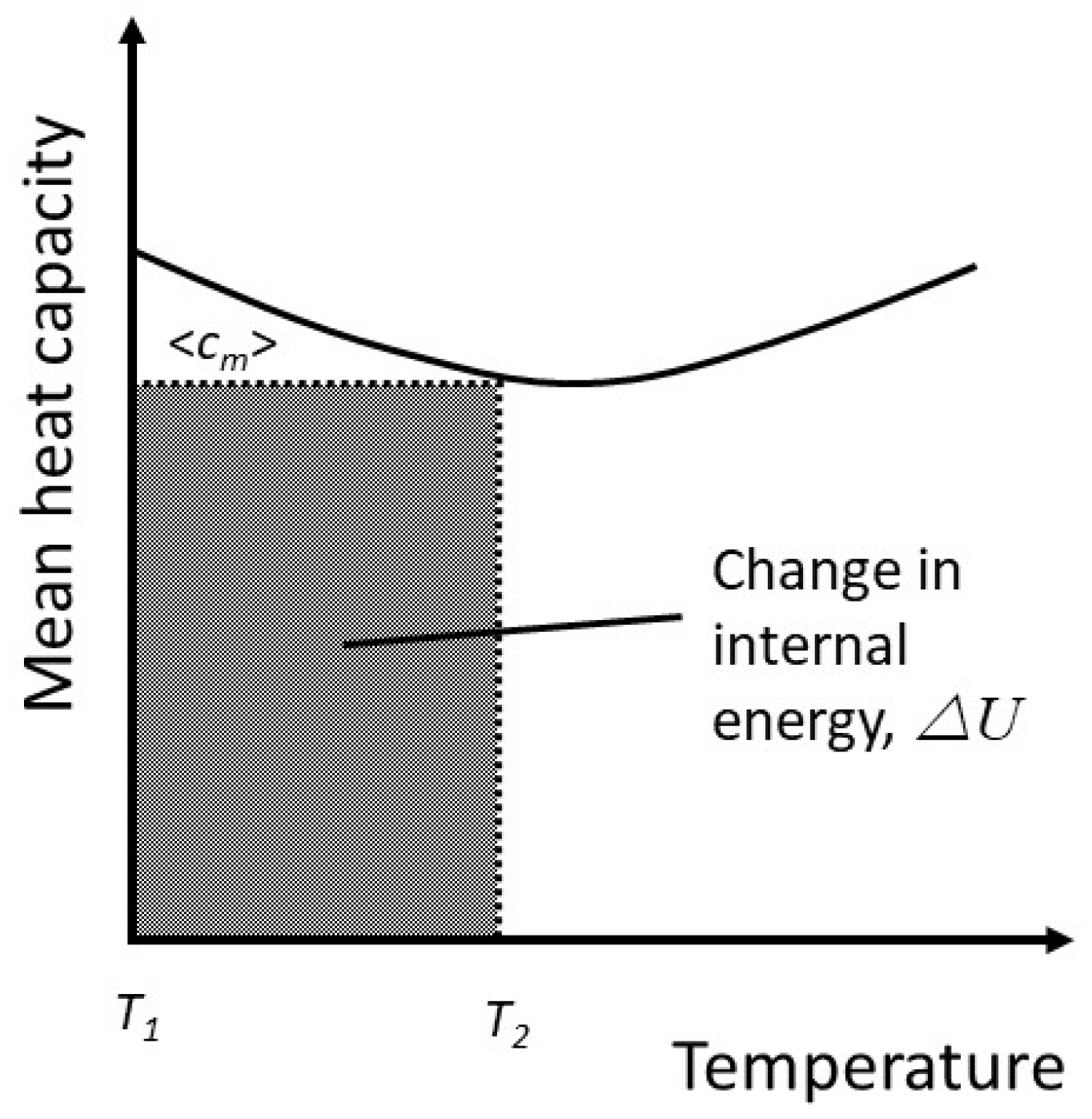
If TB1=0, △U=U and △TB=TB, recovering the preceding formulation. The similarity is revealed by a similar geometric interpretation to Figure 3(b), as shown in Figure 6.
The advantage of this approach is that it allows for phase changes by looking only at the change in the internal energy within, say, the liquid phase, or the vapour phase. By way of example, consider lead vapour. Arblaster [13] gives the constant pressure heat capacity of lead as a function of temperature for all phases: solid, liquid and both monatomic and diatomic vapour. The data for vapour covers the temperature range from well below melting, 298.15K, to well above boiling, 2400 K. The monatomic vapour has a heat capacity of 20.786, corresponding to 3 degrees of freedom, up to approximately 700K, whereupon it begins to increase steadily, reaching 28.174 at 2400K. Quite clearly, the vapour over the solid is acting like an ideal gas. Whatever degrees of freedom characterized the atoms as part of a solid and whatever energy has been absorbed in order to liberate the atoms from the solid are irrelevant to both the degrees of freedom and the kinetic energy in the vapour phase, the latter being simply the thermal energy.
Suppose we have 1 mole of vapour which has been created at some temperature TB1. Expanding equation (40), and substituting , we would have, at some higher temperature TB,
This admits to a simple physical interpretation. is the total energy supplied to create the vapour, which has an effective thermal energy at this temperature and is the effective thermal energy at TB. Unlike the case of a solid, in which is directly related to the number of active degrees of freedom via equation (26), it is not so obvious that for either a vapour or a liquid, the mean dimensionless heat capacity has the same physical interpretation. However, it has been argued that the active number of degrees of freedom following a phase change is entirely independent of the number of degrees of freedom preceding the phase change, and if, say, a vapour were to behave like an ideal gas with a constant heat capacity between the vapourisation point and some arbitrary higher temperature, then averaged over that temperature range would be exactly equal to half the number of degrees of freedom. It follows that, in general, if the heat capacity varies with temperature must represent some quantity that reduces to in this limiting case and it seems reasonable to assume that equation (26) holds in this case also. It would also be reasonable to assume that the same applies to a liquid, not least because the internal energy can effectively be expressed as a function of absolute temperature via equation (41).
The change in entropy can be derived from equation (41) as,
The last term on the right is recognizable as the change in the Boltzmann entropy and the first termon the right tends to as TB increases. For equation (42) reduces to equation (31). It follows from the preceding argument that the total entropy change in either the liquid or vapour phase will be less than the Boltzmann entropy at the higher temperature for positive changes in β. If β decreases, as illustrated in Figure 6, the thermodynamic entropy might well exceed the Boltzmann entropy.
5. Discussion and conclusion
This paper opened with a historical analysis of the development of the concept of entropy by Clausius and showed how his ideas violate energy conservation for irreversible processes. There was, nonetheless, a compelling logic to his arguments. The belief that heat was a property of a body meant that some property of the body must have changed during an isothermal expansion. As the internal energy remains unchanged, and in an ideal gas this was equivalent to Clausius’s idea of the heat content, it followed that the change must be bound up with the separation of the particles. In a real gas subject to inter-particle forces, a change in volume will affect the potential energy of the particles and with it the kinetic energy, or heat as understood by Clausius. However, heat is no longer defined as motion and therefore no longer regarded as a property of a body. Instead, it represents an exchange of energy, but the concept of entropy was not revised in the light of this change. Logically, entropy, , should more properly be associated with a transfer of heat, δQ.
It has been shown that applying this constraint to the entropy change consequent upon the addition of particles to an ideal gas leads to a non-zero value of the chemical potential owing to the fact that an exchange of energy with the exterior must occur in order to maintain a constant internal energy within the system, but this example also illustrates one of the difficulties in interpreting the concept of entropy. It is a derived quantity which is not susceptible to empirical observation and mathematical consistency is not sufficient. In this analysis of the chemical potential, a different assumption about the energy attached to particles leads to a different value of the chemical potential which is consistent with the initial assumption. In order to decide which is correct, it is necessary to go beyond these arguments and look at the wider picture. In this paper, this has been attempted by trying to attach a physical meaning to the change in entropy of a solid. This follows work by the author in 2008 [6] that showed that the apparent entropy of a classical ideal gas can be described by the distribution of energy over the available states, which were defined to be per degree of freedom.
This arises from the normal distribution of energy within each classical degree of freedom, whether related to kinetic or potential energy. The variance is related to the thermal energy and depends on T, meaning that the standard deviation, and with it the width of the distribution, depends on . In this paper, the temperature has effectively been rescaled and in this view the number of states depends on . The spacing between states then varies with for velocity states. Were the same reasoning to be applied to systems which oscillate harmonically, the spacing between states would be , where keff is the effective spring constant.
In principle, this should allow the theory to be applied to solids. Even though the heat capacity is derived from quantized oscillations, it is generally assumed that this is equivalent in the high temperature limit to the classical picture and that the number of degrees of freedom is given by the Dulong-Petit law. The present work has shown that this is not the case for many materials and that the heat capacity exceeds 3Nk at well below room temperature in the case of low melting point materials like lead and indium. This would seem to preclude additional contributions from electrons to the specific heat, but without detailed calculations this cannot be stated for certain.
Although the specific heats of only 5 solids are shown in Figure 4, these have been chosen at random and there is no reason to suppose that most simple solids do not behave in this way. It would seem from this that neither the Dulong-Petit law nor the Debye model of specific heats are effective, but it is possible to define the effective number of degrees of freedom as the mean heat capacity taken over the temperature 0K to the temperature of interest. It appears that the number of effective degrees of freedom is less than six, but further work is required to establish just how general this is. Were it to prove to be general, it would be an obvious modification to the Dulong-Petit law to express this as the high temperature limit, but that would still require some revision of the Debye model, as 3Nk is assumed to be the high temperature heat capacity.
Having defined the effective number of degrees of freedom, the change in thermodynamic entropy upon constant volume heating has been shown to be directly related to the change in the number of ways of distributing the increased internal energy among the active degrees of freedom. This then brings the interpretation of the thermodynamic entropy in solids in line with the interpretation for the classical ideal gas. It has been shown in consequence that the total thermodynamic entropy of a solid at any given temperature is less than the corresponding Boltzmann entropy, which gives only the number of ways of distributing energy among the existing degrees of freedom and takes no account of the thermal history. The treatment has been extended to include phase changes from liquid to solid and again the argument is made that the thermodynamic entropy of a liquid at any given temperature is different from the Boltzmann entropy. It might even exceed the Boltzmann entropy as the effective number of degrees of freedom will decrease with temperature in line with a decrease in the heat capacity, which is very common in simple liquids [14].
Finally, some comment about the connection between the thermodynamic entropy and the Shannon information entropy is in order. The Boltzmann entropy is a special case of the Shannon information entropy in the case of a uniform probability distribution for the access to each state. In the case of a classical ideal gas, the Shannon entropy of the Maxwellian distribution agrees with the apparent thermodynamic entropy and in turn the Boltzmann entropy. In the case of a solid, this author is not aware of any paper that sets out a distribution over phase for the particles, as the existing Debye theory of specific heat and internal energy is based on an entirely different set of concepts. Even if it were possible to express the probability of an individual particle having a velocity in an interval v to v+dv or a displacement from some central position in the range r to r+dr, these would at best agree with the Boltzmann entropy. The essential difficulty revealed in this paper would remain: that the thermodynamic entropy and statistical entropies are not the same thing and it is the change in thermodynamic entropy that has a statistical interpretation: it relates to the change in the distribution of energy over the available degrees of freedom.
This leaves the ideal classical gas as a special case. The thermodynamic and statistical entropies are the same because the specific heat is independent of temperature. That does not mean to say, however, that the thermodynamic and statistical entropies are physically equivalent. This paper has focused solely on the effect of changing the internal energy, but in a gas changes in entropy can arise from work. The mathematical equivalence of the statistical and thermodynamic entropies does not reflect the fact that in an isothermal expansion, which is itself an unattainable ideal, heat flows into a system to maintain the internal energy but in the statistical interpretation, the volume dependence arises because the particles have access to a greater volume and hence require a different probability distribution to describe their positions. The statistical entropy is therefore a property of the state of the gas whereas the thermodynamic entropy is not. It is precisely the association of thermodynamic entropy with both volume and the number of particles in a system that leads to the conflict with the First Law, as demonstrated via the examples presented in this paper.
The obvious response to this is that entropy is a state function, but this is a mathematical property of thermodynamic phase space. It arises purely from the differential geometry of ideal trajectories between states represented in phase space. The trajectories are ideal because every state is accessible from any other state by any number of paths. By definition, such trajectories are not only reversible in themselves, but also allow for reversible cyclic processes. The entropy thus defined represents the heat that would have to be supplied in order to execute any one of these ideal trajectories. This is purely mathematical. Real physical processes are unlikely to be reversible [15] and such trajectories may not be realisable by real physical processes. The idea of entropy as a state function does not require the entropy to be a physical property of a thermodynamic system in a given thermodynamic state. It is simply a mathematical property of the differential geometry of the ideal trajectories.
This comes right back to Clausius’s view, described at the beginning of this section, that entropy is bound up with the separation of particles. An ideal trajectory is comprised of reversible adiabatic and isothermal transitions between states. Entropy changes only on the isothermal elements, but as the internal energy remains unchanged, the distribution of energy among the available degrees of freedom is also unchanged. For the entropy to be a property of the gas which increases in an isothermal work process, it must be connected to the volume available to the particles. This would imply in turn that entropy has to increase in an irreversible process, which has the effect of separating entropy from the exchange of heat and conflicts with the First Law.
In conclusion, it has been argued that the notion that entropy is a property of a body derives from Clausius’s conception of heat as a property of a body and that, logically, it should be associated with an exchange of heat. It has been argued in consequence that:
- the total thermodynamic entropy has no physical meaning, but that the change in entropy associated with a change in internal energy can be understood as being comprised of a change in the distribution of energy among the degrees of freedom as well as the activation of new degrees of freedom where relevant;
- the notion of entropy as a state function does not, and should not, imply that entropy is a property of a body in a given thermodynamic state. Rather, it arises from the differential geometry of thermodynamic phase space.
Funding
This research has been conducted by the author independently and without any funding from any organisation.
Conflict of interest
The author declares no conflicts of interest in the preparation or publication of this manuscript.
References
- Clausius, R. 1867. On The Moving Force Of Heat And The Laws Of Heat Which May Be Deduced Therefrom, in The Mechanical Theory of Heat, with its applications to the steam engine and to the physical properties of bodies, Ed. T. Archer Hirst, John van Voorst, London, pp14-69.
- Originally published in 1863, a reprinted version is available at: Tyndall, J. 2014. Heat Considered as a Mode of Motion: Being a Course of Twelve Lectures Delivered at the Royal Institution of Great Britain in the Season of 1862, Cambridge University Press, ISBN 9781107239449. [CrossRef]
- Clausius, R. 1867. On The Application Of The Equivalence Of Transformations To Interior Work, in The Mechanical Theory of Heat, with its applications to the steam engine and to the physical properties of bodies, Ed. T. Archer Hirst, John van Voorst, London, pp215-250.
- Clausius, R. 1866. On the determination of the Disgregation of a Body and on the True Capacity For Heat, Phil. Mag. 31 28-22, p29.
- Sands, D 2022. The Problem of Entropy in the Teaching of Thermodynamics, presented at the International Conference FFP16, Istanbul, May 23-26, 2022, Proceedings to be presented in the book series: Springer Proceedings in Physics (SPPHY, volume 392). [CrossRef]
- Sands D. 2007. Thermodynamic entropy and the accessible states of some simple systems. European Journal of Physics.;29(1):129-135.
- Blackman, M. 1941. The Theory Of The Specific Heat Of Solids, Rep. Prog. Phys. 8 11.
- Desai, P. 1986. Thermodynamic Properties of Iron and Silicon. Journal of Physical and Chemical Reference Data 15(3):967-983.
- Wei S, Li C, Chou M. 1994. Ab initio calculation of thermodynamic properties of silicon. Physical Review B. 50(19):14587-14590.
- Crouch, R.K., Fripp, A.L., Debnam, W.J.; Taylor, R.E. and Groot, H. 1981. Thermophysical Properties of Germanium for Thermal Analysis of Growth From the Melt. MRS Online Proceedings Library 9, 657–663. [CrossRef]
- Kozyrev, Nikolay V., and Vladimir V. Gordeev. 2022. "Thermodynamic Properties and Equation of State for Solid and Liquid Aluminum" Metals 12, no. 8: 1346. [CrossRef]
- Khvan, A.V.; Konstantinova, N.; Uspenskaya, I.A.; Dinsdale, A.T.; Druzhinina, A.I.; Ivanov, A. and Bajenova, I. 2022. A description of the thermodynamic properties of pure indium in the solid and liquid states from 0 K, Calphad, 79, 102484, ISSN 0364-5916. [CrossRef]
- Arblaster, J.W. 2012. Thermodynamic properties of lead, Calphad, 39, 47-53, ISSN 0364-5916. [CrossRef]
- Schirmacher, Walter; Bryk, Taras and Ruocco, Giancarlo, 2022. Comment on “Explaining the specific heat of liquids based on instantaneous normal modes”, Phys. Rev. E 106, 066101. [CrossRef]
- Norton, J. D. The Impossible Process: Thermodynamic Reversibility, Studies In History and Philosophy of Science Part B Studies In History and Philosophy of Modern Physics 55, T: Impossible Process. [CrossRef]
Figure 1.
The dependence of internal energy on temperature for a classical ideal gas. Three different particle numbers are illustrated, with N+>N0>N-.
Figure 1.
The dependence of internal energy on temperature for a classical ideal gas. Three different particle numbers are illustrated, with N+>N0>N-.
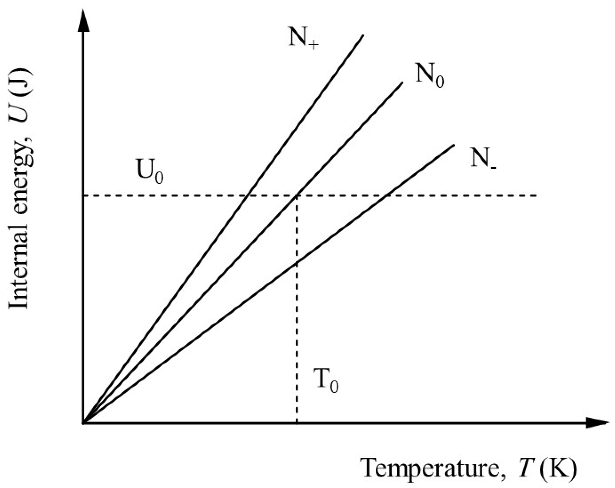
Figure 2.
The sequence of operations required to maintain constant internal energy. Particles can be added or subtracted at constant temperature, thereby changing the internal energy (a), so the system has to be either cooled or heated to restore the internal energy to its initial value (b).
Figure 2.
The sequence of operations required to maintain constant internal energy. Particles can be added or subtracted at constant temperature, thereby changing the internal energy (a), so the system has to be either cooled or heated to restore the internal energy to its initial value (b).
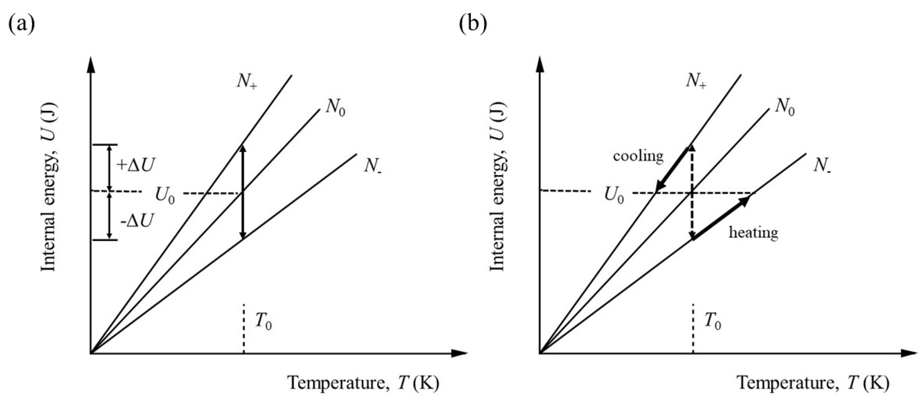
Figure 3.
A schematic representation of the change in geometric interpretation of the internal energy from an area under a curve (a), corresponding to equation (23), to the area of a simple rectangle (b), corresponding to equation (25).
Figure 3.
A schematic representation of the change in geometric interpretation of the internal energy from an area under a curve (a), corresponding to equation (23), to the area of a simple rectangle (b), corresponding to equation (25).
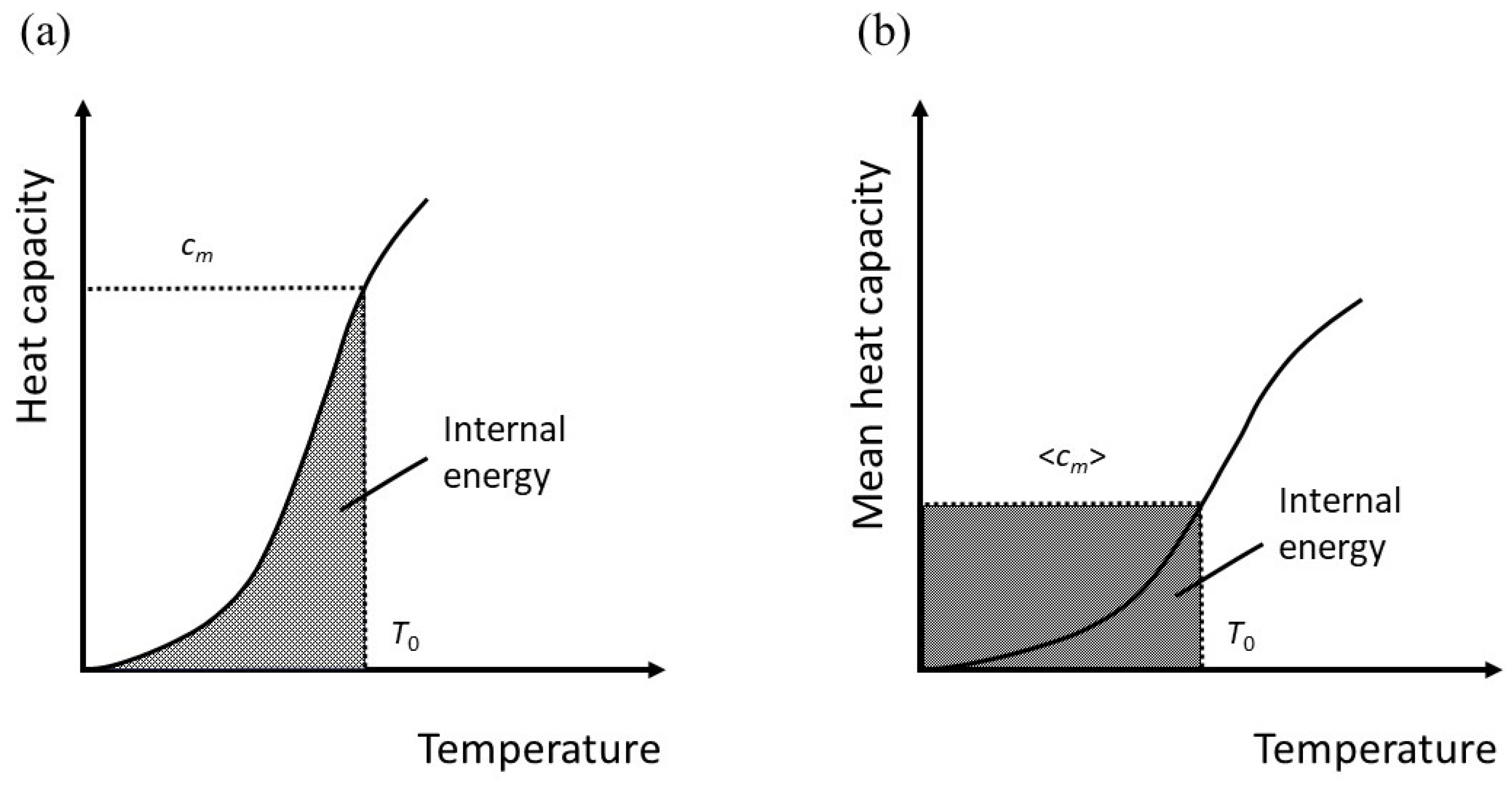
Figure 4.
The specific heat of three different metals, In [12], Al [11], Pb[13] and Si [8] from 0K to their respective melting points. The specific heat of Ge [10] is shown over a limited range of temperature range, but including the melting point, for direct comparison with silicon. Figure 4b shows the means reduced heat capacity, which is effectively half the number of active degrees freedom per atom, for each of the materials in (a).
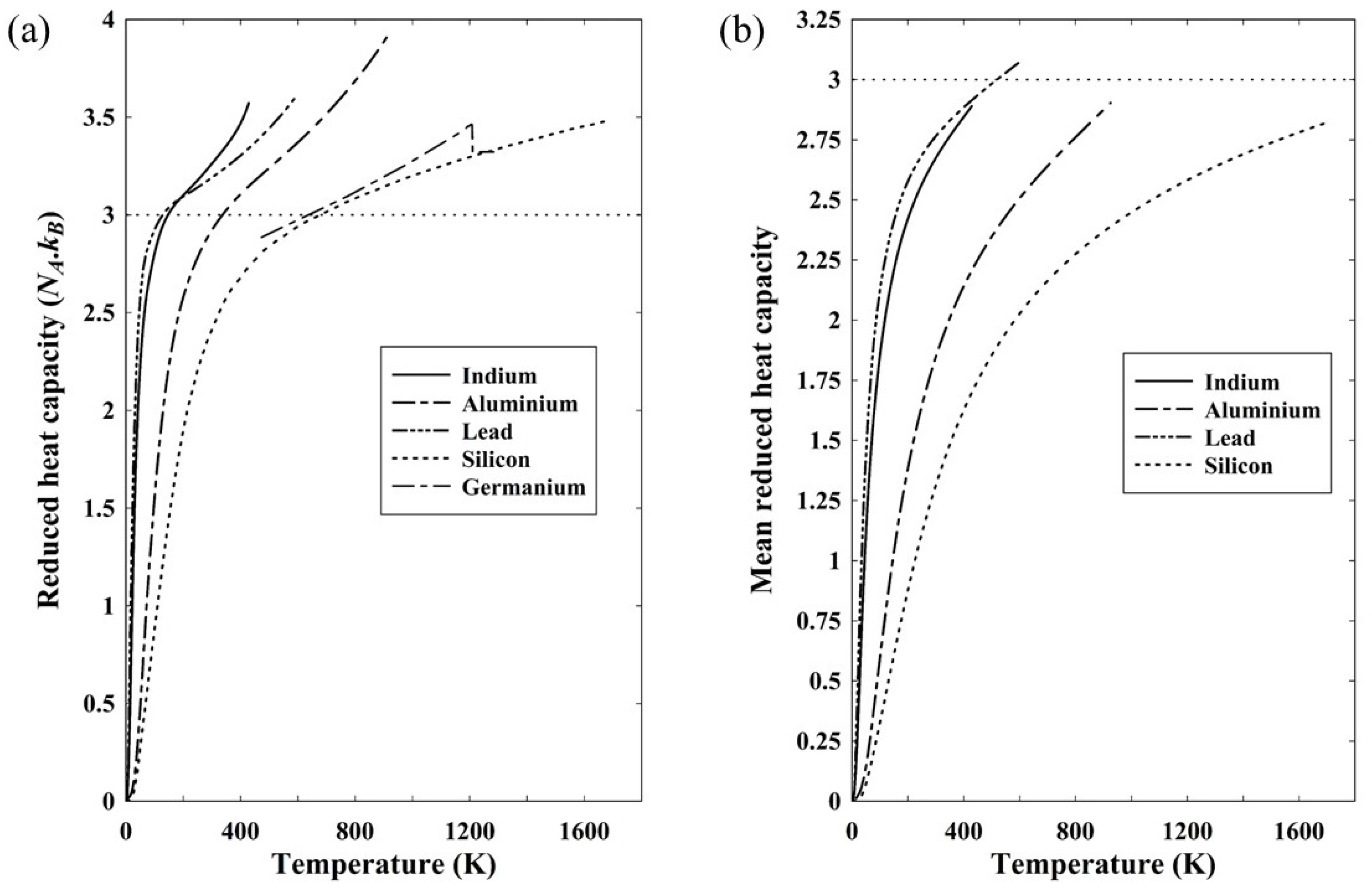
Figure 5.
A geometric representation of equation (35), with . The Boltzmann entropy is simply the area of the rectangle defined by the value of at any given value of except for a very small contribution corresponding to T<1, or ln T <0. The thermodynamic entropy is given by the unshaded area and is seen to be equal to the Boltzmann entropy when ln T=1.
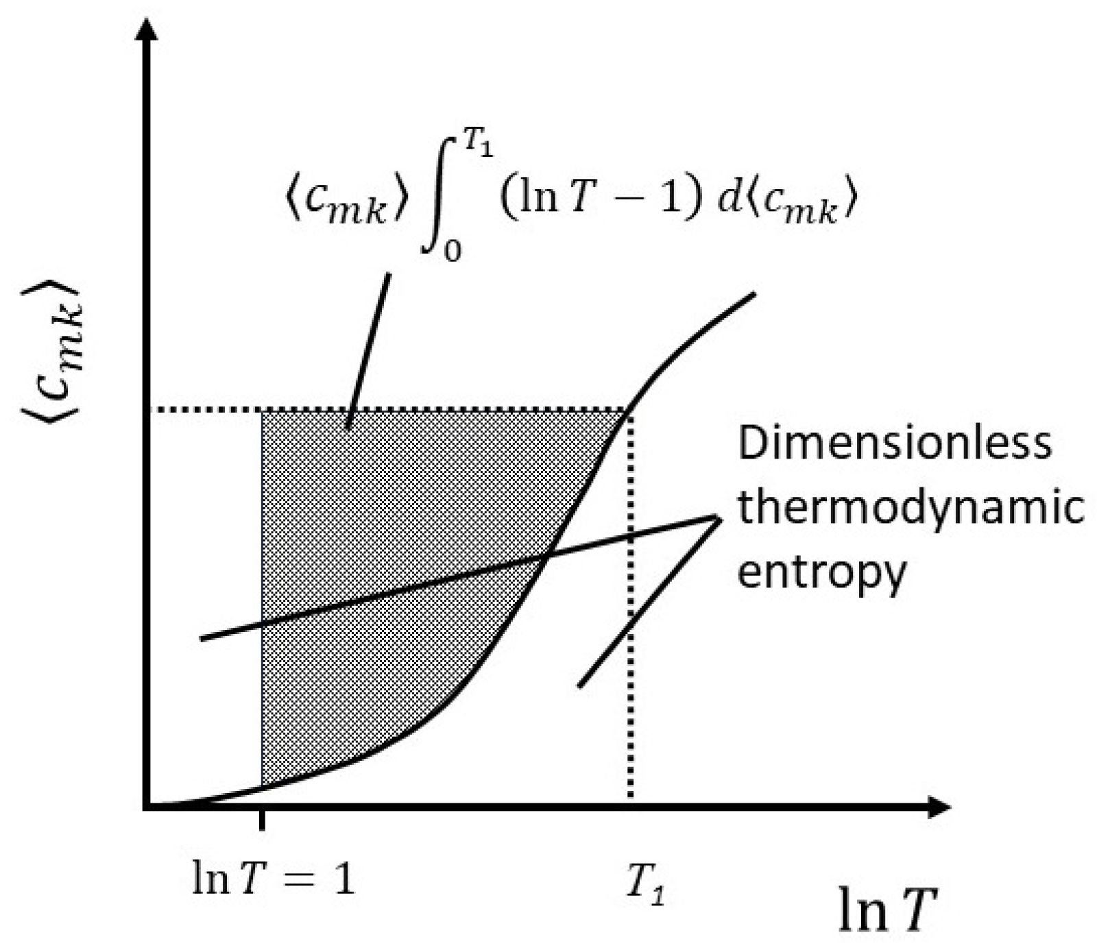
Figure 6.
The geometric representation of equation (40). Note that the molar heat capacity has not been made dimensionless, for direct comparison with Figure 3(b). The shape of the curve is intended to reflect the properties typical of simple liquids. It is well known that the heat capacity decreases with increasing temperature before rising again [14].
Disclaimer/Publisher’s Note: The statements, opinions and data contained in all publications are solely those of the individual author(s) and contributor(s) and not of MDPI and/or the editor(s). MDPI and/or the editor(s) disclaim responsibility for any injury to people or property resulting from any ideas, methods, instructions or products referred to in the content. |
© 2024 by the author. Licensee MDPI, Basel, Switzerland. This article is an open access article distributed under the terms and conditions of the Creative Commons Attribution (CC BY) license (https://creativecommons.org/licenses/by/4.0/).
Copyright: This open access article is published under a Creative Commons CC BY 4.0 license, which permit the free download, distribution, and reuse, provided that the author and preprint are cited in any reuse.


