
Submitted:
23 February 2024
Posted:
27 February 2024
Read the latest preprint version here
Abstract
Using assembly theory, we investigate assembly pathways of fixed-length binary strings formed by joining the individual bits present in the assembly pool and the strings that entered the pool as a result of previous joining operations. We show that the string assembly index is bounded from below and above. We derive the lower bound and conjecture the upper bound's form. We show that the length of an elegant binary program required to assemble a string featuring the smallest assembly index is equal to its assembly index, and conjecture that there is no binary program that has a length shorter than the length of the string featuring the largest assembly index that could assemble this string. We conjecture that a black hole surface is defined by a balanced distinct string that satisfies the upper bound of a distinct string assembly index. The results confirm that four Planck areas provide the minimum information capacity that provides a minimum thermodynamic (Bekenstein-Hawking) entropy. Knowing that the problem of determining the assembly index is at least NP-complete, we conjecture that the problem of determining the assembly index of a given binary string is NP-complete, while the problem of creating the string so that it would have a predetermined maximum assembly index is NP-hard. Therefore, once the new information is assembled by a dissipative structure or by a human, increasing the information entropy according to the second law of infodynamics, it is subject to the second law of thermodynamics, and nature seeks to optimize its assembly pathway.
Keywords:
assembly theory
; emergent dimensionality
; holographic principle
; black holes
; complexity measures
; P versus NP problem
; Gödel's incompleteness theorems
; halting problem
; elegant program
; quantum orthogonalization interval theorems
; second law of infodynamics
; mathematical physics
1. Introduction
Assembly Theory (AT) [1,2,3,4,5,6,7] provides a distinctive complexity measure, superior to established complexity measures used in information theory, such as Shannon entropy or Kolmogorov complexity [1,5]. AT does not alter the fundamental laws of physics [6]. Instead, it redefines objects on which these laws operate. In AT, objects are not considered as sets of point particles (as in most physics), but instead are defined by the histories of their formation (assembly pathways) as an intrinsic property, where, in general, there are multiple assembly pathways to create a given object.
AT explains and quantifies selection and evolution, capturing the amount of memory necessary to produce a given object [6]. This is because the more complex a given object is, the less likely an identical copy can be observed without the selection of some information-driven mechanism that generated that object. Formalizing assembly pathways as sequences of joining operations, AT begins with basic units (such as chemical bonds) and concludes with a final object. This conceptual shift captures evidence of selection in objects [1,2,6].
The Assembly Index, which represents the length of the shortest assembly pathway leading to an object, facilitates the quantification of the minimum memory required for its construction. In general, it increases with the object’s size, but decreases with symmetry, so large objects with repeating substructures may have lower complexity than smaller objects with greater heterogeneity [1]. The copy number specifies the number of copies of an object, essential for assessing its structural complexity.
AT has been experimentally confirmed in the case of molecules and probed directly experimentally with high accuracy with spectroscopy techniques, including mass spectroscopy, IR, and NMR spectroscopy [6]. It is a versatile concept with applications in various domains. Beyond its application in the field of biology and chemistry [7], its adaptability to different data structures, such as text, graphs, groups, music notations, image files, compression algorithms, etc., showcases its potential in diverse fields [2].
In this study, we investigate the assembly pathways of binary strings by joining individual bits present in the assembly pool [6] and strings that entered the pool as a result of previous joining operations.
| In particular, we investigate the assembly of black-body objects BBs (black holes (BHs), white dwarfs, and neutron stars) considered binary strings [8,9,10]. It is known [2,8,9,10,11,12,13,14,15,16,17,18,19] that information in the universe evolves toward increased structural complexity, decreasing information entropy. We use emphasis for object as this term, understood as a collection of matter, is a misnomer, as it neglects the (quantum) nonlocality [20]. Nonlocality is independent of the entanglement among particles [21], as well as the quantum contextuality [22], and increases as the number of particles [23] grows [24,25]. Furthermore, the ugly duckling theorem [26,27] asserts that every two objects we perceive are equally similar (or equally dissimilar). This study extends the findings of previous research [8,9,10,23] within the framework of AT [1,2,3,4,5,6,7] and emergent dimensionality [8,9,10,15,17,18,20,23]. However, our results generally apply to information theory. Therefore, we put the BB-related content in frames like this one. The reader not interested in BBs may skip the text in these frames and the additional results presented in Section 3. |
2. Results
We consider binary strings containing symbols , which are our basis AT objects [2], with zeros and ones, having a fixed length . We consider strings to be messages transmitted through a communication channel between a source and a receiver, similarly to the Claude Shannon approach used in the derivation of information entropy [28], and consider the process of their formation within the AT framework.
Definition 1.
A string assembly index is the smallest number of steps s required to assemble a binary string of length N by joining two basic symbols contained in the initial assembly pool and strings joined in previous steps that are added to the assembly pool. Therefore, the assembly index is a function of the string .
For example, the 8-bit string
- can be assembled in at most seven steps:
- 1.
- join 0 with 0 to form , adding to P,
- 2.
- join with 1 to form , adding to P,
- 3.
- ...
- 7.
- join with 1 to form ,
- six or five steps:
- join 0 with 0 to form , adding to P,
- join with 1 to form , adding to P,
- join with taken from P to form , adding to P,
- join with 0 to form , adding to P,
- join with 1 to form ,
- or at least four steps:
- join 0 with 1 to form , adding to P,
- join with 0 to form , adding to P,
- join with taken from P to form , adding to P,
- join with taken from P to form .
- Therefore, the string (1) has an assembly index that represents the length of the shortest assembly pathway leading to its assembly. cannot be assembled in a simpler way.
Definition 2.
A string is a balanced string if it has the same number of symbols, where or if N is odd.
Without loss of generality, we assume that if N is odd, (e.g., for , , and ). However, our results are equivalently applicable if we assume the opposite (i.e. a larger number of ones for an odd N).
The number of balanced strings among all strings is1
This is OEIS A001405 sequence, the maximal number of subsets of an N-set such that no one contains another, as asserted by Sperner’s theorem, and approximated using Stirling’s approximation for large N.
| BBs emit Hawking black-body radiation having a continuous spectrum that depends only on one factor, the BB temperature corresponding to the BB diameter , where and is the Planck length and temperature [8]. Triangulated BB surfaces contain a balanced number of Planck area triangles, each having binary potential , where c denotes speed of light in vacuum, as has been shown [8,10], based on the Bekenstein-Hawking entropy [29,30,31] . Here is the Boltzmann constant and is the information capacity of the BB surface, i.e., the Planck triangles corresponding to bits of information [8,9,10,30,32,33], and the fractional part triangle(s) having the area too small to carry a single bit of information [8,9]. Therefore, a balanced string represents a BB surface comprising active Planck triangles (APTs) with binary potential equal to [9]. |
Theorem 1.
A string having length is the shortest string having more than one string assembly index 1.
Proof.
The proof is trivial. For the assembly index , as all basis objects have a pathway assembly index of 0 [2] (they are not assembled). provides four available strings with . provides eight available strings with . Only provides 16 strings that include four stings with and twelve strings with including balanced strings, as shown in Table 1 and Table 2.
For example, to assemble the string we need to assemble the string and reuse it. Therefore, for and for , where denotes a set of different assembly indices. □
| Interestingly, Theorem 1 strengthens the meaning of as the minimum information capacity that provides a minimum thermodynamic (BH) entropy [29,30,31]. There is no disorder or uncertainty in an object that can be assembled in the same number of steps . |
In the following, we derive the tight lower bound of the set of different string assembly indices 1.
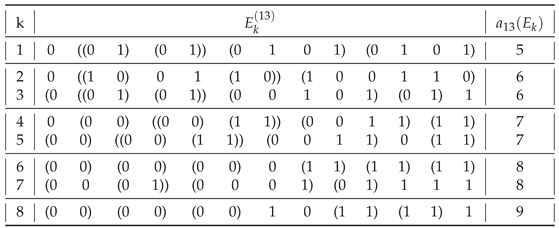
Table 1, Table A2, Table A3, Table A4, Table A5, Table A6, Table A7, Table A8 and Table A9 (Appendix C) show the distributions of the assembly indices among strings for taking into account the number of ones . The sums of each column form Pascal’s triangle read by rows (OEIS sequence A007318).
Theorem 2
(Tight lower bound on the string assembly index). The smallest string assembly index as a function of N is given by the OEIS sequence A014701.
Proof. 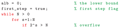
Strings for which , can be formed by joining two basic symbols, adding the pair to the pool and joining the longest strings taken from the pool until N is reached. Furthermore, if , then and only four strings provide such a minimal assembly index , , , and .
Therefore, we can use the following procedure
In other words, we recursively calculate the remainder of a division of N by the largest and increment the assembly index with every step s, noting that only at the first step it was equal to the largest s.
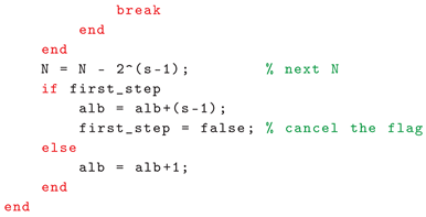
This procedure reflects the assembly of the string but gives the same as the procedure (OEIS A014701)
for the number of steps s to reach 1 starting from N. □
Theorem 3.
The length of an elegant binary program required to assemble a string featuring the smallest assembly index 2 is equal to its assembly index.
Proof.
An elegant program is the shortest program that produces a given output [34]. We assume that the assembly pool P is an ordered set and we define
Command 0: Take the last element from P, join it with itself, and output.
and
Command 1: Take the last two elements from P, join them with each other, and output.
as the only two commands applicable to the initial assembly pool containing only two basic symbols.
Then the program "" having a length of N bits will assemble the string having the assembly . Similarly, the program "" will assemble the string having . The remaining two strings and with can be assembled with the same two programs by reordering the initial assembly pool.
Furthermore, the remaining programs will assemble some of the shorter strings with the assembly index . For example, for the remaining six 3-bit programs will produce shorter strings with : six out of ten strings and four out of eighteen strings (and no string ), in total, ten strings as both "001" and "010" produce .
However, for , some of these programs are no longer elegant. For example, both programs "000" and "0111" assemble the string having the assembly index , but only the former is elegant. □
The binary assembly programs are listed in Table 3, Table 4 and Table 5 for one version of the assembly pool and for .
We note in passing that Theorem 3 would be violated if we defined the command "0" e.g. as "take the last element from the assembly pool, join it with itself, join with what you have already assembled (say at "the right"), and output". Then the 2-bit program "00" would produce with the assembly index . However, such a one-step command would violate the assumptions of assembly theory, as it would perform two assembly steps in one program step. An elegant program to output the gigabyte binary string of all zeros would take a few bits of code and would have a low Kolmogorov complexity [35]. However, such a string would be outputted, not assembled. Furthermore, the length of such a program that outputs the string would be shorter than the length of the program that outputs the string , while in AT, the lengths of these programs must be the same. Theorem 3 is about binputation2 of binary strings.
Theorem 3 is related to Gödel’s incompleteness theorems and the halting problem. N cases of the halting problem correspond only to , not to N bits of information [36]. Therefore, N-bit elegant programs assemble all four strings with (with two versions of the assembly pool). Furthermore, we can consider all strings assembled by our N-bit assembly program as corresponding to provable theorems. Any formal axiomatic system only enables proving only true theorems [37].There is a more fundamental path to incompleteness that involves complexity, rather than self-reference [37].
In the following, we conjecture the form of the upper bound of the set of different string assembly indices 1.
In general, of all strings having a given assembly index, shown in Table 1, Table A2, Table A3, Table A4, Table A5, Table A6, Table A7, Table A8 and Table A9, most are those having . The only exceptions are for () and for (), for () and for (), and for ().
Introducing the definition 2 of a balanced string allows us to reduce the search space of possible strings with maximal assembly indices to balanced strings only. With the exception of , of all strings having a maximum assembly index, most are balanced.
We can further restrict the search space to distinct strings.
Definition 3.
A string is a distinct string if a ring formed with this string by joining its beginning with its end is unique among the rings formed from the other distinct strings .
There are at least two and at most N forms of a distinct string that differ in the position of the starting symbol. For example for balanced strings, shown in Table 2, two augmented strings with correspond to each other if we change the starting symbol
Similarly, four augmented strings with correspond to each other
after a change in the position of the starting symbol. Thus, there are only two distinct strings for
The number of distinct strings among all strings is given by the OEIS sequence A000031. In general (for ), the number of distinct strings is much lower than the number of balanced strings.
| As asserted by the no-hair theorem [38], BH is characterized only by three parameters: mass, electric charge, and angular momentum. However, BHs are fundamentally uncharged and non-rotating, since the parameters of any conceivable BH, that is, charged (Reissner-Nordström), rotating (Kerr) and charged rotating (Kerr-Newman), can be arbitrarily altered, provided that the area of a BH surface does not decrease [39] using Penrose processes [40,41] to extract electrostatic and/or rotational energy of a BH [42]. Thus, a BH is defined by a single real number, and no Planck triangle is distinct on a BH surface. We can define neither a beginning nor an end of a balanced distinct string that represents a given BH. |
By neglecting the notion of the beginning and end of a string, we focus on its length and content. In Yoda’s language,
"complete, no matter where it begins. A message is".
The numbers of the balanced , distinct , and balanced distinct3 strings are shown in Table 6 and Figure 1.
We note that, in general, the starting symbol is relevant for the assembly index. Thus, different forms of a distinct string may have different assembly indices. For example, for balanced strings and , shown in Table A12 have . However, these strings are not distinct, since they correspond to each other and to the balanced strings , , , , and with . They all have the same triplet of adjoining ones.
Definition 4.
The assembly index of a distinct string is the smallest assembly index among all forms of this string.
Thus, if different forms of a distinct string have different assembly indices, we assign the smallest assembly index to this string. In other words, we assume that the smallest number of steps
where denotes a particular form of a distinct string , is the string assembly index of this distinct string.
| If an object that can be represented by a distinct string (a BB in particular) can be assembled in fewer steps, this procedure will be preferred by nature. |
The distribution of the assembly indices of the balanced distinct strings is shown in Table 7.
If a string for which is constructed from repeating patterns, then a string for which must be the most patternless. The string assembly index must be bounded from above and must be a monotonically nondecreasing function of N that can increase at most by one between N and .
Identifying the shortest pathway is known to be computationally challenging [3]. This problem has been proven to be at least as hard as NP-complete [43]. However, certain heuristic rules apply in our binary case. For example,
- for we cannot avoid two doublets (e.g. ) within a distinct string and thus ,
- for we cannot avoid two pairs of doublets (e.g. and ) within a distinct string and thus ,
- for we cannot avoid three pairs of doublets (e.g. , , and ) within a distinct string and thus ,
- for we cannot avoid two pairs of doublets and one doublet three times (e.g. , , and , and thus ,
- etc.
Conjecture 1.
The problem of determining the assembly index of a given binary stringis NP-complete [43], while the problem of creating the string so that it would have a predetermined maximum assembly index for this length of the string is NP-hard.
We found it much easier to determine an assembly index of a given binary string than to create a string so that it would have a maximum assembly index as a function of the length of the string. A proof of conjecture 1 would also be the proof of the following conjecture.
Conjecture 2.
Every computable problem and every computable solution can be encoded as a finite binary string. Here, determining whether the assembly index of a given string has its known maximal value corresponds to checking the solution to a problem for correctness, whereas creating such a string corresponds to solving the problem. Thus, AT would solve the P versus NP problem in theoretical computer science. There is ample pragmatic justification for adding as a new axiom [36].
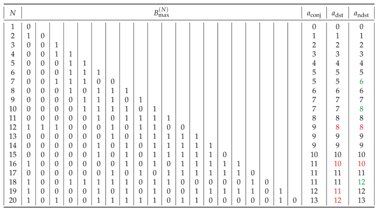
Table 8 shows the exemplary balanced strings having maximal assembly indices that we created (cf. also Appendix B). To determine the assembly index of the string
we look for the longest patterns that appear at least twice within the string, and we look for the largest number of these patterns. Here, we find that each of the two triplets and appear twice in and are based on the doublets and also appearing in . Thus, we start with the assembly pool made in four steps and join the elements of the pool in the following seven steps to arrive at . On the other hand, another form of this balanced distinct string
has .
Conjecture 3
(Tight upper bound on a string assembly index). With exceptions for small N the largest string assembly index of a binary string as a function of N is given by a sequence formed by strings for , where denotes increasing by one, and 0 denotes maintaining it at the same level, and .
However, at this moment, we cannot state if this conjecture applies to distinct or non-distinct strings. The assembly indices for are unique, whereas the assembly indices for were discussed above and are calculated in Appendix C for balanced and balanced distinct strings.
The conjectured sequence is shown in Figure 2 and Figure 3 starting with (we note in passing that is a dimension of the void, the empty set ∅, or (-1)-simplex). Subsequent terms are given by , which is periodic for and flattens at , and , , .
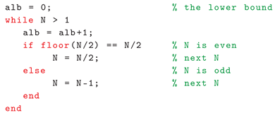
This sequence can be generated using the following procedure
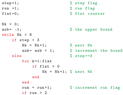
We note the similarity of this bound to the Aufbau rule4, the Janet sequence (OEIS A167268) and the monotonically non-decreasing Shannon entropy of chemical elements, including observable ones [23]. Perhaps the exceptions in the sequence 3 vanish as N increases.
The bounds 2 and 3 are shown in Table 6 and illustrated in Figure 2 and Figure 3. No binary string cannot be assembled in a smaller number of steps than given by the bound 2 On the other hand, some strings cannot be assembled in a smaller number of steps than given by an upper bound (which for large N, as we suppose, has the form presented in Conjecture 3).
Conjecture 4.
There is no binary program that has a length shorter than the length of the string featuring the largest assembly index that could assemble this string.
Partial Proof.
In assembling the string featuring the assembly index (the largest complexity), we cannot rely solely on the last or two last strings in the assembly pool. Thus, we need to index the strings in the pool. However, we cannot predict in advance how many strings there will be in the assembly pool. Thus, we do not know how many bits will be needed to encode the indices. □
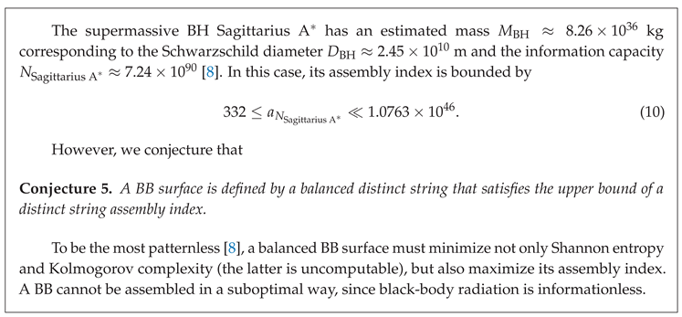
The Hamlet tragedy contains approximately 130,000 letters. Assigning five bits per letter (32 possibilities), the Hamlet tragedy can be encoded in a string having bits (81.25 kB) yielding the total number of possible strings (including ), and their assembly indices are bounded by
The lower bound (8) can be calculated directly using the procedures of Theorem 2. The upper bound (8) can be estimated by finding the smallest k that satisfies and using the relation of Conjecture 3.
We assume that the assembly index of the string encoding the actual Hamlet tragedy is close to the upper bound. Even if the probability of random typing of the Hamlet tragedy is unfathomably small, when constrained to the bounds of the physical universe [5], as asserted by the infinite monkey theorem, this tragedy was once created by William Shakespeare.
SARS-CoV-2 genome sequence contains 29903 bases . Assigning two bits per base it can be encoded in a string of bits having the assembly index bounded by
3. Additional results
The [perceivable] universe is not big enough to contain the future; it is deterministic going back in time and non-deterministic going forward in time [44]. But we know [2,8,9,10,11,12,13,14,15,16,17,18,19] that it has evolved to the present since the Big Bang.
For K subunits of an object O the assembly index of AT is bounded [1] from below by
and from above by
where in the latter case, the subunits must be distinct so that they could not be reused from the pool, decreasing the index. The lower bound (11) represents the fact that the simplest way to increase the size of an object in a pathway is to take the largest object so far and join it to itself [1]. However, for and .
Perceivable information about any object can be encoded by a binary string [26,27]. This does not imply that a binary string defines an object. Information that defines a chemical compound, a virus, a computer program, etc. can be encoded by a binary string. However, a dissipative structure [12] such as a living biological cell (or its conglomerate such as a human, for example) cannot be represented by a binary string (even if its genome can). This information can only be perceived (so this is not an object defining information). Each of us is given to ourselves as a mystery [45]. Therefore, since one bit is the smallest amount and the quantum of information, the lower bound 2 and the upper bound of the string assembly index define the allowed region of the assembly indices for binary strings.
The bounds 2, 3, (11), and (12) on the assembly index are shown also in Figure 4 (adopted from [1] and modified). According to the authors of [1], the "green portion of the figure is illustrative of the location in the complexity space where life might reasonably be found. Regions below can be thought of as being potentially naturally occurring, and regions above being so complex that even living systems might have been unlikely to create them. This is because they represent structures with limited internal structure and symmetries, which would require vast amounts of effort to faithfully reproduce." [1].
We disagree with this statement. It is obvious that a binary string itself is neither dissipative nor creative. It is its assembly process that can be dissipative or creative. Evolution is about assembling new information and optimizing it until it reaches its assembly index.
That is why, we found determining the assembly index of a given binary string is easier than creating a string with a maximum assembly index for this length of the string (Conjecture 1). Once the new information is assembled (by a dissipative structure operating far from thermodynamic equilibrium, or created by humans) increasing the information entropy according to the 2nd law of infodynamics [16], it enters the realm of the 2nd law of thermodynamics, and nature seeks how to optimize its assembly pathway decreasing information entropy. And only humans are gifted with creativity. Any creation is required to be shaped by the unique personality of the creator to such an extent that it is statistically one-time in nature [46]; it is an imprint of the author’s personality.
The total entropy of the universe S is constant and is the sum of the information entropy and the physical entropy . Therefore, over time [19]
The time corresponds to an increasing information capacity. Bit by bit:
At first, the newly assembled information corresponds to the discovery by groping [11]. However, its assembly pathway does not attain its most economical or efficient form all at once. For a certain period of time, its evolution gropes about within itself. The try-out follows the try-out, not being finally adopted. Then finally perfection comes within sight, and from that moment the rhythm of change slows down [11]. The new information, having reached the limit of its potentialities, enters the phase of conquest. Stronger now than its less perfected neighbours, the new information multiplies and consolidates. When the assembly index is reached, new information attains its equilibrium (not necessarily a BH equilibrium) and its evolution terminates. It becomes stable.
There is a certain minimum amount of information required to establish a creation, as shown in Figure 4. Sixteen possibilities provided by the minimum of thermodynamic entropy [29,30,31] bifurcate the assembly pathways (cf. Theorem 1) but none of these possibilities can be considered a creation. However, the boundary between the green region of dissipative structures [12] and the red region of human creativity remains to be discovered.
"Thanks to its characteristic additive power, living matter (unlike the matter of the physicists) finds itself ’ballasted’ with complications and instability. It falls, or rather rises, towards forms that are more and more improbable. Without orthogenesis life would only have spread; with it there is an ascent of life that is invincible." [11]
BB having the energy given by mass-energy equivalence
where , denote the BB mass, and , denote the Planck energy and mass, is the fine-structure constant and is the fine-structure constant related to by , and k is the BB size-to-mass ratio (STM) [10] ( if BB is BH).
It was shown [9] based on the Mandelstam-Tamm [47], Margolus–Levitin [48], and Levitin-Toffoli [49] theorems on the quantum orthogonalization interval that BBs generate (or rather assemble) a pattern forming nonequilibrium shell (VS) through the solid-angle correspondence, as shown in Figure 5. The BB entropic work
is the work done by all APTs of a BB. It is the product of the BB entropy [29,30,31] and the general, complex BB temperature
which in modulus and for a BH () reduces [10] to Hawking temperature
where is the reduced Planck constant, G is the gravitational constant, and is the Planck temperature. In particular [10]
where
is the energy equilibrium STM.
A VS has the information capacity bounded by
where l is a VS defining factor. The number of APTs is bounded by
as shown in Figure 6, and thus its binary potential [8,9] is bounded by
and the theoretical probability for a triangle on a VS to be an active Planck triangle is also bounded [9] by
On the other hand, the entropy variation [8,50] so that for the lower bound (24) is negative and the upper bound (23) is positive ( in this range). The Planck triangle of VS is located somewhere on the VS surface defined by a solid angle
that corresponds to the BB Planck triangle.
The BB information capacity is dictated by its diameter and the BB energy (14) as a function of its diameter is the same for all BBs (it is independent on k). However, the BB mass and density
are not.
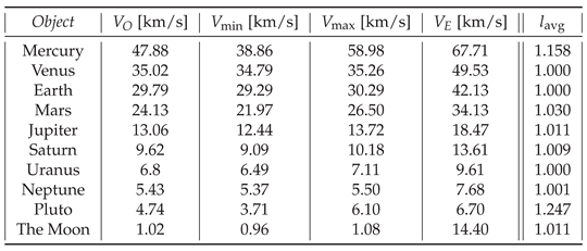
Based on the orbiting condition , where is the orbital, and the escape speed of an orbiting object, is the average distance from the center of the central object to the center of the orbiting object, and is the mass of the central object, the bounds
containing the velocity term , were also derived [9]. Plugging from the bounds (21) into the bounds (27) we arrive at
which is satisfied by real and imaginary (but not complex) velocities (for example, for by , , , and ). Taking the square root of the bounds (28), using , [9], and squaring again, we arrive at
The bounds (28) and (29), shown in Figure 7, meet at , where de Broglie and Compton wavelengths of mass M are the same
where p is the relativistic momentum. The same is the ratio of orbital to escape speed: .
Furthermore, the bounds (28) and (29) do not overlap only for . Therefore, defines the dissipativity or the assembly range. Furthermore, the intersection of the bounds (28) and (29) is the common region for both velocities. If is within this region, then is as well. We note that the average orbital velocity of each orbiting object only slightly exceeds its orbital speed . This implies that the average VS defining factor in (21) for a VS orbiting object (cf. Appendix A).
BBs define a perfect thermodynamic equilibrium, and the bounds (21) and (22) show that nature uses optimally assembled information (cf. Conjecture 5) to assemble new information. Figure 8 shows the bounds on the string assembly indices, and Figure 9 shows the BB temperature (17), energy (14), and entropic work (15) for . is a rational number for natural .
Let us examine this process starting from the Big Bang during the Planck epoch and shortly thereafter, and for continuous (i.e., including fractional Planck triangle(s)).
There is nothing to talk about. It is a mystery.
The Big Bang has occurred, forming the 1st BB. At the BB temperature (17) and subsequently at the BH temperature (17) become equal to the Planck temperature, but any BB in this range is still too small to carry a single bit of information and cannot be triangulated. However, independent BBs merge [9,10] summing their entropies and increasing the information capacity.
The first bit (a degree of freedom [9]) becomes available, and the BH energy reaches the limit of the equipartition theorem for one bit (). APTs on BBs begin to fluctuate. However, the bounds (22) make them unable to generate any APTs on a VS ().
The BH temperature (17) exceeds its energy (14) () [9]. At the BH energy (14) is equal to the Landauer limit [51]. Shortly thereafter, at , the BH density reaches the level of the Planck density For a BB [10] Still . Merging BBs expand fractional Planck triangle(s) to form the 2nd bit.
The first nonvanishing becomes available on a VS generated by a BB. The BH temperature (17) is equal to its energy (14) ().
At the BH entropic work (15) is equal to the Landauer limit (). At the density of the least dense BB () drops below the modulus of its temperature. .
With BBs can finally be triangulated. Yet, containing only one APT (), they are not ergodic [9].
At the BH surface gravity drops below the Planck acceleration and the tangential acceleration [8,9] becomes real ().
The BB assembly index bifurcates, minimal thermodynamic entropy [30] is reached, and the relation (22) provides the second bit on a VS (). At this moment BB can be assembled in a different number of steps and nature seeks to minimize this number following the dynamics induced by the relation (13). The BH temperature (17) is equal to its entropic work (15) ().
A BB reaches the upper bound on distinct assembly index.
The imaginary Planck time appears at the BH surface [8] heralding the end of the Planck epoch. After crossing this threshold, the VSs begin to operate with on , and the first dissipative structures can be assembled.
Nature enters a directed exploration phase () and selectivity emerges, limiting the discovery of new objects [6].
A BB reaches the upper bound on nondistinct assembly index.
- …
At a first precise diameter relation can be established between the vertices of the BB surface. Furthermore, for , the solid angle (25) equals one steradian.
-
⋯
The onset of human creativity.
4. Conclusions
The results reported here can be applied in the fields of cryptography, data compression methods, stream ciphers, approximation algorithms [52], reinforcement learning algorithms [53], information-theoretically secure algorithms, etc. Another possible application of the results of this study could be molecular physics and crystallography.
| Overall, the results reported here support the assembly theory [1,2,3,4,5,6,7], the Bekenstein’s minimum of thermodynamic entropy [29,30,31], the holographic principle [32], entropic gravity [33], emergent dimensionality [8,9,10,15,17,18,20,23], the second law of infodynamics [16,19], and invite further research. |
Author Contributions
WB: Conjecture concerning the diversification of strings in Theorem 3; partitioning conjecture for resulting in the flattening of the string assembly index upper bound curve; observation that the string assembly index upper bound curve should BE monotonically non-decreasing; linear interpolation of VS defining factors; prior-art search; numerous clarity corrections and improvements; SŁ: The remaining part of the study.
Data Availability Statement
The public repository for the code written in MATLAB computational environment is given under the link https://github.com/szluk/Evolution_of_Information (accessed on November 23, 2023).
Acknowledgments
The authors thank Piotr Masierak for his creative remarks on the definition of a distinct string 3, research on the general strategy for determining the string assembly indices, and creating the string (Peter’s rock), Andrzej Tomski for a clarity correction, and Mariola Bala for noting that "this is logical". SŁ thanks his wife Magdalena Bartocha for her unwavering support and motivation and his partner and friend, Renata Sobajda, for her prayers.
Abbreviations
The following abbreviations are used in this manuscript:
| AT | assembly theory; |
| BH | black hole; |
| BB | black-body object (BH, white dwarf, neutron star); |
| VS | nonequilibrium shell; |
| APT | active Planck triangle; |
| N | length of a binary string; |
| number of 0’s in the binary string; | |
| number of 1’s in the binary string (number of APTs); | |
| assembly index of a string of length N; | |
| binary string of length N; | |
| balanced string of length N; | |
| distinct string of length N; | |
| balanced distinct string of length N; | |
| number of binary strings of length N (); | |
| number of balanced strings of length N (OEIS A001405); | |
| number of distinct strings (OEIS A000031); | |
| number of balanced distinct strings; | |
| length of a balanced binary string (BB surface); | |
| s | assembly step. |
Appendix A. Orbital velocities and the VS defining factor l
Table A1 shows the orbital speed and escape speed of some celestial objects, their minimal and maximal velocities5. The former ones lie below the orbital speed limits. The average VS defining factor , where were determined by linear interpolation.

Table A1.
Exemplary orbital speeds and velocities, and the average VS defining factor .
 |
Appendix B. Exemplary strings with maximal assembly indices
For the exemplary balanced distinct strings , shown in Table 8:
- all forms of have ,
- all forms of have ,
- all forms of have ,
- the form has but the form has ,
- all forms of have ,
- all forms of have ,
- the form has but the form has ,
- all forms of have ,
- all forms of have ,
- all forms of have ,
- all forms of have ,
- all forms of have ,
- all forms of have ,
- all forms of have ,
- all forms of have ,
- some forms of have ,
- some forms of have .
Appendix C. Binary strings and their assembly indices
Table A2, Table A3, Table A4, Table A5, Table A6, Table A7, Table A8 and Table A9 show distributions of the assembly indices for . Table A10, Table A11, Table A12, Table A13 and Table A14 show balanced strings and their assembly indices for . Table A15, Table A16, Table A17, Table A18, Table A19 and Table A20 show the balanced distinct strings and their assembly indices for . Table A21, Table A22 and Table A23 show selected balanced distinct strings and their assembly indices for .
Table A2.
Distribution of the assembly indices for .
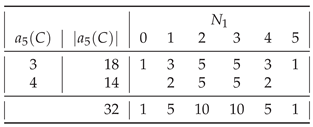 |
Table A3.
Distribution of the assembly indices for .
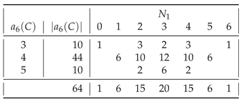 |
Table A4.
Distribution of the assembly indices for .
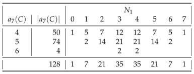 |
Table A5.
Distribution of the assembly indices for .
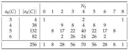 |
Table A6.
Distribution of the assembly indices for .
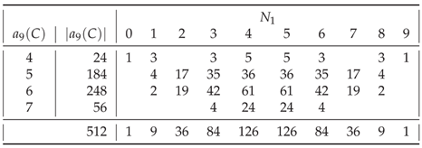 |
Table A7.
Distribution of the assembly indices for .
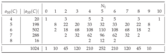 |
Table A8.
Distribution of the assembly indices for .
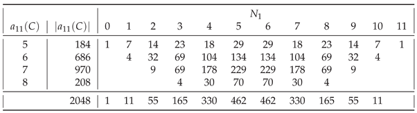 |
Table A9.
Distribution of the assembly indices for .
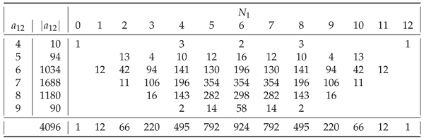 |
Table A10.
balanced strings.
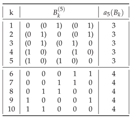 |
Table A11.
balanced strings.
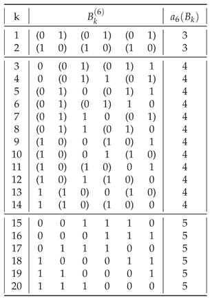 |
Table A12.
balanced strings.
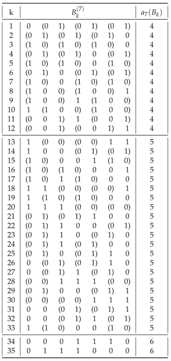 |
Table A13.
balanced strings (1st part).
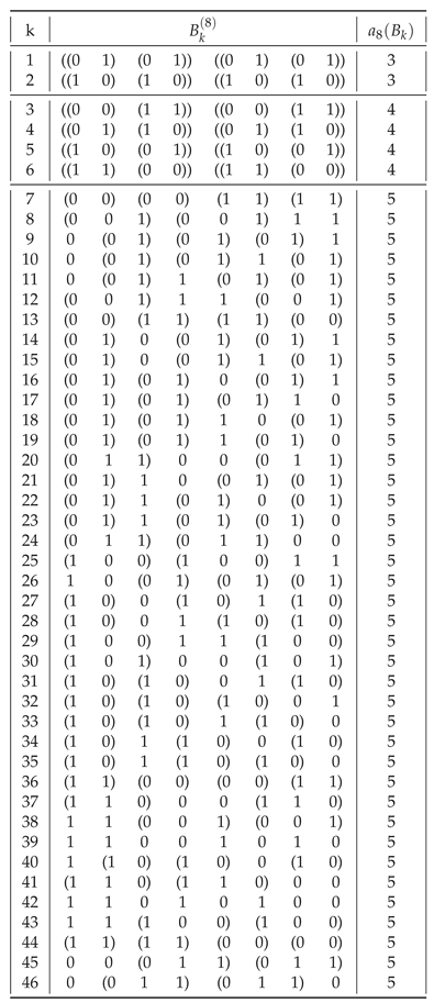 |
Table A14.
balanced strings (2nd part).
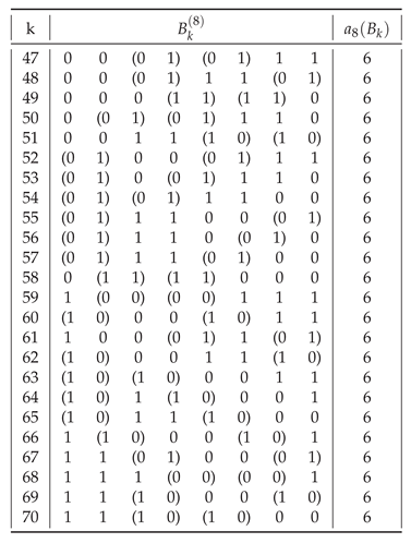 |
Table A15.
balanced distinct strings.
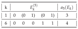 |
Table A16.
balanced distinct strings.
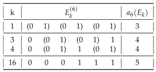 |
Table A17.
balanced distinct strings.
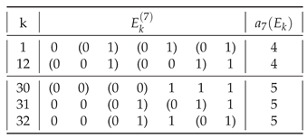 |
Table A18.
balanced distinct strings.
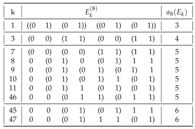 |
Table A19.
Selected balanced distinct strings .
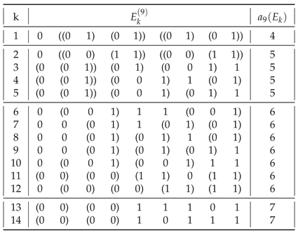 |
Table A20.
balanced distinct strings.
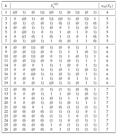 |
Table A21.
Selected balanced distinct strings .
 |
Table A22.
Selected balanced distinct strings .
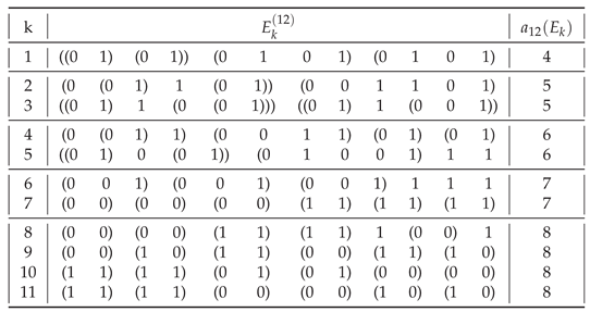 |
Table A23.
Selected balanced distinct strings .
 |
References
- Marshall, S.M.; Murray, A.R.G.; Cronin, L. A probabilistic framework for identifying biosignatures using Pathway Complexity. Philosophical Transactions of the Royal Society A: Mathematical, Physical and Engineering Sciences 2017, 375, 20160342. [Google Scholar] [CrossRef] [PubMed]
- Murray, A.; Marshall, S.; Cronin, L. Defining Pathway Assembly and Exploring its Applications, 2018. arXiv:1804.06972 [cs, math].
- Marshall, S.M.; Mathis, C.; Carrick, E.; Keenan, G.; Cooper, G.J.T.; Graham, H.; Craven, M.; Gromski, P.S.; Moore, D.G.; Walker, S.I.; Cronin, L. Identifying molecules as biosignatures with assembly theory and mass spectrometry. Nature Communications 2021, 12, 3033. [Google Scholar] [CrossRef] [PubMed]
- Liu, Y.; Mathis, C.; Bajczyk, M.D.; Marshall, S.M.; Wilbraham, L.; Cronin, L. Exploring and mapping chemical space with molecular assembly trees. Science Advances 2021, 7, eabj2465. [Google Scholar] [CrossRef] [PubMed]
- Marshall, S.M.; Moore, D.G.; Murray, A.R.G.; Walker, S.I.; Cronin, L. Formalising the Pathways to Life Using Assembly Spaces. Entropy 2022, 24, 884. [Google Scholar] [CrossRef] [PubMed]
- Sharma, A.; Czégel, D.; Lachmann, M.; Kempes, C.P.; Walker, S.I.; Cronin, L. Assembly theory explains and quantifies selection and evolution. Nature 2023, 622, 321–328. [Google Scholar] [CrossRef] [PubMed]
- Jirasek, M.; Sharma, A.; Bame, J.R.; Mehr, S.H.M.; Bell, N.; Marshall, S.M.; Mathis, C.; Macleod, A.; Cooper, G.J.T.; Swart, M.; Mollfulleda, R.; Cronin, L. Determining Molecular Complexity using Assembly Theory and Spectroscopy, 2023. arXiv:2302.13753 [physics, q-bio].
- Łukaszyk, S. , Black Hole Horizons as Patternless Binary Messages and Markers of Dimensionality. In Future Relativity, Gravitation, Cosmology; Nova Science Publishers, 2023; chapter 15, pp. 317–374. [CrossRef]
- Łukaszyk, S. Life as the Explanation of the Measurement Problem. Journal of Physics: Conference Series 2024, 2701. [Google Scholar] [CrossRef]
- Łukaszyk, S. The Imaginary Universe. preprint, PHYSICAL SCIENCES, 2023.
- de Chardin, P.T. The Phenomenon of Man; Harper, New York, 1959.
- Prigogine, I.; Stengers, I. Order out of Chaos: Man’s New Dialogue with Nature; Bantam Books, 1984.
- Melamede, R. Dissipative Structures and the Origins of Life. Unifying Themes in Complex Systems IV; Minai, A.A.; Bar-Yam, Y., Eds.; Springer Berlin Heidelberg: Berlin, Heidelberg, 2008; pp. 80–87.
- Vedral, V. Decoding Reality: The Universe as Quantum Information; Oxford University Press, 2010. [CrossRef]
- Łukaszyk, S. Four Cubes, 2020. [CrossRef]
- Vopson, M.M.; Lepadatu, S. Second law of information dynamics. AIP Advances 2022, 12, 075310. [Google Scholar] [CrossRef]
- Łukaszyk, S. Novel Recurrence Relations for Volumes and Surfaces of n-Balls, Regular n-Simplices, and n-Orthoplices in Real Dimensions. Mathematics 2022, 10. [Google Scholar] [CrossRef]
- Łukaszyk, S.; Tomski, A. Omnidimensional Convex Polytopes. Symmetry 2023, 15. [Google Scholar] [CrossRef]
- Vopson, M.M. The second law of infodynamics and its implications for the simulated universe hypothesis. AIP Advances 2023, 13, 105308. [Google Scholar] [CrossRef]
- Łukaszyk, S. A No-go Theorem for Superposed Actions (Making Schrödinger’s Cat Quantum Nonlocal). In New Frontiers in Physical Science Research Vol. 3; Purenovic, D.J., Ed.; Book Publisher International (a part of SCIENCEDOMAIN International), 2022; pp. 137–151. [CrossRef]
- Qian, K.; Wang, K.; Chen, L.; Hou, Z.; Krenn, M.; Zhu, S.; Ma, X.s. Multiphoton non-local quantum interference controlled by an undetected photon. Nature Communications 2023, 14, 1480. [Google Scholar] [CrossRef] [PubMed]
- Xue, P.; Xiao, L.; Ruffolo, G.; Mazzari, A.; Temistocles, T.; Cunha, M.T.; Rabelo, R. Synchronous Observation of Bell Nonlocality and State-Dependent Contextuality. Physical Review Letters 2023, 130, 040201. [Google Scholar] [CrossRef]
- Łukaszyk, S. Shannon Entropy of Chemical Elements. European Journal of Applied Sciences 2024, 11, 443–458. [Google Scholar] [CrossRef]
- Tran, D.M.; Nguyen, V.D.; Ho, L.B.; Nguyen, H.Q. Increased success probability in Hardy’s nonlocality: Theory and demonstration. Phys. Rev. A 2023, 107, 042210. [Google Scholar] [CrossRef]
- Colciaghi, P.; Li, Y.; Treutlein, P.; Zibold, T. Einstein-Podolsky-Rosen Experiment with Two Bose-Einstein Condensates. Phys. Rev. X 2023, 13, 021031. [Google Scholar] [CrossRef]
- Watanabe, S. Knowing and Guessing: A Quantitative Study of Inference and Information; Wiley, 19691969.
- Watanabe, S. Epistemological Relativity. Annals of the Japan Association for Philosophy of Science 1986, 7, 1–14. [Google Scholar] [CrossRef]
- Shannon, C.E. A Mathematical Theory of Communication. Bell System Technical Journal 1948, 27, 379–423. [Google Scholar] [CrossRef]
- Bekenstein, J.D. Black holes and the second law. Lettere Al Nuovo Cimento Series 2 1972, 4, 737–740. [Google Scholar] [CrossRef]
- Bekenstein, J.D. Black Holes and Entropy. Phys. Rev. D 1973, 7, 2333–2346. [Google Scholar] [CrossRef]
- Hawking, S.W. Particle creation by black holes. Communications In Mathematical Physics 1975, 43, 199–220. [Google Scholar] [CrossRef]
- Hooft, G.t. Dimensional Reduction in Quantum Gravity, 1993. [CrossRef]
- Verlinde, E. On the origin of gravity and the laws of Newton. Journal of High Energy Physics 2011, 2011, 29. [Google Scholar] [CrossRef]
- Chaitin, G.J. The unknowable; Springer series in discrete mathematics and theoretical computer science, Springer: Singapore ; New York, 1999.
- Kolmogorov, A. On tables of random numbers. Theoretical Computer Science 1998, 207, 387–395. [Google Scholar] [CrossRef]
- Chaitin, G. From Philosophy to Program Size: Key Ideas and Methods : Lecture Notes on Algorithmic Information Theory from the 8th Estonian Winter School in Computer Science, EWSCS’03 : [2-7 March]; Institute of Cybernetics at Tallinn Technical University, 2003.
- Chaitin, G. Complexity and metamathematics, 2023.
- Misner, C.W.; Thorne, K.S.; Wheeler, J.A. Gravitation; W. H. Freeman: San Francisco, 1973.
- Gould, A. Classical derivation of black-hole entropy. Physical Review D 1987, 35, 449–454. [Google Scholar] [CrossRef] [PubMed]
- Penrose, R.; Floyd, R.M. Extraction of Rotational Energy from a Black Hole. Nature Physical Science 1971, 229, 177–179. [Google Scholar] [CrossRef]
- Christodoulou, D.; Ruffini, R. Reversible Transformations of a Charged Black Hole. Physical Review D 1971, 4, 3552–3555. [Google Scholar] [CrossRef]
- Stuchlík, Z.; Kološ, M.; Tursunov, A. Penrose Process: Its Variants and Astrophysical Applications. Universe 2021, 7, 416. [Google Scholar] [CrossRef]
- Liu, Y.; Mathis, C.; Marshall, S.; Bajczyk, M.D.; Wilbraham, L.; Cronin, L. Exploring and Mapping Chemical Space with Molecular Assembly Trees. preprint, Chemistry, 2021. [CrossRef]
- Cronin, Leroy. Lee Cronin: Controversial Nature Paper on Evolution of Life and Universe | Lex Fridman Podcast #404, 2023. Accessed: 2023-12-18.
- Zatorski, W. W życiu chodzi o życie, wydanie i ed.; Tyniec Wydawnictwo Benedyktynów: Kraków, 2020. OCLC: 1243002797.
- Barta, J.; Markiewicz, R., Eds. Prawo autorskie: przepisy, orzecznictwo, umowy miedzynarodowe, wyd. 4., rozsz. i zaktualizowane ed.; Dom Wydawniczy ABC: Warszawa, 2002.
- Mandelstam, L.; Tamm, I. The Uncertainty Relation Between Energy and Time in Non-relativistic Quantum Mechanics. J. Phys. (USSR) 1945, 9, 249–254. [Google Scholar]
- Margolus, N.; Levitin, L.B. The maximum speed of dynamical evolution. Physica D: Nonlinear Phenomena 1998, 120, 188–195. [Google Scholar] [CrossRef]
- Levitin, L.B.; Toffoli, T. Fundamental Limit on the Rate of Quantum Dynamics: The Unified Bound Is Tight. Physical Review Letters 2009, 103, 160502. [Google Scholar] [CrossRef]
- Hossenfelder, S. Comments on and Comments on Comments on Verlinde’s paper "On the Origin of Gravity and the Laws of Newton", 2010. arXiv:1003.1015 [gr-qc].
- Landauer, R. Irreversibility and Heat Generation in the Computing Process. IBM Journal of Research and Development 1961, 5, 183–191. [Google Scholar] [CrossRef]
- Łukaszyk, S. A new concept of probability metric and its applications in approximation of scattered data sets. Computational Mechanics 2004, 33, 299–304. [Google Scholar] [CrossRef]
- Castro, P.S.; Kastner, T.; Panangaden, P.; Rowland, M. MICo: Improved representations via sampling-based state similarity for Markov decision processes. Advances in Neural Information Processing Systems 2021, 34, 30113–30126. [Google Scholar] [CrossRef]
| 1 | "" is the floor function that yields the greatest integer less than or equal to x and "" is the ceiling function that yields the least integer greater than or equal to x. |
| 2 | As an analog to chemputation, where assembly theory is applied to chemistry. |
| 3 |
is close to OEIS A000014 up to the eleventh term. |
| 4 | Only about twenty chemical elements (with only two nondoubleton sets of consecutive ones) violate the Aufbau rule. |
| 5 | Based on https://sci.esa.int/web/solar-system. |
Figure 1.
Numbers of all strings (red), balanced strings (green), distinct strings (cyan), and balanced distinct strings (blue) as a function of the string length N.
Figure 1.
Numbers of all strings (red), balanced strings (green), distinct strings (cyan), and balanced distinct strings (blue) as a function of the string length N.
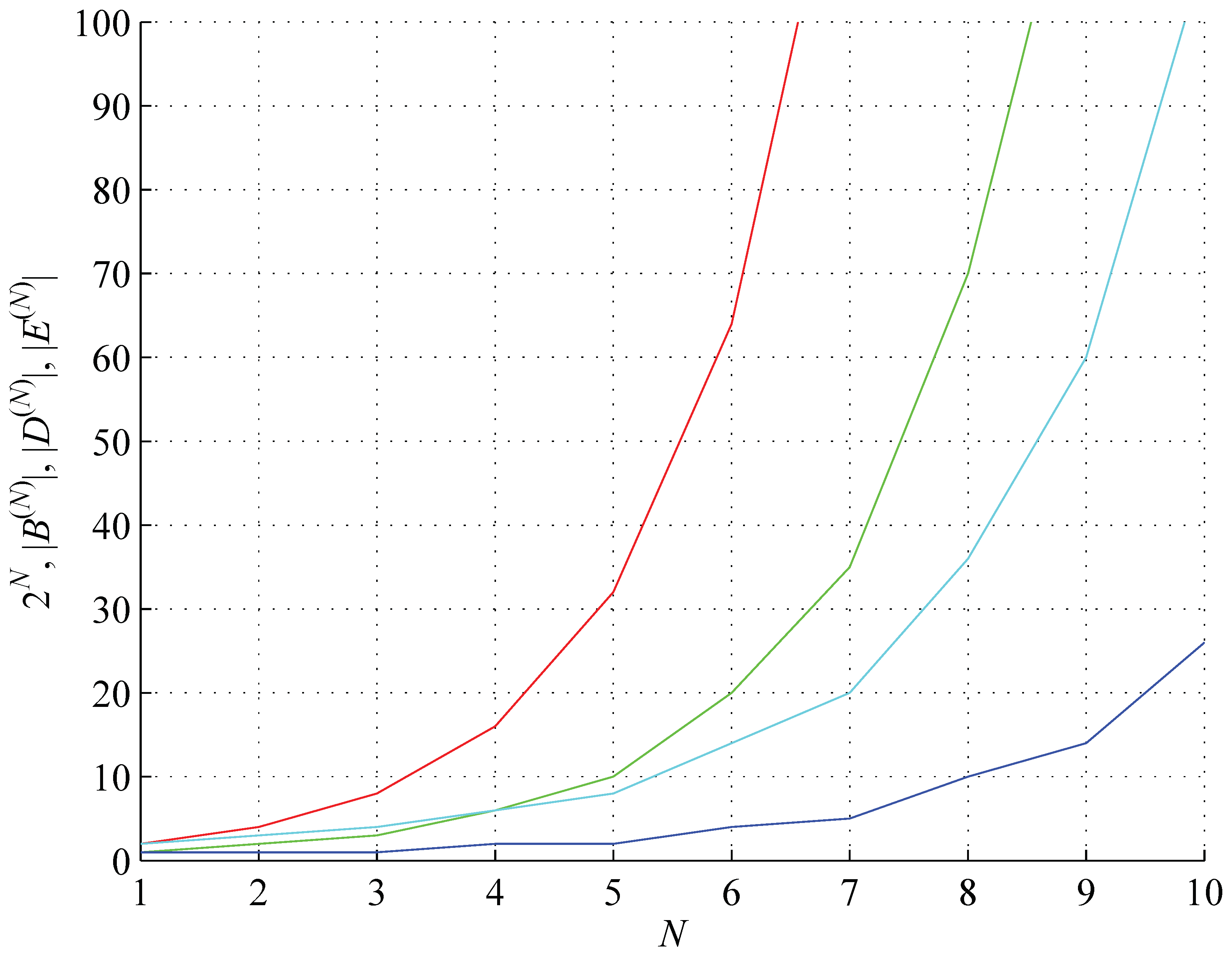
Figure 2.
Tight lower bound on the binary string assembly index 2 (red) and (red, dash-dot), conjectured upper bound on the binary string assembly index 3 (green), factual values of the string assembly index (blue) and the distinct string assembly index (cyan) and (green, dash-dot), for the string length .
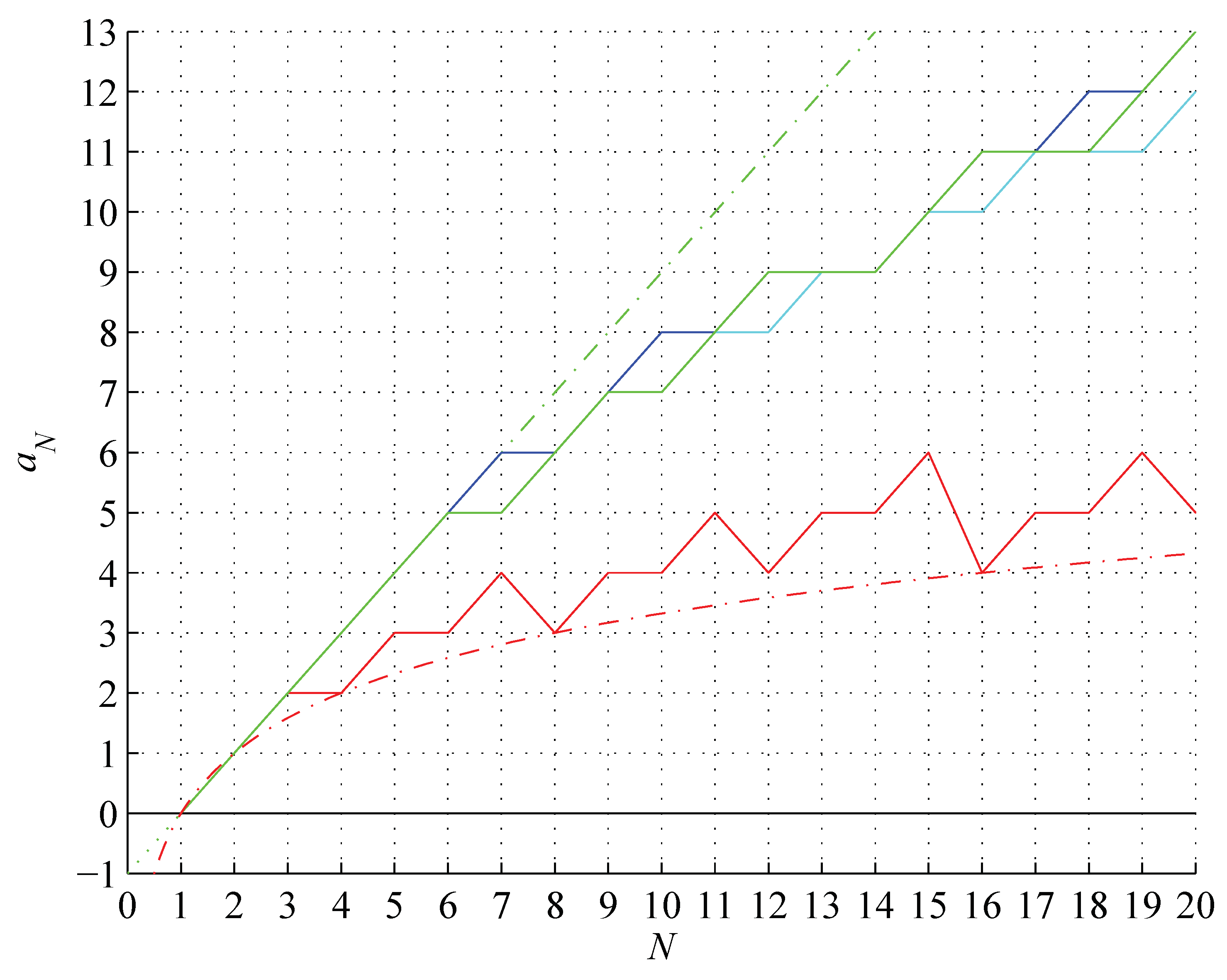
Figure 3.
Tight lower bound on the binary string assembly index (red) and (red, dash-dot), conjectured upper bound on the string assembly index (green) and (green, dash-dot), for the binary string length .
Figure 3.
Tight lower bound on the binary string assembly index (red) and (red, dash-dot), conjectured upper bound on the string assembly index (green) and (green, dash-dot), for the binary string length .

Figure 4.
An illustrative graph of complexity against information capacity: orange regions are impossible, as they are above or below the assembly bounds; yellow region contains structures optimally assembled (in equilibrium); green region contains dissipative structures; and red region is the region of human creativity (figure not to scale).
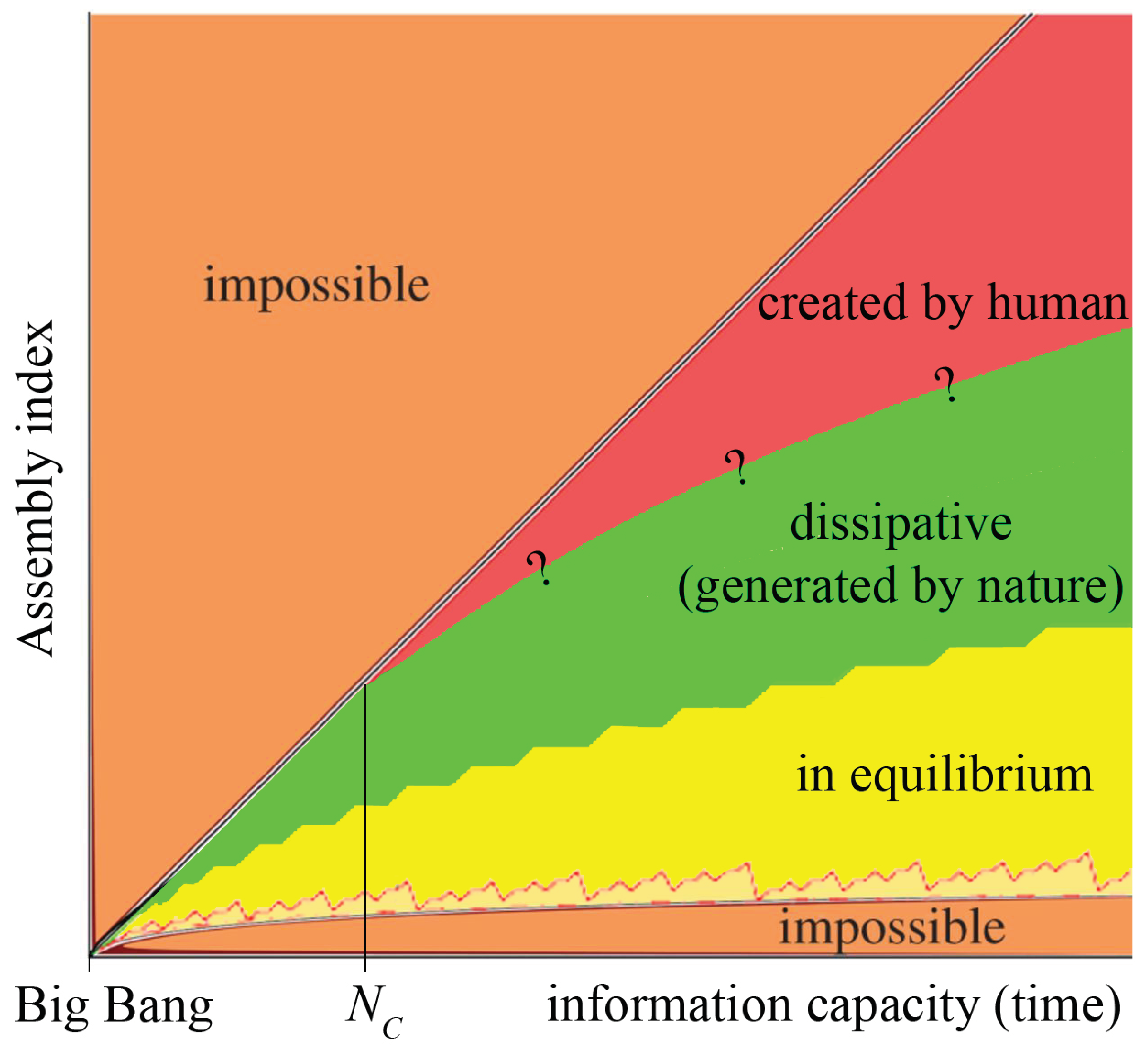
Figure 5.
A black body object as a generator of an entropy variation shell (VS) through the solid angle correspondence.
Figure 5.
A black body object as a generator of an entropy variation shell (VS) through the solid angle correspondence.
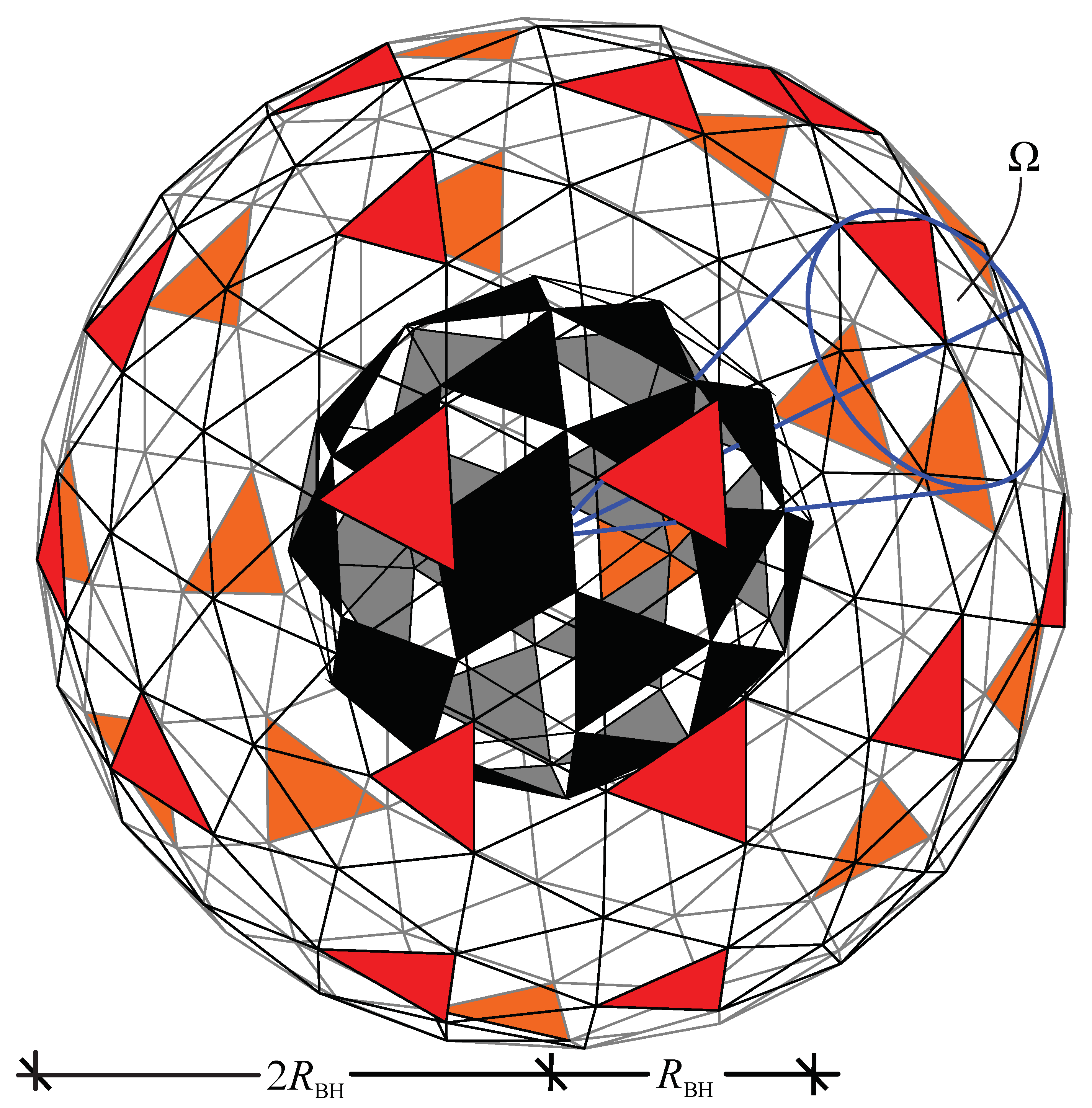
Figure 6.
Lower (red) and upper (green) bound on the number of APTs on a VS as a function of the information capacity of the generating BB [9].
Figure 6.
Lower (red) and upper (green) bound on the number of APTs on a VS as a function of the information capacity of the generating BB [9].
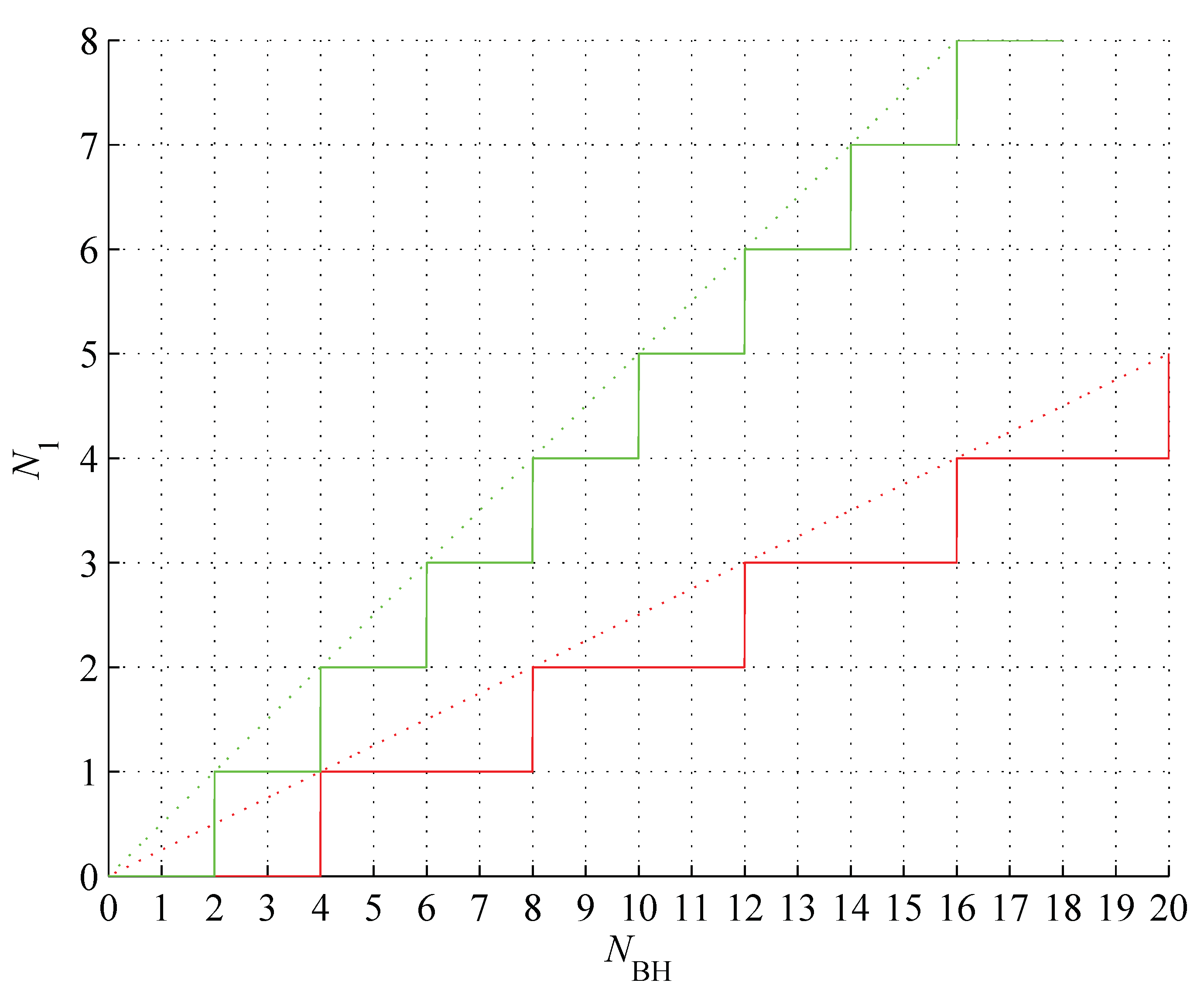
Figure 7.
Lower (red) and upper (green) bounds on and lower (blue) and upper (cyan) bounds on as a function of l defining VS. Characteristic velocities are , .
Figure 7.
Lower (red) and upper (green) bounds on and lower (blue) and upper (cyan) bounds on as a function of l defining VS. Characteristic velocities are , .
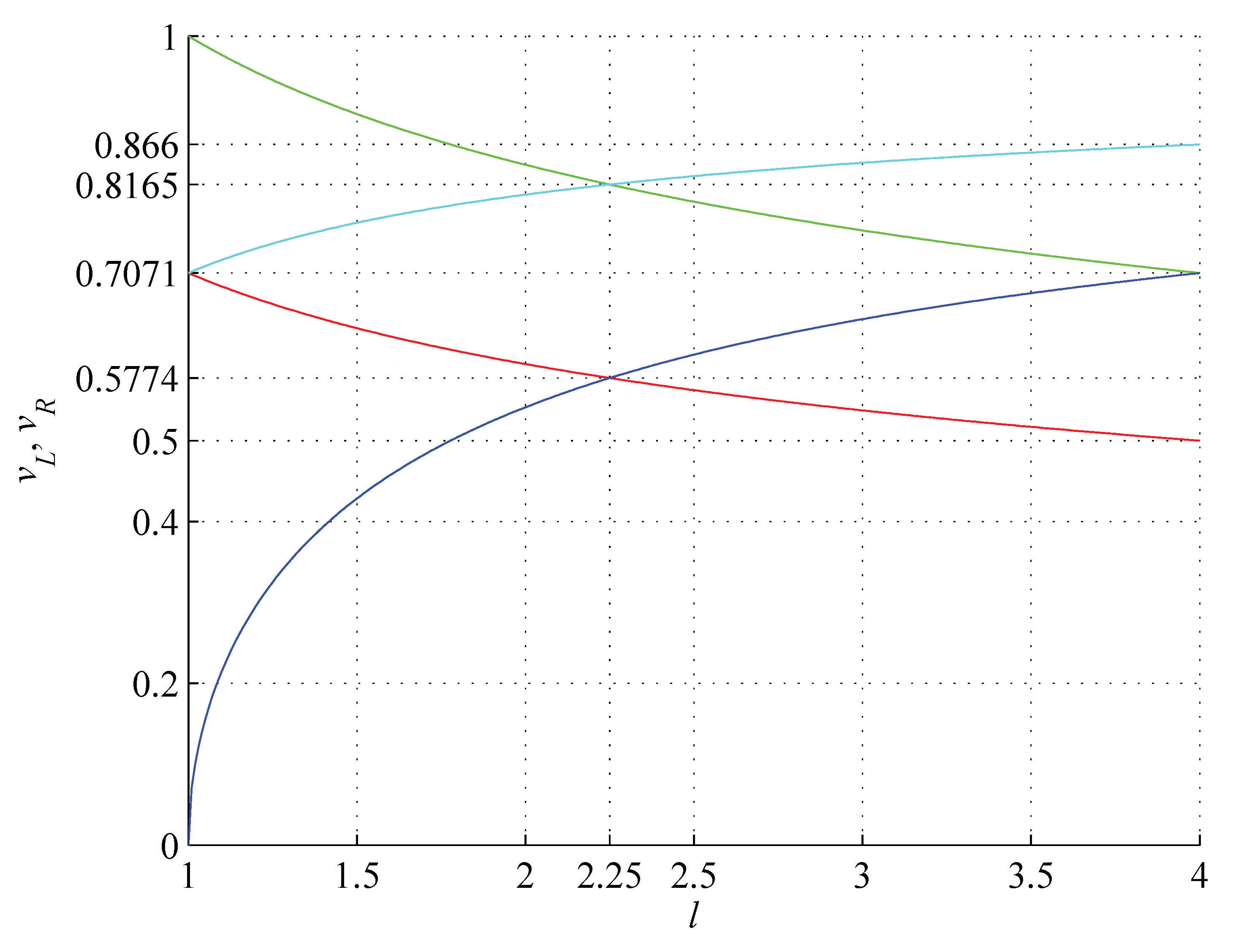
Figure 8.
Lower (red) and upper (green) bounds on the binary string assembly index of length and (blue), for .
Figure 8.
Lower (red) and upper (green) bounds on the binary string assembly index of length and (blue), for .
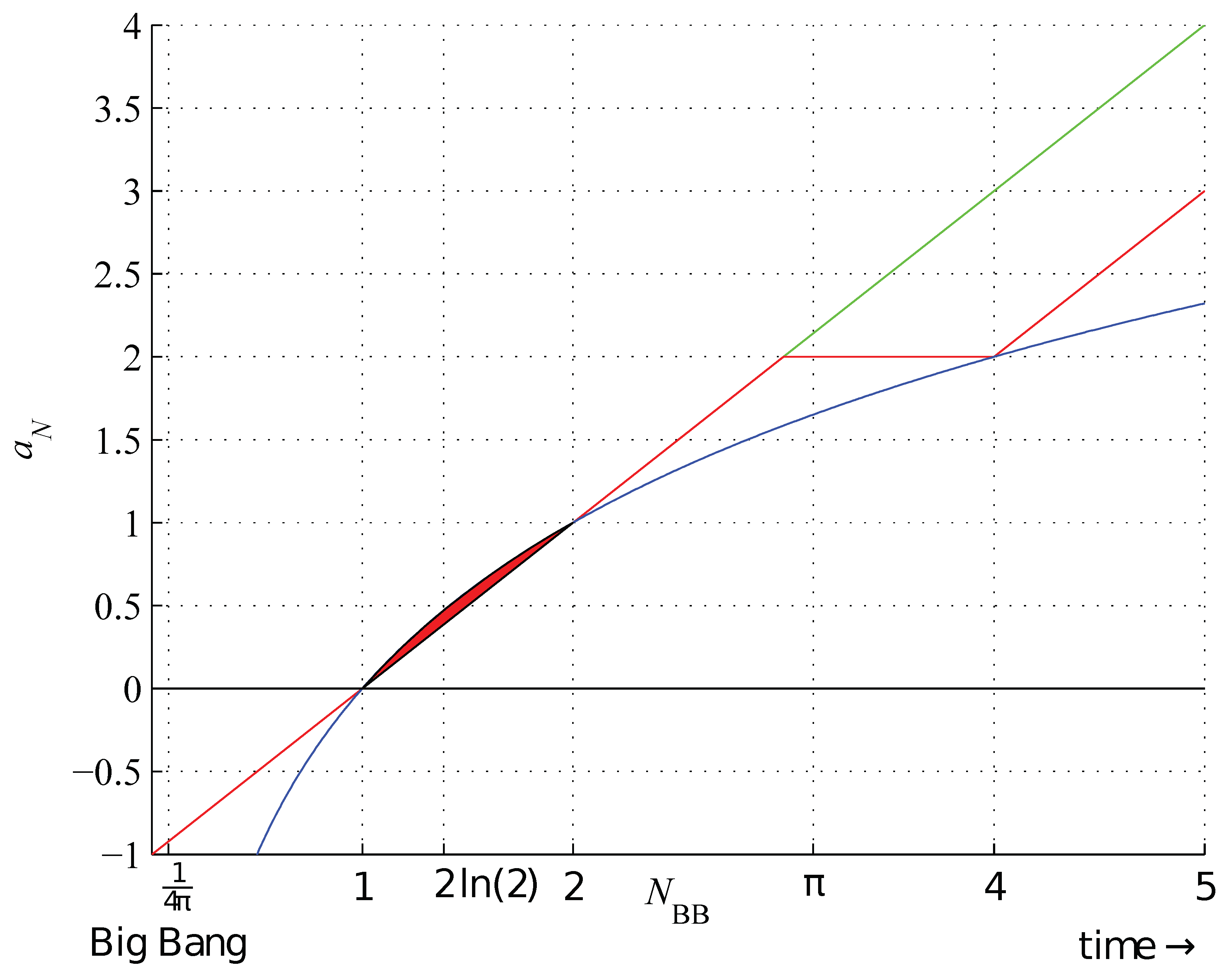
Figure 9.
Black body object energy (green); temperature (red), (red, dash-dot), (red, dash); and work (blue), (blue, dash-dot), (blue, dash),as a function of its information capacity in terms of Planck units, for .
Figure 9.
Black body object energy (green); temperature (red), (red, dash-dot), (red, dash); and work (blue), (blue, dash-dot), (blue, dash),as a function of its information capacity in terms of Planck units, for .
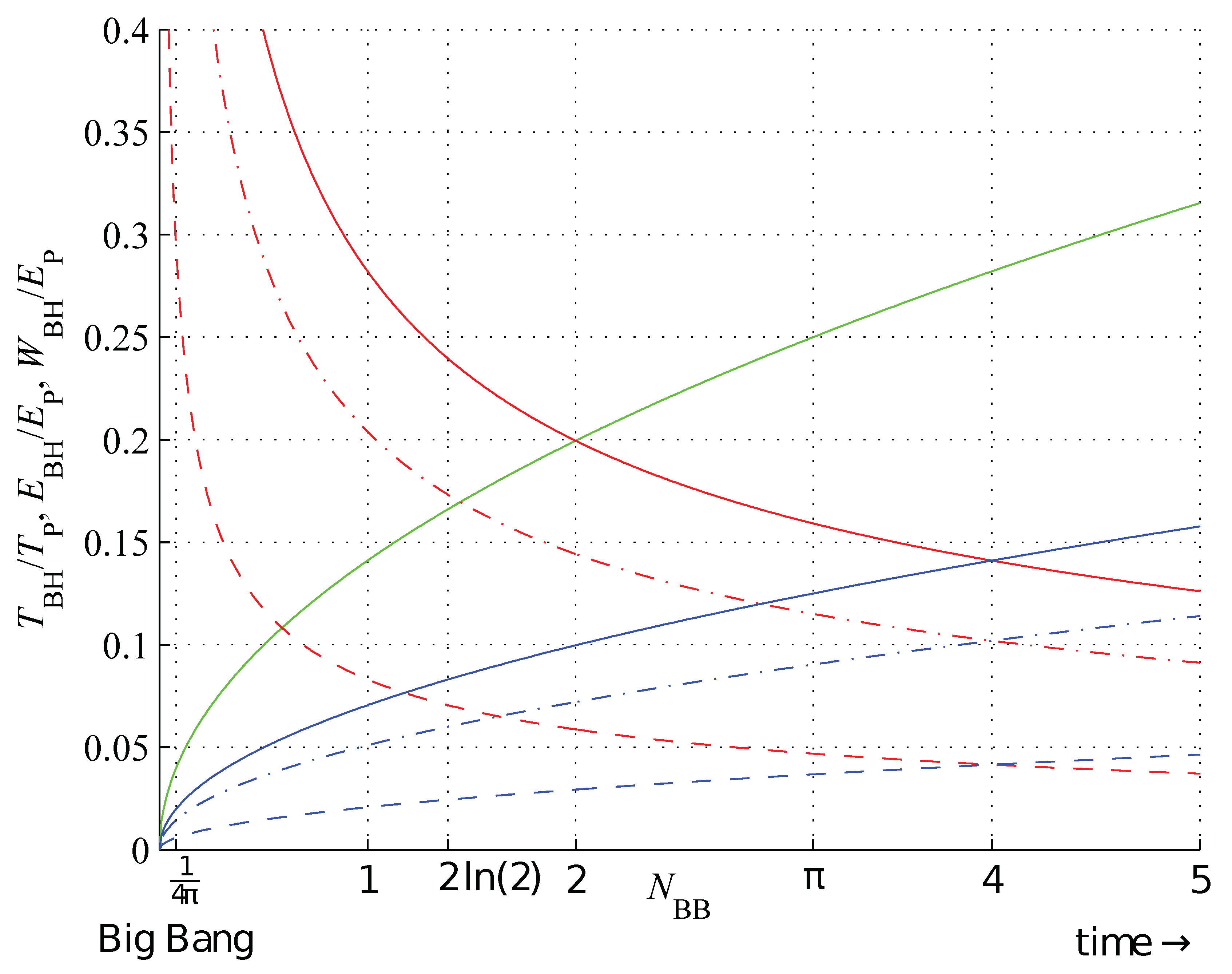
Table 1.
Distribution of the assembly indices for .
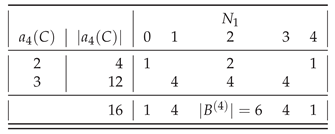 |
Table 2.
balanced strings .
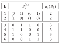 |
Table 3.
2-bit elegant programs producing strings with .
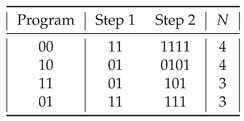 |
Table 4.
3-bit elegant programs assembling strings with .
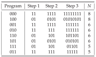 |
Table 5.
4-bit programs assembling strings with .
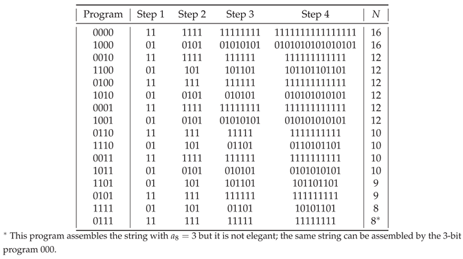 |
Table 6.
String length N, number of all strings , number of balanced strings , number of distinct strings , number of balanced distinct strings , and lower bound on the string assembly index.
Table 6.
String length N, number of all strings , number of balanced strings , number of distinct strings , number of balanced distinct strings , and lower bound on the string assembly index.
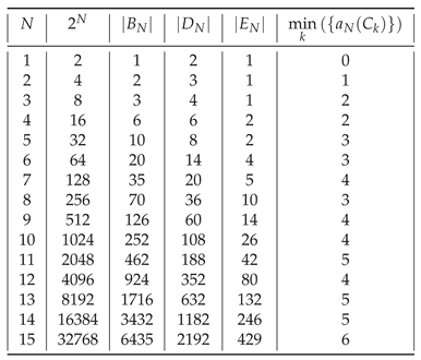 |
Table 7.
Distribution of assembly indices among balanced distinct strings for .
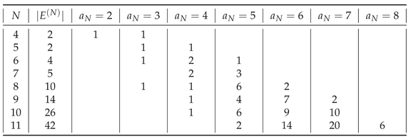 |
Table 8.
Exemplary balanced strings having a maximum assembly index. Conjectured () form of the maximum assembly index and its factual values for distinct () and non-distinct () strings (red if below the conjectured value, green - if above).
Table 8.
Exemplary balanced strings having a maximum assembly index. Conjectured () form of the maximum assembly index and its factual values for distinct () and non-distinct () strings (red if below the conjectured value, green - if above).
 |
Disclaimer/Publisher’s Note: The statements, opinions and data contained in all publications are solely those of the individual author(s) and contributor(s) and not of MDPI and/or the editor(s). MDPI and/or the editor(s) disclaim responsibility for any injury to people or property resulting from any ideas, methods, instructions or products referred to in the content. |
© 2024 by the authors. Licensee MDPI, Basel, Switzerland. This article is an open access article distributed under the terms and conditions of the Creative Commons Attribution (CC BY) license (http://creativecommons.org/licenses/by/4.0/).
Copyright: This open access article is published under a Creative Commons CC BY 4.0 license, which permit the free download, distribution, and reuse, provided that the author and preprint are cited in any reuse.


