
Submitted:
08 January 2024
Posted:
09 January 2024
You are already at the latest version
Abstract
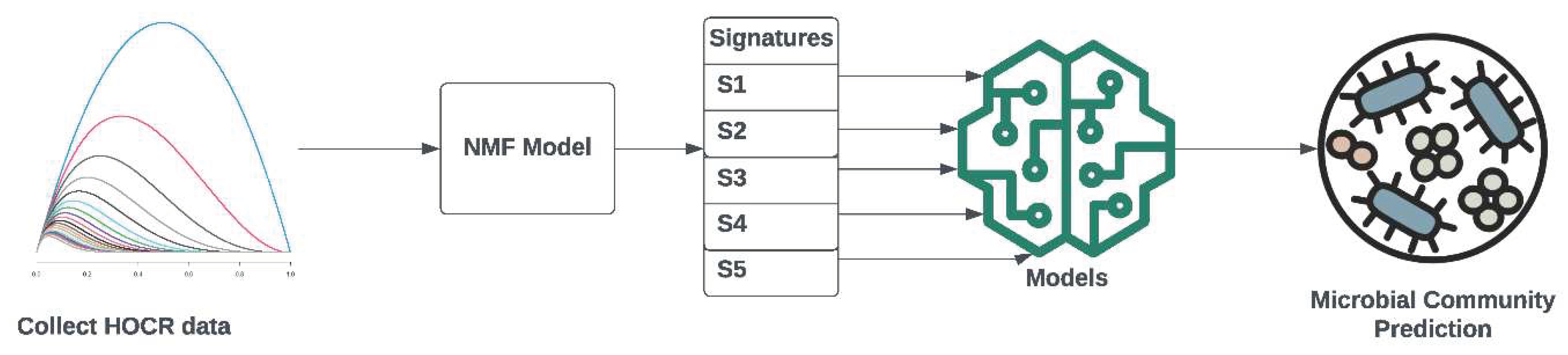
In this communication, we present an innovative approach leveraging advanced Machine Learning (ML) and Artificial Intelligence (AI) techniques, specifically the Non-Negative Matrix Factorization (NMF) method, to analyze downward and upward light spectra collected by Hyperspectral Ocean Color Radiometer (HyperOCR, HOCR) sensors in the water column. Our work focuses on the development of a robust and efficient tool for unraveling the structure and activities of natural microbial assemblages in the ocean. By applying the NMF method to HyperOCR data, we successfully extracted five spectral signatures, representing unique patterns in the data. These signatures were instrumental in predicting the abundances of various microbial components, including bacteria, heterotrophic nanoflagellates, and picoeukaryotes, showcasing the potential of ML and AI in advancing oceanographic studies. To validate the methods, the study area included a shallow coastal area under the influence of freshwater inflow and an open offshore area with a depth of 100 m. The study sites in coastal and offshore waters (Kaštela Bay and Stončica Vis, respectively) had significantly different hydrographic and microbiological characteristics. Kaštela Bay had lower temperatures and salinity than the site on Vis. We have proved by application of different AI and ML methods with specific HOCR sensors prediction of the structure of the microbial community.
Keywords:
spectral signatures
; machine learning
; artificial intelligence
; non-negative matrix factorization
; prediction
; microbial community structure
; ocean
1. Introduction
The implications of global warming on ocean ecosystems necessitate more detailed insights, and traditional approaches fall short in providing the required temporal and spatial resolutions. Here, we employ ML protocols, specifically NMF, to analyze spectral changes in the water column, as measured by HyperOCR sensors. These sensors capture the adsorption and reflection of light, offering a comprehensive view of the water column. Our objective is to explore the wealth of information that can be gleaned by correlating spectral changes with various environmental parameters, thus highlighting the pivotal role of ML and AI in enhancing our understanding of ocean dynamics. Consequences of present global warming trends include pronounced ocean stratification, geographical shifts, and a decrease in nutrient supply with phytoplankton community shifts towards small phytoplankton. Increased concentrations of atmospheric CO2 enhance ocean acidification [1]. Small phytoplankton might find preferable conditions in the interstices of such organic patches balancing the gap in the reduced production as a consequence of warming and acidification.
We applied NMF protocols [2] in analyzing spectral changes of light in the water column as a new tool in oceanography. For understanding primary production in the oceans, it is essential to collect much more detailed information with emerging technologies on both temporal and spatial scales, which is impossible with traditional approaches. That is the reason why we wanted to explore the amount of information we can get from analyzing spectral changes in the water column and correlating them to other measured parameters, as vertical profiles of HyperOCR downward and upward sensors measure adsorption of light and reflection of light throughout the water column respectively, thus providing a very detailed picture of changes in the water column.
The synergy of AI and oceanography illustrates the potential for technological advancements to address environmental challenges. ML algorithms serve as a bridge, connecting intricate sensor data with meaningful insights, paving the way for a new era in oceanographic research.
2. Materials and Methods
In the realm of scientific methodologies, the infusion of ML methodologies stands as a testament to the symbiotic relationship between AI and domain-specific research. The development of models such as NMF amplifies the precision of data analysis, showcasing the capacity of AI to contribute significantly to advancing scientific discovery. Our study, conducted in the central Adriatic Sea, integrates ML techniques into the analysis of data collected through advanced sensor systems. The NMF model, developed using a training dataset of 5397 HOCR curves, successfully extracts five spectral signatures, each revealing distinct patterns across the visible spectrum. These signatures demonstrate unique associations with depth, sensor type (downwelling or upwelling), and environmental parameters, underscoring the versatility of ML in discerning complex patterns in oceanographic data.
2.1. Sampling and incubations
This study was conducted on 12 and 13 June 2023 in the central Adriatic Sea in the vicinity of Split and Vis, Croatia, at a site in Kaštela Bay (12 June, 43⁰ 31’ 33.9’’ N, 16⁰ 23’ 17.6’’ E, depth 38.4 m) and near Stončica lighthouse on Vis Island (13 June, 43⁰ 03’ 32.8’’ N, 16⁰ 17’ 19.7’’ E, depth 102.9 m). Sampling depths in Kaštela Bay were 0, 5, 10, 15, 20, 25, and 28m (K0, K5, K10, K15, K20, K25, K28) and at Stončica - Vis station, the water column was sampled at 0, 5, 10, 20, 30, 50, and 100 m (V0, V5, V10, V20, V30, V50, V100). All samples were taken at predetermined depths by a 5 L Niskin water sampler. Before subsampling, all bottles were rinsed three times with seawater from the sampler.
2.2. Fluorometric determination of chlorophyll and radiometric determination of chlorophyll absorbance spectra
Five hundred (500) mL samples were filtered on 45 mm GF/F glass fiber filters, folded in half, and stored at -20℃ until chlorophyll extraction in the onshore lab. Upon arrival at the laboratory (within 48 hours), the filters were ground in a few mL of 90 % acetone in a glass homogenizer with a motor-driven Teflon pestle, for 1 minute, in an ice bath and under subdued light. After grinding, the extract was carefully transferred to a stoppered and graduated centrifuge tube. The glass homogenizer and the pestle were rinsed with 90 % acetone and the rinsed volumes were added to the centrifuge tube. The extract volume in the centrifuge tube comprised exactly 10 mL of 90 % acetone. Immediately before measurement, the extracts were thoroughly mixed and centrifuged for 10 minutes at 500×g. The fluorometer was calibrated by using a commercial solution of pure chlorophyll a (Sigma-Aldrich C5733 Chlorophyll a). Sample extracts were transferred from the centrifuge tubes to the fluorometer cuvette by careful decanting. The fluorescence of the sample extract was measured against a 90 % acetone blank. After measurements, 0.2 mL 1 % v/v hydrochloric acid was added to the cuvette and mixed. After 2-5 min., the fluorescence of the sample extract was measured again against a 90 % acetone blank. The concentration of Chlorophyll a and phaeopigments was calculated according to the equations of Holm-Hansen et al. [3].
After fluorescence measurements a 3 mL aliquot of the chlorophyll extract was transferred to an optical-grade 10 mm analysis cell to measure light absorbance spectra using Apogee SP-200 spectroradiometer.
2.3. Flow cytometry
For the flow cytometry count of autotrophic cells, 2 mL of preserved samples in 0.5% glutaraldehyde were frozen at -80 °C and stored until analysis on a Cytoflex cytometer (with laser 488 nm, flow rate of 60 µL/min for 200 sec). Autotrophic cells were divided into groups: Synechococcus, Prochlorococcus, and picoeukaryotes, distinguished according to light scattering, red emission of cellular chlorophyll content, and orange emission of phycoerythrin-rich cells. Abundances of Sybr Green-I-stained bacteria, High nucleic acid content (HNA) bacteria, Low nucleic acid content (LNA) bacteria, and heterotrophic nanoflagellates (HNF) were also determined using flow cytometry [4] and the samples were preserved in 2% formaldehyde and stored at 4 °C until analysis.
2.4. Light microscopy
Identification and abundance of phytoplankton communities have been determined using the Utermöhl sedimentation method [5]. Water samples of 250 mL were collected using Nansen bottles and then preserved by adding formaldehyde to achieve a final concentration of 2% formaldehyde-seawater solution. After this preservation, subsamples of 25 ml each were stored in counting chambers for 24 hours. For subsequent analysis, two transects within the sedimentation chamber were selected for counting, which was facilitated by an inverted microscope. The choice of magnification, either ×200 or ×400, was based on the size of the species being observed.
2.5. Solar radiation, salinity, temperature, and depth measurements
In this study, we used two vertical profilers and a reference hyperspectral curve station. The first vertical profiler (SBE 25plus Sealogger CTD) measured conductivity, temperature, and depth profiles. The second vertical profiler measured downward and upward irradiance profiles with two Hyperspectral Ocean Color Radiometer (HOCR) (Seabird) sensors calibrated for measurements of downwelling and upwelling radiation with optical data in the range from 350-1200 nm (extended range). HOCR sensors were mounted on a frame equipped with an SBE 39plus temperature (external thermistor), depth (100 m strain gauge pressure sensor), and time sensors. Measured data were recorded in a custom-built data logger built by MARINIX Ocean Tech. The third part of this system was a hyperspectral color radiometer sensor (Apogee PS-200 laboratory hyperspectral radiometer, 300-850 nm range, 0.5 nm sensitivity) that was installed on the highest point on the vessel with the sensor pointed upwards vertically to measure reference surface light spectra during the vertical profile casts of the water column with HOCR.
2.6. Preprocessing of hyperspectral curves using reference measurements
On both stations (Kaštela and Vis), we utilized multiple sensor systems for data collection. The purpose of Apogee HOCR, positioned on the highest point on the vessel, was to collect HOCR curves representing reference data (at a particular time point) that can be paired with vertical profiler data. The reference curve was then used to normalize the data from the vertical profiler, resulting in curves whose values range from 0 to 100, representing the percentage of the reference curve at a certain nanometer.
2.7. Computational Requirements
All model training, genetic algorithm, and NMF were run in Python on regular laptop with the following specifications: Lenovo IdeaPad 3 - 17ITL6 laptop type 82H9, 17-inch, 11th Generation Intel Core i5 - 1135G7, Intel iRIS graphics, memory 2 x 8 GB DDR4-3200, hard drive 512 GB SSD PCIe.
3. Results
Our findings showcase the ML-based model's efficacy in predicting microbial community structures. By applying the extracted spectral signatures, we achieve minimal root mean square error (RMSE) in predicting bacteria, heterotrophic nanoflagellates, and picoeukaryotes. Notably, ML predictions exhibit intermediate RMSE values for Prochlorococcus and larger RMSE for Synechococcus and HNA bacteria, shedding light on the varying predictability across different microbial components.
3.1. Hydrographic properties of the water column
To characterize the study sites, we examined the differences in thermohaline properties at the study sites in Kaštela Bay and Stončica - Vis. The onset of seasonal stratification was observed in both vertical temperature profiles, with a warmer layer at the top and a colder one at the bottom. This is due to surface warming and relatively weak wind forcing during the warm period of the year (July to September)[6].Both salinity and temperature were lower in Kaštela Bay than in Stončica-Vis (oligotrophic site in the open sea), indicating the different characteristics of the two studied sites (Figure A1). Since Kaštela Bay of Kaštela is surrounded by urban development and intense human activity (near the port of Split), with a significant freshwater discharge of the river Jadro (average annual inflow of ~ l0 m3 s-1) and several submarine sources of lower intensity, it can be assumed that these have an influence on the hydrographic characteristics of the seawater body [6].
3.2. Developing HOCR signatures using a non-negative factorization model on training data
Using our custom-built vertical profiler and prior to the experiment, we collected HOCR curves at different locations in the southern Adriatic Sea in the vicinity of the Island of Mljet, and at different time points of the day. This resulted in a dataset containing 5397 HOCR curves which we used as a training dataset for model development. The model we developed is based on the Non-Negative Matrix Factorization method (NMF) [7,8], which uses the input data (HOCR) curves in order to factorize them into two matrices. The first matrix (H) represents “spectral signatures”, which are unique patterns in the data discovered by the method. The second matrix (W) represents the weights of each curve (sample) towards each signature. To determine the optimal number of signatures in the data, we applied NMF multiple times with different numbers of signatures (2 to 10), measuring reconstruction error. The reconstruction error was measured using two methods (Frobenius Norm and Kullback-Leibler) [9] and resulted in an optimal number of signatures K = 5 (Figure 1a).
Once the optimal number of signatures was found, we fitted the model using the training data and the following hyperparameters: n_components = 5, init='nndsvda', solver='cd', beta_loss='frobenius', max_iter=10000. The model successfully extracted five spectral signatures (S1-S5), representing distinct patterns in the data. S1 showed the highest peak at 359 nm, followed by the peak at 597 nm (Figure 1b, blue curve). S2 showed a single peak at 506 nm (Figure 1b, orange curve). S3 was characterized with a similar curve as S2, however, with a smaller peak at 490 nm (Figure 1b, green curve). S4 captured a wide spectrum range from 350 nm to 580 nm in an almost uniform fashion (Figure 1b, red curve). S5 is characterized by a spectral curve spanning from 350 nm to 560 nm, having two peaks at 393 nm and 496 nm (Figure 1b, purple curve). Since the training data contained the HOCR curves coming from downward (DW - downwelling radiation) and upward (UW - upwelling radiation) sensors, we compared the extracted signatures between those two sensors. Downward (DW) sensor data is mostly characterized by S3, followed by S5, whereas upwelling sensor data showed more complex distribution of signature enrichment (Figure 1c). Next, we computed kernel density estimation (KDE) for a probability density between signature enrichment and depth. We visualized the KDE for each signature-depth pair and observed that S1 extracted from the DW sensor shows a linear correlation towards depth where DW shows enriched density around depth 0 and 100 meters. Spectral signature S2 extracted from the UW sensor showed almost no patterns with respect to depth, however, most of the enrichment is located around 20 m depth. S3 extracted from the DW sensor shows a linear pattern with respect to depth with increased density between 0 and 40 meters depth whereas S3 extracted from UW shows increased density around 90 m depth. S4 extracted from UW curves showed limited density, whereas signature S4 extracted from DW curves showed increased density across the entire measured water column (0-100 m), particularly around 10 meters depth. S5 extracted from UW curves shows a negative linear pattern with respect to depth and increased density around 90 meters depth. S5 extracted from the DW HOCR curve showed increased density throughout the entire measured water column (0-100 m) with an increase in density of around 20 meters of depth (Figure 1d). Finally, extracted five spectral signatures show unique patterns, capturing complex patterns across the entire visible spectrum, indicating differences between UW and DW sensors, and showing association to depth. The summary of signature characteristics can be found in Table 1.
3.3. HOCR spectral signatures at study locations
We measured seven HOCR profiles at two investigated stations, Kaštela Bay and Stončica - Vis. From HOCR profiles we extracted 5 spectral signatures. Signature S1 had strong peaks at 363 nm and 580 nm, upwelling (UW) signature had positive correlation with depth while downwelling (DW) signature S1 was present at 0 m and a little at 100 m. Signature S2 had a strong peak at 503 nm with no presence in UW profiles while DW signature was present throughout the water column with maximum occurrence at 20 m. UW signature S3 with peak at 493 nm showed negative correlation with depth and was most abundant at 40 and 90 m. DW signature S3 had positive correlation with depth with maximum from 0 m to 40 m. The Signature S4 had a small uniform curve from 350 nm to 550 nm. DW signature was either abundant from 0 m to 20 m or not present at all. UW signature S4 showed modest presence at 90 m. Signature S5 was similar to S4 (350 nm to 520 nm) with a more pronounced peak. DW signature was present in all profiles and depths while UW signature was negatively correlated with depth with maximum at 80 m. DW profiles were dominated with signatures S3 and S5, almost no S1. UW profiles were dominated with signature S4 and a little bit less with S3, S5 and S1. Signature S2 was not present.
3.4. Microbial community structure at the two stations
We assessed the community structure and count of the microbial community with a flow cytometer and Utermöhl counting method [10]. Overall, the community is dominated by cyanobacteria Synechococcus (concentrations ranging from 22.60 x 10³ to 30.50 x 10³ cells/mL at Kaštela and 2.00 x 10³ to 13.60 x 10³ cells/mL and Stončica - Vis location) with the highest concentrations at the surface decreasing with depth at Kaštela and highest concentrations at 30 m and 50 m at Stončica - Vis location. Cyanobacterium Prochlorococcus (concentrations ranging from 1.39 x 10³ to 6.07 x 10³ cells/mL at Kaštela and 0.70 x 10³ to 33.00 x 10³ cells/mL and Stončica - Vis location) had the lowest concentrations at the surface with increasing concentrations with depth, exhibiting dominant concentrations (14.27 x 10³ and 33.00 x 10³ cells/mL) at 50 m and 100 m, respectively at Stončica - Vis oligotrophic location. Picoeukaryotes concentrations generally decreased with depth, with a slight increase at 30 m at Kaštela location (concentrations ranging from 0.86 x 10³ to 3.37 x 10³ cells/mL) and were higher at 0m and 5m than the rest of the water column where the concentrations were uniform at Stončica - Vis location (concentrations ranging from 0.57 x 10³ to 1.56 x 10³ cells/mL). Concentrations of heterotrophic nanoflagellates were uniform throughout the water columns at both Kaštela and Stončica - Vis locations (concentrations ranging from 0.13 x 10³ to 0.40 x 10³ cells/mL). Heterotrophic bacteria were the most dominant population within the microbial community at both locations, uniformly distributed throughout the water columns (concentrations ranging from 0.31 x 10⁶ to 0.55 x 10⁶ cells/mL at Kaštela and 0.15 x 10⁶ to 0.30 x 10⁶ cells/mL and Stončica - Vis location). The density and enrichment of Prochlorococcus, Synechococcus, and picoeukaryotes in the water column is shown in Figure A4.
3.5. Fitting the model on independent data collected at two stations
After model training, we used the trained NMF model on data obtained at Kaštela (K0, K5, K10, K15, K20, K25, K28) and Stončica - Vis (V0, V5, V10, V20, V30, V50, V100). First, we inspected the signature enrichment distribution between the two locations and two sensors (downwelling and upwelling). At Kaštela Bay, downwelling-sensor (DW) (Figure 2a, left top), we observed a dominant presence of S1 and S3. S1 starts the highest and peaks at 0 m, peaks at 5 m, and slowly vanishes.
Furthermore, S1 was also correlated (r = 0.87 P < 0.001) to Synechococcus, Heterotrophic nanoflagellates, and Picoeukaryotes count (Figure 2b, Kaštela Downwelling panel) and spectral peaks of 356 nm and 593 nm. Enrichment of S3 was expressed in two peaks, one at 5 m and another one at 28m. Furthermore, S3 (curve peak at 496 nm) showed a significant positive correlation to Chlorophyll a and Prochlorococcus (r = 0.71 P < 0.001 and r = 0.72, P < 0.001) (Figure 2b, Kaštela Downwelling panel). Signatures S2 and S5 showed similar patterns as they started with low values, peaked at 10m, and decreased afterward. At the same location and in the upwelling sensor (UW) (Figure 2a, right top), we observed a dominant presence of S3 and S1 with limited enrichment of S4 at 5, 10, and 15m. The signature S1 (curve peaks at 356 nm and 597 nm) is also correlated with Chlorophyll a, Prochlorococcus, and Picoeukaryotes (r = 0.48, P < 0.001; r = 0.38, P < 0.001; r = 0.57, P <0.001) (Figure 2b, Kaštela upwelling panel) indicating different community structures at the surface compared to the lower parts of the water column. S1 showed the highest enrichment at 0 and 28 meters and the lowest at 10m. At Stončica - Vis station DW, we observed almost no presence of S2 and some level of enrichment in other signatures. Signature S4 started with low values, peaked at 20 m, and decreased as depth increased. Signature S1 showed the highest enrichment at the surface and decreased as depth increased, except for 100m (Figure 2a, Stončica - Vis DW panel). Signature S3 showed enrichment at all depths, reaching a maximum at 50 m. Looking at the UW sensor at the same location, we observed no presence of S4 except for 0 meters. S4 was also characterized with a strong positive correlation (r = 0.48, P < 0.001; r = 0.6 P < 0.001) towards Chlorophyll a and Prochlorococcus (Figure 2b, Stončica - Vis UW panel). Signature S5 (wide curve with a peak in 446 nm) showed dominant enrichment peaking at 5 m and 20 m. Signature S3 showed maximum enrichment at 0m and 30m and a strong correlation (r = 0.79, P < 0.001; r = 0.72, P < 0.001; r = 0.81, P < 0.001) with Synechococcus, Bacteria, and Heterotrophic nanoflagellates (Figure 2b, Stončica - Vis UW panel). Next, we calculated and analyzed the Chlorophyll a absorbance for both stations (Kaštela and Stončica - Vis). At the Kaštela station, we observed the highest absorbance at 30 m and minimum absorbance at 5m depth, whereas at Stončica - Vis station, the highest absorbance was measured at 0m and minimum at 100 m depth (Figure 2c). Interestingly, the second highest chlorophyll absorbance at Stončica - Vis station was at 30 m depth, where absorbance in the spectrum of 400 to 500 nm exceeded the absorbance of 0m. Furthermore, V30 is also characterized by enriched S4 (DW), which is characterized by a broad, low-intensity curve located between 353 and 503 nm and an increased concentration of Prochlorococcus.
Finally, we inspected the overall association of the count (103 cell/mL) of members of the picoplankton community and depth. Synechococcus count was significantly negatively correlated (r = -0.51, P = 0.008) with depth (m), and Prochlorococcus was significantly positively correlated (r = 0.95, P < 0.001) with depth (m) (Figure A2).
3.6. Phytoplankton abundance and community structure
At both locations, phytoplankton abundance was measured in order to assess the community structure. Kaštela Bay water column was dominated by diatoms, having almost uniform and enriched abundance at all measured depths (0-30 m) (Figure 3a).
In contrast, silicoflagellates showed no presence at both stations except for Kaštela - 30m. In Kaštela, the surface was largely dominated by diatoms, whereas at Stončica - Vis, dinoflagellates were the most abundant (Figure 3b). At Stončica - Vis, diatoms show an interesting pattern where they start at a high value at the surface, reaching a minimum at 20 m and then again steadily increasing and reaching a maximum at 100 m. The similar pattern we observed for S1 for both UW and DW sensors at Stončica - Vis (Figure 2a) suggests an association between diatom abundance and S1. To further investigate this, we correlated signatures to phytoplankton groups and observed positive correlations between S1 and diatoms for Stončica - Vis (Figure 3c, Figure A3). Furthermore, at Kaštela, nanoflagellates and S4 from the upwelling curve showed a similar pattern reaching a maximum value at 5m and slowly decreasing until 30m (Figure 3a, Figure 2a). This was further confirmed by a correlation coefficient between S4 and nanoflagellates, suggesting a strong positive correlation (Figure 3d, Figure A3). In Kaštela, we also observed that the abundance of coccolithophores started with smaller values at the surface and increased until 10-20m and then decreased, reaching a minimum at 30m (Figure 3a). A similar pattern was observed for S5 (only DW) in Kaštela, where S5 enrichment peaked at 10m (Figure 2a), suggesting an association between S5 (DW) and the abundance of coccolithophores (Figure A3). Performing hierarchical clustering (ward algorithm) on correlation coefficients between phytoplankton and signatures, we observed different community structures between Kaštela and Stončica - Vis locations. At Stončica - Vis location, diatoms were strongly associated with S1 and S2 while negatively associated with S4 and S5 (Figure 3c). At Kaštela, diatoms showed an intermediate association with S1 and a strong negative association with S4 (Figure 3d). Lastly, we correlated Chlorophyll a and PPP with the abundance of phytoplankton groups. We observed a significant positive correlation between the abundance of diatoms and Chlorophyll a (r = 0.75 P = 0.02) and a marginally significant negative correlation (r = -0.66 P = 0.052) between coccolithophores and Chlorophyll a (Figure 3e).
Abundances and detailed species distribution per station per depth are shown in Supplementary Data File.
3.7. Spectral signatures and microbial community structure
The collected data for microbial community structure and HOCR can be paired by depths which is ideal for modeling. For this purpose, we constructed simple linear regressions to predict count (103 Cells/mL) using our signatures (S1 - S5) and depth. For each microbial count, we made a model using extracted signatures from the upwelling curve and the downwelling curve. Next, we plotted the observed count (103 Cells/mL) on the x-axis and the predicted count (103 Cells/mL) on the y-axis. In the ideal case, those points would form a diagonal line representing no difference between observed and predicted values. This analysis showed that bacteria, heterotrophic nanoflagellates, and picoeukaryotes can be predicted using extracted signatures with minimal root mean square error (RMSE), where Prochlorococcus showed intermediate RMSE values and finally, Synechococcus and HNA bacteria showed large RMSE (Figure 4a-f).
When predicting bacteria, we observed an RMSE of 0.08 when using a downwelling curve and RMSE = 0.06 when using an upwelling curve, indicating that bacterial count can be effectively estimated using our signatures. The coefficient associated with the depth is equal to zero, indicating that all information for prediction is coming from signatures, mainly from S2, when looking at the downwelling curve model (Figure 4b). Fitting a model that predicts the count of heterotrophic nanoflagellates showed the best results in terms of RMSE. We calculated RMSE of 0.04 when using the downwelling curve and RMSE of = 0.06 when using the upwelling curve (Figure 4c). The model that predicts Picoeukaryotes showed an RMSE of 0.39 when using signatures from the downwelling curve and an RMSE of 0.40 when using signatures from the upwelling curve. The coefficient of 0.03 associated with depth indicates a minor association of depth with count (Figure 4d). Fitting a model that predicts the count of Prochlorococcus, we observed an RMSE of 1.27 when using signatures extracted from the downwelling curve and an RMSE of 0.89 when using signatures extracted from the upwelling curve. We observed a positive coefficient (0.36 for downwelling and 0.23 for upwelling) associated with depth (Figure 4e) which follows the previous finding of an overall positive correlation between Prochlorococcus count and depth (Figure A2). The model that predicts the count of Synechococcus achieved poor results in terms of RMSE. When using extracted signatures from the downwelling and upwelling curves, we calculated an RMSE of 4.54 and an RMSE of 2.50, respectively (Figure 4f). Interestingly, coefficients associated with signatures vary when using downwelling and upwelling curves for signature extraction but also when comparing different species. In Kaštela, when using downwelling sensor signatures, we observed that heterotrophic nanoflagellates were strongly correlated with S1 (characterized by HOCR peaks at 363 nm and 583 nm) that was enriched at 0 m and 5 m depths (Figure 2b). In Stončica - Vis, when using an upwelling curve for signature extraction, we observed that the count of bacteria was strongly correlated with S3, which is characterized by a small peak in 483 nm in a HOCR curve. When looking at the S3 enrichment (Figure 2a, Stončica - Vis UW), we observed that S3 showed high enrichment at a depth of zero, minimal enrichment at 5 m,10 m, and 20 m depths, and again high enrichment at 30 m and 50 m depth, indicating a complex structure of the microbial community and their interaction with light spectrum.
4. Discussion
The outcomes of our study underscore the potential of AI to enhance predictive modeling in ecological studies. The nuanced RMSE values reveal the intricacies of microbial predictions, encouraging further exploration into refining ML algorithms for more accurate ecological assessments. The integration of ML and AI components, particularly the NMF model, emerges as a transformative approach for real-time, detailed analysis of ocean water columns. The correlation between spectral signatures and microbial abundances highlights the potential of ML in advancing our understanding of ocean ecosystems. Our results pave the way for a paradigm shift, where sensor systems coupled with AI frameworks enable comprehensive oceanographic analyses without the traditional reliance on water samples.
Measurements of samples taken at specific depths and the extracted signatures provide comprehensive results. Combining all the approaches described above, our results clearly show a significant relationship between the microbial community, photosynthetic and heterotrophic activity, and downwelling and upwelling radiation intensity in the water column. Downwelling irradiance spectra represent adsorption of spectra through the water column by the seawater, inorganic particles, and microbial consortia, while upwelling spectra represent the reflection of spectra from different particles below the upwelling sensor.
Our extracted spectral signatures can accurately predict the numbers of bacteria, heterotrophic nanoflagellates and picoeukaryotes Cyanobacteria (both Prochlorococcus and Syechococcus) are poorly predictable from our Signatures (only associated with depth). HNE is also very poorly predictable regardless of depth (Figure 4). As we reflect on the implications of our findings, the role of AI in shaping the future of oceanography becomes increasingly evident. The marriage of advanced sensors and ML models not only expedites data analysis but also opens avenues for continuous, real-time monitoring of oceanic dynamics, ushering in a new era of AI-driven environmental science. The process of predicting phytoplankton concentrations from measured HOCR spectra is shown in a flow diagram in Figure A5.
We have shown that HOCR extracted spectral signatures can be used to predict the structure of the microbial community. Using extracted spectral signatures with minimal root square error (RMSE), where Prochlorococcus showed intermediate RMSE values and finally, Synechococcus and HNA bacteria showed large RMSE, abundances of bacteria, heterotrophic nanoflagellates, and picoeukaryotes can be predicted. Our results opened a clear pathway towards the concept of ocean water column detailed and comprehensive analysis (from macro to nanometer scales) in real time, using solely sensor systems coupled with AI data analysis framework without the necessity to take seawater samples with bottles.
Author Contributions
Conceptualization, S.P. and K.Y.B.; methodology, S.P. M.S. and K.Y.B.; software, M.S.; validation, S.P., M.S. and K.Y.B.; formal analysis, S.P., M.S. and Ž.N.; investigation, S.P., M.S., Ž.N., D.Š., S.S., T.Dž. and H.P.; resources, S.P. and Ž.N.; data curation, M.S.; writing—original draft preparation, S.P., M.S., Ž.N., D.Š., S.S., T.Dž., H.P., K.Z.B.; writing—review and editing, S.P., M.S. and K.Y.B.; visualization, S.P. and M.S.; supervision, S.P.; project administration, S.P.; funding acquisition, S.P. All authors have read and agreed to the published version of the manuscript.
Supplementary Materials
The following supporting information can be downloaded at the website of this paper posted on Preprints.org.
Author Contributions
Conceptualization, S.P. and K.Y.B.; methodology, S.P. M.S. and K.Y.B.; software, M.S.; validation, S.P., M.S. and K.Y.B.; formal analysis, S.P., M.S. and Ž.N.; investigation, S.P., M.S., Ž.N., D.Š., S.S., T.Dž. and H.P.; resources, S.P. and Ž.N.; data curation, M.S.; writing—original draft preparation, S.P., M.S., Ž.N., D.Š., S.S., T.Dž., H.P., K.Z.B.; writing—review and editing, S.P., M.S. and K.Y.B.; visualization, S.P. and M.S.; supervision, S.P.; project administration, S.P.; funding acquisition, S.P. All authors have read and agreed to the published version of the manuscript.
Funding
This research was funded by Regionale Forskningsfond Agder (RFF Agder), Project number 338390. Development of the new technology used in this study was funded by Innovasjon Norge (Innovation Norway).
Institutional Review Board Statement
Not applicable.
Data Availability Statement
All code for analysis and plotting is available on the public GitHub repository (https://github.com/mxs3203/MarinixExperimentPaper). The GitHub repository provides code for the NMF model, HOCR data processing, figures included in the manuscript, and linear regression fit. The data matrices can be downloaded as supplementary material.
Acknowledgments
We would like to thank the NORCE Norwegian Research Centre for the support and making this study possible, Martin Žagar and Adrián Gómez Repollés for comments on the manuscript.
Conflicts of Interest
The authors declare no conflicts of interest. The funders had no role in the design of the study; in the collection, analyses, or interpretation of data; in the writing of the manuscript; or in the decision to publish the results.
Appendix A
Figure A1.
a. Salinity in the water column as measured during the study at both study locations. b. Temperature in the water column as measured during the study at both study locations.
Figure A1.
a. Salinity in the water column as measured during the study at both study locations. b. Temperature in the water column as measured during the study at both study locations.
Figure A2.
Association of picoplankton species concentrations and depth.
Figure A3.
Heatmaps of correlations between spectral signatures extracted from HOCR measured spectra from UW and DW sensors and dominant phytoplankton groups.
Figure A3.
Heatmaps of correlations between spectral signatures extracted from HOCR measured spectra from UW and DW sensors and dominant phytoplankton groups.
Figure A4.
The density and enrichment of Prochlorococcus, Synechococcus, and picoeukaryotes in the water column.
Figure A4.
The density and enrichment of Prochlorococcus, Synechococcus, and picoeukaryotes in the water column.
Figure A5.
Flow diagram showing the process of predicting phytoplankton concentrations from measured HOCR spectra.
Figure A5.
Flow diagram showing the process of predicting phytoplankton concentrations from measured HOCR spectra.
References
- Marinov, I.; Doney, I.D.; Lima, S.C. Response of ocean phytoplankton community structure to climate change over the 21st century: partitioning the effects of nutrients, temperature and light. Biogeosciences 2010, 7, 3941–3959. [Google Scholar] [CrossRef]
- Puškarić, S.; Sokač, M.; Matić, K. Application of non-negative matrix factorization for studying short-term physiological changes in grapevine from canopy hyperspectral reflection. RIThink 2021, 10, 1–25. [Google Scholar]
- Holm-Hansen, O.; Lorenzen, C.J.; Holmes, R.W.; Strickland, J.D.H. Fluorometric Determination of Chlorophyll. ICES J Mar Sci 1965, 30, 3–15. [Google Scholar] [CrossRef]
- Gasol, J.M.; Morán, X.A.G. Flow cytometric determination of microbial abundances and its use to obtain indices of community structure and relative activity; Springer Protocols Handbooks; Springer: Berlin/Heidelberg, Germany, 2015; pp. 159–187. [Google Scholar]
- Utermöhl, H. Zur Ver vollkommung der quantitativen phytoplankton-methodik. Mitt. - Int. Ver. Theor. Angew. Limnol. 1958, 9, 1–39. [Google Scholar]
- Marasović, I.; Gačić, M.; Kovačević, V.; Krstulović, N.; Kušpilić, G.; Pucher-Petković, T.; Odžak, N.; Šolić, M. Development of the red tide in the Kaštela Bay (Adriatic Sea). Mar Chem 1991, 32, 375–387. [Google Scholar] [CrossRef]
- Lee, D.D.; Seung, H.S. Learning the parts of objects by non-negative matrix factorization. Nature 1999, 401, 788–791. [Google Scholar] [CrossRef] [PubMed]
- Pauca, V.P.; Piper, J.; Plemmons, R.J. Nonnegative matrix factorization for spectral data analysis. Linear Algebra Appl 2006, 416, 29–47. [Google Scholar] [CrossRef]
- Lancaster, P.; Tismenetsky, M. The Theory of Matrices: With Applications, 2nd ed.; Academic Press: Cambridge, Massachusetts, United States, 1985; pp. 1–586. [Google Scholar]
- Paxinos, R. A rapid Utermohl method for estimating algal numbers. J Plankton Res 2000, 22, 2255–2262. [Google Scholar] [CrossRef]
Figure 1.
Signature development using training data. (a) In order to find the optimal number of signatures (K), we computed two measurements (Frobenius norm and Kullbeck-Leibler), for every K in the range of two to ten. This analysis showed that K = 5 is the optimal number of signatures. (b) Each signature can be visualized as a spectral curve indicating distinct patterns in data. (c) Signatures were made using data collected from two sensors, upwelling (UW) and downwelling (DW). The two sensors show distinct enrichment of signatures. (d-h) To investigate association between depth and each signature, we computed the Kernel Density Estimation (KDE). This analysis showed that some signatures are present at all depths (S1, S3, S5) while others are present mostly around surface (S2 and S4).
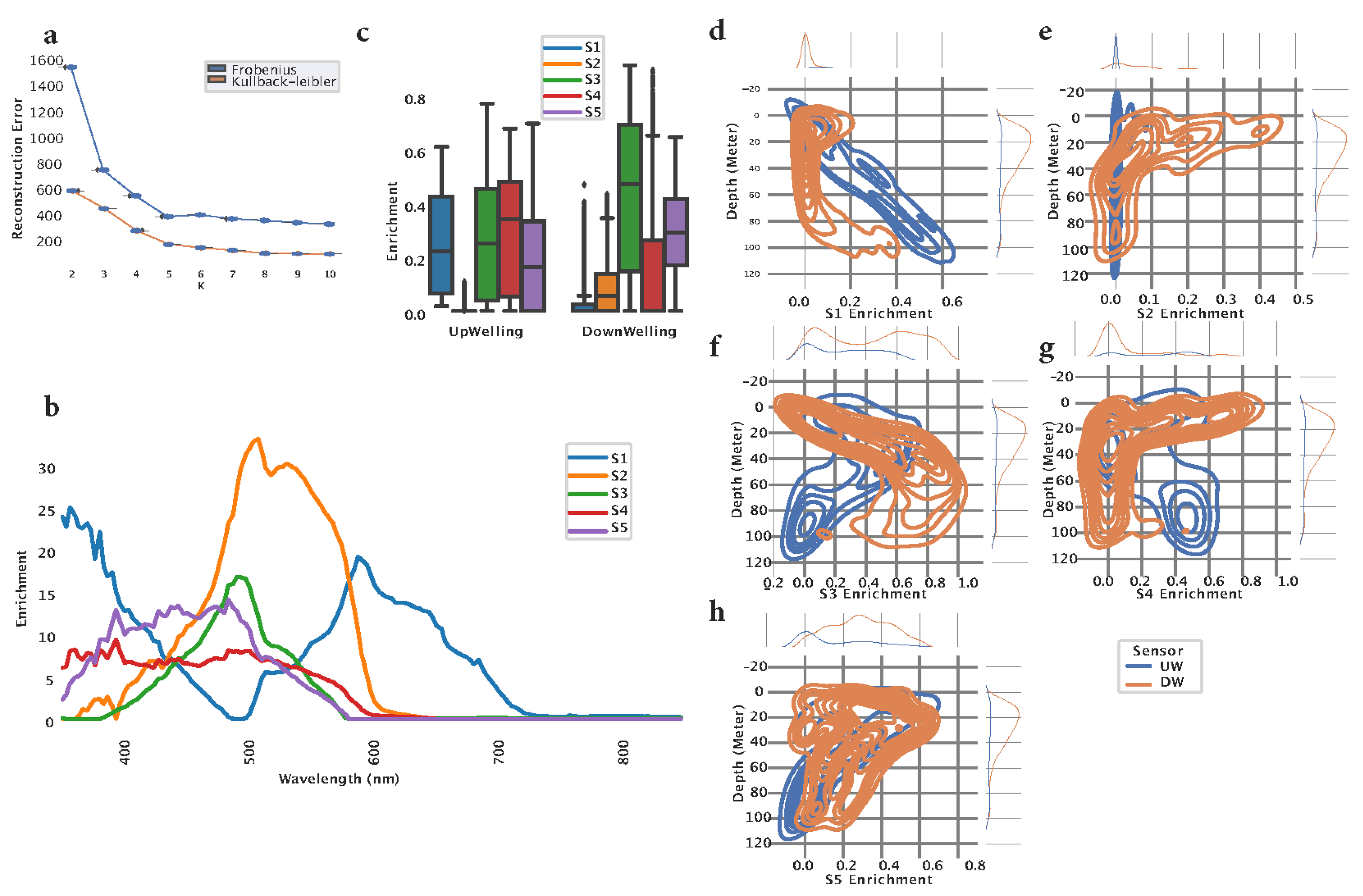
Figure 2.
NMF application of HOCR curves collected at two locations. (a) Trained NMF model was applied on collected data at Kaštela - Bay and Stončica - Vis. The bar plot shows enrichment of each signature for each measurement. (b) The heatmap shows correlation coefficients between signature enrichment and abundance of cyanobacteria, heterotrophic bacteria, heterotrophic nanoflagellates, picoeukaryotes and Chlorophyll a for both locations and both sensors. (c) The line plot shows absorption of Chlorophyll a within the spectrum of 300 nm and 900 nm. The colors indicate the depth where the sample was collected.
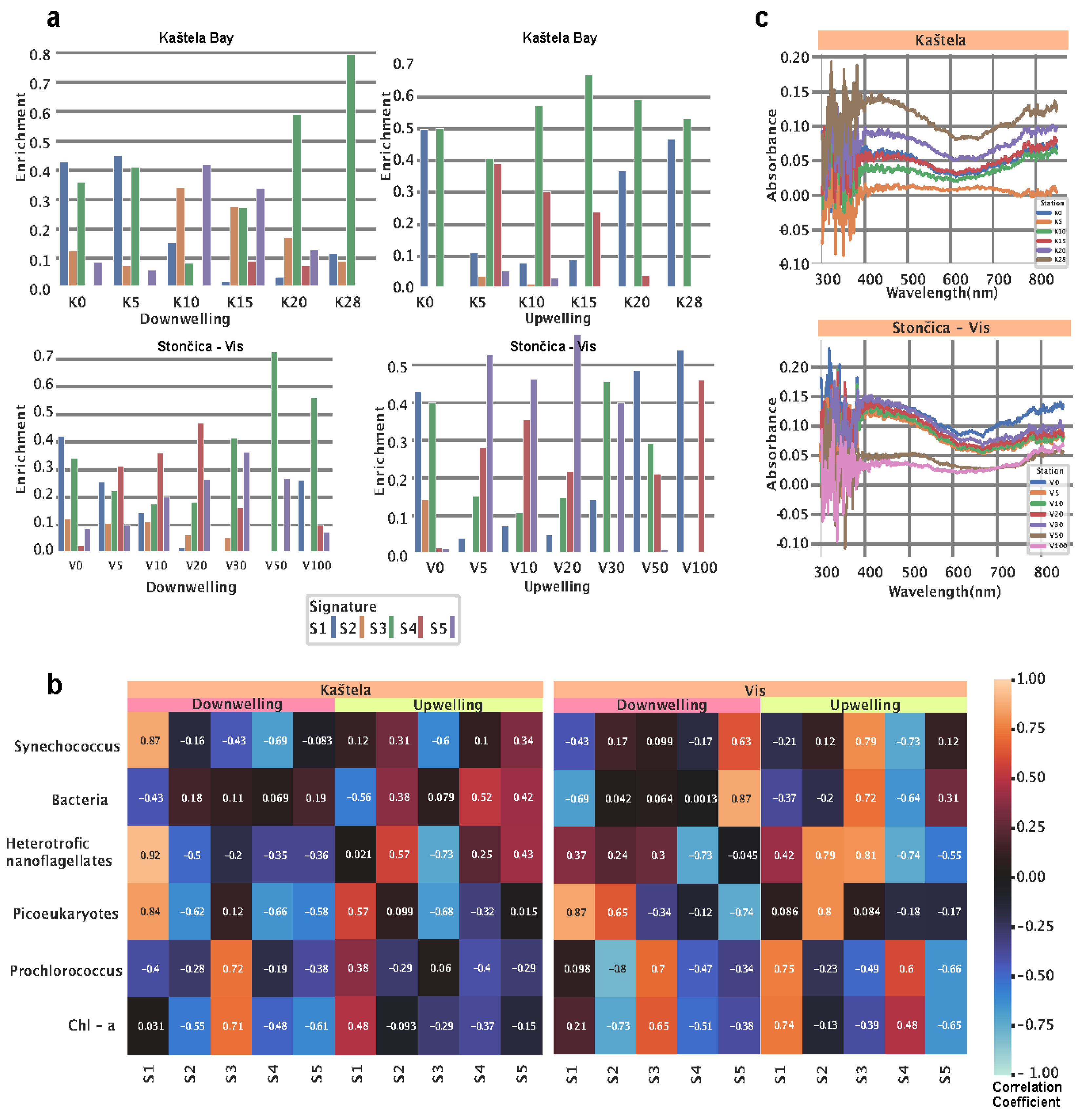
Figure 3.
Phytoplankton significance at two study locations. (a) Phytoplankton abundance at Kaštela - Bay and (b) Stončica - Vis study sites. Heatmaps (c,d) showing correlation between different phytoplankton taxa and extracted spectral signatures at (c) Kaštela - Bay site and (d) Stončica - Vis study sites. Correlations of phytoplankton taxa with Chlorophyll a (e) and particulate primary productivity (f).
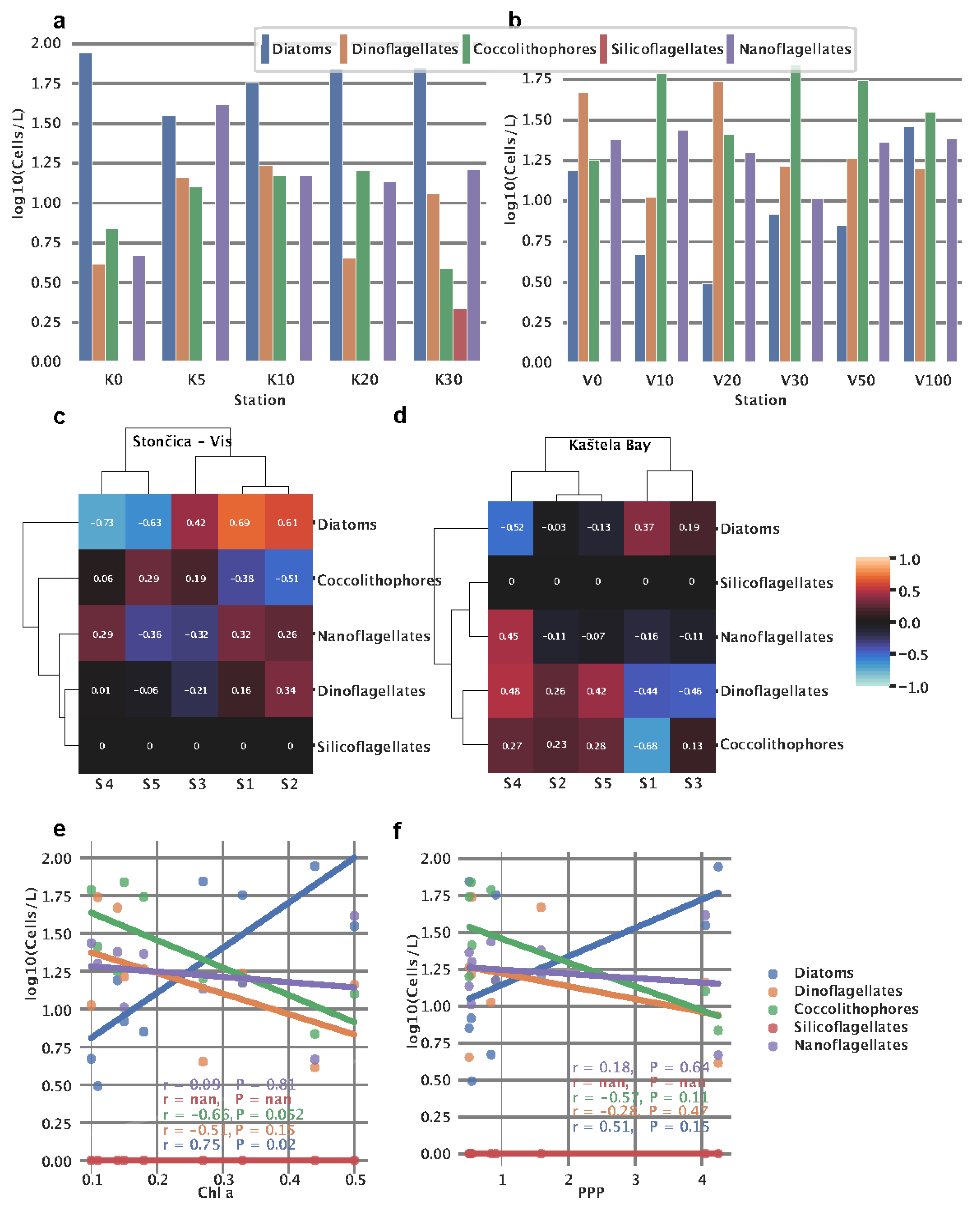
Figure 4.
Linear regression models for prediction of phytoplankton and cyanobacteria abundance. (a) %HNA bacteria, (b) bacteria, (c) heterotrophic nanoflagellates, (d) picoeukaryotes, (e) Prochlorococcus, and (f) Synechococcus.
Figure 4.
Linear regression models for prediction of phytoplankton and cyanobacteria abundance. (a) %HNA bacteria, (b) bacteria, (c) heterotrophic nanoflagellates, (d) picoeukaryotes, (e) Prochlorococcus, and (f) Synechococcus.
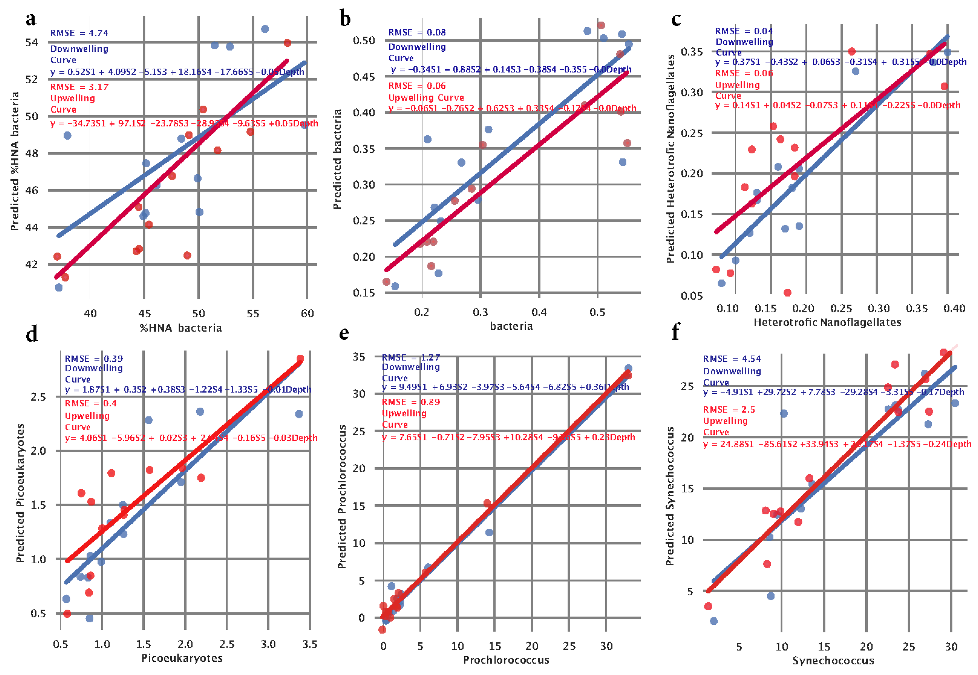

Table 1.
Summary of signature characteristics.
| Signature | Spectrum Assoc. | Depth assoc. (Training data) | Microbial Assoc. Kaštela | Microbial Assoc. Stončica Vis |
|---|---|---|---|---|
| S1 | Two peaks at 364 nm and 583 nm | UW: Positive | UW: PE(positive), PCO(positive), BAC (negative) |
UW: SNCO (negative), HNAN (positive), BAC (negative), PCO (positive) |
| DW: Minimal enrichment, around 40m | DW: SNCO (positive), HNAN(positive), PE(positive), BAC (negative), PCO (negative) |
DW: SNCO(negative),HNAN ( positive), PE(positive), BAC (negative) |
||
| S2 | High-intensity broad peak at 503 nm | UW: Minimal enrichment | UW: HNAN (positive), BAC(positive) |
UW: HNAN (positive) PE (positive) |
| DW: Negative convex | DW: PCO(negative), PE(negative), HNAN (negative), |
DW: PE(positive), PCO (negative) |
||
| S3 | Small peak at 493 nm | UW: Enriched at all depths (0-100m), mostly around 90m | UW: HNAN (negative), PE(negative), SNCO(negative) |
UW: SNCO (positive), BAC(positive), HNAN (positive), PCO(negative) |
| DW: Positive, mainly between 0-40m | DW: SNCO (negative), PCO (positive) |
DW: PCO (positive), PE (negative) |
||
| S4 | Low-Intensity, almost uniform at 353-573 nm | UW: Positive, mostly around 80m | UW: BAC(positive) |
UW: SNCO (negative), HNAN (negative),BAC(negative), PCO(positive) |
| DW: Highly enriched in 0-20m, minimal in depth > 20m | DW: SNCO (negative), HNAN (negative), PE(negative) |
DW: HNAN (negative), PCO(negative) |
||
| S5 | Low-intensity, covering broad spectrum 353-493 nm |
UW: Negative, mostly around 80m | UW: SNCO (positive), HNAN (positive), BAC(positive), |
UW: HNAN (negative), PCO(negative) |
| DW: Enriched at all depths (0-100m) | DW: HNAN (negative), PE(negative), PCO(negative) |
DW: PE(negative), PCO(negative), BAC(positive), SNCO (positive) |
Disclaimer/Publisher’s Note: The statements, opinions and data contained in all publications are solely those of the individual author(s) and contributor(s) and not of MDPI and/or the editor(s). MDPI and/or the editor(s) disclaim responsibility for any injury to people or property resulting from any ideas, methods, instructions or products referred to in the content. |
© 2024 by the authors. Licensee MDPI, Basel, Switzerland. This article is an open access article distributed under the terms and conditions of the Creative Commons Attribution (CC BY) license (http://creativecommons.org/licenses/by/4.0/).
Copyright: This open access article is published under a Creative Commons CC BY 4.0 license, which permit the free download, distribution, and reuse, provided that the author and preprint are cited in any reuse.


