
Submitted:
02 October 2025
Posted:
06 October 2025
You are already at the latest version
Abstract
Phytoplankton are fundamental to sustaining marine ecosystems and significantly in-fluence the global carbon cycle. However, to indetify their types accurately from sat-ellite imagery remains a challenge. This study presents machine learning approaches for classifying phytoplankton types, including coccolithophores, diatoms, and dino-flagellates, using Second-generation Global Imager (SGLI) imagery aboard the GCOM-C satellite. Several algorithms were evaluated, with Random Forest (RF) and Gradient Tree Boosting (GTB) achieving the highest classification performance. To assess model transferability, the developed machine learning models were applied in another sub-region and on a different date of acquisition. The validation confirmed the ability of the model to generalize across sub-region and temporal variations in SGLI imagery. As a result, the potential of combined machine learning and SGLI im-agery can improve phytoplankton detection, enabling large-scale monitoring at both regional and global levels. This paper highlights the importance of combining artifi-cial intelligence with satellite-derived ocean color data to improve the monitoring of marine ecosystems.
Keywords:
coccolithophore blooms
; diatom blooms
; dinoflagellate blooms
; machine learning
; random forest
; gradient tree boostig
; phytoplankton classification
; GCOM-C/SGLI
∙ Machine learning approaches were developed to classify
phytoplankton types, including coccolithophores, diatoms, and dinoflagellates,
using GCOM-C/SGLI satellite imagery.
∙ Random Forest (RF) and Gradient Tree Boosting (GTB) models
outperformed other tested algorithms, achieving high accuracy of classification
results.
∙ The developed machine learning models enable scalable monitoring
of phytoplankton blooms, supporting both regional and global ocean observation.
∙ Combined remote sensing with artificial intelligence can be used
as an alternative approach to monitor the marine ecosystem.
1. Introduction
Phytoplankton, key primary producers in the ocean, generate about 50% of global net primary production and thereby shape nutrient cycling, carbon dynamics, and climate regulation [1,2,3]. Coccolithophores, diatoms, and dinoflagellates are important phytoplankton functional groups, each with distinct ecological and biogeochemical roles [4,5].
Coccolithophores are unicellular eukaryotic phytoplankton that contribute significantly to the global carbon cycle through particulate inorganic carbon (PIC) production and calcification. Coccolithophores produce calcium carbonate (CaCO₃) plates (coccoliths) that regulate seawater optics and sustain the oceanic carbonate pump via calcification flux [6,7,8]. During blooms, detached coccoliths in suspension intensify backscattering and reflectance at times forming striking turquoise patches visible in satellite images [9,10]. These features complicate discrimination from non-calcifying taxa and suspended particulates [4,11]. Diatoms, by contrast, build siliceous frustules and dominate in high-nutrient, upwelling, or high-latitude regimes; they are among the most efficient drivers of organic carbon export (the biological pump) in many ocean regions [12,13,14]. Dinoflagellates are prominent drivers of harmful algal blooms (HABs) that threaten marine resources and ecosystem stability with trophic flexibility spanning autotrophy, heterotrophy, and mixotrophy [15,16,17]. Due to this diversity in physiological and optical traits, distinguishing these groups remotely is crucial for understanding ecosystem dynamics and carbon cycling.
Satellite ocean color remote sensing has been widely used to monitor phytoplankton distributions since the 1990s, via sensors such as SeaWiFS, MODIS, MERIS, and OLCI [18,19,20]. These platforms measure water-leaving reflectance, which is related to inherent optical properties (absorption and scattering) of water constituents. However, reliably discriminating phytoplankton functional types (PFTs) via conventional empirical or semi-analytical algorithms remains elusive. Coccolithophore optical signals often overlap with those from non-alkalinity variance and suspended sediments; traditional band-ratio or threshold-based indices yield ambiguous results in optically complex waters, leading to misclassification [4,21]. On the other hand, diatoms and dinoflagellates share overlapping pigment absorption features and scattering characteristics with other taxa, further confounding discrimination [22]. In coastal or turbid waters, high CDOM or suspended particulate load further degrades classification performance [23,24,25].
To address these limitations, machine learning (ML) has emerged as a promising path forward. Machine learning (ML) methods can be used to capture complex nonlinear relationships between spectral signatures and phytoplankton groups, which offers high performance on high-dimensional and noisy datasets [26,27]. Recent reviews highlight the growing integration of ML in ocean color retrieval, classification, and fusion tasks [28,29,30,31].
The GCOM-C (Shikisai) satellite mission, operated by JAXA, carries the Second-generation Global Imager (SGLI) sensor, offering 19 spectral bands across visible to shortwave infrared wavelengths and spatial resolutions from 250 m to 1000 m [32,33,34]. To maximize the potential of SGLI, a shift from conventional thresholds to a data-driven classification framework is required.
This study aims to develop a machine learning model to identify and classify coccolithophores, diatoms, and dinoflagellates using GCOM-C/SGLI imagery. Several machine learning algorithms will be evaluated and compared with particular emphasis on ensemble classifiers that have demonstrated high predictive performance. This study will also assess the developed machine learning models for another sub-region and on a different date of acquisition. The aim is to demonstrate the ability of the models to generalize across sub-regions and temporal variations in SGLI imagery. The implications of these findings are for operational monitoring of marine ecosystems.
2. Materials and Methods
2.1. Site Selection and Rationale
To demonstrate the reliability of the proposed method and ensure broader applicability, SGLI data from various study sub-regions in global areas were utilised in this study, as illustrated in Figure 1. Several existing studies have identified or confirmed the presence of optical water and phytoplankton types in different sub-regions, as described in Table 1, which were used to verify the presence of phytoplankton in these areas. This is to assist in creating datasets for a machine learning model.
2.2. GCOM-C/SGLI Data Acquisition and Extraction
The GCOM-C/SGLI provides 19 spectral bands at spatial resolutions ranging from 250 m to 1,000 m, with a global revisit time of approximately two days. Its unique bands, such as 380 nm UV and shortwave infrared, enhance its capacity to resolve atmospheric and oceanic processes. Level-2 SGLI products underwent atmospheric correction using JAXA’s standard algorithms, followed by cloud masking, radiometric calibration, and sunglint removal. Atmospheric correction was conducted using standard SGLI algorithms, ensuring removal of aerosol and Rayleigh scattering. Cloud and glint pixels were masked. The reflectance spectra were normalised to minimise illumination differences.
This study used the SGLI Level-2 dataset with the latest Version 3 atmospheric correction that includes remote sensing reflectance (Rrs, sr−1) and Chl-a at a spatial resolution of 250 m [43]. The Second-generation Global Imager (SGLI) measures remote-sensing reflectance (Rrs) at seven discrete wavelengths (380, 412, 443, 490, 530, 565, and 670 nm) spanning the ultraviolet to visible spectral range. Chl is usually used to identify the presence of phytoplankton, but it cannot be used to determine the type of phytoplankton accurately. Therefore, both Rrs and Chl were used to identify the type of phytoplankton for machine learning datasets.
2.3. Machine Learning Approach to Pytoplankton Identification and Classification
Chlorophyll classification using GCOM-C/SGLI imagery and machine learning is presented in Figure 1. A crucial aspect in implementing machine learning is the construction of an appropriate dataset, as it enables the model to learn and distinguish the target classes effectively. In this study, we employed remote sensing reflectance (RRS) at discrete wavelengths (380, 412, 443, 490, 530, 565, and 670 nm), hereafter denoted as b1–b7. Chlorophyll concentration values were incorporated to guide class definition, while published phytoplankton data were additionally utilized to ensure the dataset accurately represented each category. The dataset was divided into two: a training dataset for the learning process of the machine (70%) and a testing dataset to test the reliability of the machine learning model (30%). We also used bathymetry data (NOAA ETOPO1) to enhance classification accuracy, particularly in distinguishing between classes such as turbid waters and coccolithophore-dominated waters. The final model can be used to identify and classify phytoplankton in other areas or other acquisition dates of the GCOM-C/SGLI imagery.
This study used several machine learning methods to identify and classify phytoplankton. We used Random Forest (RF), Classification, Regression Tree (CART), and Gradient Tree Boosting (GTB). Tree-based algorithms, particularly Random Forest (RF) and Gradient Tree Boosting (GTB), have repeatedly demonstrated superior performance in remote sensing applications compared to traditional statistical classifiers such as Maximum Likelihood or Support Vector Machines (SVMs). Tree-based ensemble methods such as Random Forest (RF) and Gradient Tree Boosting (GTB) have consistently demonstrated superior performance in remote sensing classification tasks. Unlike parametric classifiers, these methods do not rely on distributional assumptions of spectral features and are therefore more robust when applied to heterogeneous environments. RF is widely recognized for its robustness and computational efficiency, while GTB has shown even higher accuracies in distinguishing spectrally overlapping classes, such as turbid waters and coccolithophore blooms. Compared to traditional methods (e.g., Maximum Likelihood, SVM, or kNN), these algorithms not only provide improved accuracy but also enhanced generalization capacity, making them particularly suitable for complex ocean-color and phytoplankton classification problems.
The Random Forest (RF) algorithm was employed in this study as the primary machine learning method due to its robustness and suitability for both classification and regression tasks. RF is an ensemble learning technique that combines the predictions of multiple decision trees to improve generalization performance and reduce overfitting. This method is based on the principle of bootstrap aggregating, whereby multiple subsets of the training dataset are generated through random sampling with replacement. Each subset is used to train an individual decision tree, thereby introducing diversity among the base learners.
During the construction of each tree, a random subset of features is selected at every decision node rather than considering the entire feature set. This randomization ensures low correlation among trees and further enhances the ensemble’s predictive power. Each decision tree is grown to its maximum extent without pruning, which allows the trees to capture complex patterns in the data. For classification tasks, the final prediction is determined through majority voting across all trees. Mathematically, the Random Forest prediction for classification can be expressed as:
Where denotes the prediction of the decision tree and represents the total number of trees in the forest. Several hyperparameters govern the performance of the Random Forest model. The number of trees () influences the stability and accuracy of the predictions, while the maximum number of features considered at each split () controls the diversity among trees. Tree complexity is managed through parameters such as maximum depth () and the minimum number of samples per split or leaf, which serve as stopping criteria during tree construction.
The RF algorithm offers several advantages, including resilience to noisy data and outliers, the capacity to handle high-dimensional feature spaces, and the provision of internal estimates of feature importance, which enhance interpretability.
Classification and Regression Trees (CART) represent a non-parametric supervised machine learning approach that partitions input data into homogeneous subsets. The final model is structured as a binary tree in which terminal nodes correspond to predicted classes or continuous values. CART offers simplicity, interpretability, and direct feature selection, but its predictive accuracy is often constrained by high variance and sensitivity to noise, particularly in heterogeneous remote sensing environments.
On the other hand, Gradient Tree Boosting (GTB) is an advanced ensemble learning approach that constructs predictive models by sequentially combining multiple decision trees, where each tree is trained to correct the residual errors of the preceding ones. GTB has become a widely adopted technique due to its ability to handle high-dimensional, heterogeneous, and often noisy spectral and spatial features. Therefore, this classifier is suitable to address complex ocean-color and phytoplankton classification issues.
2.4. Assessment of the Results
To ensure the robustness and generalizability of the model, the performance of the classification model was assessed using a confusion matrix, which provides a comprehensive comparison between predicted and actual class labels. The matrix summarizes classification outcomes in terms of correctly and incorrectly classified samples, structured as true positives, true negatives, false positives, and false negatives. From this matrix, several evaluation metrics were derived, namely Producer’s Accuracy, User’s Accuracy, Overall Accuracy, and the Kappa Coefficient, which together provide a rigorous assessment of classification reliability.
Producer’s Accuracy (PA) represents the probability that a reference sample of a given class is correctly classified. It is calculated as the ratio of correctly classified samples in a particular class to the total number of reference samples for that class. PA is analogous to recall or sensitivity, and it reflects how well the classifier can recognize members of a given class:
User’s Accuracy (UA) measures the probability that a sample classified into a given class actually belongs to that class. It is calculated as the ratio of correctly classified samples in a class to the total number of samples assigned to that class. UA is equivalent to precision, and it indicates the reliability of the classification from the user’s perspective:
Overall Accuracy (OA) provides a general measure of classification performance by dividing the total number of correctly classified samples by the total number of samples in the dataset:
Where is the total number of samples across all classes. While OA is widely used, it may not fully capture classification reliability in the presence of class imbalance. To address this limitation, the was calculated. Kappa measures the agreement between the classification results and the reference data, adjusted for the agreement that could occur by chance. It is expressed as:
Whereis the hypothetical probability of chance agreement, calculated from the row and column totals of the confusion matrix.
3. Results
The identification and classification of phytoplankton using GCOM-C/SGLI imagery are divided by phytoplankton types, i.e., coccolithophores, diatoms and dinoflagellates. Each type of phytoplankton in this study will be identified using several machine learning methods in this section, and will be analysed to find the best machine learning model. We divided the datasets into two parts: 70% for the training datasets and 30% for the testing datasets.
We conducted some scenarios with different inputs for these ML models and tested them to find the best scenario. The scenarios are utilising: (1) seven bands of SGLI data, (2) six bands of SGLI data excluded Rrs380, and (3) seven bands of SGLI data and chlorophyll data (Chl).
3.1. Coccolithophore Blooms Identification and Classification
Three classifiers, i.e., Random Forest (RF), Classification and Regression Tree (CART), and Gradient Boosted Trees (GBT), were tested to identify and classify coccolithophore blooms in Sagami Bay, Japan. The following are the results of coccolithophore blooms identification and classification using various scenarios with three different ML classifiers.
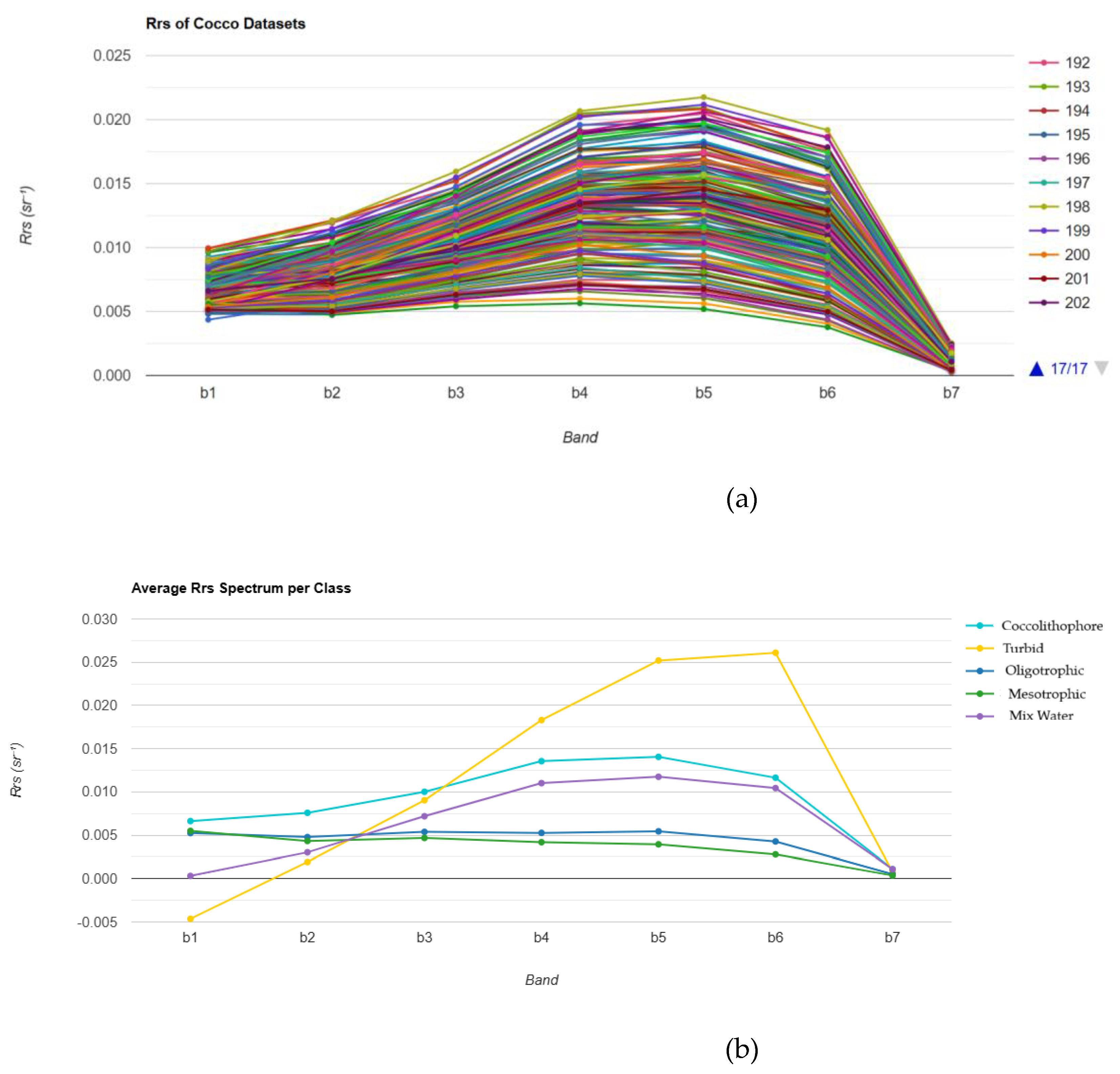
Figures 2(a) and 1(b) show the Rrs value of each class provided from the datasets and the average Rrs values for each class, with Rrs plotted against different spectral bands (B1 to B7), respectively. The turbid water demonstrates the strongest reflectance in almost all bands. It reaches a peak around B5 and Bb6, which indicates a high concentration of suspended particles that scatter light. The presence of coccolithophores can also be identified by their high reflectance in the visible band.
Figure 2.
(a) The Rrs values of coccolitophore datasets. (b) Average Rrs value for each class.
We can see the classification results visually in Figure 3, all classifiers classify each class accurately. All classifiers obtained high accuracy results, with their accuracy varying across scenarios (Table 2). In the seven bands scenario, the GBT classifier achieved the best result, with an overall accuracy of 98.4% (Kappa = 0.975), followed by the RF, which achieved 97.6% accuracy (Kappa = 0.962). CART also produced competitive results (96.7%, Kappa = 0.950), although its classification threshold was less precise.
The results showed that excluding band 1 (Rrs380) made a significant decrease in accuracy, as tested in RF (Accuracy = 93.9%, Kappa = 0.911), highlighting the importance of the Rrs380 for detecting coccolithophores. This finding is consistent with previous research highlighting how coccolithophore blooms, which are rich in calcite plates, exhibit strong backscatter signals at shorter wavelengths.
To validate the proposed method, we tested the ML model obtained in the previous process in another sub-region in the south of Plymouth City in the English Channel area. We can see visually in Figure 4 that the classification result shows high accuracy. However, there is an oddity in the detection of coccolithophores in deep-sea areas due to the detected turbidity, as turbidity is usually caused by suspended particles such as mud, clay, and organic matter in the water and is found in shallow waters. This anomaly was checked with chlorophyll data in GCOM-C/SGLI and showed that the chlorophyll concentration in the area was very high. This indicates that the area is a coccolithophore because the surrounding area was also detected by the phytoplankton. To address this issue, the proposed method used bathymetry data from ETOPO1 to separate the turbid and coccolithophore classes to achieve more accurate classification results. It shows promising results because the deep-sea area that was originally classified as turbid has been reclassified as the correct class, which is what it should be.
3.2. Diatom Blooms Identification and Classification
The following are the results of diatom blooms identification and classification using various scenarios with three different ML classifiers. The Figure 5 presents the average remote sensing reflectance (Rrs) spectra across different air classes—Diatom, Low Diatom, Turbid, and Clear—plotted against b1 to b7 the spectral bands. Across all classes, Rrs values are lowest at b1 (shorter wavelengths), gradually increasing towards the b2 to b4 visible spectrum, before decreasing again at longer wavelengths (b6 to b7). Diatom and Low-Diatom waters show enhanced reflectance in b3 to b6 due to phytoplankton pigment absorption, dominated by chlorophyll-a near b4 to b5. Turbid waters show the highest reflectance across all bands, which reflects the strong backscattering caused by suspended particles that is characteristic of turbid conditions.
Diatom classification using GCOM-C SGLI images and machine learning algorithms showed high performance across all tested scenarios (Table 3, Figure 6). The RF and GTB model with seven spectral bands achieved the highest accuracy at 0.978 (Kappa = 0.969). The RF model trained with six bands produced slightly lower but still robust results (Overall Accuracy = 0.964, Kappa = 0.950). The CART algorithm using seven bands performed comparably with Overall Accuracy at 0.966 (Kappa = 0.953).
These findings indicate that the inclusion of all seven spectral bands improves the accuracy of the results, while the removal of even one band results in a measurable decrease in performance. Among the classifiers, the RF and GTB have outperformed the single tree approach (CART) in handling the spectral variability of diatoms. Classification results show that diatom identification using GCOM-C SGLI is feasible with high reliability, particularly when machine learning methods are employed and complete spectral information is used.
We validated the developed RF model with seven bands of SGLI data from a different acquisition date to assess its reliability. The classification result in Figure 7 shows that it was successful in identifying diatoms, aligning with the original training dataset. While minor discrepancies were found, the validation confirmed the ability of the model to generalize across temporal variations in SGLI imagery.
3.3. Dinoflagellate Blooms Identification and Classification
The following are the results of dinoflagellate blooms identification and classification using various scenarios with three different ML classifiers. Figure 8 shows the average Rrs spectra across seven spectral bands for six distinct water classes, including harmful algal bloom (HAB) cases (Karenia and Karenia-low), mixed phytoplankton assemblages (Mix-low and Mix-high), turbid waters, and clear waters. The Karenia and Karenia-low classes have low reflectance across all bands, particularly in the b1 to b4 visible range. This spectral depression reflects the high chlorophyll-a and accessory pigment concentrations typical of dense Karenia blooms, which dominate light absorption and suppress water-leaving radiance.
The RF, CART, and GTB classifiers with seven bands generated bloom detections that closely matched the SGLI baseline, with minimal misclassification and clear delineation of bloom boundaries. Dinoflagellate blooms were identified and classified using GCOM-C SGLI data combined with RF, CHART, and GTB (Figure 9). Overall accuracies and Kappa coefficients for the tested scenarios are presented in Table 3. The RF and CART classifiers using seven spectral bands produced the highest accuracies, with an overall accuracy of 0.988 and corresponding Kappa coefficients of 0.982. In contrast, reducing the RF input to six bands resulted in a decline in performance, with an overall accuracy of 0.922 and a Kappa coefficient of 0.888. GTB with seven bands also demonstrated strong performance but was slightly less accurate, yielding an overall accuracy of 0.976 and a Kappa coefficient of 0.963.

Table 4.
Accuracies of the results.
| Scenario | Overall Accuracy | Kappa Coefficient |
|---|---|---|
| RF with seven bands | 0.9879518072289156 | 0.9816534040671971 |
| RF with six bands | 0.9215686274509803 | 0.8879890185312285 |
| CART with seven bands | 0.9879518072289156 | 0.9815062388591798 |
| GTB with seven bands | 0.9759036144578314 | 0.9631602308033732 |
4. Discussion
Our results confirm the effectiveness of ML approaches for coccolithophore bloom classification. RF and GTB have superior performance, reflecting their ability to capture nonlinearities and interactions across multiple spectral bands. Interestingly, CART underperformed compared to expectations, possibly due to the relatively limited size of training data, as it is a single decision tree model.
To assess model transferability, the classifiers were applied in another sub-region and on a different date of acquisition. The RF model for coccolithophore classification was tested in another sub-region, south of Plymouth City, in the English Channel area, under two conditions: with and without bathymetric data (Figure 3). Results showed that including bathymetric information improved classification accuracy. This suggests that coupling remote sensing reflectance with geophysical context enhances the robustness of monitoring open-ocean coccolithophore blooms.
In the diatom classification results, the reduction from seven to six spectral bands in the RF model led to a decline in both overall accuracy (−1.3%) and Kappa (−1.9%), demonstrating the sensitivity of diatom classification to the availability of complete spectral information. Thus, preserving the complete SGLI spectral set is crucial for achieving high accuracy. The RF and GTB approaches outperformed the single-tree CART algorithm. This superiority reflects the ability of the methods to reduce variance and avoid overfitting, which is particularly relevant in remote sensing classification, where spectral responses can be confounded by water constituents such as colored dissolved organic matter and suspended sediments. The performance of RF and GTB suggests that both approaches are robust to diatom variability. However, RF may offer operational advantages due to its lower computational cost and interpretability. The validation result demonstrated that the RF classifier performs robustly across temporal variability, suggesting that the spectral signatures of diatoms are sufficiently stable to allow consistent identification in different seasonal or environmental contexts.
The results of dinoflagellate classification highlight the strong potential of machine learning classifiers, particularly RF and CART, for detecting and classifying dinoflagellate blooms from SGLI data. These results demonstrate the value of GCOM-C SGLI data for operational monitoring of harmful algal blooms (HABs). The high classification accuracy achieved indicates that SGLI provides sufficient spectral coverage and resolution for distinguishing dinoflagellates from other optical water types, which is essential for early warning systems and ecological assessments.
5. Conclusions
This study demonstrated the effectiveness of machine learning models, particularly Random Forest and Gradient Tree Boosting, in classifying phytoplankton, including coccolithophores, diatoms, and dinoflagellates, using GCOM-C/SGLI imagery. These findings could inform an alternative approach to operational monitoring of phytoplankton on regional and global scales.
Despite encouraging results, some limitations warrant consideration. First, classification accuracies may vary under conditions of optically complex waters, where non-algal particles and dissolved organic matter confound spectral signals. Validation with in situ datasets across diverse aquatic environments is needed to confirm model generalizability. Second, while GCOM-C SGLI provides sufficient spectral coverage for diatom detection, hyperspectral sensors such as PACE OCI could further improve discrimination of phytoplankton functional types. Future work should also explore temporal dynamics, including seasonal blooms, to assess the potential of SGLI for long-term ecosystem monitoring.
Author Contributions
“Conceptualization, D.S.C. and E.S.; methodology, D.S.C. and E.S.; software, D.S.C; validation, D.S.C. and E.S.; formal analysis, D.S.C. and E.S.; investigation, D.S.C. and E.S.; resources, D.S.C. and E.S.; data curation, D.S.C. and E.S.; writing—original draft preparation, D.S.C. and E.S.; writing—review and editing, D.S.C. and E.S.; visualization, D.S.C. All authors have read and agreed to the published version of the manuscript.
Funding
This research was supported by the Japan Aerospace Exploration Agency–3rd Research Announcement on the Earth Observations [JAXA–3th EORA, contract: 24RT000233], the Asia-Pacific Network for Global Change Research [APN, CRRP2024-05MY-Siswanto], and Grants-in-Aid for Scientific Research [KAKENHI JP21H05317] from the Ministry of Education, Culture, Sports, Science, and Technology-Japan (MEXT).
Acknowledgments
The authors would like to extend thanks to Research Center for Geoinformatics, Research Organization for Electronics and Informatics, National Research and Innovation Agency of Indonesia (BRIN.
Conflicts of Interest
The authors declare no conflicts of interest.
References
- T. J. Ryan-Keogh, S. J. Thomalla, N. Chang, and T. Moalusi, “A new global oceanic multi-model net primary productivity data product,” Earth Syst Sci Data, vol. 15, no. 11, pp. 4829– 4848, 2023. [CrossRef]
- G. M. Silsbe, J. Fox, T. K. Westberry, and K. H. Halsey, “Global declines in net primary production in the ocean color era,” Nat Commun, vol. 16, no. 1, p. 5821, 2025. [CrossRef]
- E. Litchman, P. E. Litchman, P. de Tezanos Pinto, K. F. Edwards, C. A. Klausmeier, C. T. Kremer, and M. K. Thomas, “Global biogeochemical impacts of phytoplankton: a trait-based perspective,” Journal of Ecology, vol. 103, no. 6, pp. 1384–1396, Nov. 2015. [Google Scholar] [CrossRef]
- T. Moore, M. T. Moore, M. Dowell, and B. Franz, “Detection of coccolithophore blooms in ocean color satellite imagery: A generalized approach for use with multiple sensors,” Remote Sensing of Environment - REMOTE SENS ENVIRON, vol. 117, Dec. 2011. [Google Scholar] [CrossRef]
- S. I. Anderson, A. D. Barton, S. Clayton, S. Dutkiewicz, and T. A. Rynearson, “Marine phytoplankton functional types exhibit diverse responses to thermal change,” Nat Commun, vol. 12, no. 1, p. 6413, 2021. [CrossRef]
- R. El Hourany, J. R. El Hourany, J. Pierella Karlusich, L. Zinger, H. Loisel, M. Levy, and C. Bowler, “Linking satellites to genes with machine learning to estimate phytoplankton community structure from space,” Ocean Science, vol. 20, no. 1, pp. 2024. [Google Scholar] [CrossRef]
- W. M. Balch, B. C. W. M. Balch, B. C. Bowler, D. T. Drapeau, L. C. Lubelczyk, and E. Lyczkowski, “Vertical Distributions of Coccolithophores, PIC, POC, Biogenic Silica, and Chlorophyll a Throughout the Global Ocean,” Global Biogeochem Cycles, vol. 32, no. 1, pp. 2–17, Jan. 2018. [Google Scholar] [CrossRef]
- W. M. Balch and C. Mitchell, “Remote sensing algorithms for particulate inorganic carbon (PIC) and the global cycle of PIC,” Earth Sci Rev, vol. 239, p. 10 4363, 2023. [CrossRef]
- A. Grubb, C. A. Grubb, C. Johns, M. Hayden, A. Subhas, K. Thamatrakoln, and K. Bidle, “Calcification increases carbon supply, photosynthesis, and growth in a globally distributed coccolithophore,” Limnol Oceanogr, vol. 69, pp. 2152–2166, Aug. 2024. [Google Scholar] [CrossRef]
- “Optical Modeling of Spectral Backscattering and Remote Sensing Reflectance From Emiliania huxleyi Blooms”.
- I. Cetinić et al., “Phytoplankton composition from sPACE: Requirements, opportunities, and challenges,” Remote Sens Environ, vol. 302, p. 11 3964, 2024. [CrossRef]
- J. R. Williams et al., “Inefficient transfer of diatoms through the subpolar Southern Ocean twilight zone,” Nat Geosci, vol. 18, no. 1, pp. 2025; 77. [CrossRef]
- F. Abrantes et al., “Diatoms Si uptake capacity drives carbon export in coastal upwelling systems,” Biogeosciences, vol. 13, no. 14, pp. 4099– 4109, 2016. [CrossRef]
- “Sinking Diatom Assemblages as a Key Driver for Deep Carbon and Silicon Export in the Scotia Sea”.
- M. E. Larsson et al., “Mucospheres produced by a mixotrophic protist impact ocean carbon cycling,” Nat Commun, vol. 13, no. 1, p. 1301, 2022. [CrossRef]
- K. Möller et al., “Effects of bottom-up factors on growth and toxin content of a harmful algae bloom dinoflagellate,” Limnol Oceanogr, vol. 69, no. 6, pp. 1335–1349, Jun. 2024. [CrossRef]
- M. R. Mulholland, R. Morse, T. Egerton, P. W. Bernhardt, and K. C. Filippino, “Blooms of Dinoflagellate Mixotrophs in a Lower Chesapeake Bay Tributary: Carbon and Nitrogen Uptake over Diurnal, Seasonal, and Interannual Timescales,” Estuaries and Coasts, vol. 41, no. 6, pp. 1744– 1765, 2018. [CrossRef]
- “Satellite Ocean Colour-Current Status and Future Perspective”.
- D. Odermatt, A. D. Odermatt, A. Gitelson, V. E. Brando, and M. Schaepman, “Review of constituent retrieval in optically deep and complex waters from satellite imagery,” Remote Sens Environ, vol. 118, pp. 2012. [Google Scholar] [CrossRef]
- D. Blondeau-Patissier, J. F. R. D. Blondeau-Patissier, J. F. R. Gower, A. G. Dekker, S. R. Phinn, and V. E. Brando, “A review of ocean color remote sensing methods and statistical techniques for the detection, mapping and analysis of phytoplankton blooms in coastal and open oceans,” Prog Oceanogr, vol. 123, pp. 2014. [Google Scholar] [CrossRef]
- W. M. Balch and C. Mitchell, “Remote sensing algorithms for particulate inorganic carbon (PIC) and the global cycle of PIC,” Apr. 01, 2023, Elsevier B.V. [CrossRef]
- Y. Zhang, F. Shen, H. Zhao, X. Sun, Q. Zhu, and M. Li, “Optical distinguishability of phytoplankton species and its implications for hyperspectral remote sensing discrimination potential,” J Sea Res, vol. 202, p. 10 2540, 2024. [CrossRef]
- A. Ansper-Toomsalu, M. Uusõue, K. Kangro, M. Hieronymi, and K. Alikas, “Suitability of different in-water algorithms for eutrophic and absorbing waters applied to Sentinel-2 MSI and Sentinel-3 OLCI data,” Frontiers in Remote Sensing, vol. Volume 5- 2024, 2024. [CrossRef]
- S. Bi and M. Hieronymi, “Holistic optical water type classification for ocean, coastal, and inland waters,” Limnol Oceanogr, vol. 69, no. 7, pp. 1547–1561, Jul. 2024. [CrossRef]
- Z. Wu et al., “A review of remote sensing-based water quality monitoring in turbid coastal waters,” Intelligent Marine Technology and Systems, vol. 3, no. 1, p. 2025; 24. [CrossRef]
- H. Bachimanchi et al., “Deep-learning-powered data analysis in plankton ecology,” Limnol Oceanogr Lett, vol. 9, no. 4, pp. 324–339, Aug. 2024. [CrossRef]
- Z. Li, W. Z. Li, W. Yang, B. Matsushita, and A. Kondoh, “Remote estimation of phytoplankton primary production in clear to turbid waters by integrating a semi-analytical model with a machine learning algorithm,” Remote Sens Environ, vol. 275, p. 113027, Jun. 2022. [Google Scholar] [CrossRef]
- “A Review of Machine Learning Applications”.
- “Using Machine Learning for Timely Estimates of Ocean Color Information From Hyperspectral Satellite Measurements in the Presence of Clouds”.
- “Deep-learning-based information mining from ocean remote-sensing imagery”.
- “An Artificial Neural Network Algorithm to Retrieve Chlorophyll a for Northwest European Shelf Seas from Top of Atmosphere Ocean Colour Reflectance”.
- “Long-Term Evaluation of GCOM-C-SGLI Reflectance and Water Quality Products”.
- T. Y. Nakajima et al., “Theoretical basis of the algorithms and early phase results of the GCOM-C (Shikisai) SGLI cloud products,” Prog Earth Planet Sci, vol. 6, no. 1, p. 2019; 52. [CrossRef]
- L. Zheng, Z. Lee, Y. Wang, X. Yu, W. Lai, and S. Shang, “Evaluation of near-blue UV remote sensing reflectance over the global ocean from SNPP VIIRS, PACE OCI, and GCOM-C SGLI,” Opt Express, vol. 33, no. 19, pp. 40465–4 0488, 2025. [Google Scholar] [CrossRef]
- C. K. Tan, J. C. K. Tan, J. Ishizaka, S. Matsumura, F. Md. Yusoff, and Mohd. I. Hj. Mohamed, “Seasonal variability of SeaWiFS chlorophyll a in the Malacca Straits in relation to Asian monsoon,” Cont Shelf Res, vol. 26, no. 2, pp. 2006. [Google Scholar] [CrossRef]
- H. Yamaguchi, J. H. Yamaguchi, J. Ishizaka, E. Siswanto, Y. Baek Son, S. Yoo, and Y. Kiyomoto, “Seasonal and spring interannual variations in satellite-observed chlorophyll-a in the Yellow and East China Seas: New datasets with reduced interference from high concentration of resuspended sediment,” Cont Shelf Res, vol. 59, pp. 20 May; 9. [CrossRef]
- Y. Wang, D. Y. Wang, D. Liu, Y. Wang, Z. Gao, and J. K. Keesing, “Evaluation of standard and regional satellite chlorophyll-a algorithms for moderate-resolution imaging spectroradiometer (MODIS) in the Bohai and Yellow Seas, China: a comparison of chlorophyll-a magnitude and seasonality,” Int J Remote Sens, vol. 40, no. 13, pp. 4980–4995, Jul. 2019. [Google Scholar] [CrossRef]
- K. Furukawa, “Eutrophication in Tokyo Bay,” in Eutrophication and Oligotrophication in Japanese Estuaries: The present status and future tasks, T. Yanagi, Ed., Dordrecht: Springer Netherlands, 2015, pp. 5–37. [CrossRef]
- A. Kubo, Y. A. Kubo, Y. Yamashita, F. Hashihama, and J. Kanda, “The origin and characteristics of dissolved organic carbon in the highly urbanized coastal waters of Tokyo Bay,” J Oceanogr, vol. 79, no. 3, pp. 2023. [Google Scholar] [CrossRef]
- K. Yano, Y. K. Yano, Y. Takayama, S. Shimode, M. Toratani, H. Murakami, and V. S. Kuwahara, “Observation of a coccolithophore Gephyrocapsa oceanica bloom in the temperate coastal waters of Sagami Bay, Japan,” Plankton Benthos Res, vol. 19, no. 1, pp. 2024; 50. [Google Scholar] [CrossRef]
- “Distribution of Harmful Algae (Karenia spp.) in 21 Off Southeast Hokkaido”. 20 October.
- E. Siswanto, J. E. Siswanto, J. Luang-on, K. Ogata, H. Higa, and M. Toratani, “Observations of water optical properties during red tide outbreaks off southeast Hokkaido by GCOM-C/SGLI: implications for the development of red tide algorithms,” Remote Sensing Letters, vol. 15, no. 2, pp. 121–132, Feb. 2024. [Google Scholar] [CrossRef]
- H. Murakami, D. H. Murakami, D. Antoine, V. Vellucci, and R. Frouin, “System vicarious calibration of GCOM-C/SGLI visible and near-infrared channels,” J Oceanogr, vol. 78, no. 4, pp. 2022. [Google Scholar] [CrossRef]
Figure 1.
Flowchart of Chlorophyll Classification using GCOM-C/SGLI imagery and Machine Learning.
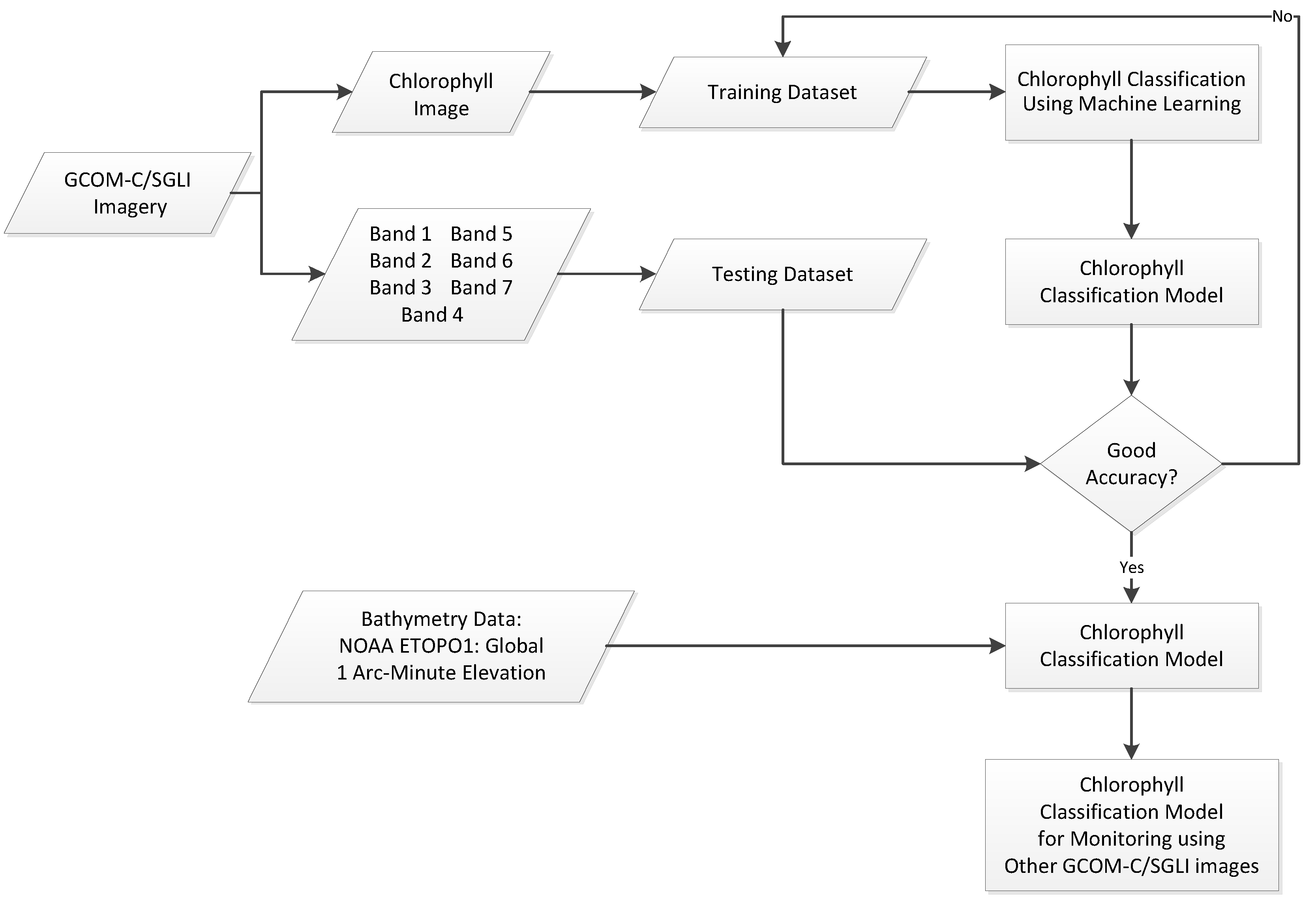
Figure 3.
Coccolithophore classification results for some scenarios. (a) SGLI data, (b) Classification results using RF with seven bands as the inputs, (c) Classification results using RF with six bands as the inputs, (d) Classification results using CART with seven bands as the inputs, and (e) Classification results using GTB with seven bands as the inputs.
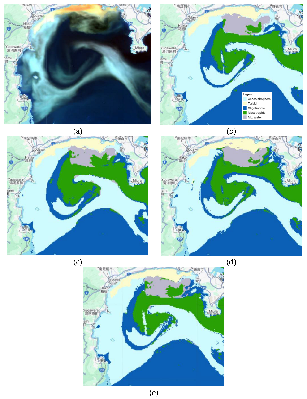
Figure 4.
Coccolithophore classification results for some scenarios in another sub-region in the south of Plymouth City in the English Channel area. (a) SGLI data, (b) Classification results using RF with seven bands as the inputs without bathymetry data, (c) Classification results using RF with seven bands as the inputs with bathymetry data.
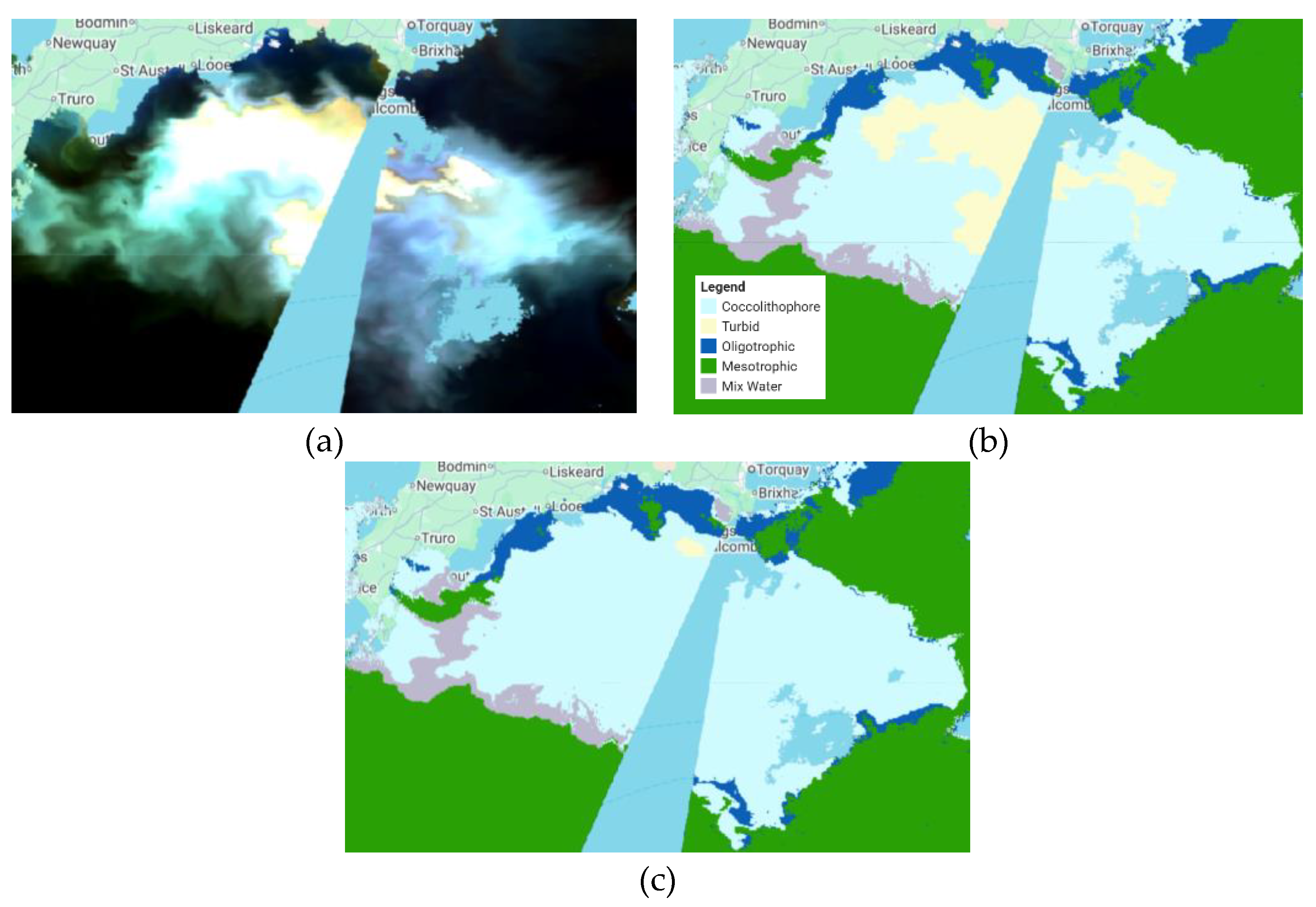
Figure 5.
(a) The Rrs values of diatom datasets. (b) Average Rrs value for each class.
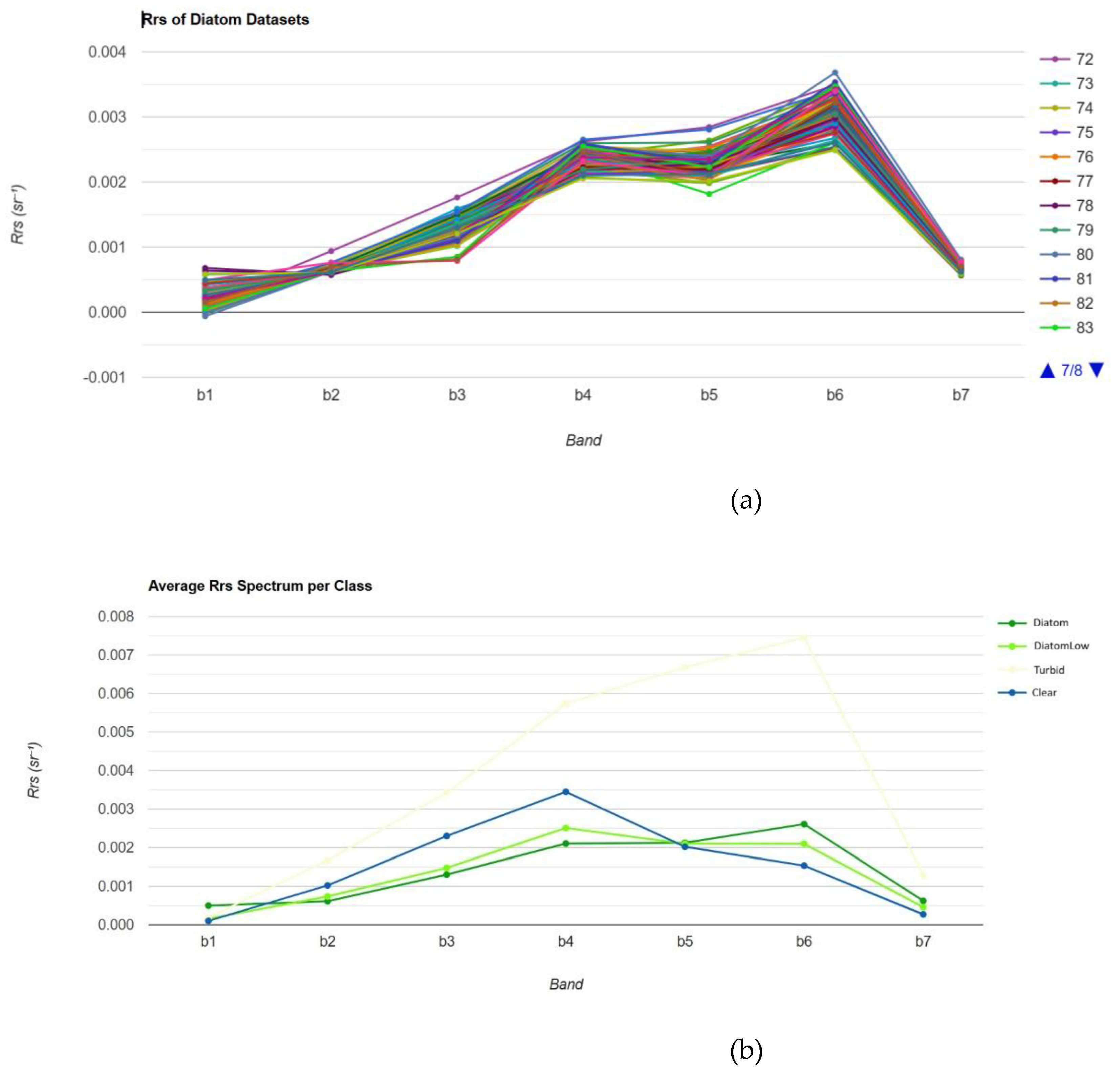
Figure 6.
Diatom classification results with some scenarios. (a) SGLI data, (b) Classification results using RF with seven bands as the inputs, (c) Classification results using RF with six bands as the inputs, (d) Classification results using CART with seven bands as the inputs, and (e) Classification results using GTB with seven bands as the inputs.
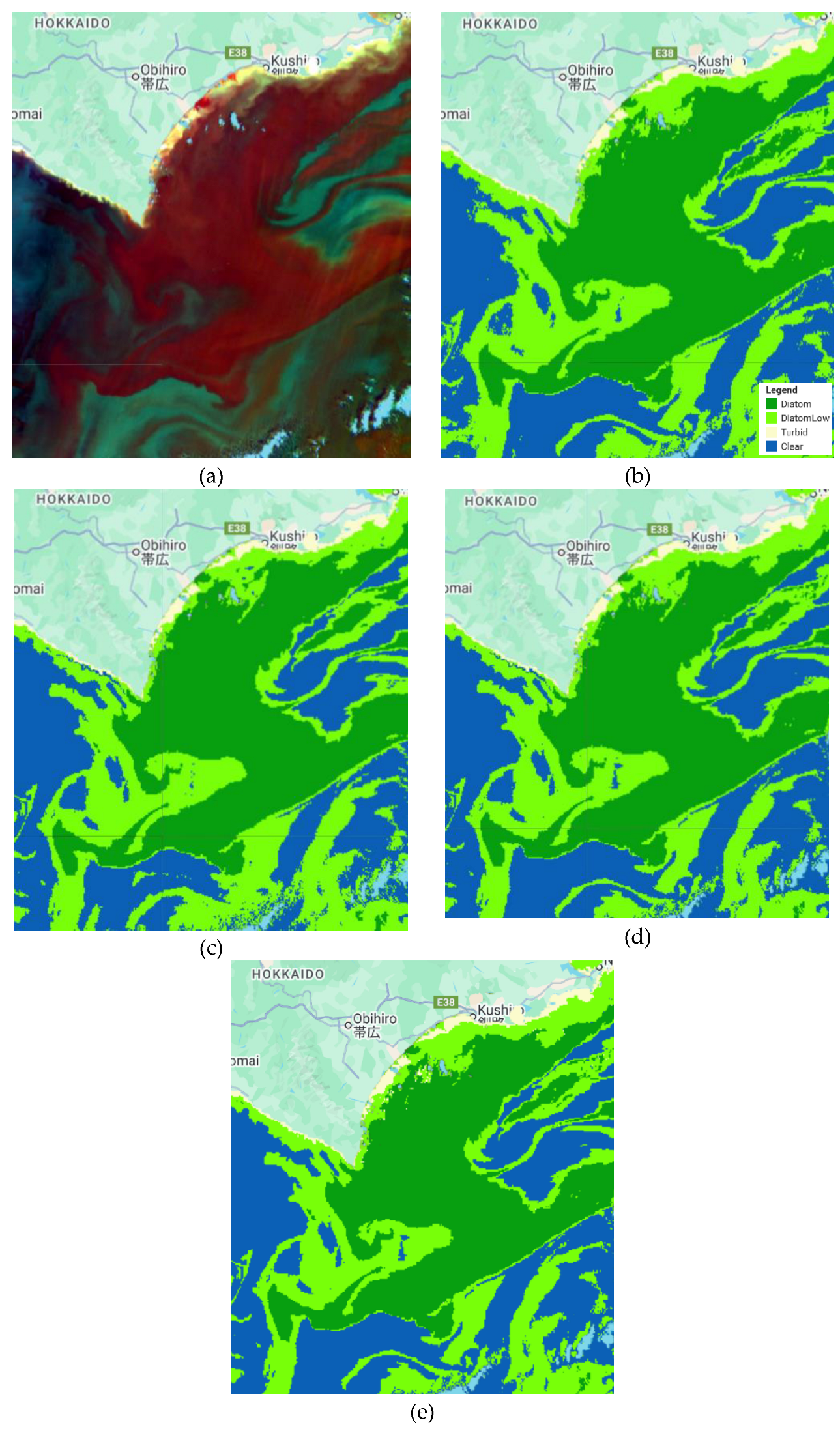
Figure 7.
Diatom classification results from a different acquisition date. (a) SGLI data, (b) Classification results using RF with seven bands as the inputs.
Figure 7.
Diatom classification results from a different acquisition date. (a) SGLI data, (b) Classification results using RF with seven bands as the inputs.
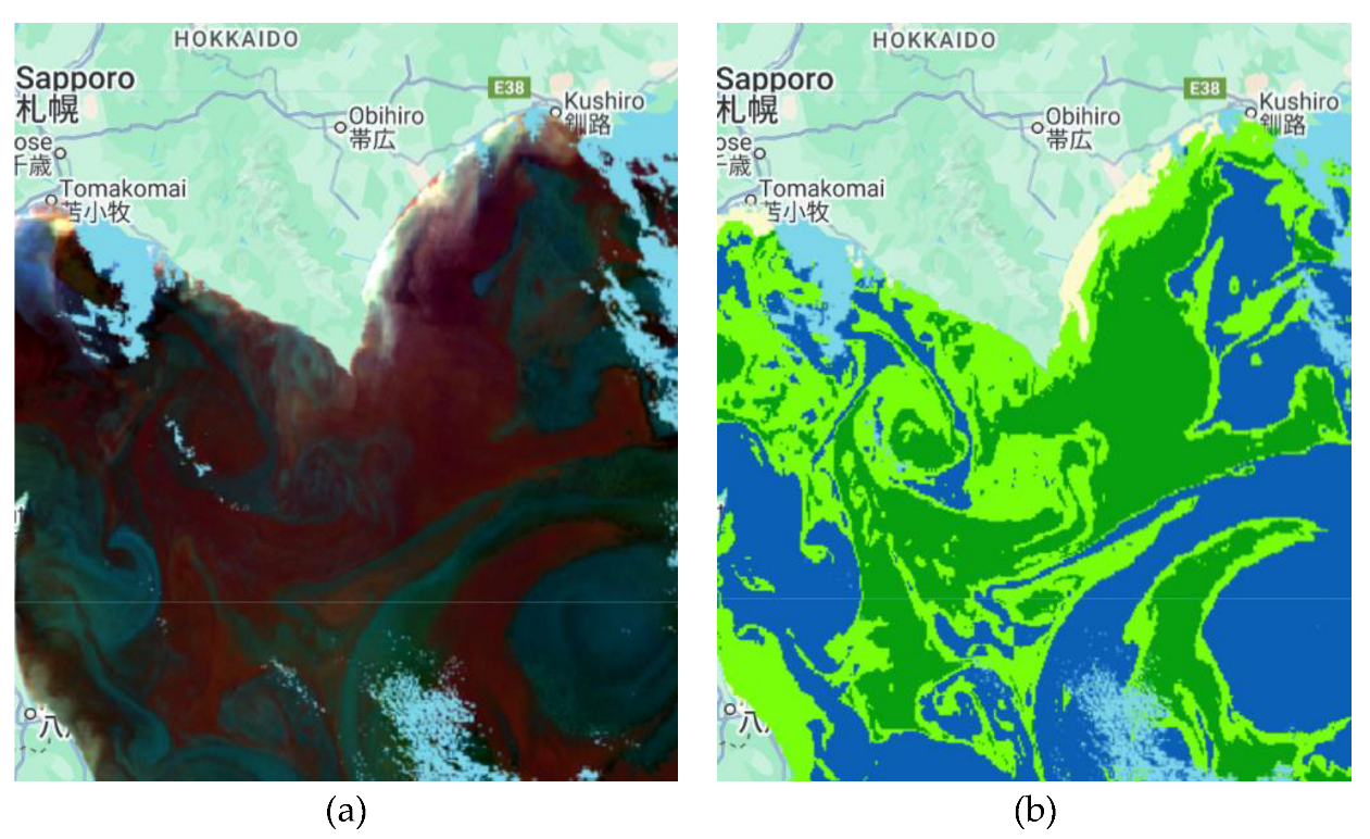
Figure 8.
(a) The Rrs values of dinoflagellate (Karenia) datasets. (b) Average Rrs value for each class.
Figure 8.
(a) The Rrs values of dinoflagellate (Karenia) datasets. (b) Average Rrs value for each class.
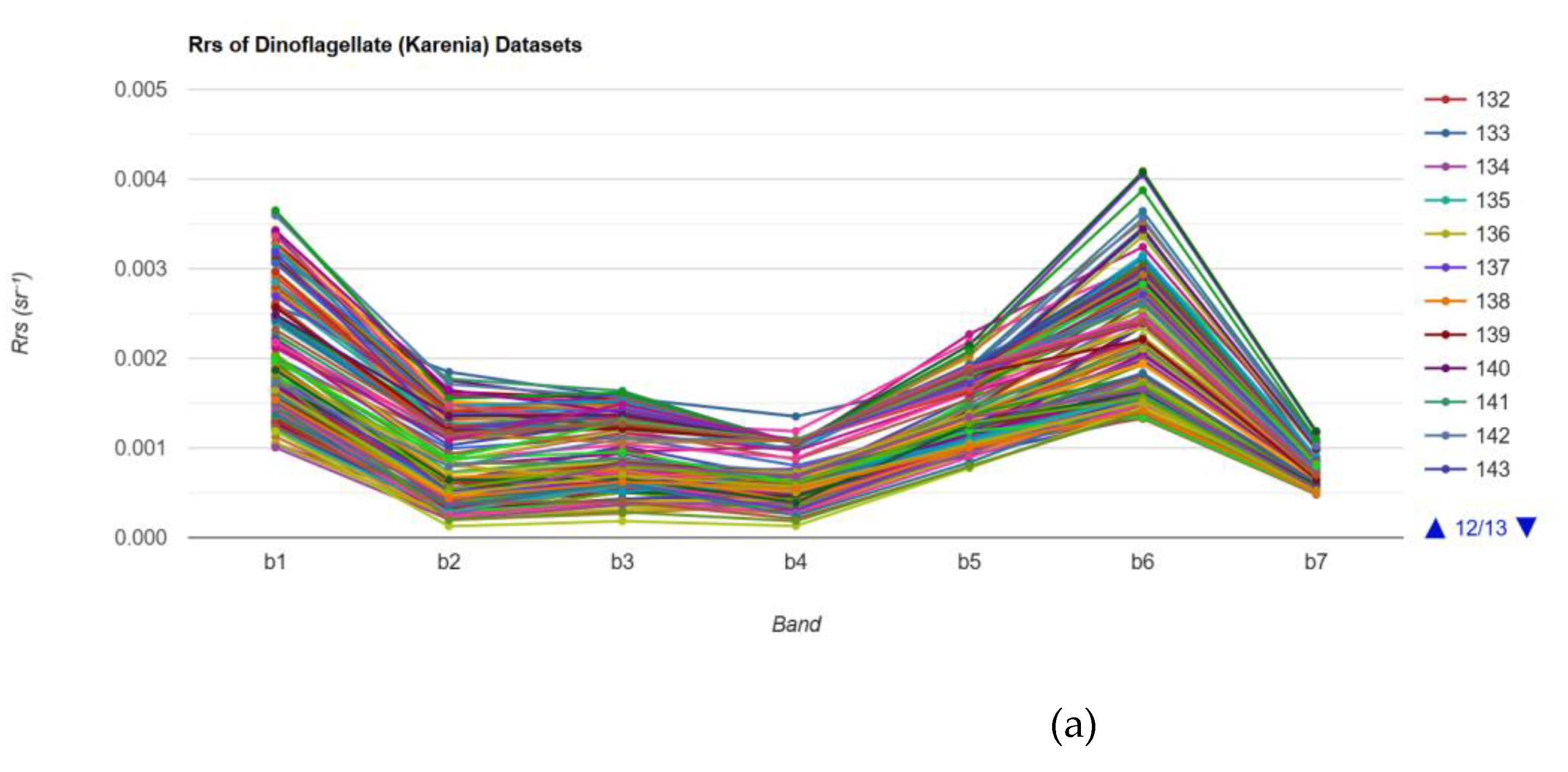
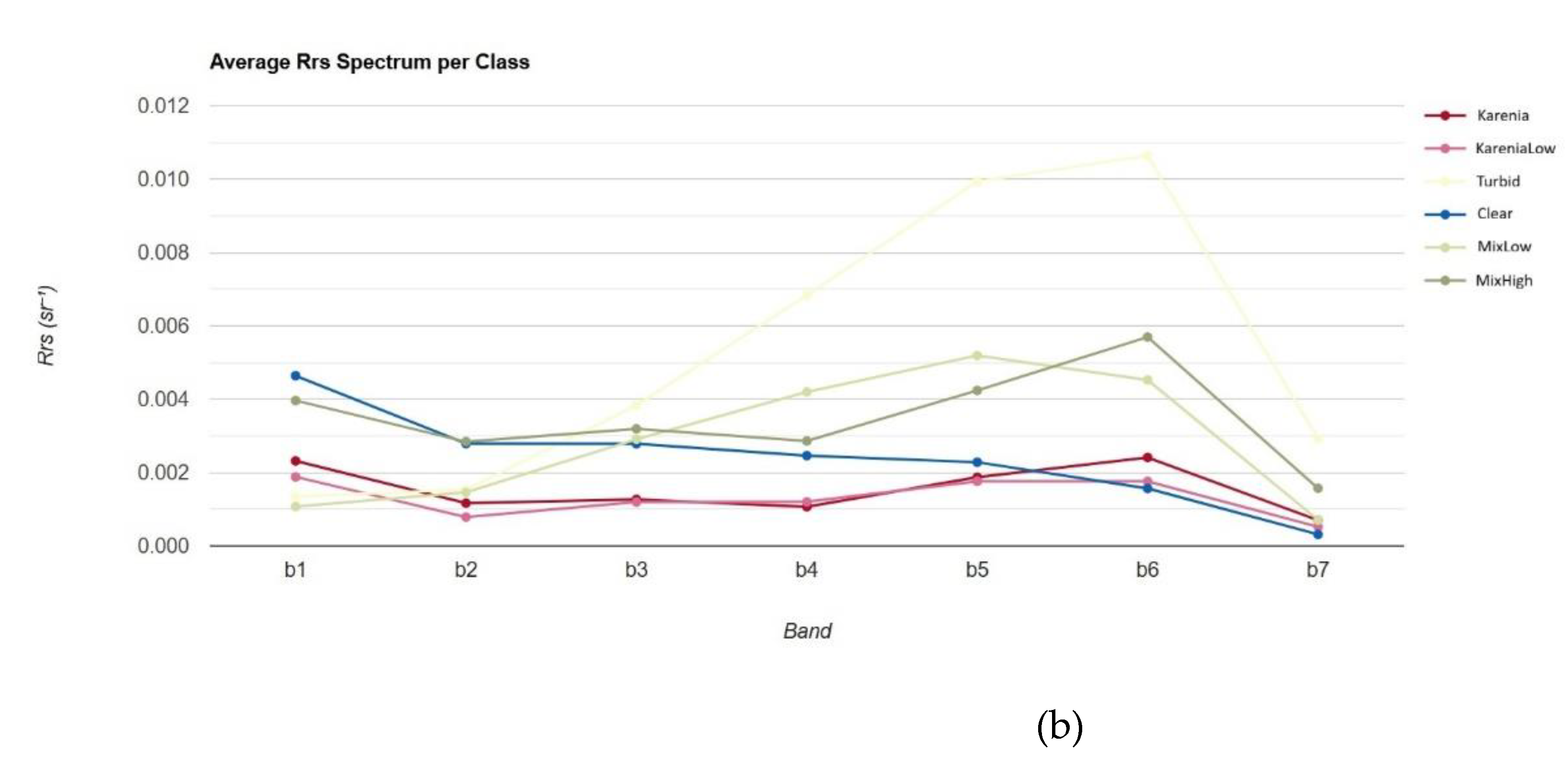
Figure 9.
Diatoms classification results with some scenarios. (a) SGLI data, (b) Classification results using RF with seven bands as the inputs, (c) Classification results using RF with six bands as the inputs, (d) Classification results using CART with seven bands as the inputs, and (e) Classification results using GTB with seven bands as the inputs.
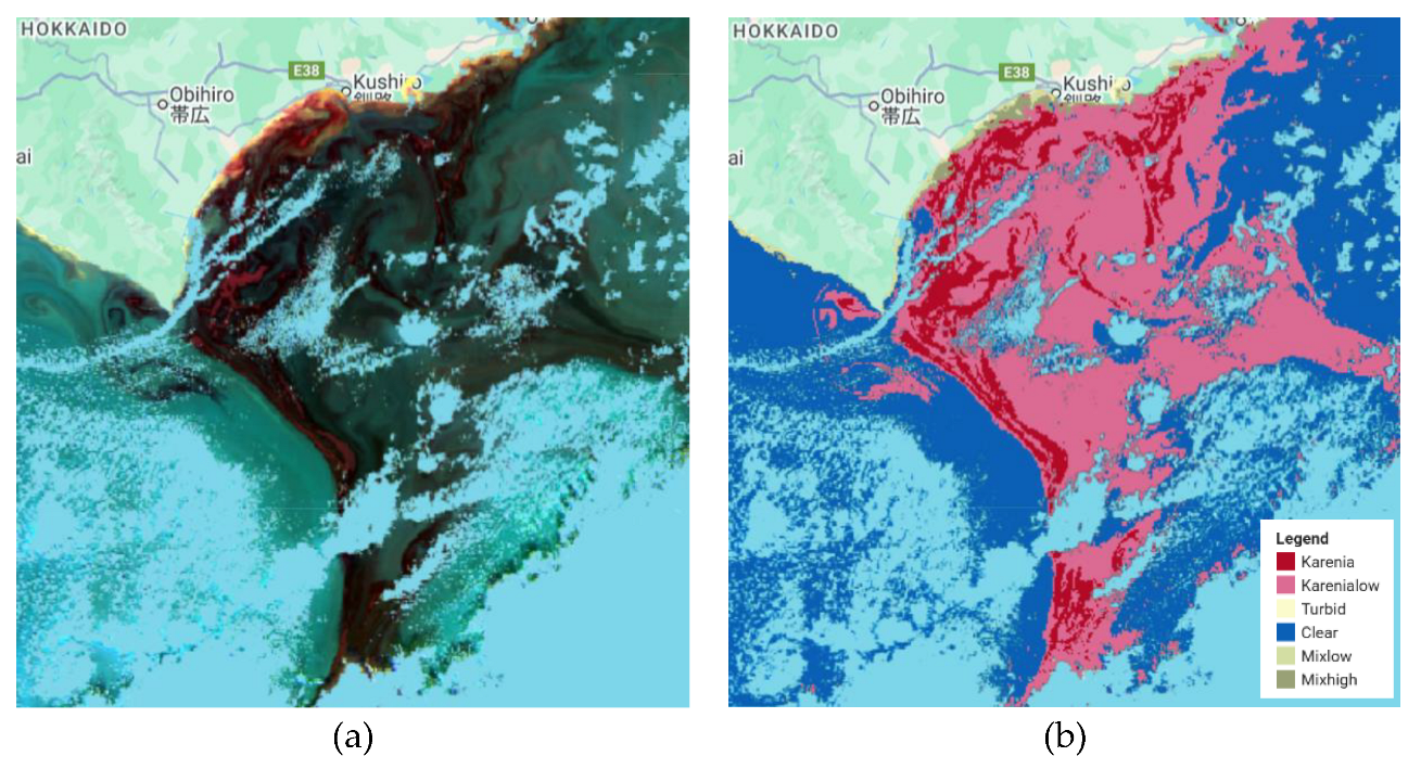
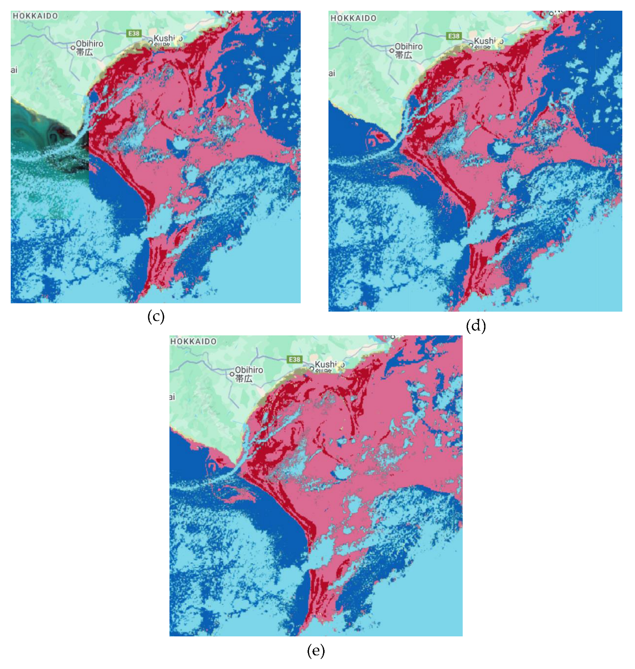
Table 1.
Descriptions of the expected or confirmed optical water and phytoplankton types in different sub-regions.
Table 1.
Descriptions of the expected or confirmed optical water and phytoplankton types in different sub-regions.
| Sub-region | Observation date | Consideration/ confirmation |
|---|---|---|
| Southeastern Indian Ocean | 2 December 2023 | Phytoplankton bloom due to upwelling associated with the 2023 El Niño |
| Malacca Strait | 1 July 2021 | Well-known turbid water [35] |
| East China Sea | 30 January 2021 | Well-known turbid water especially in winter due to intense wind- driven vertical mixing [36] |
| Bohai Sea | 30 January 2022 | Well-known turbid water especially in winter due to intense wind- driven vertical mixing [37] |
| Yellow Sea | 30 January 2022 | Well-known turbid water especially in winter due to intense wind- driven vertical mixing [37] |
| Tokyo Bay | 17 July 2023 | Well-known to be optically complex water attributed to riverine effluent rich in CDOM [38,39] |
| Sagami Bay | 17 May 2020 | Confirmed phytoplankton coccolithophore bloom [40] |
| Southeast Hokkaido | 13 October 2021 | Confirmed red tide caused by phytoplankton from the dinoflagellate group [41,42] |
| 8 May 2022 | Expected to be seasonal blooms of phytoplankton diatom | |
| 7 May 2022 | Expected to be seasonal blooms of phytoplankton diatom |
Table 2.
Accuracies of the results.
| Scenario | Overall Accuracy | Kappa Coefficient |
|---|---|---|
| RF with seven bands | 0.975609756097561 | 0.9622119815668202 |
| RF with six bands | 0.9391304347826087 | 0.9105555555555555 |
| CART with seven bands | 0.967479674796748 | 0.9496520671305773 |
| GTB with seven bands | 0.983739837398374 | 0.9749056411302665 |
Table 3.
Accuracies of the results.
| Scenario | Overall Accuracy | Kappa Coefficient |
|---|---|---|
| RF with seven bands | 0.9775280898876404 | 0.9687719298245613 |
| RF with six bands | 0.9642857142857143 | 0.9503154574132492 |
| CART with seven bands | 0.9662921348314607 | 0.9532317393589069 |
| GTB with seven bands | 0.9775280898876404 | 0.9687719298245613 |
Disclaimer/Publisher’s Note: The statements, opinions and data contained in all publications are solely those of the individual author(s) and contributor(s) and not of MDPI and/or the editor(s). MDPI and/or the editor(s) disclaim responsibility for any injury to people or property resulting from any ideas, methods, instructions or products referred to in the content. |
© 2025 by the authors. Licensee MDPI, Basel, Switzerland. This article is an open access article distributed under the terms and conditions of the Creative Commons Attribution (CC BY) license (http://creativecommons.org/licenses/by/4.0/).
Copyright: This open access article is published under a Creative Commons CC BY 4.0 license, which permit the free download, distribution, and reuse, provided that the author and preprint are cited in any reuse.


