
Submitted:
04 January 2024
Posted:
05 January 2024
You are already at the latest version
Abstract
This paper aims to quantify the influence of hydrogen embrittlement on Wierzbicki and Xue (W-X) model parameters. This model has 4 parameters which have been obtained by tensile tests on smooth specimens, tensile notch specimens, single notch tensile specimens (SENT) and pure shear specimens. Hydrogen embrittlement has been obtained by electrolytic method. Application of the (W-X) model has been done to get the local resistance used to predict failure by the Volumetric Method (VM). An example is given for the case of an embedded pipe submitted to service pressure and lateral seismic displacement. The effect of this displacement is then assimilated to the shearing of the straight section of the pipe. The pipe shows a corrosion defect considered a semi-elliptical crack. The influence of hydrogen embrittlement on local strain resistance and safety factors is discussed.
Keywords:
W-X plasticity model
; Hydrogen embrittlement
; pipe failure
; seismic displacement
; safety factor
1. INTRODUCTION
Degradation of overtime of the properties of the materials by hydrogen is called hydrogen embrittlement (HE). Fracture toughness and failure elongation are reduced. It has little influence on yield strength and ultimate strength. Johnson [1] discovered this phenomenon at the end of the 19th century.
For the transport of blended hydrogen, the degradation depends on the concentration, the exposure time and the service pressure. The introduction of hydrogen in the natural gas network needs also to pay attention to hydrogen permeation because of the low ignition energy and large flammability range of hydrogen. More attention to pipe integrity surveillance and maintenance is therefore necessary [2,3].
A loss of ductility and reduction of fracture resistance characterize the hydrogen embrittlement as can be seen in Figure 1.
The pipe failure risk increases by hydrogen embrittlement. Solutions for risk reduction include lowering the design factor, identifying fracture toughness under HE to know the safety factor, developing integrity and surveillance plans, and the modification of the operating pressure conditions. The optimal solution includes pipeline transport capacity requirements, the status of existing pipelines, and trade-offs between capital and operating expenditure
HE has been widely described in the literature [4,5,6]. Hydrogen is transported into metals by diffusion after the dissociation of molecular hydrogen at the surface. Hydrogen transport is also made by dislocations. Several mechanisms are invoked to explain HE namely:
- weakening of metal-metal atomic bonds
- modification of plasticity,
- decohesion / dislocation competition
- molecular recombination on defects,
- stress triaxiality.
- weakening of metal-metal atomic bonds
- modification of plasticity,
- decohesion / dislocation competition
- molecular recombination on defects,
- stress triaxiality.
The stress triaxiality β has a strong influence on the failure strain [7,8,9]. It decreases exponentially with triaxiality according to:
Ductile failure mechanisms consist of the nucleation, growth, and coalescence of micro-voids under a high-stress triaxiality. Under low-stress triaxiality, the mechanism of ductile fracture is different and consists of a shear band and instability, Figure 2. The failure mechanism depends on both of the stress triaxiality β and shearing whose intensity is given by the Lode angle . Bai-Wierzbicki [10] has proposed a ductile fracture criterion in the space where the fracture strain is a function of the stress triaxiality β and the Lode angle . Bai-Wierzbicki [10] introduces the stress triaxiality β and the Lode angle to transform the Mohr–Coulomb model. This approach is now widely used for the problem of pipe failure [11,12,13,14,15,16,17,18,19].
The model parameters are calibrated from experimental fracture tests covering a wide range of stress states. The smooth round bar tension test, notched round bar tension test, plate tension test and bending tension test are used to obtain positive stress triaxiality. Torsion and notched tube tension tests give fracture with nearly zero stress triaxiality. Cylindrical compression tests are used for negative stress triaxiality.
The influence of the stress triaxiality β and the Lode angle is important for the Local Strain Based Design concept through the local effective strain.
In the presence of a defect, the strain distribution at its head exhibits a gradient. The failure criterion is based on
The effective local strain demand is related to particular conditions of stress triaxiality β and loading through the Lode angle . The local strain resistance is obtained from the distribution of the tensile failure strain corrected according to the model of Wierzbicki and Xue (W-X) [9]. The failure strain measured by a tensile test is obtained under specific conditions (β = 0.33 -).
The influence of hydrogen embrittlement on Wierzbicki and Xue (W-X) parameters is studied in the following. This model has 4 parameters which have been obtained by tensile test on smooth specimens, tensile notch specimens, single notch tensile specimens (SENT) and pure shear specimens. Hydrogen embrittlement has been obtained by the electrolytic method. Application of the (W-X) model has been done to get the local critical resistance used to predict fracture by the Volumetric Method (VM) [20]. An example is given for the case of an embedded pipe submitted to service pressure and lateral displacement. The effect of this displacement is then assimilated to the shearing of the straight section of the pipe. The pipe shows a semi-elliptical crack-like defect.
2. WIERBIECKI AND XU FAILURE STRAIN CRITERION
In the X-W plasticity model, it is assumed that failure strain is influenced by the stress triaxiality of the β and Lode angle θL. These two parameters affect independently the local failure strain according to:
is the local reference strain for a zero value of the stress triaxiality and the Lode . The ratio of the hydrostatic stress and the equivalent stress defines the stress triaxiality:
The function gives the stress triaxiality dependence:
C and D are material constants. The dependence with the Lode angle is given by:
where is defined as the ratio of the failure strain between the generalized shear and the generalized traction ( subjected to the same hydrostatic pressure. k is a constant taken equal to unity.
The lode angle is given by :
where are the principal stresses, is the third invariant of the stress tensor and the Von Mises equivalent stress.
3. MATERIAL AND HYDROGENATION METHOD
The pipe steel, API 5L X60 is studied in this paper. Table 1 shows the chemical composition of this micro-alloyed steel. The carbon content is 0.16% . Few additions of alloying elements, such as titanium and niobium are indicated in the chemical composition of Table 1.
The mechanical properties are: yield stress σy = 510 MPa, ultimate strength σul= 610 MPa, and elongation at failure A% = 21%. The influence of hydrogen embrittlement (HE) is seen in Figure 3. The yield stress and the ultimate strength are few affected by HE. One notes a strong reduction of the failure elongation (25%) after HE
The hydrogenation of the specimens is carried out via an electrochemical cell shown in Figure 4. The cell divides into two parts. The first part consists of a basin of NS4 (Natural Soil 4) prepared using demineralized water and an analytical reagent. The specimen is immersed in this basin and is connected to a potentiostat via a copper wire soldered on its non-useful part. In this same basin, an auxiliary platinum sheet electrode is used to apply a constant cathode potential during the test. To ensure that the NS4 solution maintains a neutral pH, nitrogen (N2) and carbon dioxide (CO2) are added throughout the experiment.
The second beaker contains a solution of potassium chloride (KCl), and a saturated Calomel electrode (ECS) serving as a reference for measuring the corrosion current.
The electrical junction between the two containers is done via an Agar/Agar type salt bridge. Finally, to ensure the weakening of steel only in the useful area of the specimen, epoxy paint is used on the non-useful area to protect it from hydrogen.
The registration of the cathodic polarisation current allows to control the hydrogen-charging process is controlled by. Equation (9) gives the quantity of hydrogen on the metal surface :
The hydrogen discharging process under anodic polarisation is used to determine the hydrogen concentration in metal with the use of the method proposed in the work [21]. The standard three-electrode electrochemical cell has been used. According to the recommendation of [21], the hydrogen discharging of the specimen is carried out in 0.2 M NaOH (pH=12.4) solution under anodic polarisation during some defined time. The total quantity of absorbed hydrogen by metal can be defined as:
where is an anodic polarisation current for hydrogen charged specimen and is the anodic polarisation current for a specimen without hydrogen (reference curve); Calculation of hydrogen concentration was done according to the formula:
where z is the number of electrons taken in reaction; F is the Faraday constant; is the effective volume of the specimen This volume is the volume of the active area of the specimen (not cover with painting)and is simply the product of the length by the width and by the thickness of the parallelepiped volume.
. After 120 hours of electrochemical charging, the hydrogen concentration is about
4. IDENTIFICATION OF THE MODEL PARAMETERS
The Xu and Wierbiecki failure strain criterion has four material constants. The parameters C and D are related to the dependence with the stress triaxiality . The parameter . is the local reference strain for a zero stress triaxiality and a Lode angle equal to zero.
Tensile tests on Double Edge Notch Tensile specimens (DENT) are performed to identify parameters C and D. DENT specimens have four different notch radii [ 0.1; 0.25; 0.5 ; 0.75 mm] are used. The geometry of these specimens is reported in Figure 5 and their failure elongations in Table 2. The stress triaxiality has been computed according to the Bridgman formula. [22]. The mean value is obtained from three identical tests performed in with and without HE.
Figure 5.
Geometry of the DENT specimens.
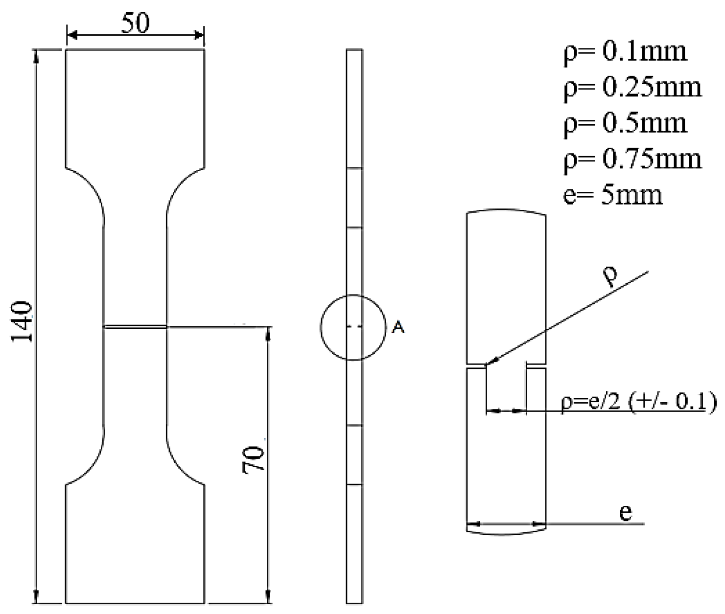
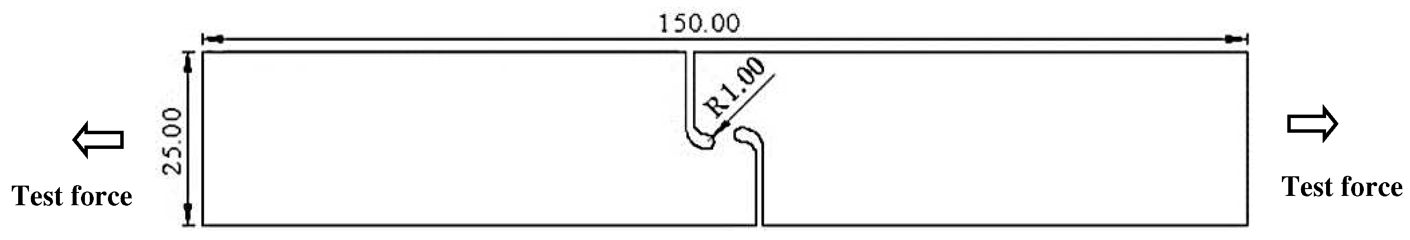
Figure 6.
Geometry of the pure shear specimen.
The dependence with the stress triaxiality is given in Equation 12 for tests performed without HE:
For tests with HE, in Equation 13 :
The value of the D parameter is: D =1.44 (tests performed without HE) and close to the value generally found in literature [10,11,12,13]. For the test performed after HE, the value of the D parameter is less. No comparison with literature values is possible. Evolutions of failure elongation on DENT specimens are presented in Figure 7.
Two tests are used to obtain The material constant (equation 6). The first test gives the shear elongation at failure , and the second the tensile elongation at failure . The parameter is given by the ratio of these two failure elongations:
The geometry of the pure shear specimen is given in Figure 6; The values of the parameter are given in Table 3.
Effective strain resistanceis obtained from W-X model with k=1. The elongation at failure in tension is a particular case of effective strain resistance.
With the values of these constants the values of the reference local strain are : and
5. EFFECTIVE STRAIN FAILURE CRITERION
Implantation of pipelines in severe conditions induces Strain-Based Design (SDB). Strain-Based Besign (SDB) is applied when displacement-controlled loads are the predominant design conditions. In addition to the internal pressure, seismic activity, soil subsidence, slope instability, frost heave, thermal expansion and contraction, landslides, pipe reeling, pipe laying, and other types of environmental loading produce large stress and strain in the pipe wall. The use of steel having a large strain hardening capacity and sufficient plastic deformation is necessary.
The basic equation for SBD compares the applied strain or strain demand εD with the permissible strain or strain capacity εc :
The strain capacity is defined as :
fs is a safety factor and the failure elongation.
The presence of a defect in a structure or component induces a non-uniform strain distribution of deformations at its head as a consequence of the presence of a hot spot. The Strain Based Design concept must be adapted to the Local Strain Based Design as equation (18) at the local level (LSBD). The failure criterion is based on:
The local effective failure strain is obtained with particular conditions of stress triaxiality β and loading through the Lode angle .is the local strain resistance.
Failure needs energy which is assumed to be stored in a Failure Process Volume. Several approaches are available and generally reduce this volume to a cylinder in order to have a 2D approach. The different 2D models are based on plastic zone size, material parameter notch geometry or stress or strain distribution.
Among then, the Volumetric Method (VM) [20] is based on the inflexion point on the stress distribution. This inflexion point is determined at the minimum of the relative stress gradient
where and are the relative stress gradient and maximum principal stress or crack opening stress, respectively.
An example of the strain distribution at a corrosion defect tip in a pipe submitted to internal pressure and lateral displacement is given in Figure 8. From this distribution, the effective strain according to (VM) procedure is obtained and plotted as a function of the distance in front of the tip of the defect. The effective distance Xef is determined at the position where the relative stress gradient is minimum. The effective strain corresponding to the local strain demand value is obtained from the average value on the strain distribution over the effective distance. The obtained value εef is introduced to the concept of the local strain failure criterion.
6. APPLICATION : EMBEDDED PIPE EXHIBITING A DEFECT SUBMITTED TO INTERNAL PRESSURE AND EXTERNAL DISPLACEMENT
6.1. loading conditions
A pipe made in API 5L X60 steel with a diameter of 610 mm and a thickness of 11 mm is submitted to the following three loads:
- the pipe is completely embedded in soil with a ground reaction coefficient of 100MN/m3,
- the internal pressure of the pipeline is 70 bars,
- it is also subject to a local seismic displacement Δ which depends on the amplitude of an earthquake M (Richter scale) according to :
With Δ corresponding to the rounding of the median value of the mean displacement after an earthquake resulting from the correlations of Wells and Coppersmith [23].
This local displacement is assumed to be superimposed at an equal distance between two enclosed ends. This distance is assumed arbitrarily equal to 13 m.
The pipe shows a crack-like defect at 3 hours with depth d = 1.7 mm and aspect ratio c/e = 18.5/31 = 0.59 where c is the width and e is the length of the semi-axis of the defect.
The displacement is imposed on the level of the semi-elliptical defect as the least favourable conditions. The effect of the earthquake is then assimilated to a shearing of the straight section of the pipe as the most severe conditions, Figure 9.
Local strain is computed from FEM by imposing displacement Δ. To compute the local strain demand resulting from the local displacement, the pipe and the defect were meshed with 3D hexahedral elements. Finite element computing was performed using Abaqus software.
The model considered is a deformable 3D solid, taking up the assumptions and sizes mentioned above. The mesh elements are quadrangle and were generated using the transformation algorithm. The average size of the elements is 13mm except at the level of the defect where it is 2mm, Figure 10. A mesh analysis was carried out to ensure that no element was distorted and thus limit the loss of information during the simulations.
The steel mechanical properties are : Young's modulus of 210 GPa, Poisson's ratio of 0.3 and density of 7.8 kg/m3.
6.2. Results
FEM computes the effective local strain as strain demand, the stress triaxiality and the lode angle at the effective distance of the strain distribution Xef in the direction of maximum opening stress versus displacement Δ. The results are presented in Table 4.
The evolution of the effective local strain versus the displacement Δ is presented in Figure 11.
One notes a linear relationship between the effective local strain and the displacement Δ after a transient state when the displacement is less than 20 mm.
Beyond this value, the displacement is the most important loading mode when comparing with internal pressure and soil reaction.
The effective local strain corresponds to the strain demand which is compare to the strain resistance. This local strain resistance is obtained from the original X-W criterion with a small modification :
With E =C. Values of the W-X parameters are presented in Table 5 for test without HE and with HE. Original data are presented in Table 3.
Figure 12 shows the evolution of the local strain resistance versus the displacement Δ. For small displacements in the range [4,5,6,7,8,9,10,11,12,13,14,15,16,17,18,19,20] mm, the relative difference between local strain resistance without HE and with HE is in the range [20%-9%], the local strain resistance without HE is higher. One notes that the failure elongation in pure tension after HE is decreasing of 25%. For higher displacement, the relative difference decrease rapidly with displacement Δ.
It is less than 1% for displacement higher than 52 mm. One concludes that the loss of ductility is strongly more important when due to the stress triaxiality and the Lode angle than due to the hydrogen embrittlement. However, this loss of ductility is important when comparing with local strain resistance with failure elongation in pure tension.
Design is based on a safety factor in order to take into account the aleas associated with loading and material resistance. A safety factor fs greater than 22 is recommended.
The ratio the local strain resistance and the effective local strain demand defines the safety factor :
The safety factor with and without hydrogen embrittlement versus displacement Δ is reported in Figure 13.
One notes a strong decrease of the safety factor with the displacement Δ. The safety factor for the steel pipe without hydrogen embrittlement is always higher that the safety factor after HΕ. The relative difference decreases with the increase of the displacement; 20% for Δ =4 mm and 9% for Δ=20mm. In Figure 13, the displacement is limited to 20 mm because beyond this value the two safety factor are less than 2 and are not admissible for the safety of the pipe. In the displacement range [4 mm-20 mm], the safety factor ratio vary in the range [1.25-1.10].
7. DISCUSSION
This paper uses the concept of Local Strain Based Design for the computing of the safety factor of a pipe exhibiting a crack-like defect and submitted to a multi-loading (soil reaction, internal pressure, lateral movement). The reason of this choice can be found on the historical point of view on the evolution of the concept which is summarize as follow. If we consider the pipe with the presence of a semi-elliptical defect, the introduced surface discontinuity subjected to loading will produce a variation in potential energy which in the absence of dynamic effects will be balanced by the energy expenditure of surface creation. The strain energy stored and used in the crack extension will be contained in the volume of the fracture process. For simplification, this will be assimilated to a cylinder of height the thickness of the pipe and diameter a quantity called the characteristic distance.
This concept of characteristic distance was firstly introduced by Irvine and Quirk [24] who assumes that at the head of a strain concentration, the stress is uniform over the characteristic distance and equal to ultimate strength.
Guillemot [25] assumes that the fracture energy is identical to the failure energy of a micro tensile specimen of length l0. This fracture energy density depends on yield stress, ultimate strength and elongation to failure because it is related as the area of the stress-strain curve. The earlier approach considers that the local material resistance is identical to the tensile failure resistance. In addition, the characteristic distance is independent of the loading mode and component geometry.
Griffith and Owen [29] consider that the failure mechanism is ruled by the maximum plastic strain located at the notch tip. This maximum plastic strain is strongly dependant of the notch radius.
The ductile fracture can be divided in three steps:
- void nucleation,
- void growth,
- final instability of the ligament between voids.
Osborne and Embury [27] have first consider that the local failure strain is not the same that the failure elongation in tension but those obtained in plane strain tension.
Rice and Tracey [7] have shown that the growth rate of a spherical cavity in a perfectly-plastic materials depends exponentially of the stress triaxiality. Barnby and al [28] proposed a relationship where the critical void radius depends linearly of the stress triaxiality.
A general description of the influence of the stress triaxiality and loading mode is given by the Wierzbicki and Xue [9] model. The shear-tension ratio is described by the Lode angle. Therefore the use of a Local Strain Based Design approach derives from evolution of the ideas on ductile failure at a strain concentration. This new approach takes into account the fact that the critical local strain is sensitive to stress triaxiality and Lode angle and the effective distance sensitive to loading mode and geometry through the constrain factor.
Figure 14 compare the failure strains for, i) a smooth, ii) a notched specimen, iii) the local failure strain at the defect tip for a displacement Δ of 4 and 20 mm. One note that the local failure strain and the (gross) failure strain of a notched specimen are similar as well their stress triaxiality. The difference with and without HE is very small which confirms the major influence of stress triaxiality and the secondary one of HE
One notes a strong decrease of the failure elongation with stress triaxiality and lode angle. This is illustrated in Figure 15 where the local strain resistance is reported versus the stress triaxiality β. For the lowest value of the stress triaxiality, the local strain resistance after HE is 6.5% which is practically 1/3 of the failure elongation in tension after HE. This decrease is supported by the experimental values of Table 2. When comparing with failure elongation in tension without HE, the decrease is more than ¼. An explanation is given by the fact that the stress triaxiality hides the influence of hydrogen embrittlement.
Comparison of tensile failure elongation with and without HE gives a false information of the capacity of the pipe to accommodate the loss of ductility in presence of a sharp defect. For conservative reasons, the studied pipe exhibits a corrosion defect considered as a semi-elliptical crack with depth d = 1.7 mm and aspect ratio c/e = 18.5/31 = 0.59 i.e. a deep defect with a high constraint value. The introduction of a defect penalizes twice. The defect induces a strain concentration and increases the stress triaxiality at the tip of the defect.
The safety factor fs is defined in equation (26). Figure 13 shows that this safety factor is always higher without HE than with HE. The value fs >2, value widely used in many codes, is obtained for displacement less than Δ= 19 mm without HE and 18 mm with HE. For higher values, the safety factor is practically identical with a ratio in the range [1.06-0.995].
It has been assumed that the lateral displacement Δ superimposed to the internal pressure and soil reaction is due to seismic activity. The Gutenberg-Richter (GR) distribution [29] describes the seismic activity according to :
where N(M) is the number of seism of M amplitude during the observation time, a and b are parameters which depend on seismic zone and reference period. The GR distribution law is valid for M < Mmax where Mmax is the maximum amplitude of the earthquake for the considered seismic zone. The parameters of the GR seismic distribution in a high seismic zone are reported in Table 5.
According to equation (27), a displacement of 20 mm is associated with a seism of magnitude 4.5. During a reference period of 50 years about 25 seisms of magnitude greater than 4.5 potentially happen in a high seismic zone. Therefor the risk in a general sense is not negligible and the associated failure probability is Pf = 3,36×10⁻¹. In the same seismic zone and for the same reference period, the failure probability of the same pipe without defect is Pf = 6,89×10⁻². These values are less tan the recommended highest value of a risk probability of 10-5.
Therefore for the transport of pure hydrogen or blended with natural gas, the location of pipelines must avoid urban or semi-urban zones. A strict maintenance policy is necessary.
8. CONCLUSION
We have studied the influence of HE on W-X plasticity model. This influence can be seen by comparing the relative values of the model’s parameters as reported in Table 6.
For the steel API5L X60, the relative values decrease for the parameters D and C of the W-X plasticity model is in the range [12% -32%] after HE.
The parameter incresaes after HE but its’influence is limited because the values of the Lode angle are low (see Table 4). For the studied pipe exhibiting a crack-like defect and submitted to internal pressure, soil reaction and lateral seismic displacement Δ, the local failure strain indicates that for high values of Δ, the effect of HE is hidden by the stress triaxiality effect.
Improvement of the W-X plasticity model is necessary to take into account the thickness and the geometry effects. This can be done by introducing a constrain parameter.
The effect of seismic displacement is severe in terms of failure probability and risks. Therefore, location of pipelines used for hydrogen transport must avoid urban or semi-urban zones. A strict maintenance policy is necessary.
Author Contributions
Conceptualization, G.P. and J.C.; methodology, J.C.; software, L.A.; validation, L.A., J.C. and G.P.; formal analysis, L.A.; investigation, L.A.; resources, J.C.; data curation, G.P.; writing—original draft preparation, L.A.; writing—review and editing, G.P.; visualization, J.C.; supervision, J.C.; project administration, J.C.; funding acquisition, J.C. All authors have read and agreed to the published version of the manuscript.
Nomenclature
| β stress triaxiality |
| δ∗ material constant |
| strain capacity |
| applied strain |
| effective strain |
| local strain failure |
| effective local strain failure |
| failure strain (in tension) |
| shear failure strain |
| failure strain for notched specimens |
| admissible strain |
| local reference strain |
| Lode angle |
| relative stress gradient |
| ) dependence with stress triaxiality |
| dependence with Lode angle |
| hydrostatic stress |
| equivalent stress: |
| principal stresses |
| opening stress |
| σul ultimate strength |
| Δ local seismic displacement |
| A material constant |
| B material constant |
| C material constant |
| hydrogen concentration |
| D material constant |
| F Faraday constant; |
| cathodic polarisation current |
| third invariant of the stress tensor |
| M amplitude of the earthquake |
| Mmax maximum amplitude of the earthquake |
| effective volume |
| Xef effective distance |
| a constant of GR law |
| b constant of GR law |
| c defect semi-axis width |
| d depth of the defect |
| e length of the semi-axis of the defect |
| fs safety factor |
| k constant |
| z number of electrons |
References
- Johnson, W. H. : Proceedings of the Royal Society of London. 1875, 23, 168–179.
- Cabrini M, Coppola L, Lorenzi S, Testa C, Carugo F, Bucella DP, et al. « Hydrogen permeation in X65 steel under cyclic loading. Materials 2020, 13, 2309. [Google Scholar] [CrossRef] [PubMed]
- Wu X, Zhang H, Yang M, Jia, W, Qiu, Y., Lan, L. “From the perspective of new technology of blending hydrogen into natural gas pipelines transmission: mechanism, experimental study, and suggestions for further work of hydrogen embrittlement in high-strength pipeline steels”. Int J Hydrogen Energy. 2022, 47, 807.
- Mohtadi-Bonab, M.A. , Masoumi, M. ”Different aspects of hydrogen diffusion behavior in pipeline steel” J. Mater. Res. Technol. 2023, 24, 4762–4783. [Google Scholar]
- Oriani, R. A ‘‘Whitney award lecture-1987: Hydrogen-the versatile embrittlement. ’’ Corrosion 1987, 43, 390. [Google Scholar] [CrossRef]
- Sofronis, P.; Liang, Y.; Aravas, N. “Hydrogen induced shear localisation of the plastic flow in metals and alloys”. Eur. J. Mech. A/Solids 2001, 20, 857–872. [Google Scholar] [CrossRef]
- Rice, J. R and Tracey.D.M “On the ductile. in triaxial stress fields”. Journal of Mechanics and Physics of Solids 1969, 26, 163–186. [Google Scholar] [CrossRef]
- Mac Clintock, F.A. « A Criterion for Ductile Fracture by the Growth of Holes”. Journal of Applied Mechanics 1968, 35, 363. [Google Scholar] [CrossRef]
- Wierzbicki, T.; Xue, L. Ductile fracture initiation and propagation modelling using damage plasticity theory. Engineering Fracture Mechanics 2008, 3276–3293. [Google Scholar]
- Yuanli Bai. Wierzbicki, T.” A new model of metal plasticity and fracture with pressure and Lode dependence”. International Journal of Plasticity 2008, 24, 1071–1096. [Google Scholar] [CrossRef]
- Zengli Peng, Haisheng Zhao, Xin Li, Lin Yuan, Tong Zhu. “Ductile fracture of X80 pipeline steel over a wide range of stress triaxialities and Lode angles. Engineering Fracture Mechanics 2023, 289, 109470. [Google Scholar] [CrossRef]
- Simiao Yu, Lixun Cai, Di Yao, Chen Bao.3Critical ductile fracture criterion based on first principal stress and stress triaxiality” Theoretical and Applied Fracture Mechanics,10, July, (2020).
- 13. Peihua Han, Peng Cheng , Shuai Yuan, Yong Bai. “Characterization of ductile fracture criterion for API X80 pipeline steel based on a phenomenological approach”. Thin-Walled Structures.
- Bianchetti C., D. Pino Munoz, B. Leble, ouchard P.-O. B. “ Ductile failure prediction of pipe-ring notched AISI 316L using uncoupled ductile failure criteria”. International Journal of Pressure Vessels and Piping 2021, 191, 104333. [Google Scholar] [CrossRef]
- Yajun Zhang, Yuqing Liu, Fei Yang. “Ductile fracture modelling of steel plates under tensile and shear dominated states”. Journal of Constructional Steel Research 2022, 197, 107469. [Google Scholar] [CrossRef]
- Zhao Zhang, Yanqing Wu, Fenglei Huang. “Extension of a shear-controlled ductile fracture criterion by considering the necking coalescence of voids”. International Journal of Solids and Structures 2022, 236–237, 11132. [Google Scholar]
- 17. Oh CK, Kim YJ, Baek JH, Kim YP, Kim WS.” A micro-mechanical model of ductile fracture for API X65 steels and application to pre- strain effects on deformation and fracture. Int J Mech Sci, in press. 2007.
- Xue Yang Yazhou Guo.” A new ductile failure criterion with stress triaxiality and Lode dependence”. Engineering Fracture Mechanics, 5 June, (2023).
- PluvinageG . “Notch effects in fatigue and Fracture”.Editeur Kluwer. (2001).
- Capelle.J Dmytrakh. I &Pluvinage, G. Capelle.J Dmytrakh. I &Pluvinage, G. “Hydrogen effect on local fracture emanating from notches in pipeline with steel API X52”. Problems of Strength. N°5. 401. (2009).
- Bridgman, P. W. “Studies in Large Plastic Flow and Fracture”. McGraw-Hill (1952).
- Wells. D and Coppersmith.K “New Empirical Relationships among Magnitude, Rupture Length, Rupture Width, Rupture Area, and Surface Displacement. Bulletin of the Seismological Society of America 1994, 84, 974–1002. [Google Scholar] [CrossRef]
- Irwine, W. H and Quirk, J.F. “A strain concentration approach to fracture mechanics”. Practical application of fracture mechanics to pressure vessel technology,C2/7, p76-84,London, (1971).
- Guillemot, L. F ”Brittle fracture on welded materials”. Second commonwealth Welding, Conference, London 1965, C7, 353-382.
- Griffith, J. R and Owen, D.R.J Journal of Mechanics and Physics of Solids. 1972, 19, 419. [Google Scholar]
- Osborne, D. E & Embury, J.D” The influence of warm rolling on the fracture toughness of bainitic steels”. Metllurgical and materials transactions B. 1973, 4, 2051–2061. [Google Scholar]
- Barnby, J. T. , Shi, Y.W. & Nadkarni A. S. “On the void growth in C-Mn structural steel during plastic deformation” International Journal of Fracture, volume. 1984, 25, 273–283. [Google Scholar]
- Gutenberg, B. , Richter, C.F.Magnitude and Energy of Earthquakes. Annali di Geofisica 1956, 9, 1–15. [Google Scholar]
Figure 1.
ratio of failure strain H2/air versus yield stress for pipe steels.
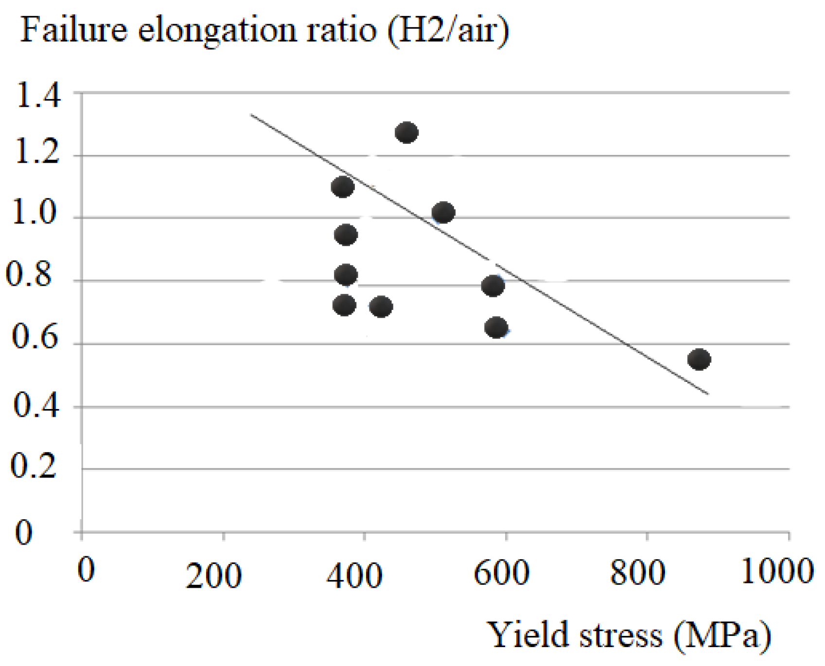
Figure 2.
Evolution of the failure strain with stress triaxiality.
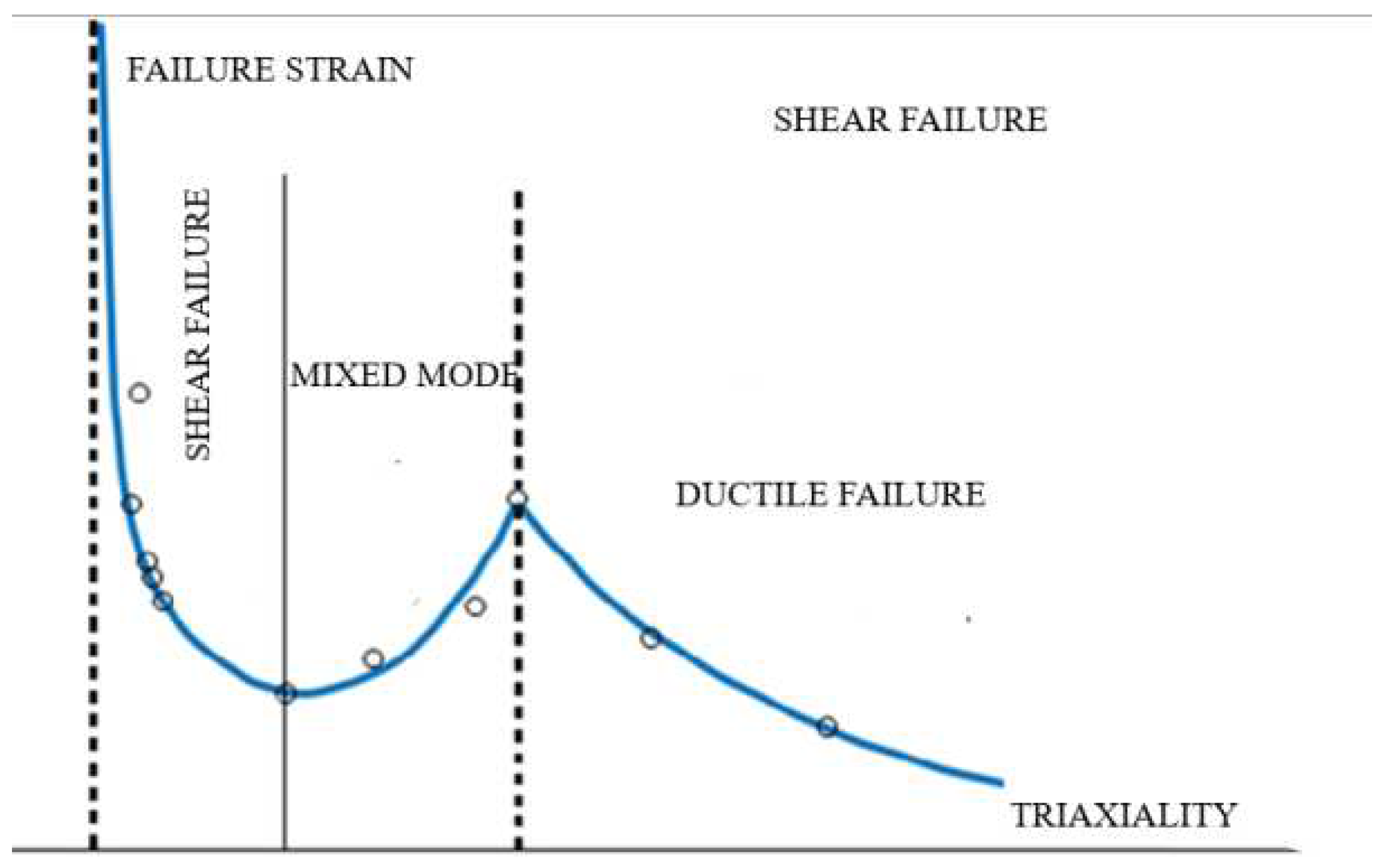
Figure 3.
stress-strain curve of API5LX60 pipe steel with and without hydrogen embrittlement.
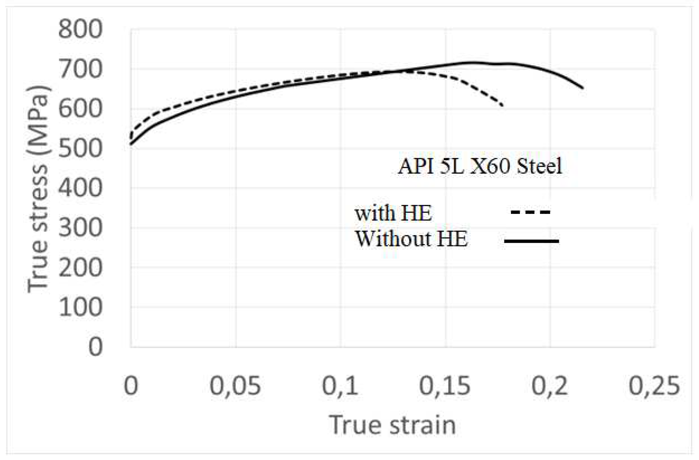
Figure 4.
Explanatory diagram of the cell electrochemical allowing the hydrogenation 1 Specimen; 2. NS4 basin (Natural Soil 4) ; 3.saturated Calomel electrode (ECS) ; 4. platinum sheet auxiliary electrode 5. Agar/Agar type salt bridge.
Figure 4.
Explanatory diagram of the cell electrochemical allowing the hydrogenation 1 Specimen; 2. NS4 basin (Natural Soil 4) ; 3.saturated Calomel electrode (ECS) ; 4. platinum sheet auxiliary electrode 5. Agar/Agar type salt bridge.
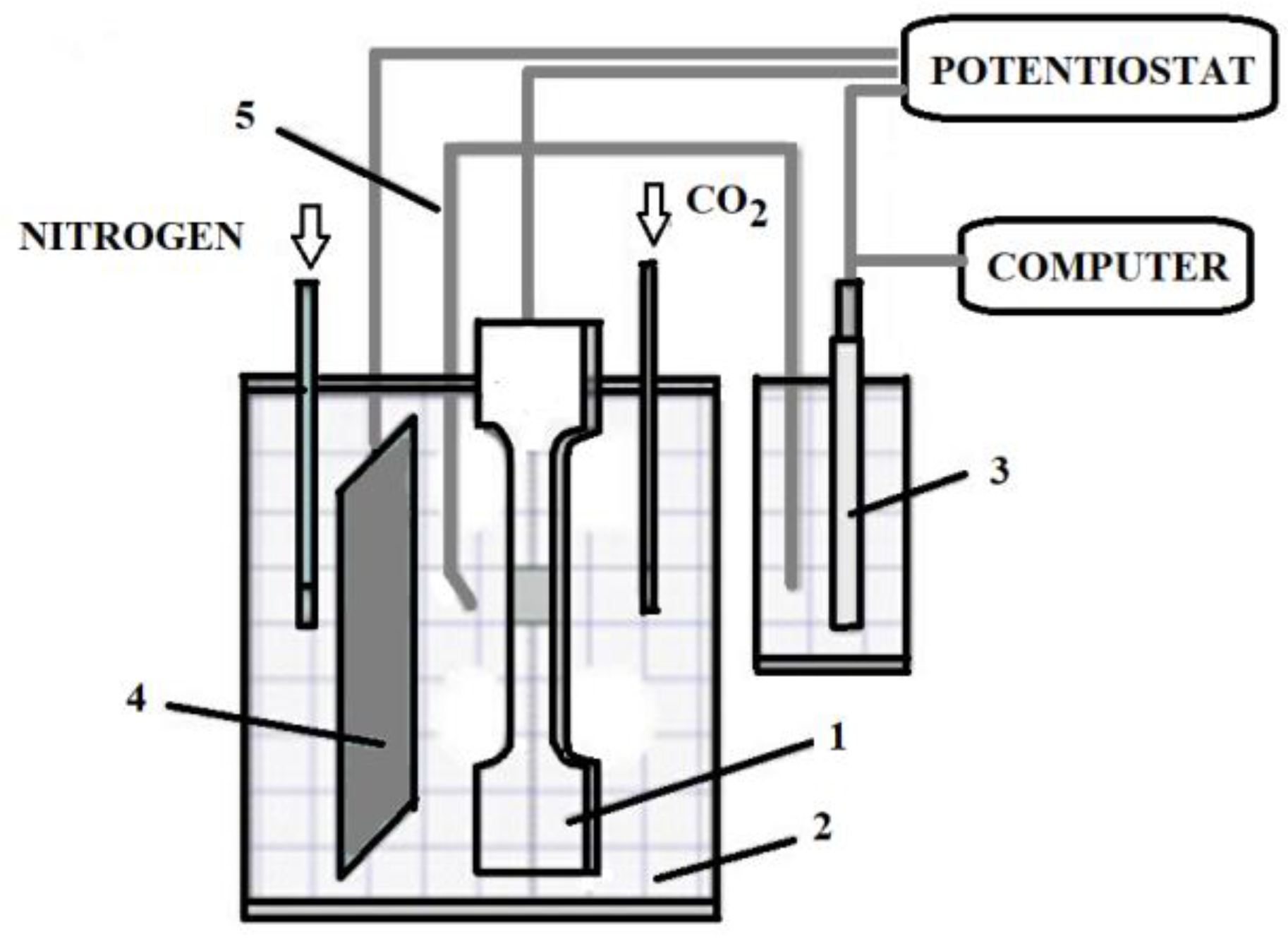
Figure 7.
failure elongation versus stress triaxiality. Tests with and without HE.

Figure 8.
local distribution of strain for a pipe submitted to a lateral displacement of 12.5 mm and internal pressure of 70 bars. Determination of local effective strain by Volumetric Method procedure [20].
Figure 8.
local distribution of strain for a pipe submitted to a lateral displacement of 12.5 mm and internal pressure of 70 bars. Determination of local effective strain by Volumetric Method procedure [20].
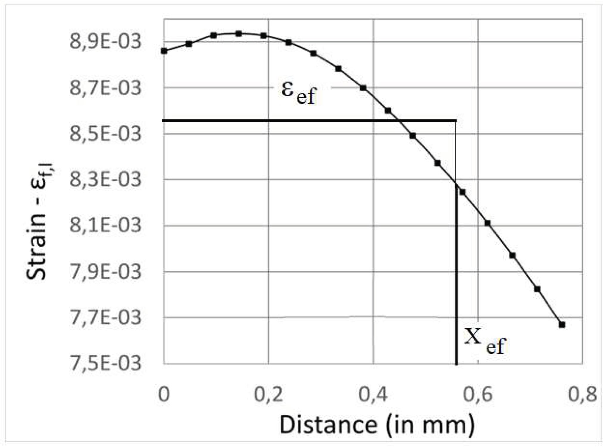
Figure 9.
Diagram showing the modelling assumptions of a pipeline subjected to an earthquake.
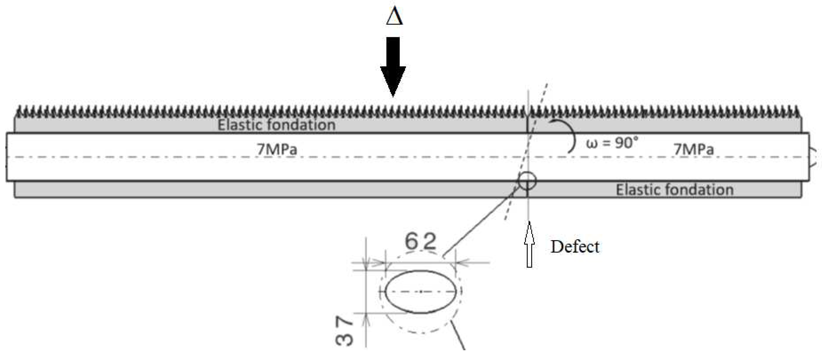
Figure 10.
meshing in the zone near the crack-like defect.
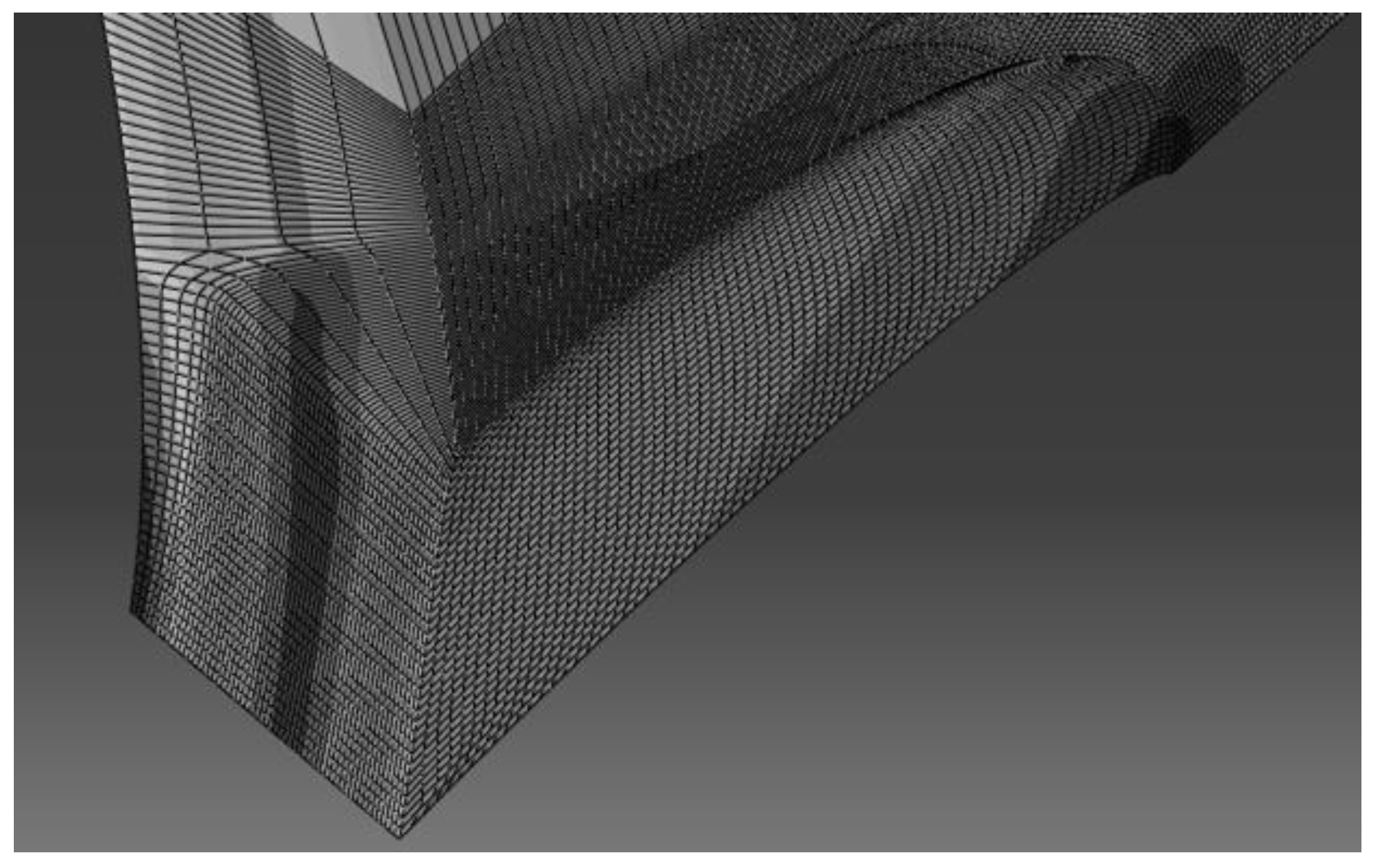
Figure 11.
effective local strain versus the displacement.
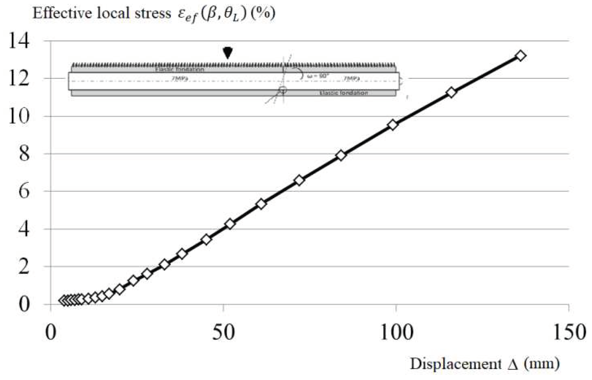
Figure 12.
local strain resistance versus the displacement Δ.
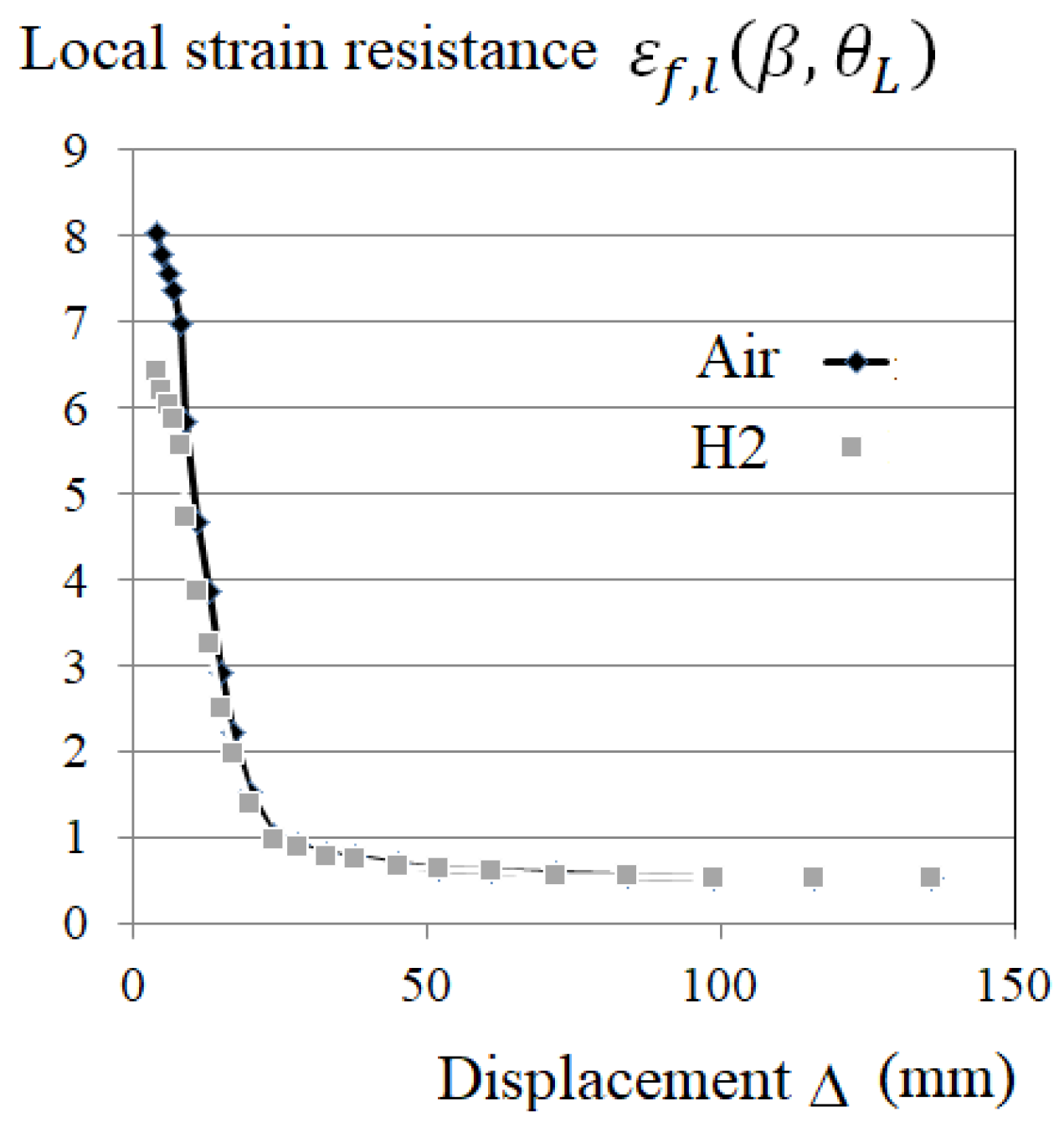
Figure 13.
safety factor fs with and without hydrogen embrittlement versus displacement Δ..
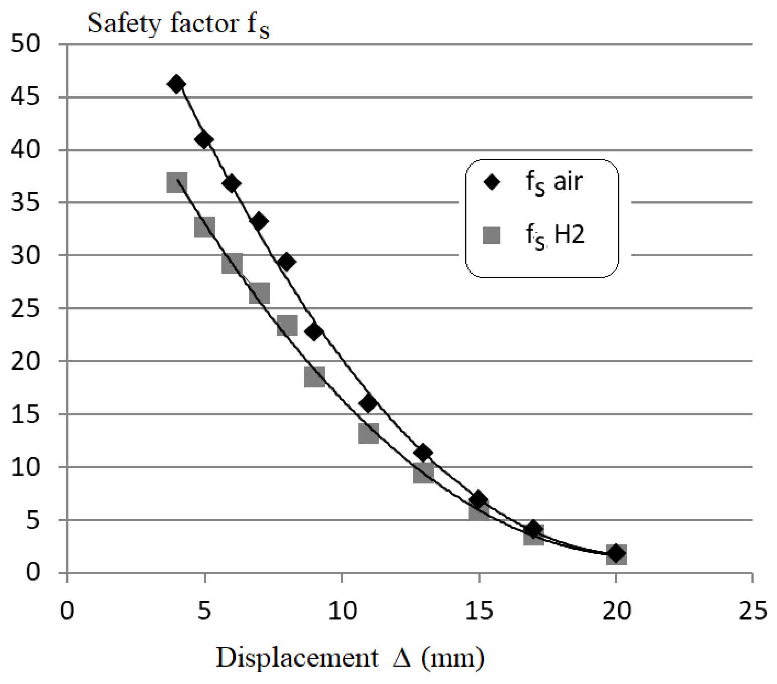
Figure 14.
failure strains of a smooth and a notched specimen and local failure strain for a displacement Δ of 4 and 20 mm.
Figure 14.
failure strains of a smooth and a notched specimen and local failure strain for a displacement Δ of 4 and 20 mm.
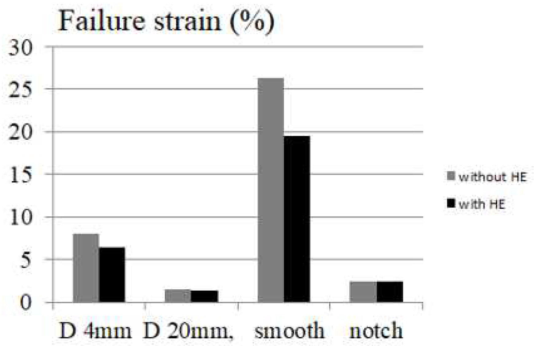
Figure 15.
local strain resistance is reported versus the stress triaxiality.
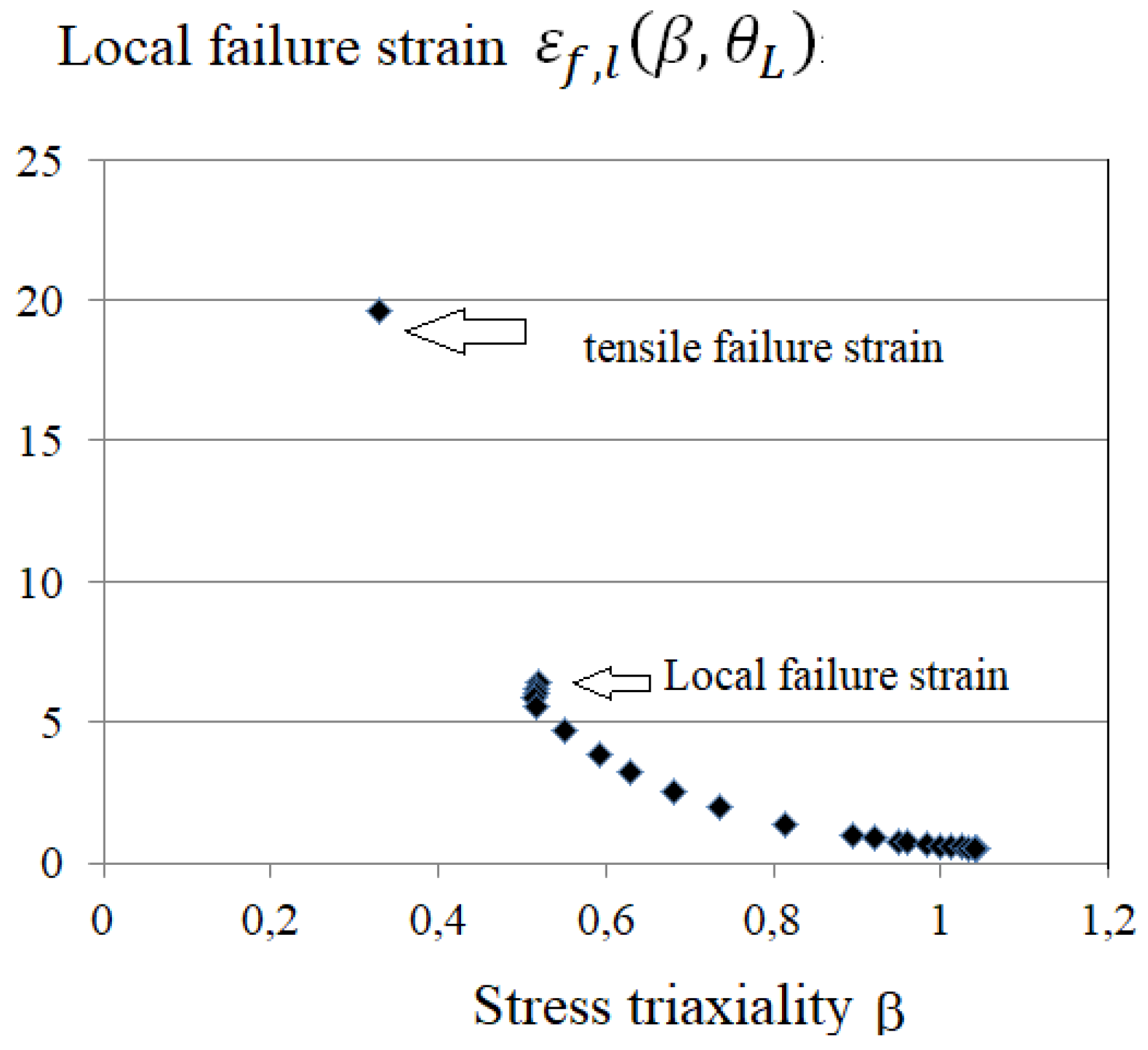

Table 1.
Chemical composition of API 5L X60 steel.
| Additives | C | Si | Mn | P | S | V | Nb | Ti |
|---|---|---|---|---|---|---|---|---|
| % | 0.16 | 0.45 | 1.65 | 0.020 | 0.010 | 0.07 | 0.05 | 0.04 |
Table 2.
Results of fracture tests on DENT specimens made in API 5L X60 steel.
| Notch radius (mm) | (%) air | (%) Hydrogen | Stress triaxiality |
|---|---|---|---|
| 0.75 | 2.40 | 2.47 | 0,98 |
| 0.5 | 2.08 | 1,96 | 0,89 |
| 0.25 | 1.98 | 1.75 | 0,87 |
| 0.1 | 1.87 | 1.57 | 0,8 |
Table 3.
shear and tensile failure elongations and values of .
| (%) | |||
|---|---|---|---|
| Without HE | 6,57 | 29,1 | 0,23 |
| With HE | 6,03 | 19,6 | 0,30 |
Table 4.
the effective local strain, the stress triaxiality and the lode angle versus displacement.
| Δ (mm) | (%) | (rd) | Δ (mm) | (%) | (rd) | ||
|---|---|---|---|---|---|---|---|
| 4 | 0.174 | 0.52 | 0.293 | 24 | 1.237 | 0.896 | 0.116 |
| 5 | 0.19 | 0.518 | 0.274 | 28 | 1.598 | 0.92 | 0.112 |
| 6 | 0.206 | 0.516 | 0.258 | 33 | 2.093 | 0.95 | 0.108 |
| 7 | 0.222 | 0.514 | 0.243 | 38 | 2.664 | 0.961 | 0.106 |
| 8 | 0.238 | 0.518 | 0.227 | 45 | 3.443 | 0.984 | 0.103 |
| 9 | 0.255 | 0.552 | 0.212 | 52 | 4.256 | 1 | 0.1 |
| 11 | 0.291 | 0.593 | 0.194 | 61 | 5.336 | 1.012 | 0.098 |
| 13 | 0.343 | 0.628 | 0.179 | 72 | 6.583 | 1.024 | 0.096 |
| 15 | 0.421 | 0.682 | 0.16 | 84 | 7.915 | 1.034 | 0.094 |
| 17 | 0.541 | 0.737 | 0.146 | 99 | 9.514 | 1.043 | 0.092 |
| 20 | 0.798 | 0.815 | 0.129 | 116 | 11.26 | 1.04 | 0.091 |
Table 5.
values of the W-X parameters.
| E | C | ||
|---|---|---|---|
| air | 90,76 | -1.44 | 0.23 |
| H2 | 56,97 | -0.784 | 0.30 |
Table 6.
Parameters of the GR seismic distribution in a high seismic zone.
| a | b | Mmax |
|---|---|---|
| 2.99 | 0.79 | 6.6 |
Table 6.
influence of HE on W-X plasticity model parameters.
| parameters | D | C | f | f,s | |
|---|---|---|---|---|---|
| Relative valuewith/without HE | 0.62 | 0.88 | 1.30 | 0.67 | 0.91 |
Disclaimer/Publisher’s Note: The statements, opinions and data contained in all publications are solely those of the individual author(s) and contributor(s) and not of MDPI and/or the editor(s). MDPI and/or the editor(s) disclaim responsibility for any injury to people or property resulting from any ideas, methods, instructions or products referred to in the content. |
© 2024 by the authors. Licensee MDPI, Basel, Switzerland. This article is an open access article distributed under the terms and conditions of the Creative Commons Attribution (CC BY) license (http://creativecommons.org/licenses/by/4.0/).
Copyright: This open access article is published under a Creative Commons CC BY 4.0 license, which permit the free download, distribution, and reuse, provided that the author and preprint are cited in any reuse.


