
Submitted:
30 December 2023
Posted:
03 January 2024
You are already at the latest version
Abstract
This article is devoted to overcoming the contradiction between the problem of maximizing the extraction of wind energy as the goal of optimizing wind turbines, and the use of traditional methods based on criteria for the aerodynamic quality of the blades. A modified technique is considered in which the optimization criterion is the directly extracted flow power. It is based on pulse theory methods that use specific power as an optimization criterion. A comparative analysis of the energy efficiency of different types of turbines is carried out, and the effects of blade inversion are considered. A method for calculating multi-rotor turbines based on the concept of uniform power distribution is presented. The compatibility of proprietary and traditional methods is considered by comparing the results of numerical experiments with calculated and experimental data from sources. Optimization computational algorithms generate data from numerical experiments and determine optimal parameter configurations for the turbines under consideration. It is shown that orthogonal Darrieus turbines in high-speed mode provide energy efficiency comparable to collinear turbines, and multi-rotor turbines with power uniformly distributed over the working section are not inferior in energy efficiency to basic turbines, with linear blade velocities halved.
Keywords:
collinear
; orthogonal
; modified
; power
; criterion
; optimization
; uniform distribution
; multi-rotor
1. Introduction—Subject of Study
The foundation of the world's wind power plant fleet consists of bladed turbines that transform the kinetic energy of the forward airflow into the operation of rotating electric generators, pumps, compressors and other power devices. More than 90% of wind power plants are equipped with turbines featuring a horizontal axis of rotation oriented parallel to the airflow (Figure 1). For the purposes of this study, such turbines are classified as collinear.
Turbines can be made with a different number of blades: from single-blade with counterweights to multi-blade configurations numbering dozens of blades (Figure 2). The most common turbines have three blades.
Relatively recently, in the second half of the twentieth century, the development of vertical-axial installations—where the main axes of turbines are perpendicular to the airflow—has significantly intensified. This allows the classification of such turbines as orthogonal (Figure 3).
The designs of orthogonal turbines are very diverse. Figure 4 shows their most common designs.
The lag in developing orthogonal wind turbines is associated not so much with their conceptual shortcomings but with historical circumstances. The configuration features of collinear (propeller) turbines made it possible to use the achievements of rapidly developing aviation technology, in particular in the field of designing wings, blades, transmissions and attitude control systems. Orthogonal turbines were invented later than collinear ones, and the volume of theoretical research into fundamentally new issues of rotor aerodynamics and the experience in the development and operation of these turbines is much less than that of collinear ones.
The objects of this study are bladed wind turbines. Setting the optimization problem for such turbines involves the formation of a special classification of factors that determine their functioning. Each factor is characterized by a corresponding parameter or combination of parameters. In a broad formulation, factors are divided into natural (external) factors that are not amenable to regulatory influence within the boundaries of ordinary tasks, and particular (internal) regulated factors. In turn, it is advisable to divide your particular factors into basic and additional ones.
Examples of natural factors are wind speed and direction, humidity and air density, environmental restrictions (taking into account regulatory regulations) and others. As for the particular factors, their classification is determined by the structural features of the objects under consideration.
In the context of this study, structurally turbines, as objects of study, are divided into basic - collinear and orthogonal, and modified - supplemented with special structural elements or modules. The following modification options are considered as examples.
Figure 5 shows two configurations of multi-rotor collinear wind turbines. Such modifications make it possible to scale wind turbines in a modular manner, increasing the number of standard turbines.
An orthogonal counter-rotor turbine with two rotors of different radii rotating in opposite directions around a common axis is shown in Figure 6.
Turbines with wind concentrators are becoming increasingly widespread (Figure 7). Concentrators provide a significant increase in flow speed in the working section, which allows the use of faster and more compact turbines.
Below are innovative turbines that differ significantly from traditional designs. Figure 8 shows new designs of floating turbines attached to mooring anchors that adapt to weather conditions (natural factors).
In the TouchWind design, as the wind increases, the increasing lift force of the blade raises the inclined rod, increasing its angle of inclination relative to the water surface. At the same time, the swept area of the rotor is reduced, which allows the turbines to operate in strong winds, and in addition, reduces the weight of the turbine and floating parts. In World Wide Wind's counter-rotation turbine, the generators are located below water in a floating pontoon. This adds stability to the structure. The generator's rotor and stator are connected to a pair of turbines, each of which spins three blades in different directions, effectively doubling the speed at which the "rotor" spins in the "stator". No matter which way the wind blows, the floating installations are considered to passively tilt to the optimal angle.
The original Airloom Energy wind turbine is completely different from your typical wind turbine. Instead of single towers and rotors, the installation is a round or oval track (Figure 9).
A freely moving cable is attached to the tops of the pillars, to which blades are attached at equal distances. Such a system moves regardless of the direction of the wind. All blades work in it simultaneously, and the rotation speed of the generator hub corresponds to the speed of passage of the blade (cable). According to the developer's estimates, a track wind turbine on 25-meter poles with 10-meter blades will produce a power of 2.5 MW, and its installation and maintenance are an order of magnitude cheaper than conventional wind turbines of the same power.
The classification of particular factors (parameters) is determined by the structural features of the corresponding turbines. The main particular factors include those universal factors that are characteristic of all types of turbines, both basic and modified. These include the geometric and speed characteristics of turbine rotors, the parameters of the blades that determine their shape and orientation, and other intersecting characteristics. Factors related to the elements and modules that make up the subject of modification of the base objects are considered additional. These include, for example, the geometric characteristics of wind concentrators or the number of rotor modules in a multi-rotor wind turbine.
The development and design of wind turbines are always accompanied, in one form or another, by the formulation and solution of optimization problems. Optimization criteria can be very diverse, from economic to geometric (dimensions). Optimization methods are usually based on the study of the extremum of special objective functions, taking into account additional restrictions on variables or parameters. In relation to the problems of this study, optimization is carried out based on the analysis of imitation aerodynamic models of turbines, and the energy efficiency characteristics of wind turbines are assumed to be used as optimization criteria.
When solving problems of optimization of basic objects, the result is the determination of configurations of parameters that provide extrema of the objective functions. Such problems are classified as configuration problems. In cases of optimization of modified objects associated with adjusting their structure, the corresponding problems are considered structural ones.
Accordingly, this study is divided into three parts: the first two parts present new methods for configuration optimization of basic collinear and orthogonal turbines, and the third part is devoted to structural optimization, using the example of multi-rotor modification of collinear turbines.
2. Configurable optimization of collinear turbines
Based on the analysis of literary scientific sources, the problem of optimizing a collinear turbine is set, its numerical solution is carried out, and the results obtained are analyzed.
2.1. Collinear turbines—Review of sources
When addressing challenges in wind energy, researchers initially focus on the energy efficiency of wind turbines. A critical aspect is determining the maximum kinetic wind energy that a wind turbine can extract [4]. Typically, this problem is tackled by considering an infinite number of turbine blades using the one-dimensional theory of a loaded ideal disk, neglecting friction and turbulence losses. This approach reveals that the maximum energy extractable from the kinetic energy of the wind, or the rate of wind energy utilization by an ideal wind turbine, does not surpass 16/27 (59.3%). This outcome is commonly known as the Betz-Zhukovsky limit. The subsequent advancement in determining efficiency limits involves incorporating the rotational speed of an ideal wheel with an infinite number of blades. In contrast to the Betz-Joukowski limit, which provides the absolute value of maximum efficiency irrespective of operational modes, this solution is contingent on the wind turbine's speed or, more precisely, on the dimensionless velocity of rotation of the impeller ends relative to the wind velocity. A more nuanced evaluation of the impact of a finite number of blades on the efficiency of ideal wind turbines can be conducted using vortex theory. The maximum wind efficiency was established for an ideal wind turbine with a finite number of blades, consistently proving to be less than the absolute Betz-Zhukovsky limit. As the number of blades increases, the coefficient rises, nearing the estimation for a wheel with an infinite number of blades, accounting for the swirl in the flow within the wake.
The considered approaches based on the BEM method make it possible to orient local sections of the blade along the relative flow in such a way as to maintain a certain angle of attack, which is considered the best. However, this technique (methodology) does not include optimization for maximum extracted power. In work [5], the principle of independent action (superposition) of frontal and lift forces applied to a flat-convex segment of the blade is applied. These forces are oriented not along the relative flow, but relative to the wing segment under consideration. This approach makes it possible to optimize the blade orientation directly by analyzing the extremum of the local function of power. Combined with the BEM method, this approach gives more adequate and intuitive results.
Unlike large horizontal axis wind turbines that are installed in areas with optimal wind conditions, small wind turbines are installed to generate power regardless of favourable wind conditions. The parameters associated with optimizing blade geometry are important because, once optimized, shorter rotor blades can produce comparable power to larger, less optimized blades [6] (Karthikeyan, N. et al. 2015). Modifications to the profile's trailing edge, thickness, and camber line have a significant impact on the profile's noise characteristics, launch characteristics, and lift, and drag coefficients.
The study [7] presents findings from a wind tunnel experiment focused on investigating three-dimensional currents near a blade in a horizontal axis wind turbine (HAWT) model. In contrast to the prevalent approach of relying on two-dimensional performance analysis for modern wind turbine blade designs, the study underscores the importance of considering the actual flow around the rotating blade and its impact on longitudinal flow. The research emphasizes that understanding the actual flow characteristics and the correct surface boundary layer near the wind turbine blade is crucial for designing high-performance blades. To explore and visualize the three-dimensional flow characteristics, the study employed methods such as analyzing the velocity vector field, boundary layer, and trajectory. The results of the experiment revealed that the volume flow for internal air exhibited higher values compared to external air. Additionally, the study highlighted significant differences in boundary thickness when considering two-dimensional relative velocity and longitudinal velocity for optimal tip velocity ratio and low tip velocity ratio. In summary, the study contributes valuable insights into the complex aerodynamics involved in wind turbine blade design by delving into three-dimensional flow characteristics. The findings underscore the importance of considering actual flow patterns and surface boundary layers to optimize the design of high-performance wind turbine blades.
The purpose of work [8] is to study the influence of the number of blades, blade tip angles and blade twist angle on the rotor power factor. The experiments also evaluate to what extent the power coefficient of the turbine rotor depends on the operating wind speed. Wind tunnel experiments conducted on different sets of blades have shown the influence of design parameters on the mechanical performance of wind turbine rotors. Two types of blades were studied, having the same aerodynamic profile, but different blade rotation angles. Using an increased number of blades gives more headroom to adjust the wind speed without affecting the power factor too much.
The first thing to do in wind turbine blade design is to select the tip speed ratio. Generally speaking, the speed ratio depends on the type of profile used and the number of blades. Different speed ratios can be selected for different types of airfoils with different numbers of blades. Study [9] presents a procedure for estimating optimal speed ratios for various types of airfoils used in practice with different numbers of blades. The assessment of the optimal design gear ratio of wind turbines for different types of profiles with different configurations has been studied. After analyzing the findings of this study, it can be said that the optimal design speed ratios for each profile are different and not equal to 7, as often stated in the literature.
The number of blades affects not only the aerodynamics of the turbine itself but also the interaction of neighbouring turbines. To optimize the layout of wind turbines in wind farms and for accurate power generation forecasts, detailed knowledge of wake flow is required. In a study [10], three different rotors with different numbers of blades and similar performance characteristics were designed and manufactured using 3D printing technology. The performance characteristics of these rotors as well as their wake characteristics are measured experimentally in wind tunnel tests and compared. It can be seen that the speed deficit changes slightly for the wakes at distances 3D (where D is the rotor diameter). 5D and 7D behind the turbine. However, higher levels of turbulence intensity are recorded following the 2-blade rotors. This can lead to faster wake recovery and therefore reduced turbine spacing.
A detailed review [11] of the current state of wind turbine design is presented, including theoretical maximum efficiency, propulsion force, practical efficiency. HAWT blade design, and blade loads. For reasons of efficiency, controllability, noise and aesthetics, the current wind turbine market is dominated by a three-horizontally mounted blade design using yaw and pitch to provide stability and operate in a variety of wind conditions. Manufacturers seeking greater cost efficiency have taken advantage of the ability to scale up the design with the latest models reaching 164m in diameter. A comprehensive look at blade design revealed that the effective blade shape is determined by aerodynamic calculations based on the selected parameters and the characteristics of the selected wings. Aesthetics plays a secondary role. The optimal efficient shape is a complex consisting of wing profiles of increasing width, thickness and twist angle towards the hub. Manufacturers are now looking for greater cost efficiencies from larger turbine sizes rather than marginal increases through improved blade efficiency. This is likely to change as larger models become problematic due to construction, transportation and assembly issues. Therefore, it is likely that the overall shape will remain the same and increase in size until a plateau is reached. Subtle changes in blade shape may then occur as manufacturers incorporate new wings, tip designs, and construction materials.
Discussion of sources: collinear turbines
The question of the maximum kinetic wind energy that a collinear turbine can extract is of fundamental importance. The Betz-Zhukovsky limit limits the utilization of wind energy by an ideal turbine to 59.3%. In a real turbine, the share of power extracted from the flow (power factor) depends on the dimensionless speed of rotation of the ends of the blades, related to the speed of the wind flow. The considered approaches based on the BEM pulse method make it possible to orient local sections of the blade along the relative flow in such a way as to maintain a certain angle of attack, which is considered the best. However, this technique does not include optimization for maximum extractable power. The parameters associated with optimizing blade geometry are important because, once optimized, they enable maximum power extraction. The influence of the number of blades, blade tip angles and blade twist angle on the rotor power factor is studied. It also evaluates the extent to which the turbine rotor power coefficient depends on the blade tip speed coefficient (turbine speed index). For each profile and number of blades used, the optimal speed indices can vary significantly. The optimal efficient shape is a complex consisting of wing profiles of increasing width, thickness and twist angle towards the hub. Manufacturers are currently achieving greater economic efficiency by increasing turbine size rather than by improving blade efficiency. This is likely to change as larger models become problematic due to manufacturing, transportation. installation and operation issues.
Thus, optimization of a collinear turbine according to the criterion of maximum extracted power is essential. Comparing the results of such optimization with traditional approaches focused on optimal angles of attack can provide more adequate calculation methods for the design of collinear turbines.
2.2. Methodology for optimization of collinear turbines
The influence of speed and design characteristics on the energy efficiency of collinear wind turbines is considered. The model is based on the blade element momentum method (BEM) [12], specially modified for optimization purposes based on the criterion of maximum extracted power.
Aerodynamic model
An elementary ring with area dA = 2πzdz stands out from the working section of the wind wheel by two concentric circles with radii z and z+dz. This ring on the blades stands out as elementary segments of length dz (Figure 10a). Streamlines are drawn through both circles, forming two bottle-shaped surfaces (Figure 10b).
An ideal liquid confined between two surfaces forms an elementary annular jet. Throughout the working area of the turbine, the jet is subject to a specific deformation described by Bernoulli's equations. The result of deformation is a change in both the longitudinal flow velocities and the rotational velocities of the vortices formed during interaction with the wheel. To describe these effects, special flow induction (deformation) coefficients are used: longitudinal
and rotational
Here V0; Ve are the nominal velocities, respectively, of the longitudinal airflow and the portable rotational velocity ωz, and ΔVx; ΔVy are the velocities differences, respectively. longitudinal and rotational (vortex), from the flow entry into the working area of the turbine to the exit from it.
An assumption usually accepted in such theories: the pressure difference on both sides of the wind wheel (working disk) ΔP, acting on the area of the ring resulting from the intersection of the elementary jet and the swept plane of the disk, is perceived as applied forces to the elementary segments of the blades.
A model of the interaction of air flow with a segment of a linearly convex blade, the profile of which is asymmetrical concerning its longitudinal axis 𝜏 (Figure 11), is considered. The model is based on the assumption of the independence of the action of frontal and lift forces [5].
The blade cross-section is constant along the segment under consideration, and the segment length is small enough to neglect the influence of the location of the cross-section on the corresponding blade and flow parameters.
The force of the transverse frontal impact of the airflow on the flat base of the segment is directed along the normal On to the cross-section (base) of the segment and is calculated
The longitudinal frontal force is directed along O𝜏 and is calculated
The asymmetry of the longitudinal flow causes the transverse lift force, it is directed along Оn (towards the convexity of the section) and is calculated
There is no longitudinal lift force due to the transverse symmetry of the section.
Here are the drag coefficients of the segment in the transverse (On) and longitudinal (O𝜏) directions; – lift coefficient; – areas of the transverse (orthogonal Оn) and longitudinal (orthogonal О𝜏) sections of the segment; β is the angle formed by the relative flow velocity vector V with the symmetry axis of the section On; ρ – air density.
In relation to the problem formulation under consideration, the proposed approach allows us to separate the influence of longitudinal and transverse forces and exclude the angle of attack as an empirical factor from consideration.
The location of the blade segment is specified by the generalized coordinate z, which is the ratio of the distance of the section from the main axis to the radius of the rotor, and the orientation of the segment by the angular coordinate - the angle 𝜑 between the flow direction (the main Ox axis) and the normal n to the flat base of the segment (Figure 12).
The vectors of the absolute and portable velocities of the flow element interacting with the blade are presented taking into account the factors of axial and tangential induction (deformation) of the flow - and , respectively. Considering that the absolute and portable velocity vectors are mutually perpendicular, the relative velocity can be calculated from the expressions:
or
where
- the so-called “speed index”, characterized by the ratio of the rotation velocity of the blade segment to the airflow velocity.
Expressions for the squares of relative velocity used in calculating applied forces: for longitudinal (collinear) force components
for rotational (tangential)
Here the angle δ is determined by the relation
Accordingly, the applied airflow forces are converted to the form: based on (9)
based on (10)
Here
- standard force of the transverse frontal action of a normally directed flow on the plane of a stationary blade,
- relatival coefficient of longitudinal drag,
- relatival coefficient of lift.
The axial projections of the main vector of applied forces are determined by the expressions
or in expanded form
By introducing the coefficients of the complex action of applied forces (longitudinal and rotational components of the main vector of forces)
we obtain more compact formulas for the components of the main vector of forces
Optimization model based on power criterion
In the problem under consideration, the extracted (useful) power P is defined as the product of the longitudinal force and the flow velocity in the swept section
or, in expanded form,
On the other hand, power P is equal to the work done by the applied rotational forces on the tangential movement of the blade segment, per unit of time, which can be represented as
or, in expanded form,
The relationships presented above refer to individual, in particular elementary, segments of the blades. Further, this must be extended to the integral characteristics of both individual blades and the turbine as a whole.
The blades in the section of the turbine orthogonal to its main axis can have different configurations (Figure 13). For this study, the value of the sum of the chords of all turbine blades in a given section z is used as the initial differential characteristic of the blade shape, as a function of the distance of these chords from the main axis c(z)
where – is the chord length at a distance z from the axis. B is the number of blades.
Considering that the area of the elementary ring is , and the area of the blade elements in this ring
variable
is a differential characteristic that determines the proportion of the area occupied by the blades in the annular section. Corresponding integral characteristic
determines the total area of the blades located in a finite range from their origin in section z_0 to the current value z. The total total area of the turbine blades is determined by the value of at z=1.
To calculate the distribution of characteristic angles δ, as well as the corresponding values of the longitudinal and rotational induction coefficients, a modified method of Maalawi’s transcendental equations is used [14]. According to the momentum theorem, the longitudinal force is equal to the product of the mass flow rate dm⁄dt and the difference in velocities in the sections of the incoming and outgoing elementary flow (remote from the swept section)
Considering that
the expression of the longitudinal force takes the form
Comparison of the resulting expression with formula (27) gives the relation
A second similar relationship is formed for the turning components of forces
or, taking into account (38),
Comparison of the resulting expression with formula (28) gives the relation
Finally, the third relationship is obtained by comparing formulas (30) and (32), which determine the power extracted from the flow
Transformation (44) taking into account (40) and (43), gives
Relations (40), (43) and (45) form a closed system of equations with three unknowns a, a' and δ.
Solving the system of equations involves substituting into equation (45) the values of the induction coefficients obtained from equations (40) and (43)
Substitution gives
About the method under consideration, Maalavi’s transcendental equation takes the form g(φ,δ)=0, where the objective function
The optimal operating position (orientation) of the blade, characterized by the angle φ, is determined by the criterion of maximum extracted power. Investigation of the extremum of the power function (32), transformed to the form
carried out by highlighting a special function
containing only components depending on φ.
Studying the special function for the maximum pmax (equivalent to the maximum power) and equating pmax to p(φ,δ), together with the Maalavi equation, forms a system of transcendental equations
The numerical solution of the system gives the optimal values of the angles φ and δ, which characterize the orientation of the blade segments, ensuring maximum extraction of flow power.
The form of the parametric family of the special function p(φ,δ) (in terms of the family parameter δ) is presented in Figure 14. The function maxima increase with increasing characteristic angle of the relative flow direction δ.
Figure 14.
Parametric families of special functions for a collinear turbine: from above, small values of the parameter δ, large at the bottom (close to 90o).
Figure 14.
Parametric families of special functions for a collinear turbine: from above, small values of the parameter δ, large at the bottom (close to 90o).
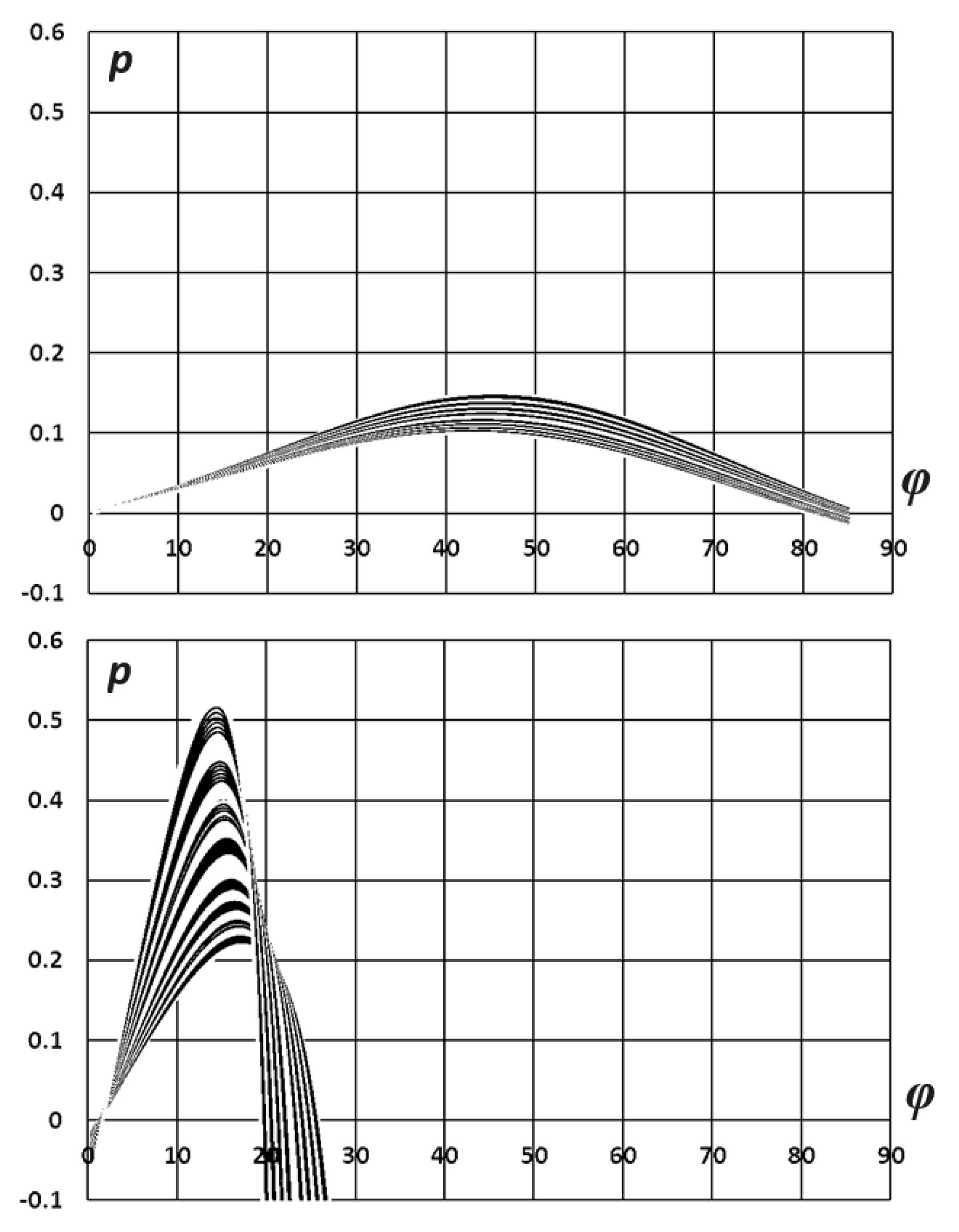
At the same time, with increasing δ, the maxima of p shifts towards lower values of φ. A numerical study of the functions extremums gives the dependence of the optimal value of the blade orientation angle φ on the characteristic angle δ (Figure 15).
If we use the power extracted from the elementary ring as the power scale
then the corresponding power factor (specific power), according to the BEM theory [13] will be determined as
It should be noted that all these calculated characteristics are of a local (differential) nature, that is, they have the meaning of distribution along the turbine blades.
The considered technique can be applied as a numerical experiment for a comparative analysis of turbines with various configurations of rotors and blades, at different driving modes. An analysis of the influence of constructive and regime factors on the energy efficiency of the collinear turbine reveals its modification possibilities to improve dynamic characteristics.
The energy efficiency of collinear turbines. Numerical experiment
The methodology of numerical analysis of the turbine is based on the method of impulse of the blade element BEM. It should be borne in mind that the used version of the BEM does not consider all the components of the emerging flow resistance, so the calculation results are overstated, and energy efficiency indicators are approaching maximum theoretical values. Nevertheless, the model represents a qualitatively adequate picture and makes it possible to evaluate the influence of existing factors [12].
All variables are presented in dimensionless form, in particular, linear quantities (dimensions) are divided by the radius of the turbine. An important characteristic of a turbine is the shape of the blades; they can either widen or narrow from base to tip or have a constant width. In general, you can use the chord function
where is a constant parameter, n is an indicator of the blade shape. It is useful to normalize this function by the total area of the blades, which is determined according to (36)
as an integral (cumulative) function of the area. Integrating from to z=1 gives the total cumulative blade area . Then the normalized function takes the form
In this comparative calculation, three types of blades are considered (Figure 16): linearly expanding (n=1), uniform width (n=0), and tapering in inverse proportion to the distance from the axis (n= -1). When n= -1 formula (57) is transformed into the form
The blade area density index σ is calculated according to (35).
The distribution of optimal characteristic angles δ(z) formed by the relative flow with the turbine axis (with the wind direction) is determined by the family of objective functions (49) presented in Figure 17.
The roots of the equations are determined at the intersections of the curves with the horizontal axis δ. It is possible to use Newton's methods, dichotomy and others. An example of calculating angles δ, as well as optimal blade orientation angles φ, according to (52), is presented in Figure 18.
In addition to δ and φ, the angles of attack ψ distributed along the length of the blade are presented here. They are expressed from δ and φ as
Figure 19 shows the example calculations using the modified BEM method, in the form of the distribution of relative flow velocity vectors and the resultant applied forces to the optimally oriented blade segments.
It is important to keep in mind that there are such aerodynamic regimes when some of the family of equations that describe the aerodynamics at the bases of the blades or, conversely, at their ends, do not have real solutions (roots). The corresponding curves (Figure 17.) do not intersect the δ axis. This means that the calculated extreme power values are not achieved in the corresponding blade sections. In such cases, the values of δ are taken at the maximum points of the curves closest to the δ axis. Typically, these are δ values close to 90°.
Figure 20 shows the distributions along the blades of the coefficients of complex force action on the blades Cx and Cy for a collinear turbine of different speeds.
Substituting the obtained values of angles and coefficients into formulas (46, 47) gives the distribution of the axial and tangential induction coefficients, a and , respectively. Next, local values of the power factor are calculated using the formula (54).
To determine the total integral power factor for the turbine as a whole, the local power in elementary annular sections is recalculated about the swept area of the turbine
where π in the denominator is the swept area of a unit circle (z=1). Corresponding integral power function
At z=1, it acquires the value of the total turbine power factor Cp. The corresponding distributed energy characteristics are presented in Figure 21.
Here the dashed line represents the distribution of the axial induction coefficient a, the double line – the power factor Cp, the thick line – the integral power factor Cpi. The value of Cpi at z=1 represents the power factor of the turbine as a whole. The horizontal dash-dotted lines represent, respectively, the Betz-Zhukovsky limit and the optimal value of the axial induction coefficient corresponding to this limit.
2.3. Compatibility of techniques for collinear turbines
The calculated data from sources [14,15] are compared with the corresponding data calculated using the proposed method. As an example, the original and proposed analysis methods are implemented on a 100 kW horizontal axis wind turbine, model ERDA–NASA MOD-0. The turbine operates at a design rotation speed of 40 rpm, developing rated power at a wind speed of 8 m/s. The rotor has a diameter of 38 meters and has two blades with a NACA 230xx airfoil. Calculations are performed in dimensionless coordinates z=0...1, the number of calculation steps is 20 (see Table 1).
The speed index is calculated using the formula
For the turbine under consideration, it is equal to λ1=9.95.
The distributed data, both source and calculated, are presented in summary Table 2. Table 3 presents the sources used and the corresponding final (calculated) power factor values.
The geometry features of the blade under consideration are such that its initial and final segments (k=1 and k=20) are taken out of consideration to adequately replace the chord function with the dependencies used in the proposed method (see column 5 in Table 2 and Figure 22a).
The main parameter of the inversely proportional chord distribution function is determined by approximation according to the condition of maintaining the blade area
As initial data characterizing the direction of the relative flow, the sources used not the flow angles themselves, but the angles minus the angles of attack (columns 6 and 7 in Table 2), which in the original calculations were constant along the blades and equal 8 degrees (column 11 Table 2). Accordingly, the flow directions are determined by adding columns 6 and 7 with a constant angle of attack (see columns 8 and 9).
For an alternative calculation of relative flow direction angles (column 10), the modified calculation method described above is used. To control the results, it is also useful to calculate the angles of attack of the flow (column 12). The results of calculating characteristic angles are presented in Figure 22b. The applied optimization technique gives values of the relative flow direction angles and distributed angles of attack that differ markedly from their values in traditional calculations.
A comparative analysis of calculation methods shows the following. Although using linear-convex blades implies some increase in flow resistance, optimizing the blade orientation based on maximum power compensates for this. It makes it possible to maintain the high energy performance of the turbine. The comparison of power factors in this example is of limited relevance due to the extremely high-speed index of the turbine. However comparative calculations make it possible to identify other effects, for example, that the energy efficiency of the blade drops sharply near its base, even under conditions of adequate optimization according to the power criterion. It is reasonable to assume that without power optimization, the contribution of these blade sections to the total turbine power is vanishingly small.
When optimizing according to the maximum power criterion, the calculated angles of attack are distributed in a certain way along the length of the blade and can differ significantly from the commonly used values (lines 3 and 4 in Figure 22b). In high-speed turbines they are significantly small and can take negative values. These differences are due to the fact that what is important here is not so much the magnitude of the applied aerodynamic forces as their moments relative to the main axis of the turbine. At the same time, at the periphery of the turbine, the longitudinal resistance to airflow is significantly reduced and, thus, the effect of reduced power at high speeds is partially compensated. Aerodynamic regimes are possible when the peak of the dependence of the power factor on the speed index disappears or moves to the region of higher turbine speeds.
An example of a comparison of source data [15] on the dependence of the turbine power factor (Table 4) on wind speed with the calculated data of the proposed optimization technique is presented in Figure 23.
Figure 23 shows that the values of the power factor according to the modified optimization method are close to the values in the source in the range of 7...12 m/s, but exceed them where the optimal values of angles of attack are greater than usual (in the zone of low wind speeds) or less than them (in the high-speed zone).
2.4. Energy efficiency factors for collinear turbines
Selected results of calculations of energy efficiency of collinear turbines (numerical experiments) in the operating ranges of varying design and operating factors (parameters) are considered.
When comparing collinear turbines with different blade shapes, it can be seen that the highest power, close to the Betz-Joukowski limit, is extracted by a turbine with blades of constant width (Figure 24b). The expansion of the blades (Figure 24c), as well as their narrowing (Figure 24a), results in a decrease in energy efficiency. It is useful to proceed from Zhukovsky’s interpretation, which defines the coefficient of axial induction as the fraction of air in the wind flow that is dissipated, that is, passes by the work disk. It then becomes clear that with expanding blades, the air is dispersed more at the periphery, where the disk resistance is greater due to the high area of the blades. When the blades narrow, on the contrary, the flow is not sufficiently dispersed. Both equally lead to a decrease in power.
This result is somewhat different from traditional BEM calculations, where the best shape is considered to be tapering blades. The reason is that if the twist is not optimized for power, then at the periphery of the blade less power is extracted with greater flow resistance.
The effects of the blade area and their rotational speed on energy efficiency are significantly similar to each other (Figure 25 and Figure 26) and are sometimes difficult to distinguish. Reducing or increasing the area has the same effect as the rotation speed, that is, it leads to a decrease or increase in the induction coefficient, and, in any case, to a decrease in power.
An increase in peripheral speed or blade area leads to an increase in drag and. accordingly, an increase in flow dissipation. First, the growing induction coefficient (Figures 25a and 26a) approaches its optimal value, and the power factor reaches its maximum value (Figures 25b and 26b), Then the growing induction coefficient moves away from the optimum, and the power decreases (Figures 25c and 26c).
One of the most informative and widely used energy characteristics of bladed turbines is the Cp-λ curve (power factor - speed index). An example of such characteristics calculated using the modified BEM method is presented in Figure 27.
The Cp-λ curves contain characteristic maxima, which shift towards lower speed indices with increasing density of filling the working disk section with blades.
The extremes (or inflexions) on this and other graphs (Figure 24, Figure 25 and Figure 26) determine the zones of torque decline that occur when the characteristic angles of the relative flow δ are close to 90°. This can occur both within the framework of the optimization model and under special conditions of loss of real roots of the modified transcendental Maalavi equations in the peripheral zones of the blades. This effect leads to deviations of the calculated values of characteristic parameters from the optimum, which leads to a decrease in the calculated energy efficiency. Since the Maalavi equation is a modified energy (power) conservation equation, the partial disappearance of roots in the family of objective functions g(δ,φ) means that the turbine power, determined based on the rotational characteristics, cannot achieve the useful flow power under any combination of parameters, determined from longitudinal characteristics. This means that optimization is not always achievable, that is, there are local configurations of parameters at which energy dissipation occurs - the transition of part of the energy of an ordered flow into the energy of disordered processes, and ultimately into heat.
The resulting picture of the influence of various factors can become the basis for determining directions and methods for modifying collinear turbines to improve their energy and (or) performance indicators.
3. Configurable optimization of orthogonal turbines
Based on an analysis of literary scientific sources, the problem of optimizing an orthogonal turbine is set, its numerical solution is carried out, and the results obtained are analyzed.
3.1. Orthogonal turbines—Review of sources
Vertical axis wind turbines (VAWT) are inherently simpler in design than horizontal axis machines and lower blade speeds reduce safety and noise concerns. While vertical axis turbines do offer significant operational advantages, their development has been hampered by the difficulty of modelling the associated aerodynamics as well as their rotational kinematics. Article [16] presents the results of a simulation of the baseline VAWT calculated using Star-CCM+, the finite volume method (FVM), and compares them with data obtained from a model with several flow tubes. Limitations of the pipe jet model suggest a low gear ratio because the model cannot reproduce the flow splitting and reattaching cycles that reduce space at high rotation angles. Another limitation is the nonphysical and fragmented nature of the tube flow model. Taking this into account, a simple correction is made to account for the unsteady blade effect. As a result, the BEM model was shown to be able to reproduce the power output of a VAWT unit within 10% when calculating FVM for gear ratios above 2.0. The ease of execution makes the BEM ideal for parameterized studies.
Horizontal axis wind turbines (HAWT) have been widely studied and proven to be technologically feasible. However, wind turbines are moving to new environments, such as floating offshore or in urban environments, where operating conditions vary significantly [17]. Vertical axis wind turbines (VAWTs) may be more suitable and compatible in these conditions. so there is a renewed interest in VAWTs. Although vertical axis wind turbines have a long history, the behaviour of these turbines and their complex flow field are still not fully understood. Insufficient understanding of the complex unsteady aerodynamics of VAWTs and the difficulty of accurately predicting the loads and performance of turbines of this type have led to systematic failures and, as a result, variable interest in VAWTs throughout history. Modern methods of aerodynamic modelling of VAWTs confirm their significant non-stationarity, which plays a decisive role in the aerodynamics of VAWTs. The importance of airfoil design and wake aerodynamics for VAWT is emphasized.
Wind is a free and abundant source of energy, and converting wind energy into electrical energy has no negative impact on the environment. Although energy harvesting using horizontal axis turbines (HAWT) is extremely common throughout the world, the wind speed requirements for electricity generation are relatively high. In contrast, a vertical axis wind turbine (VAWT) can produce electricity at low wind speeds compared to its HAWT counterpart. In addition, VAWT can produce electricity regardless of wind direction, and the installation of VAWT is simple and more economical than HAWT. The aim of the study [18] is to compare the performance of different VAWT models using both numerical and experimental methods and find a model with optimal performance. Standard aerofoil blade designs are considered due to their good aerodynamic characteristics. Graphical design of 2D CAD and CFD modelling (Computational Fluid Dynamics modelling) of five different VAWT models, including three airfoil blades (NACA5510, NACA7510 and NACA9510), was performed using the moving mesh method. Pressure and velocity contours as well as various coefficients such as lift coefficient, drag coefficient, torque coefficient and power coefficient are obtained for all VAWT models. At three different speeds, dynamic moments were experimentally measured for all models.
The half-round model has a higher torque coefficient than both NACA models, with a tip ratio λ of less than 0.32. The power factor generally increases as the tip ratio increases. Torque and power coefficients are usually below λ=0.25; however, once this value is reached, these coefficients increase for most models. Regarding the lift coefficient based on the numerical method, all models except the semicircular model tend to increase concerning λ. It is obvious that airfoil camber affects the overall performance of the VAWT, that is, changing the camber percentage directly affects the drag and lift coefficients, torque coefficient and power coefficient. A new model of the drag force of a two-dimensional flat plate of arbitrary porosity oriented perpendicular to the free flow is presented [19]. Resistance is calculated with energy, momentum and mass conservation limitations. The additional resistance caused by base suction is calculated implicitly using momentum theory, making the model self-contained. The model's predictions show strong agreement with experimental observations over a wide range of porosities, including the solid case, as long as precipitation is absent or suppressed. The proposed models better capture the flow physics and offer improved predictions over the classical Betz model, especially for plates with low porosity. Therefore, applications can be found in wind turbine load and power forecasting using BEM, which largely depends on drag predictions.
Paper [20] presents an improved formulation of the dual multiple flow model (DMST) for flow prediction of vertical axis wind turbines (VAWT). The improvement of the new formulation is that it makes the DMST valid for any induction ratio, that is, for any combination of rotor strength and end speed ratio. This is done by replacing the Rankine-Froude DMST momentum theory, which is invalid for moderate to high induction factors, with a new momentum theory that produces reasonable results for any induction factor and improves DMST predictions, especially as tip ratios increase. This improvement is attributed to the more realistic representation of wake velocities, or equivalently the input velocities into the second rear rotor, from the new momentum theory. The predictions of the two DMST formulations are compared with VAWT power measurements obtained from a high Reynolds number testbed. Despite its simplicity and lack of specific flow physics, the DMST model was found to be reliable in predicting the average power factor VAWT for the range of parameters tested.
Low-order models based on BEM blade element momentum theory demonstrate modelling challenges in predicting vertical axis wind turbine (VAWT) performance compared to computational fluid dynamics, despite the widespread engineering practice of such methods. A study [21] shows that the capabilities of BEM codes applied to VAWT can be significantly improved by introducing a new 3D set of high-order corrections, and demonstrates this by comparing BEM predictions with results in the wind tunnel. Experiments were conducted on three small VAWT models with different rotor designs (H-shaped and Troposkein) and blade profiles (NACA0021 and DU-06-W200).
To bridge the gap between high- and low-fidelity numerical simulation tools for vertical-axis (or cross-flow) turbines, paper [22] developed and validated a drive line model that is a combination of classical vane theory elements and flow models based on Navier-Stokes. Models can be run on coarse meshes while achieving good convergence in terms of average power factor, as well as a computational cost reduction of approximately four orders of magnitude compared to blade-resolution 3D simulations. Submodels for a dynamic stall, end effects, added mass and flow curvature are implemented, resulting in reasonable performance predictions for the high-strength rotor, large discrepancies for the medium-strength rotor, and an overprediction for both cases at high rotor tip ratios.
The ability to self-start is an important feature of wind turbines. Various approaches to describing the self-starting of an H-shaped Darrieus rotor are presented and compared in [23]. The Blade Element Momentum (BEM) approach was compared with 2D and 3D CFD modelling. The BEM model demonstrated the limitations that need to be described to describe bootstrapping behaviour. 2D modelling made it possible to identify non-stationary features of the flow fields and the presence of a complex pattern of vortices interacting with the blade. Additionally, comparisons of 2D and 3D data demonstrated the importance of 3D effects such as secondary flows and tip effects. These effects have been proven to have a positive effect on starting, through an increase in torque. It appears that the launch capabilities of the H-Darrieus are the result of many different factors, which include: blade profile, Reynolds number, secondary flows and three-dimensional aerodynamic effects. The data collected suggests that turbine start-up can occur when the impact of the tip is sufficient to pull the turbine beyond the dead zone. At the same time, they are dissipative for a gear ratio less than 1 and should not be so pronounced as to exclude acceleration of the turbine to a speed close to unity. This delicate balance could explain the conflicting experimental results.
Experiments were conducted on a large laboratory high-strength cross-type turbine [24] to investigate the effect of Reynolds number on performance and wake characteristics and to establish scaling thresholds for physical and numerical modelling of individual devices and arrays. It has been demonstrated that the performance of a cross-flow turbine becomes almost independent of Re at Reynolds number based on rotor diameter ReD≈106 or approximate average Reynolds number based on blade chord length Rec≈2×10⁵. A simple model calculating the peak torque coefficient based on static wing data and cross-flow turbine kinematics was found to be acceptable. Measurements of mean speed and near-wake turbulence showed small differences, in the studied range of Re. The calculated peak torque coefficient exhibits similar sensitivity to Reynolds number as experimental results for a real turbine, making it a better predictor than traditional quantitative estimates of airfoil performance such as lift-to-drag ratio.
Blade element impulse modelling has been successfully applied to evaluate the performance of vertical axis wind turbines. However, their acceptance depends on the availability of an expanded aerodynamic coefficient database. It has been proven that the lack of availability can be overcome by interpolating an existing database for random profile thickness, [25] discuss and validate an extended procedure for generating a database for symmetrical profiles to adopt numerical optimization methods for the design of vertical-axis wind turbines.
Evolutionary algorithms are used to provide optimal configurations for various design purposes. Net performance and annual energy production are considered here to show the capabilities of the numerical code. A corresponding increase in productivity is achieved for all obtained results, showing that numerical optimization can be successfully applied in vertical axis wind turbine design procedures. Despite the attractiveness of CFD and advanced measurement techniques, there is still no complete analysis of the aerodynamic loads on the vertical-axis Darrieus wind turbine blades. Due to the unsteady flow around the rotor blades, blade-wake interactions and the occurrence of dynamic stall, the aerodynamics of this type of wind turbine are very complex. A two-blade rotor was studied numerically for a tip ratio of λ=5.0 [26]. This paper compares results on blade aerodynamic loads obtained using different turbulence models. As a result, quantitative instantaneous blade forces, as well as instantaneous wake profiles behind the rotor, were obtained. The aerodynamic wake behind the rotor is also visualized using dashed lines. All CFD results are compared with experimental data taken from the literature. Good agreement between numerical results and experiment is shown for aerodynamic loads on the blades, as well as for the aerodynamic wake behind the rotor. Blade installation accuracy is a very important factor in determining aerodynamic characteristics. Shifting the blade by 2 millimetres or changing the pitch angle by 1 degree can significantly change the tangential load characteristics.
In all economically developed countries of the world, wind, as an energy source, is beginning to play a significant role in their energy balance. The production and design of efficient wind turbines are continuously expanding. The efficiency of modern wind turbines is determined by the value of the coefficient of wind energy utilization from the unit area of the swept surface of the wind wheel in the airflow. Their design belongs to the category of the most knowledge-intensive production. Work [27] considers a mathematical model of the unsteady operation of a vertical-axis Darrieus wind turbine, which rotates due to the action of the lift force on the wing profile of the working blade. The article presents the developed mathematical formulation of the problem and the method for calculating the angular velocity of the Darrieus wind power device when exposed to an oncoming flow, as well as the obtained results of numerical calculations. According to the calculations carried out according to the developed methodology, reliable results were obtained that well describe the physics of the phenomenon. The developed mathematical model, its numerical implementation and the results obtained can be useful for further improvement of the mathematical description of the problem and when designing the design of vertical-axis wind turbines.
Vertical axis wind turbines (VAWT) are suitable for operation at low wind speeds. The aim of the paper [28] is to develop a low-cost model to evaluate and compare the aerodynamic performance of VAWTs with Gorlov and Darrieus-type straight blades. To this end, a double multistream tube (DMST) model was developed for Darrieus and Gorlov's VAWT. After checking the developed models with the results available in the literature, a comparison was made between the Darrieus and Gorlov VAWTs. The role of geometric and performance parameters on the aerodynamic performance and Gorlov's VAWT torque coefficient curves was then assessed. The performance of the Gorlov rotor was found to be better in terms of efficiency and oscillation.
Straight-bladed Vertical Axis Wind Turbines (SBVAWT) have poor power generation and self-starting ability due to the constant change in blade angle of attack. The study [29] attempts to propose a proper analytical tool for high-strength SBVAWTs because high-strength SBVAWTs can be valuable in application due to their comparatively low operating speed and good self-starting characteristics. To obtain an effective analytical tool to predict and evaluate the performance of high-reliability SBVAWTs, the current DMST model, an analytical method that is widely used to predict and evaluate the performance of SBVAWTs, was evaluated through direct measurements of aerodynamic performance forces on blades. However, the current DMST model cannot provide a good estimate of the aerodynamic forces of high-strength SBVAWTs. To this end, instead of using static aerodynamic force coefficients, the current DMST model uses dynamic aerodynamic force coefficients, which are determined based on experimental results. A new relationship between the angle of attack and dynamic aerodynamic force coefficient was established and applied in the DMST model, resulting in the so-called hybrid DMST model. This hybrid DMST model was verified to have significantly improved accuracy over the current DMST model in estimating aerodynamic force. Although the established relationship between the angle of attack and the dynamic aerodynamic force coefficient may not be universal for high-strength SBVAWTs with different profiles and stiffnesses, the proposed method for obtaining aerodynamic forces applies to any other types of SBVAWTs.
Currently, vertical axis wind turbines (VAWT) are being considered as an alternative to horizontal axis wind turbines in special wind conditions, such as offshore farms. However, complex transient VAWT wake structures have a significant impact on the operation of wind turbines and wind farms. In the study [30], the instantaneous flow fields around and downstream of a VAWT with inclined pitch axes are simulated using an actuator model. The characteristics of unsteady flow around a wind power plant with changing azimuthal angles are discussed. The results show that the total estimated wind energy in the shadow of the wind turbine with a tilt angle of 30° and 150° is 4.0, which is 6% higher than that of a tilt angle of 90°. Thus, suitable placement of wind turbines with different inclination angles can potentially provide greater power output from a wind farm.
The need to increase energy harvesting has led to new ideas and developments to extract more energy from wind. One innovative solution is the use of J-blades for Darrieus vertical axis wind turbines (VAWT), which is based on removing part of the conventional blade on both the discharge and suction sides. Although improved self-starting capabilities of VAWTs have been reported using such blades, only hollow blades having a hair-like structure have been studied in the literature. In [31], six different J-shaped structures are numerically studied. A turbine consisting of blades based on NACA0015 forms the base case and is used to evaluate the 2D numerical models. Blades with a cutout on the outer surface systematically performed better than blades with an inner cutout. The latter exhibited unstable behaviour due to the formation of vortices.
Due to high energy consumption in recent years and global efforts to replace fossil fuels with clean energy, the need for highly efficient renewable energy systems has arisen. Small VAWTs are suitable candidates for clean energy production due to their advantages over other power systems; however, their aerodynamic performance is modest. The paper [32] attempted to improve the performance of Darrieus VAWT by investigating the turbine design parameters using the CFD method. Using the proposed optimized turbine, an economic analysis conducted to estimate the overall net present value showed ideal hybrid power. The assistance of auxiliary blades operating in a wider range of TSR is shown, and the starting power of the turbine is increased by 75.8%. The Kriging optimization model predicted an optimal value of Cp=0.457 that could be achieved using an optimal turbine with N=3, σ=1.2, NACA 0021 profile, AR=0.8 and β=−6°, λ=2.8. Finally, the results of the economic analysis show that a hybrid power system consisting of a VAWT, battery. and converter can be applied to meet the load demand of a site with a lower net present value and energy cost compared to other possible hybrid power sources.
Vertical axis wind turbines (VAWTs) have received increased attention in the off-grid and offshore power generation industries due to their inherent advantages over the more popular horizontal axis wind turbines (HAWTs). These advantages include generator localization, omnidirectionality, and simplified design. However, one of the main disadvantages is lower efficiency, which can be reduced by angling the blades. The use of passively pitching flexible blades [33] can achieve the same results as active pitching without requiring any sensors or actuators and has shown promising results in improving VAWT performance in some cases. Wind tunnel testing was conducted with flexible and rigid NACA 0012 airfoil blades to provide the necessary input data for the Dual Multiple Stream Tube (DMST) model. The results of this study show that a passive conversion VAWT can achieve a maximum power factor that is much higher than that of a rigid blade VAWT. Flexible blades have been shown to perform better at high strength (smaller radius) than rigid blades. In fact, for a 1.0 m radius, the maximum power factor of a rigid VAWT is simulated to be only 10%, compared to 18.9% for a flexible VAWT. This results in an astounding 90% increase in efficiency, VAWTs with flexible blades typically experience less abrupt changes in normal force than those with rigid blades, which may contribute to less fatigue over the life of the turbine. This study is the first attempt in the scientific literature to examine from a design perspective how flexible blades can be used to improve the efficiency or power factor of VAWT.
Discussion of sources: orthogonal turbines
Orthogonal wind turbines are inherently simpler in design than collinear wind turbines. and the reduced rotation speed reduces safety and noise concerns. Although such turbines have significant performance advantages, their development is hampered by the difficulty of modelling the associated aerodynamics and geometry. Insufficient understanding of complex unsteady aerodynamics and the difficulty of accurately predicting the loads and performance of turbines of this type have led to failures in their implementation and, as a result, to periodic declines in interest in orthogonal turbines throughout history.
The ease of execution makes the BEM ideal for parametric studies of orthogonal turbines: flow aerodynamics, blade geometric parameters, optimization based on energy efficiency criteria, and so on. Taking into account the peculiarities of the geometry of orthogonal turbines - double sequential flow crossing the cylindrical working section of the turbine, an adapted BEM model in the form of a double multiple flow model DMST is used to describe the functioning of such turbines.
Despite its simplicity and lack of specific flow physics, the DMST model has proven to be quite reliable. The capabilities of the BEM model can be significantly improved by introducing a three-dimensional set of corrections. Comparisons of 2D and 3D data demonstrate the importance of 3D effects such as secondary flows and blade tip effects. Despite the attractiveness of CFD and advanced measurement techniques, there is still no complete analysis of the aerodynamics of Darrieus wind turbines.
As in collinear turbines, optimising an orthogonal turbine according to the criterion of maximum extracted power is relevant. Comparing the results of such optimization with traditional approaches focused on optimal angles of attack can provide more adequate calculation methods for designing collinear turbines and help overcome problems with their practical application.
3.2. Methodology for optimization of orthogonal turbines
As the basis of the methodology, the double-disk multiple stream-tube (DMST) model is considered, which is a special BEM model adapted for orthogonal turbines, Figure 28 shows a diagram of an orthogonal turbine of unit radius and height h, rotating around the main axis with an angular velocity ω. When rotating, the turbine blades describe a cylindrical working ring, and a cylinder of unit radius represents the base (unit) section of this ring.
The position of any generatrix of the cylinder is characterized by the angular coordinate α (Figure 28b). The cylinder section ABCD orthogonal to the flow and the longitudinal EFGH divide the cylinder into four intersecting zones: the oncoming flow zone (90o<α<270o), the outflow zone (0o<α<90o and 270o<α<360o), the counter flow zone (0o<α <180o), in which the flow and blades move in opposite directions, and, accordingly, a zone of associated flow (180o<α<360o). The orthogonal diametral section ABCD represents the swept section of the turbine.
In the general flow, planes parallel to the main axis of the turbine distinguish an elementary flat flow (Figure 28b) with a width cosαdα (where dα is an elementary increment of the angular coordinate α) and a height h. It is obvious that each elementary flow crosses the cylindrical working section twice, first from the side of the flow inflow zone, and then from its outlet. Accordingly, the application of the impulse method based on the Bernoulli equation involves the consideration of double sequential deformation (dissipation) of the flow, which is the essence of the DMST methodology. Based on the analogy with the collinear model, the total (total) flow dissipation when passing through the working area of an orthogonal turbine is assumed to be equal to 2a, where a is the nominal coefficient of longitudinal induction of the flow. The dissipation of the flow along the trajectory of movement in the working area of the turbine is cumulative, changing from a zero value in the oncoming flow to a value of 2a in the exhaust flow. Figure 29 shows a family of current scattering characteristics - the corrective induction index ξ, determined based on the assumption of linear scattering distribution in the input and output sectors of the cylinder (half-cylinders).
In this case, the parameter of the distribution family is the local induction parameter k, which determines the fraction of flow dissipation in the inlet sector of the cylinder, starting from the free-stream flow ξ=0 to the orthogonal diametrical section 3 of the turbine ξ=2k. At k=0.5 (line 5 in Figure 29), the dissipation of flow is divided equally (symmetrically) between the inlet and outlet sectors of the turbine.
The model of interaction of the airflow with a segment of a linearly convex blade is considered by analogy with the collinear turbine model discussed above (Figure 30). One of the features of the orthogonal model is the use of a coordinate system consisting of radial and tangential axes (Ox and Oy, respectively), rotating together with the blade around the main axis.
According to the above aerodynamic diagram, the relative velocity vector V is determined by its components, radial Vx and revolving Vy. The components are calculated by analogy with the collinear model, with the additional introduction of the local induction coefficient ξa (section 3 on the graph, Figure 29). The frontal and lifting forces of the flow on the blade F1, F2, and F3 are calculated based on formulas (3 - 5). Particular aerodynamic models are formed separately for the incoming and outgoing flows.
Incoming stream
The correction index ξ for the incoming stream (section 3) has a value of 2k. Accordingly, the projection of the nominal flow velocity vector V0 onto the radial coordinate axis Ox
When calculating the revolving component, the projection of the flow velocity onto the rotary (tangential) axis Oy is added to the transfer velocity Ve
Accordingly, the values of the relative flow velocity are determined by the expressions: to calculate the radial components of the applied forces
and for rotary components of forces
Substitution of these expressions into the original formulas of the components of the applied forces (3 - 5), taking into account the calculated values of the squared velocities
gives formulas for applied forces for orthogonal turbines:
to calculate radial components
for rotary components
The sums of the projections of forces on the radial and tangential axes constitute the axial projections of the main vector of applied forces
Entering generalized (effective) coefficients into the description of force action
reduces the expressions for the projections of the main vector to the form
The power extracted from the oncoming elementary flow in the orthogonal section of the working cylinder is equal to the product of the projection of the main vector of forces (in the direction of flow movement) by the speed of the deformed flow in this section
When expanded, the expression takes the form
On the other hand, this same power is defined as the product of the rotational force and the rotational speed of the point of its application on the blade
or, in expanded form,
By analogy with the collinear model, according to the impulse theorem, the longitudinal force is equal to the product of the mass flow rate dm ⁄ dt of the flow and the difference in velocities in the sections of the incoming and outgoing elementary flow ΔVx - Fx=dm⁄dt ΔVx, according to formula (37), and the final expression
Comparison of the resulting expression with formula (80) gives the relation
The rotary relation a'⁄(1+a')=σCy ⁄ 4sinδcosδ coincides with the corresponding relation (43) for collinear turbines.
Comparison of power expressions (83) and (85) gives the relation
Taking into account expressions (43) and (87), this relation is transformed to the form
The value of the induction coefficient in the incoming flow, expressed from (87),
The rotary coefficient of induction a'=(σCy)⁄((4sinδcosδ-σCy)) coincides with the corresponding collinear coefficient (47).
Relationship (89) takes the form
About the method under consideration, relation (91) is transformed into the modified Maalavi equation g(φ,δ)=0, where the objective function
On the other hand, the power expression (85) is transformed to the form
after which a special function is extracted from it
including those components (93) that depend on φ.
Outgoing flow
In the outgoing flow zone, between diametrical section 3 and outgoing flow 5 (Figure 28 and Figure 29), the value of the local induction coefficient ka (in the free flow) is replaced by (1-k)a. Accordingly, the speed in the outlet section of the working cylinder 4 (based on the formation of dispersion on an accrual basis) takes on the value
Relation (88) takes the form
and relation (89)
Relationship (91) takes the form
and is further transformed into the modified Maalavi equation g(φ,δ)=0, where the objective function
The expression for extracted power (93) takes the form
Accordingly, a special function for the outgoing flow
Based on the Maalavi equation and a special function, a system of transcendental equations is formed
similar to system (52) for the collinear model.
The numerical solution of the system gives the optimal values of the angles φ and δ, which characterize the orientation of the blade segments, ensuring maximum extraction of flow power.
First, the parametric family of objective functions p(φ,δ) is examined for the maximum using traditional methods of numerical analysis (Figure 31).
The configuration of the family is such that at large values of the parameter δ, as it increases, there is a slow shift in the maxima of the objective functions towards a decrease in the blade orientation angle φ (Figure 32).
In the parametric zone δ near -90°, the double maxima of the objective functions level off at small and large values of φ, followed by an inversion “jump” of the maximum at a certain critical value of the parameter δ. Further, at a new level of φ values, a gradual shift of the maxima continues towards decreasing the optimal orientation angles φ.
The resulting numerical relation φ(δ) is substituted into the modified Maalavi transcendental equation, and this equation is solved by conventional numerical methods. Figure 33 shows a typical family of objective functions of the Maalavi equation, built according to the angular coordinate parameter α. The roots of the equation δ(α) are located at the points of intersection of the curves with the axis of characteristic flow angles δ.
It should be noted that such combinations (configurations) of design and operating parameters are possible in which some of the curves of the family intersect the δ axis near -90°. or do not intersect it at all, which entails a formal loss of the corresponding real roots. In such cases, the values of δ at the maximum points of the objective functions, as those closest to the δ axis, are used as solutions. Usually, these values are also close to -90o. As applied to orthogonal turbines, such special configuration zones are characterized by a break in the monotonicity of the functions describing the aerodynamics of the turbines. In corresponding graphs and diagrams, these effects are usually reflected in the form of horizontal segments.
Thus, Figure 34 shows the results of calculating, according to the method outlined above, the optimal angular operating characteristics of an orthogonal turbine.
The numerical solution of the system of equations of the form (52) gives the distribution of angles: the direction of the relative flow δ(α) along the circumference of the working cylinder (along the angular coordinate α) and the corresponding blade orientation angle φ(α). In Figure 34 some specific effects are visible. As the speed of the turbine increases, the ranges (amplitudes) of changes in characteristic angles narrow. Angle convergence limits: δ → -90o, ψ → 0o. Near the angular coordinates α=90o and α=270o there are inverse jumps in the orientation angles of the blades φ by an amount of 180o. As the speed of the turbine increases, special configuration parametric zones appear, presented on the graphs in the form of horizontal linear segments.
Similar effects are observed in the distribution of force action coefficients - radial Cx and rotary Cy (Figure 35).
As in collinear turbines, these effects are associated with the loss of roots of the modified Maalavi equations and are physically expressed in dissipative losses of power extracted from the airflow.
The distribution of the induction coefficient along the circumference of the cylinder a(α) is calculated using formulas (47), (90) and (97). Further, according to the basic Betz-Zhukovsky formula, the distribution of the local power factor along the circumference of the working cylindrical section is determined as
It should be borne in mind that Ср(α) characterizes the total energy extraction in a flat elementary flow, both at the entrance to a working cylinder and at the exit from it, that is, for summation (integrating) the extracted powers from elementary flows (preventing double counting of elementary power), for each local elementary power dP(α), reduced to the angular coordinate α, a correction factor of ½ should be entered
where h cosα dα is the area of the orthogonal section of the elementary flow.
The total power extracted by the turbine is determined by integral summation
The operating power factor СрI is the specific flow power divided by the sweeping area of the turbine (the diametrical cross-sectional area of a unit radius cylinder – 2h)
Accordingly, the current integral working coefficient (specific accumulated power), as a function of the angular coordinate
Figure 36 shows an example of a calculation of the distribution of induction and power coefficients and specific integral power.
The final accumulated value of Срi (α=360o) gives the total power factor of the turbine, related to its swept area.
3.3. Effects of blade inversion in orthogonal turbines
A specific property of optimized orthogonal turbines is the effect of blade inversion [34] (Figure 32), occurring both in the counter-flow zone (near the angular coordinate α=90o) and in the unidirectional flow zone (near α=270o). Figure 37 shows the effects of inversion in the form of instantaneous rotation of the blades at angles comparable to 180°, determined from the results of an approximate calculation of the blade configuration based on the modified BEM method.
Inversion of a linearly convex blade occurs abruptly, at the moment when the optimally oriented working plane of the blade becomes parallel to the direction (velocity vector) of the relative oncoming flow. In Figure 38, this moment corresponds to position 0 of the blade, in which the relative velocity is parallel to the flow velocity V0, and the applied force vector Fn0 is perpendicular to this speed and its moment relative to the turbine axis is zero. Immediately before inversion, in position 1, the blade is oriented so that the axial moment of force Fn1 is maximum and directed in the direction of rotation, counterclockwise. In this case, the velocity of the relative flow V1 is directed so that its interaction with the blade occurs from the inside of the working cylinder.
After passing through the inversion point, the velocity of the relative flow V2 changes its direction so that its interaction with the blade moves to the outer side of the cylinder. Accordingly, optimization involves changing the orientation of the blade in such a way that its working plane is on the outside of the cylinder, in such a way as to ensure a maximum of the axial moment of force Fn2, while maintaining its direction.
In the lower part of Figure 38, the blades in positions 1 and 2 are presented combined and reduced (by turning) to a single (zero) inverse position, which makes it possible to identify the reduced (effective) inversion angle Δφ.
It should be recognized that within the framework of the optimization concept of adjustable blades, the use of linearly convex blades is considered exclusively for theoretical analysis since their inversion is practically impossible due to the excessive complexity of implementing turns close to 180°. This effect can be partially compensated by the use of reverse inversion, implemented through the use of symmetrical adjustable blades (Figure 39). With an asymmetric inflow of flow, characterized by an angle ϑ, a symmetrical blade is aerodynamically similar to a linearly convex blade [35] (Rotkin, V.M. 2020) and is capable of producing effects of drag and lift forces (Fn, Fτ) comparable to a linearly convex blade. In this case, the characteristic (maximum) value of the reduced lift coefficient s3 can be considered with acceptable accuracy proportional to the blade opening angle µ.
Given the value s3, the dependence of the current value of the lift coefficient s on the flow asymmetry angle can be described by a piecewise function of the form
In Figure 40, this dependence is represented by composite line 1.
For aerodynamic analysis, simplified approximating piecewise functions can also be used: piecewise linear
(line 2 in Figure 40) and sign function
(line 3 in Figure 40).
The previously discussed methodology for the optimization calculation of orthogonal turbines, with amendments regarding the features of calculating the lift coefficients s3, is quite applicable for turbines with blades of symmetrical cross-section. The main difference from linearly convex blades is (Figure 41) that when the blade is inverted, there is a “jump” from the inner zone of the working cylindrical surface of the turbine to the outer one not only of the centre of contact of the oncoming relative flow with the blade (V1=>V2), but and the working plane of the force action, which determines the directions of the applied aerodynamic forces (Fn1=>Fn2).
Bringing the blades from positions 1 and 2 to a single (zero) inverse position, presented in the lower part of the Figure 41, shows how the direct inversion of the blade Δφ is converted into the reverse inversion of the symmetrical blade in the form of a turn through the angle , usually an order of magnitude smaller than with direct inversion. An example of a comparative calculation of the distribution of blade orientation angles with direct inversion φ and with reverse inversion is presented in Figure 42.
It is useful to note that inversion occurs at critical values of the angle δ, although close to -90o or -270o, but not coinciding with them. Numerical analysis of special functions p(φ,δ) using the BEM method makes it possible to calculate with acceptable accuracy the values of the critical inversion angles , depending on the lift coefficients s3 or the opening angles of the symmetrical blade µ (Figure 43).
Orthogonal turbines with adjustable blades are extremely rare in practical applications. The vast majority of vertical-axis wind turbines use Darrieus rotors - orthogonal turbines with fixed symmetrical blades. At first glance, the possibilities of optimizing influence on such blades are significantly limited, but analysis of the aerodynamic mechanism of fixed blades reveals the possibilities of their self-regulation (Figure 44).
When the blade passes through the critical point (position 0), there is an instantaneous transition of the working plane of the force action, which determines the directions of the applied aerodynamic forces (Fn1=>Fn2), from the internal zone of the working cylindrical surface of the turbine to the external one. Thus, a quasi-inversion of the blade is carried out, in which the inversion angle is equal to the blade opening angle µ. Unlike adjustable blades, this angle is constant, it does not depend on the operating parameters of the turbine and therefore does not provide an absolute optimum in power. However, at certain ratios of opening angles and turbine speed characteristics, quasi-inversion gives power extraction indicators that are close to optimal, and in some circumstances even (paradoxically) exceed them.
Figure 45 presents comparative results of calculations of the distribution of angular characteristics of orthogonal turbines around the circumference of the working cylinders, for a turbine with adjustable blades and a similar turbine with a Darrieus rotor.
The Darrieus rotor is characterized by reduced aerodynamic drag compared to optimized blades, which leads to a decrease in flow dissipation and is manifested in an increase in the amplitude of the optimal characteristic angle δ and, as a consequence, in an increase in the amplitude of the angle of attack ψ (Figure 45b). Since the blades of the Darrieus rotor are fixed, the calculated distribution of the angle of their orientation is conditional - the angle changes sharply from -μ/2 to +μ/2 and characterizes the effect of “jumping” the working plane of a symmetrical blade.
3.4. Compatibility of techniques for orthogonal turbines
The significant (overwhelming) majority of orthogonal vertical-axis wind turbines are low-speed. It is believed that the energy characteristics of such turbines remain at the level of horizontal-axis propeller wind turbines, but the reduction in speed increases the efficiency of orthogonal turbines with a rather simple design of the blade, and the operating range of wind speeds also expands. Accordingly, in well-known experiments, including those aimed at finding means to achieve the maximum possible extraction of wind energy, speed coefficients do not exceed λ=3.
A typical example of experimental verification is presented in Figure 46, where the calculated results obtained for an orthogonal turbine [31] (García A.A. et al. 2021) are compared with the experimental results [36] (Bravo et al. 2007) and the calculated ones [37] ( Daroczy et al. 2015).
Good agreement between the simulation results is obtained, but both numerical results differ significantly from the experimental data, especially concerning the maximum value of 𝐶p and the shape of the curve after reaching the maximum value. Considering the mechanical friction and aerodynamic losses of the struts gives a better agreement between the numerical and experimental results. It has been shown that calculations obtained using 2D modelling tend to overestimate the results.
Since this work involves studying the behaviour of orthogonal turbines in a wider speed range, the calculation results using the author’s modified BEM/DMST model are compared with calculated and experimental data [21] obtained when testing H-shaped orthogonal turbine with a nominal power of 200 W, in the speed range λ=1.3...4.0.
Figure 47 summarizes the comparison between predictions and experiments, showing the agreement regarding power factor Ср. The largest power factor deviation between the experimental and numerical results was at rotational speeds 𝜆 greater than 3.0.
The standard BEM curve (curve 2) tends to overstate power. The combined effects of dynamic stall and flow curvature (curve 3) shift the peak of 𝐶𝑃 towards lower values of λ, which is a peculiar effect caused by flow curvature. Flow curvature can significantly reduce turbine performance, but dynamic flow stall mitigates its harmful effects, leading to deviation of the 𝐶𝑃 curve mainly at high values of λ. The effect of passive torque (curve 4) reduces the entire power curve, especially at low wind speeds, since the drag forces at low wind speeds “weigh” more than at high wind speeds due to the non-linear nature of the passive torque contribution. Activation of all partial models gives curve 5, which includes losses at the tips in 3D, however, the difference between curves 4, 5 and experimental data seems almost insignificant, being within the experimental error.
Given the absence of the above corrections in the modified BEM/DMST model, a comparison of curves 1 and 2 gives a fit similar to collinear turbines. In the range of moderate speeds λ=1.7...3.7. the power factor values are conditionally comparable. For smaller or larger λ, power optimization tends to exceed Cp values relative to traditional BEM models.
3.5. Energy efficiency factors of orthogonal turbines
Selected results of calculations of energy efficiency of orthogonal turbines (numerical experiments) in the working ranges of varying design and operating parameters are considered.
Numerical experiments involve the calculation of distributed indicators of energy efficiency of turbines, presented in the following Figure s: flow induction coefficients a (dashed lines), local power factors Cp (double lines), integral (accumulated) specific power Cpi (solid lines), limit value Cp (limit Betz Срmax – thick horizontal dash-dotted line) and the corresponding optimal value of the induction coefficient aopt (horizontal dash-dotted line).
When comparing orthogonal turbines with different cross-sectional shapes of symmetrical blades, characterized by the opening angle µ, it is clear that within the limits of commonly used values of µ, with increasing opening angle there is a monotonous increase in the power factor Cpi (Figure 48).
This effect is associated with an increase in flow dissipation due to an increase in the aerodynamic drag of the blades. In Figure 48. this looks like an upward shift of the induction curve such that the values of the induction coefficient on average approach the optimal value aopt.
The filling density of the turbine working cylinder by blades, depending on the number of blades and their chord length, has a significant impact on the energy characteristics of the turbine. Figure 49 shows the effect of energy dissipation (loss of roots of the Maalavi equations), expressed in the appearance of horizontal segments in the distribution of induction and power coefficients.
This effect manifests itself already at relatively small specific areas of the blades, and first stabilizes the specific power Cpi, and then significantly reduces it.
Turbine speed is the most important factor influencing its energy efficiency. Increasing speed from λ=2 to 4 gives a significant, almost doubling, increase in specific power - from Срi=0.23 to 0.44, and continues to grow further, up to λ values exceeding 5 (Figure 50).
Then the effect of energy dissipation appears, expressed in the degeneration of the distributed characteristics a and Cp (horizontal segments in Figure 50c). and the stabilization of the integral specific power Cpi, followed by its decline.
An example of a comparative analysis of the energy efficiency of an orthogonal turbine with adjustable blades and a turbine with a Darrieus rotor is presented in Figure 51.
In contrast to fixed Darrieus blades, optimal control of the blade orientation increases the aerodynamic drag of the turbine, manifested in an upward shift in the distribution curve of the induction coefficient a, in comparison with the Darrieus rotor (Figure 51a compared to b). Accordingly, the Darrieus rotor shows, on average, a decrease in the values of the local power factor Cp (relative to the adjustable blades), and as a consequence, a noticeable decrease in the specific integral power Cpi. Thus, in the same parametric configurations, with moderate values of the speed index (λ<6), the Darrieus rotor shows lower energy efficiency than optimized turbines with variable blades (Cp - λ in Figure 52).
However, this does not mean that Darrieus rotors are absolutely inferior in energy efficiency to optimized turbines since the critical extreme values of the speed index of Darrieus rotors are shifted (concerning optimally controlled turbines) towards significantly higher values λ = 10...11, where the maximum power factor exceeds the maximum for the optimized turbine (curve 2, compared with curve 1, in Figure 52).
The calculated results presented above were obtained using several particular examples, however, analysis of an expanded database of numerical experiments makes it possible to make a general qualitative assessment of the influence of some design and operating factors on the energy efficiency characteristics of orthogonal turbines, in terms of their optimization.
Variation of the local induction parameter k during numerical experiments showed that a change in this parameter (that is, the fraction of flow dissipation in the forward sector of the working cylinder - in sections 1-3 in Figure 28) slightly affects the configuration of the ascending branches of the characteristics Ср-λ, however, the maxima of these characteristics reach their greatest values at k=0.35...0.40 and shift towards lower values of λ and Ср when k deviates in any direction from the optimal values.
The optimal design of orthogonal turbines involves the use of symmetrical blades with opening angles in the range µ=12...15 degrees and with a specific blade area (density) Abi=0.05...0.08. An increase in the filling density of the working cylinder blades leads to an increase in the probability of the turbine transitioning into dissipation mode, with a decrease in energy efficiency (a decrease in the Cp parameter).
For turbines with adjustable blades, according to calculation results, the optimal blades are those with parameter values close to the maximum (within the limits recommended above): with opening angles of up to 15° and with a specific area of 0.08. Such turbines are relatively low-speed, providing specific power up to 0.5, with speed indicators at the level of λ=5. It should be borne in mind that adjusting the blades significantly complicates the turbine design and reduces its reliability. In addition, at low speeds, rotational torques increase, which leads to an increase in the material consumption of both the blades and the turbine as a whole. These circumstances limit the feasibility of using turbines with adjustable blades.
For high-speed Darrieus rotors, on the contrary, lightweight blades with an opening angle of 12 degrees and a specific area of 0.05 are optimal. With speed parameters λ greater than 7, such a turbine is capable of showing energy efficiency Cp greater than 0.5. The limitation of such turbines is the strength of the blades under the influence of centrifugal and vibration loads. The development and use of special materials and new, more advanced design solutions are required.
4. Structural optimization of turbines
Based on an analysis of literary scientific sources, an approach to optimizing wind turbines based on their structural (constructive) modification is considered. Optimization calculation methods are presented using examples of multi-rotor wind turbines.
4.1. Structural factors of energy efficiency—Review of sources
To meet the growing demand for high-power wind turbines, the concept of multi-rotor wind turbines has attracted attention as a promising alternative to conventional large-scale single-rotor wind turbines. The study [38] uses eddy flow modelling to compare the wake flow characteristics of a multi-rotor wind turbine with those of a single-rotor turbine. It is found that the wake of a multi-rotor turbine recovers faster over short distances downwind. The recovery rate of multi-rotor turbine wakes increases by increasing the distance between rotors, while the number and direction of rotation of the rotors do not play a significant role in wake recovery.
The results of research in the field of wind energy converters with increased efficiency - two-rotor and shrouded wind turbines [39] are presented. This paper summarizes and discusses numerical studies of URANS FRM concerning various aspects of SWT operation. The presence of a second rotor can reduce the mass flow through the upstream wind turbine, particularly when the downstream rotor is located close to the diffuser inlet. Qualitatively, the distributions practically do not change. A comparison of the obtained results for the angle of attack and calculated aerodynamic forces correlates very well with the 2D reference data. This is an important observation from the point of view of rotor geometry optimization, as it proves that 2D data used, for example, in hybrid models can be successfully used in shrouded and multi-rotor configurations. The authors believe that the observations presented and the conclusions drawn regarding modelling techniques and variable definition/interpretation apply to larger wind turbines.
It is known that the performance improvement of vertical axis wind turbine (VAWT) pairs depends on the direction of the tailwind, the distance between the turbines and the direction of rotation. However, there is a lack of reliable numerical models investigating the influence of these parameters. The study [40] performed 2D CFD modelling of an isolated VAWT, as well as pairs of co- and counter-rotating VAWTs, to determine turbine layouts that can increase the power output of VAWT farms. For the configurations analyzed, pairs of VAWTs demonstrated a 15% increase in power output compared to operation in isolated mode when the second rotor was located three turbine diameters downstream and at an angle of 60° to the wind direction. Moreover, when three turbines were arranged in series, the power output was greater than that of a pair by another 3%. The potential applications of VAWTs are endless because turbines are cheaper, easier to manufacture and easier to maintain. For example, remote villages and islands that rely primarily on electricity from diesel generators, or off the UK coast. The common factor is that a VAWT farm will likely be limited not by the efficiency of the turbines, but by the wind energy available at the site.
Due to the potential of diffuser wind turbines to exceed the Betz–Zhukovsky limit for energy extraction, they have attracted great research interest. Article [41] provides a thorough critique and review of the most important theoretical models developed to analyze the performance and design of this wind concentrator system. Attention is also given to optimization procedures aimed at estimating the maximum power factor achievable by the diffuser wind turbine. None of these procedures are found to be suitable for this duct geometry, although they do offer some utility from a design perspective. Theoretical models prove that a diffuser wind turbine can exceed the Betz limit, but they do not provide any information about the geometry that can satisfy this condition.
Numerous analytical studies of power augmentation systems can be found in the literature to improve the performance of wind turbines by increasing the energy density of the air on the rotor. Work [42] extends the semi-empirical model of a shrouded wind turbine to include a convergent-divergent nozzle system. Increasing mass flow can be achieved through two basic principles: increasing the area ratio and/or decreasing the negative outlet backpressure. Theoretical analysis predicts an ideal thrust coefficient below or above 8/9, depending on the back pressure ratio at which the closed turbine operates.
The power output of a wind turbine depends on the size of its rotor, and wind turbines with larger rotor diameters (>175 m) are currently available on the market. However, the main problems associated with such large conventional turbines are their cost and noise pollution. For this reason, researchers [43] have shifted their attention to equivalent smaller-sized multi-turn wind turbines. The simulation results confirm the suitability of a multi-rotor wind turbine instead of a single-rotor configuration. These turbines provide higher energy output at low installation costs compared to single-rotor turbines.
The performance of counter-rotating wind turbines (CRWT) is highly dependent on the aerodynamic design. In the paper [44], the interaction of threads is considered in a theoretical model based on the theory of the drive disk with wake rotation. This method is applied on 500 W casings for a wind turbine with counter-rotation rotors (CRWT) and a wind turbine with a single rotor (SRWT), with the same radii. Wind tunnel tests were carried out on prototypes, with the rotation speed and pitch of both rotors being controlled independently at different wind speeds. At rated wind speed, the maximum power factors CRWT and SRWT were 0.426 and 0.373. Despite the slightly high initial wind speed, the CRWT demonstrated a higher power factor than a single turbine at wind speeds of 8–14 m/s, with a relative power factor gain of 5.3–28.9%.
An intelligent wind turbine (IWT) has two stages of blades rotating in opposite directions [45,46]. This type of wind turbine has a characteristic that self-adjusts in speed due to the torque difference between the two stages of the wind turbine's horizontal axis, so there is no need for a pitch controller to control the speed and shut down the wind turbine due to high wind speed. The performance of the IWT was simulated using Computational Fluid Dynamic (CFD) software, showing that there is no resistance to counter rotation, each blade should have the same torque output.
Review [47] focuses on large-scale horizontal axis wind turbines. Recent developments in horizontal axis wind turbine noise research are summarized. Significant progress has been made in understanding the generation and propagation of wind turbine noise and the impact of wind farm noise on people, birds and animals. In addition to community concerns about the impact of wind farm noise on people and how best to regulate wind farm noise and verify installed wind farms for compliance, turbine manufacturers have shown significant interest in developing quieter rotors to allow wind farms to be installed closer to populated areas, points.
A questionnaire to respond to noise from wind turbines was administered to 361 subjects living near 8 wind farms [48]. A general health questionnaire assessed the respondents' current mental health status. For the areas where respondents lived, sound pressure levels (SPL - Sound Pressure Levels) were calculated as the sum of the contributions of wind farms in a particular area. Typically, 33.0% of respondents were annoyed by noise from wind turbines outdoors.
Various noise generation mechanisms in wind turbines and possible noise reduction methods are considered [49]. Particular attention is paid to the consideration of sources of aerodynamic noise and recent advances in the field of aerodynamic noise reduction. Several studies on the health effects of wind turbine noise have linked wind turbine noise to irritation and sleep disturbance. Trailing edge noise and influx turbulence noise predominate in the low-frequency region. The tip noise dominates the high-frequency portion of the noise. The shape of the tip controls the strength of the tip vortices and the spacing between them, which affects tip noise. Most of the noise is from the trailing edge since the source is generated from the exiting parts of the blade where the flow velocity is higher. Biomimicry has provided leading edges of teeth and slots to reduce noise from this source. Leading edge slots have been shown to outperform serrated slots and provide very significant noise reduction. Reducing tip noise can be achieved by optimizing the tip shape to reduce swirl forces and reduce swirl interaction with the tip edges.
First-generation wind turbine (WT) blades are now reaching the end of their life, signalling the beginning of a major challenge for the future [50]. Currently, most waste is sent to landfill, which is not an environmentally friendly solution. The environmental impact of a single blade's life cycle is assessed using environmental data for raw materials, manufacturing processes, transportation, and operation and maintenance processes. Based on installed capacity in 2014, the total mass of the blades is 78 thousand tons, their energy consumption is 82 TJ, and their carbon footprint is 4.35 million tons. These Figure s will serve as a basis for proposing possible solutions to reduce the environmental impact of wind turbines.
Wind turbines are typically designed for relatively high wind speeds, typically around 10-15 m/s. At lower wind speeds, commercially available wind energy systems do not produce significant amounts of energy. This either eliminates them from use or results in very inefficient energy extraction in regions with lower wind speeds. With careful turbine and generator design, power generation is significantly superior to commercial turbines at low wind speeds [51]. This will allow the use of wind energy where low wind speeds prevail. This will include power for remote weather telemetry stations, radio broadcasts, rural housing and schools, as well as applications requiring an uninterruptible power supply, such as near oil production, refining, refuelling and transportation sites, and military posts.
The specific technology used when converting wind energy into electricity has a significant impact on the cost and reliability of power generation. To assist in selecting the best transmission technology, paper [52] provides a detailed overview of the three main wind turbine transmissions, namely gearbox, direct drive and hydrostatic. Although the gearbox transmission has offered a mature and applicable technology, some inherent difficulties in the manufacture of specific generators, as well as advances in hydraulic engineering, have led to the emergence of new technologies that are the true competitors of the gearbox. The cost, performance and functionality of these transmissions are now comparable to their transmission counterparts.
A load-based analysis approach has been proposed to predict the service life of wind turbines [53]. Physical models are used to estimate the load profiles at the wind turbine blade root, rotor hub centre, and tower head. The effects of surface roughness, crosswind, yaw, rotor and blade cone, individual blade pitch, and wind turbulence are considered and quantified. It is shown that centrifugal, Euler and Coriolis accelerations predominate in the loads on the base of the blades. The pitch angle as well as the pitch of the individual blades influence the rotor hub and the dynamic loads on the tower head. In addition, the actual wind speed distribution is taken into account, which is also a critical parameter for predicting the service life of the installation.
Discussion of sources: structural factors of energy efficiency
The main problems associated with large turbines are their cost and noise pollution. The concept of multi-rotor wind turbines is a common alternative to conventional large-scale single-rotor turbines. These turbines provide higher energy output at low installation costs compared to single-rotor turbines. Turbines with two stages of blades rotating in opposite directions are also being considered as an implementation of the concept of multi-rotor wind turbines. The transition to multi-rotor turbine designs is accompanied by significant changes in the distribution and variation of rotary speeds of the blades. An assessment of the efficiency of wind energy extraction is required for each increase in the number of blades and changes in their speeds. The higher the number of blades, the lower the minimum flow speed to achieve an effective power factor. In single-rotor turbines, high coefficients are achieved in the range of 1 to 3 blades. In multi-rotor turbines, the optimal distribution of blades, taking into account their number, can differ significantly.
Wind concentration systems are increasingly used in wind energy. Attention is given to optimization procedures aimed at estimating the maximum power factor achievable by a diffuser wind turbine. Energy efficiency in turbines with flow concentrators is achieved at a higher rotary speed.
Considering the significant impact of design modifications on the speed of turbines, the appropriate adaptation of wind generator transmissions is of particular importance. The main transmissions of wind turbines are gearboxes, direct drive and hydrostatic. Although the gearbox transmission has offered reliable technology, some of its inherent shortcomings, as well as advances in hydraulic engineering, have led to the emergence of new technologies that are the true competitors of the gearbox. The cost, performance and functionality of these transmissions are now comparable to their transmission counterparts.
Significant progress has been made in understanding the generation and propagation of wind turbine noise and the impact of wind farm noise on people, birds and animals. Turbine manufacturers are showing significant interest in developing quieter rotors. Particular attention is paid to the consideration of sources of aerodynamic noise and recent advances in the field of aerodynamic noise reduction. It should be noted that the noise level of wind turbines significantly depends on their speed. Therefore, structural modification of turbines, leading to a decrease in their optimal speed characteristics, is essential.
4.2. Uniform power distribution concept
Collinear turbines are capable of achieving high energy efficiency levels close to the Betz-Zhukovsky limit. However, these possibilities are realized at significantly high rotational speeds, which entails the negative consequences described above. Partially, this problem can be compensated by adequate design of turbines based on the modified BEM method with optimization according to the power criterion. However, a radical solution to the problem requires fundamentally new approaches.
The analysis shows that the main source of these problems is predominantly geometric (kinematic) in nature - this is the uneven linear field of peripheral velocities of the turbine rotor (Figure 53a) Ve=ωz, where ω=const is unified (independent of z) rotary velocity. It is the unevenness of the velocity field that creates the conditions when acceptable total (averaged) power is extracted only at high speeds at the periphery of the rotor. If a uniform distribution of speeds is achieved along the radius of the turbine, then it can be assumed that more total power is realized at significantly lower speeds. Figure 53b shows a modification of a collinear turbine, divided into several annular coaxial rotors rotating with angular velocities inversely proportional to their radii ω=Ve/z, where Ve=const is unified (independent of z) rotary velocity. Such movement of the blades, characterized by a uniform velocity field, is called quasi-translational (instantaneous translational) in mechanics, in contrast to ordinary rotational and (or) translational movements.
To implement the proposed concept, it is necessary to redistribute the area of the blades, optimally changing their shape, following the selected value of the peripheral speed, This constitutes a separate task of calculating and comparing conventional and modified turbines.
4.3. Segment-disk aerodynamic model
Blade segments in plan view can have different shapes. For this study, a local blade in the form of a round plate is considered (Figure 54). An indicator of the plate orientation is the angular coordinate - the angle 𝜑 between the flow direction Vo and the normal n to the flat base of the local blade.
Considering that the absolute and portable velocity vectors are mutually perpendicular, the relative speed can be calculated from the expression
Substituting the peripheral speed parameter gives
Since the projection of the relative velocity onto the blade normal n is equal to the difference between the corresponding projections of the absolute and portable velocities
then
and the applied airflow forces are converted to the form
Here
- standard flow force, which is defined as the force of transverse frontal action applied to a stationary plate from the side of normally directed flow,
- specific coefficient of longitudinal resistance,
- specific lift coefficient.
Accordingly, the power of forces applied to the segment
It is more convenient to operate with specific power
the expression for which takes the form
Energy-efficient operation of a wind turbine requires the optimal location of its blades about the airflow. Studying the dependence of p(φ) on the extremum makes it possible to identify the optimal orientation of the blade of a collinear wind turbine, depending on its location on the reference axis. Extremum condition
after differentiation and subsequent transformations it takes the form
To present this relationship explicitly, we consider a triangle formed by the vectors of absolute, relative and portable velocities (Figure 3), from which it follows
If, in addition, we introduce into consideration the angle of “additional optimal rotation” χ, which characterizes the effect of the longitudinal action of the airflow, which is calculated from the dependence
then a comparison of the expressions for tan(2β), tan(δ) and tan(χ) gives the relation
Accordingly, explicit optimal value of the angle φ (Figure 55)
For convenience of calculations, expression (123) is reduced to the form
where
Figure 56 shows some calculation results. All characteristics of “the reduced power - peripheral velocity parameter” are characterized by the presence of maxima (not all are in the field of the Figure 56), the location and value of which depend on the parameters of drag and lift. Thus, both a decrease and an increase in the turbine rotation speed concerning its optimal values lead to a decrease in the extracted power.
Studying the dependences by the conditions of extremum dp⁄dλ=0 gives a cubic
the roots of which determine the coordinates of the maxima (Figure 56).
Comparative energy efficiency calculation
A three-blade turbine with a maximum reduced power in the range of peripheral speed parameter values from 4 to 5 was selected as a base object for a comparative analysis of high-speed and low-speed wind turbines. The selected turbine is represented in Figure 56 and Figure 57 by points N1 and M1. The design layout diagram of this turbine is shown in Figure 58a. Each blade is represented by three local blades located at three levels. The blades of all levels rotate as a single rotor, with the same angular velocities. Their linear speeds (and peripheral speed parameters) are proportional to the radii of the levels.
The calculated values of the corresponding parameters of the peripheral speed and reduced power for the blades at three levels (coordinates of points N1, N2 and N3 in Figure 56) are given in Table 5.
Total reduced power of a three-blade turbine
The layout diagram of a multi-blade three-rotor turbine (Figure 58b) differs from the basic one in the following ways:
peripheral speeds (and corresponding parameters) at all three levels are the same and equal to the smallest value in the base turbine (λ3=1.55);
respectively, the number of local blades is distributed between levels in proportion to their radii (external level - 9; intermediate - 6; internal - 3);
local blades at each level belong to a separate rotor, located on the turbine axis.
Since all 18 local blades move at the same peripheral speeds and produce the same reduced power p3, total reduced power of a low-speed three-rotor turbine
The results of the comparative analysis show, that a conventional three-blade wind turbine can be modified without power loss, into an equal-scale low-speed multi-rotor turbine.
4.4. Continuous aerodynamic model
For comparative purposes, the concept is taken to its logical conclusion by considering a multi-rotor turbine, formed from elementary ring segments. An important characteristic of the modified turbine is the distribution of the area of equivalent blades. The area is redistributed due to the expansion of the blades at the periphery of the turbine, which turns out to be possible due to improved dynamics with a decrease in peripheral velocities.
Such a turbine is characterized by constant (independent of z) values of the speed coefficient λm=const. The comparison is made with a conventional turbine with blade shape index n. A conventional turbine has a linearly distributed speed coefficient
In engineering calculations, a simple empirical approach [13] is used, which establishes the relationship between the speed index λ and the number of turbine blades B
Following this formula, the total chord of the blades is related to the speed index by the relation
applicable for each blade annular section (z-values). When comparing the original and modified turbines, it turns out
whence follows
Thus, the modified turbine has a linearly expanding aggregate chord of blades (Figure 59b).
A numerical experiment using the BEM method shows (Figure 60a,b) that a decrease in the speed index λ1 of a conventional turbine (Figure 60a) to the expected values of a modified multi-rotor turbine - from 6 to 3 units, while maintaining the shape and area of the blades (n; AbI), entails a significant decrease in power factor (Figure 60b), which is associated with a decrease in flow dissipation due to reduced blade resistance.
The subsequent modification of the turbine while maintaining the values of the main parameters leads to a significant increase in the power factor, which reaches values very close (almost equal) to those of the original high-speed turbine. At the same time, despite the decrease in the speed of the blades, their flow resistance on average increases, and the induction coefficient increases, approaching the optimal value (Figure 60c).
It must be borne in mind that in a modified turbine all segments of the blades operate in a single universal mode: at the same orientation angles and uniform distribution of the main parameters.
4.5. Two-rotor low-speed turbine: calculation example
Preliminary calculation of the turbine using the basic method is carried out based on the modified BEM method, using Maalavi's transcendental equations, according to the maximum power criterion.

Table 6.
Basic initial data.
| Name | Designation | Meaning |
|---|---|---|
| Generator speed, rpm. | ν | 600 |
| Blade length, m. | L | 0.2 |
| Large rotor radius, m. | R1 | 0.5 |
| Small rotor radius, m. | R2 | 0.25 |
| Blade speed index | λ | 3 |
| Air density, kg/m3 | ρ | 1.2 |
Turbine layout
The turbine contains two rotors with radii R1=25 cm and R2=50 cm (Figure 61).
The large rotor is fixed on the generator shaft, and its speed is ν2=600 rpm. The small rotor is located on its shaft, coaxial with the generator shaft. It is connected to the large rotor by a 2:1 overdrive transmission, and its velocity is twice as high - ν1=1200 rpm. Recommended number of blades: 3 in a small rotor, 6 in a large one.
Calculation of blade chords
Due to the geometry of the small rotor, the distribution of rotational speeds in its blades differs little from conventional single-rotor turbines. For such turbines, tapered blades are optimal. Calculations using the basic method give an acceptable value for the small rotor power factor
when distributing chords of blade sections
where C1 is the total length of the chords in the sections of the blade, cm, X is the distance from the base of the blade to the current section (Figure 62). The total length is understood as the sum of the chord lengths of all rotor blades (the product of the chord of a single blade by the number of rotor blades N). Accordingly, the chord of the blade is calculated
Cp1=0.426
With a three-bladed small rotor, we obtain the reference values of the chords: at the base of the blade , and at the end - 14 sm.
In a large rotor, the active zone is distributed around the periphery, as in low-speed multi-bladed turbines, so linearly expanding blades are optimal. According to the basic calculation methodology, the best energy efficiency
is achieved when the chords are distributed
Cp2=0.329
Chord of individual blade
With a six-bladed large rotor, we obtain the reference values of the chords: at the base of the blade C2b0=1.41 cm, at the end - C2b2=2.34 cm.
Calculation of twist angles
The calculation of the distribution of twist angles of the sections of these blades along the blades was carried out using the basic method, and the results are presented in Table 7 and Figure 63.
Here φ1, φ2 are the angles of inclination of the rectilinear bases in the sections of the blades located at distances X from the bases of the blades to the plane of rotation of the turbine (twisting angles), for the small and large rotors, respectively. Intermediate values of the angles can be obtained by interpolating the table values.
Blade section shape
The basic shape of the sections (Figure 64) was selected based on the following conditions: the bottom surface is flat to provide adequate drag force F1 at any angle of attack; the upper surface is modified cylindrical (elliptical); the frontal contour on the left is narrowed so that the “aerodynamic chord” does not deviate from the lower plane (base) when the angle of attack changes.
The upper surface in the frontal area is modified in a "crocodile" shape so that F3 ("net" lift) is effective even at small negative angles of attack.
The generatrix of the cylindrical surface is a circular arc turned 60°. The chord formed is equal to the radius of the base circle.
The working coordinates of contour points can be both calculated and defined graphically.
If it is necessary to change the ratio of the longitudinal and transverse frontal sections of the profile, you can vary its height (Figure 65), deforming the profile and defining the corresponding variables (coordinates).
Rated power calculation
The rated power of a two-rotor turbine is calculated by the formula
where Cp is the total (effective) power factor of both turbine rotors; A2 – a swept area of the turbine (equal to the total cross-sectional area of the large rotor); V0 – nominal design speed of airflow (wind).
The total power factor is determined by summing the coefficients of two rotors, taking into account the weighting coefficients (the difference in the swept areas of the rotors)
Cumulative coefficient value
Cp=0.435.
Ометаемая плoщадь турбины
Corresponding value
Taking into account the ratio of rotor speeds ν1=2ν2, the speeds of the ends of the rotor blades are equal
Estimated velocity values
Rated wind velocity
Wind velocity value
.
Rated power of two-rotor turbine
The above example calculation demonstrates the capabilities of the structural optimization technique for collinear turbines based on the concept of uniform power distribution. In addition, this calculation can be used in the design, manufacture and subsequent testing of a small pilot wind power plant.
5. Discussion and Conclusions
The subject of the research is optimization methods for bladed wind turbines. Basic types of turbines are considered - with main axes both collinear and orthogonal to the wind flow, as well as modified turbines - additionally equipped with flow guides and concentrators, multi-rotor, track and others.
Optimization models of the base turbines are based on the BEM blade impulse method, which has proven to be simple but quite reliable.
The significant novelty of the approach to turbine optimization lies in the use of directly extracted flow power as an optimization criterion, rather than angles of attack that give the maximum applied forces, as is usually done in traditional calculations. Such angles of attack usually do not provide maximum torque, much less turbine power.
Optimization problems come down to determining combinations (configurations) of variables and parameters that provide maximum turbine power. In a collinear turbine, the working section is considered in the form of a unit circle, in an orthogonal turbine, it is considered in the form of a cylinder, crossed by stream lines twice: both from the incoming and outgoing flow. Accordingly, the BEM method is adapted to orthogonal turbines, taking into account double intersection, and modified for basic turbines, taking into account changes in the optimization criterion.
Solutions of optimization problems (results of numerical experiments) are presented in the form of distributions of optimal basic characteristics - relative flow direction angles, orientation angles of blade elements, angles of attack, flow induction (dissipation) coefficients, local power factors, and integral specific extracted power. In collinear turbines, the distribution is calculated along the blade, in orthogonal turbines - along the working cylindrical surface, along the angular coordinate. Finally, the results are presented in the form of summary characteristics “turbine power factor - speed index” (Cp-λ). The adequacy of the applied methods is verified by analyzing compatibility with the corresponding calculated results from open sources, which, in turn, are verified by experimental data. At average speed levels typical for certain turbines, the methods show satisfactory compatibility. At low and high speeds, the author's methods, as expected, give higher energy efficiency indicators.
It should be noted that the use of the BEM method without clarifying submodels gives overestimated values of energy indicators, sometimes close to the Betz-Zhukovsky limit, which does not interfere with the comparative analysis of calculation methods, and makes it possible to identify several qualitative effects in the operation of basic turbines. Thus, it has been shown that the extremum of characteristic of the Ср-λ characteristics is apparently associated with the effect of dissipation of flow energy at high turbine speeds.
Calculations show a significant influence of the geometric density of the blades of a collinear turbine (the proportion of blades occupied in the working cross-sectional area of the turbine) on its energy efficiency. Increasing the density of the blades makes it possible to extract significantly more power from the flow at lower speeds, except at extremely high rotational speeds, where a decrease in energy efficiency occurs. For example, with a blade density of 15%, more than 50% of the flow power is extracted at a speed λ=6, whereas with a density of 5%, this effect is achieved only at λ=9. The use of high-speed collinear turbines is driven not by considerations of energy efficiency, but by the desire to lighten structures.
A distinctive feature of optimized orthogonal turbines is the effect of blade inversion in positions where the rotational speeds of the blades are collinear with the wind flow speed. In these positions, there is an instantaneous transition of the interaction of the relative flow with the surface of the blade facing the inside of the working cylinder to the outer surface or a reverse transition. When using adjustable blades with a linear-convex cross-section, optimization requires instantaneous rotation of the blades through inversion angles comparable to 180 degrees. Such practically unacceptable designs can be improved by the use of adjustable blades of symmetrical cross-section, in which, due to the possibility of interaction of the relative flow with both sides of the blade, reverse inversion becomes possible at a relatively small angle, complementing the forward inversion angle up to 180 degrees. And, finally, in the used mainly in Darrieus rotors, fixed symmetrical blades operate in a self-regulating mode, due to the non-parallelism of the outer and inner sides of the blades. In this case, at the nodes of collinearity of the blade and flow velocities, a quasi-inversion effect occurs - an instantaneous transition of the flow influence from the inner surface of the blade to the outer surface (or reverse transition), with an inversion angle equal to the blade opening angle.
For orthogonal turbines with adjustable blades, blades with a geometric blade density of 8...10% are optimal. Such turbines are relatively low-speed, providing power extraction of up to 50% of the flow power, with speed indicators at the level of λ=5. Adjusting the blades significantly complicates the turbine design, reduces its reliability and leads to an increase in material consumption. For high-speed Darrieus rotors, on the contrary, lightweight blades with a specific area within 5% are optimal. With speed parameters λ>7, such a turbine is capable of showing energy efficiency of more than 50%. The limitation for such turbines is the strength of the blades under the influence of centrifugal and vibration loads. The development and use of special materials and new, more advanced design solutions are required.
Structural optimization is implemented through the selection of basic and modified turbine designs with the best energy efficiency indicators, taking into account specific production and operating conditions. Such optimization is considered by comparing a basic collinear turbine with a turbine modified based on the concept of uniformly distributed power. Aerodynamic and energy analysis of collinear wind turbines based on the modified BEM method shows the main reason for their forced speed - the kinematic unevenness of the blade rotation speed field. The large speed of turbines is accompanied by manifestations of dynamic instability, which entails a decrease in reliability, noise pollution of the environment and other negative consequences. Reducing speed while maintaining energy efficiency is an important goal of wind energy. The concept of uniform power distribution is one of the methods for solving this urgent problem. It is implemented through the division of a conventional turbine into a set of coaxial rotors moving at the same rotational velocities. Comparative calculations show that such modified turbines provide energy efficiency close to conventional turbines, with comparable blade areas, but with a velocity reduced by 40...50%.
The concept of uniform power distribution and the corresponding calculation methodology are the basis for the subsequent development and testing of a pilot multi-rotor, low-speed and energy-efficient wind turbine.
Funding
This research received no external funding.
Institutional Review Board Statement
Not applicable.
Informed Consent Statement
Not applicable.
Data Availability Statement
The data presented in this study are available upon request from the author. The data is not publicly available due to the absence of the need to create databases, due to the automatic generation (imitation) of data upon request.
Acknowledgments
The author is grateful to Yu.B.Sokolovsky (candidate of technical sciences, Independent Researcher, Haifa, Israel) and N. Karthikeyan (PhD, Research Scientist, National Institute of Technology, Tiruchirappalli, India) for support and for providing research materials.
Conflicts of Interest
The author declare no conflict of interest.
References
- TouchWind (2023). Generating more energy. Always generating. Any storm. https://touchwind.org/.
- World Wide Wind (2023). Counter-rotating vertical turbines. https://worldwidewind.no/pages/technology.
- Airloom Energy (2023). Utility-Scale Wind Energy at Extremely Low Cost. https://airloomenergy.com.
- Okulov, V.L.; Sorensen, J.N. (2008). Ideal'naya vetryanaya turbina s konechnym chislom lopastey [An ideal wind turbine with a finite number of blades]. Proceedings of the Academy of Sciences, Vol. 420, no. 4, p. 478-483. https://www.researchgate.net/profile/Valery- Okulov/publication/226242189_An_ideal_wind_turbine_with_a_finite_number_of_blades/links/5548b2d4 0cf2e2031b38ae5f/An-ideal-wind-turbine-with-a-finite-number-of-blades.pdf.
- Sokolovsky, Yu.B.; Rotkin, V.M.; Limonov, L.G.; Zyryanov, V.M. 2021) Aktual'naya vetroenergetika. Generatsiya i nakopleniye energii. [Up-to-date wind power engineering. Generation and storage of energy]. Monograph, Novosibirsk: Publishing house NSTU 211с. https://www.researchgate.net/publication/353072895_Up-todate_ wind_power_engineering_Generation_and_storage_of_energy_Aktualnaa_vetroenergetika_Genera cia_i_nakoplenie_energii. 3530. [Google Scholar]
- Karthikeyan, N; Kalidasa, M.K; Arun, K.S; Rajakumarb, S. (2015). Review of aerodynamic developments on small horizontal axis wind turbine blade. Elsevier, Renewable and Sustainable Energy Reviews, Volume 42, pages 801-822. [CrossRef]
- Phengpom, T.; Kamada, Y.; Maeda, T.; Murata, J.; Nishimura, S.; Matsuno, T. (2015). Experimental investigation of the three-dimensional flow field in the vicinity of a rotating blade. Journal of Fluid Science and Technology 10(2): JFST0013-JFST0013. [CrossRef]
- Predescu, M; Bejinariu, A; Mitroi, O; Nedelcu, A. (2009). Influence of the Number of Blades on the Mechanical Power Curve of Wind Turbines, European Association for the Development of Renewable Energies, Environment and Power quality, International Conference on Renewable Energies and Power Quality (ICREPQ’09). [CrossRef]
- Çetin, N. S.; Yurdusev, M. A.; Ata, R.; Özdamar, A. (2005). Assessment of Optimum Tip Speed Ratio of Wind Turbines. Math. Comput. Appl. 10, no. 1: 147-154. [CrossRef]
- Mühle, F.; Adaramola, M.S. and Sretran, L. (2016). The effect of the number of blades on wind turbine wake - a comparison between 2-and 3-bladed rotors. Journal of Physics: Conference Series, Volume 753, Issue 3, p.10. [CrossRef]
- Schubel, P.J; Crossley, R.J. (2012). Wind Turbine Blade Design Review. Wind engineering, volume 36, No. 4, 365-388. [CrossRef]
- Lanzafame, R.; Messina, M. (2007) Fluid dynamics wind turbine design: Critical analysis, optimization and application of BEM theory. Renewable Energy, Volume 32, Issue 14, Pages 2291-2305. [CrossRef]
- Gorodov, R.V. (2009) Netraditsionnyye i vozobnovlyayemyye istochniki energii: uchebnoye posobiye. [Non-traditional and renewable energy sources: textbook] / R.V. Gorodov, V.E. Gubin, A.S. Matveev, - 1st ed. - Tomsk: Tomsk Polytechnic University Publishing House, 2009, - 294 p. ISBN 5-98298-429-9 https://www.studmed.ru/view/gorodov-rv-gubin-ve-matveev-as-netradicionnye-i-vozobnovlyaemyeistochniki- energii_f7a7cb800af.html.
- Maalawi, K.Y.; Badawy, M.T.S. (2001) A direct method for evaluating performance of horizontal axis wind turbines. Renewable and Sustainable Energy Reviews, Volume 5, Issue 2, Pages 175-190. [CrossRef]
- Wilson, R.E; Lissaman, P.B.S; Walker, S.N. (1976).Aerodynamic performance of wind turbines. Report No. NSF/RA-760228, NTIS, Chapters I–III, Oregon State Univ. [CrossRef]
- Kozak, P.; Vallverdú, D. & Rempfer, D. (2016). Modeling Vertical-Axis Wind-Turbine Performance: Blade- Element Method Versus Finite Volume Approach. Journal of Propulsion and Power, 32, 592-601. [CrossRef]
- De Tavernier, D.; Ferreira, C.; Goude, A. (2022). Vertical-Axis Wind Turbine Aerodynamics. In: Stoevesandt, B.. Schepers, G.. Fuglsang, P.. Sun. Y. (eds) Handbook of Wind Energy Aerodynamics, Springer, Cham. [CrossRef]
- Rahman, M.; Ahmed, M.; Bashar, M.; Mitra, A. and Salyers, T. (2017) Numerical and Experimental Investigations on Vertical Axis Wind Turbines of Different Models. Open Access Library Journal, 4, 1-37. [CrossRef] [PubMed]
- Steiros, K. & Hultmark, M. (2018). Drag on flat plates of arbitrary porosity. Journal of Fluid Mechanics, 853, R3. [CrossRef]
- Ayati, A. A.; Steiros, K.; Miller, M.A.; Duvvuri, S. and Hultmark, M. (2019). A double-multiple streamtube model for vertical axis wind turbines of arbitrary rotor loading. Wind Energ, Sci., 4, 653–662. [CrossRef]
- Sanvito, A.G.; Dossena, V. and Persico, G. (2020). Formulation, Validation, and Application of a Novel 3D BEM Tool for Vertical Axis Wind Turbines of General Shape and Size, Applied Sciences, 11(13), 5874. [CrossRef]
- Bachant, P.; Goude, A. & Wosnik, M. (2016). Actuator line modeling of vertical-axis turbines. ArXiv. /abs/1605.01449. [CrossRef]
- Rossetti, A. . & Pavesi, G. (2013). Comparison of different numerical approaches to the study of the H-Darrieus turbines start-up. Renewable Energy, 50, 7-19. [CrossRef]
- Bachant, P. & Wosnik, M. (2016). Effects of Reynolds Number on the Energy Conversion and Near-Wake Dynamics of a High Solidity Vertical-Axis Cross-Flow Turbine. Energies, 9(2), 73. [CrossRef]
- Bedon, G.; Raciti Castelli, M. & Benini, E. (2013). Optimization of a Darrieus vertical-axis wind turbine using blade element – momentum theory and evolutionary algorithm. Renewable Energy, 59, 184-192. [CrossRef]
- Rogowski, K.; Hansen, M. O. L. & Lichota, P. (2018). 2-D CFD Computations of the Two-Bladed Darrieus-Type Wind Turbine. Journal of Applied Fluid Mechanics, 11(4), 835-845. [CrossRef]
- Manatbaev, R.K.; Tulepbergenov, A.K.; Sandybaev, E.E.; Kalasov, N.B.; Bergalieva, S.A.; Otegenov, D.S. (2014). Issledovaniye nestatsionarnykh dinamicheskikh kharakteristik vetroturbiny Dar'ye [Study of non-stationary dynamic characteristics of the Daria wind turbine]. “Izvestia of the National Academy of Sciences of the Republic of Kazakhstan. Physics and mathematics series" ISSN 1991-346X, 2 (294) с. 201-206. https://portal.issn.org/resource/ISSN/1991-346X http://rmebrk.kz/journals/334/fizmat% 28.
- Moghimi, M. & Motawej, H. (2020). Developed DMST model for performance analysis and parametric evaluation of Gorlov vertical axis wind turbines. Sustainable Energy Technologies and Assessments, 37, 100616. [CrossRef]
- Peng, Y. X.; Xu, Y. L. & Zhan, S. (2019). Hybrid DMST model for high-solidity straight-bladed VAWTs. Energy Procedia, 158, 376-381. [CrossRef]
- Guo, J. & Lei, L. (2019). Flow Characteristics of a Straight-Bladed Vertical Axis Wind Turbine with Inclined Pitch Axes. Energies, 13(23), 6281. [CrossRef]
- García, A.A.; Santoso, R. E.; Mohan, H.; Rathore, S. S.; Chakraborty, D. & Verdin, P.G. (2021). CFD-Based J-Shaped Blade Design Improvement for Vertical Axis Wind Turbines, Sustainability, 14(22). 15343. [CrossRef]
- Asadbeigi, M.; Ghafoorian, F.; Mehrpooya, M.; Chegini, S. & Jarrahian, A. (2022). A 3D Study of the Darrieus Wind Turbine with Auxiliary Blades and Economic Analysis Based on an Optimal Design from a Parametric Investigation, Sustainability, 15(5), 4684. [CrossRef]
- Roy, L.; Kincaid, K.; Mahmud, R. & MacPhee, D.W. (2021). Double-Multiple Streamtube Analysis of a Flexible Vertical Axis Wind Turbine. Fluids, 6(3), 118. [CrossRef]
- Sokolovsky, Yu.; Rotkin, V. (2017). The theoretical and technical basis for the optimization of wind power plants. Lulu Press Inc, 112 p. https://www.researchgate.net/publication/341786692_THEORETICAL_AND_TECHNICAL_BASIS_FOR_ THE_OPTIMIZATION_OF_WIND_ENERGY_PLANTS. 3417. [Google Scholar]
- Rotkin, V.M.; Sokolovsky, Yu.B.; Azhmukhamedov, I.M. (2020) Rotor Dar'ye i optimizirovannyye vetroturbiny: sravnitel'nyy analiz [Darrieus rotor and optimized wind turbines: a comparative analysis]. Caspian Journal: Management and High Technologies, No. 1 (49), Astrakhan, Astrakhan State University Publishing House, 111-121. https://www.researchgate.net/publication/341931215_Darier_rotor_and_optimized_wind_turbines_comp arative_analysis_Rotor_Dare_i_optimizirovannye_vetranye_turbiny_sravnitelnyj_analiz. 3419. [Google Scholar]
- Bravo, R.; Tullis, S.; Ziada, S. (2007) Performance testing of a small vertical-axis wind turbine. In Proceedings of the 21st Canadian Congress of Applied Mechanics. Toronto, ON, Canada, 3–7 June 2007; pp. 3–7. https://www.researchgate.net/publication/265987114_Performance_Testing_of_a_Small_Vertical- Axis_Wind_Turbine.
- Daróczy, L.; Janiga, G.; Petrasch, K.; Webner, M.; Thévenin, D. (2015) Comparative analysis of turbulence models for the aerodynamic simulation of H-Darrieus rotors. Energy 90, 680–690. [CrossRef]
- Bastankhah, M. and Abkar, M. (2019). Multirotor wind turbine wakes. Physics of Fluids 31, 085106. [CrossRef]
- Lipian, M.; Dobrev, I.; Massouh, F.; Jozwik, K. (2020). Small wind turbine augmentation: Numerical investigations of shrouded- and twin-rotor wind turbines. Elsevier, Energy, Volume 201, 117588. [CrossRef]
- Hansen, C. and Hansen, K. (2020). Recent Advances in Wind Turbine Noise Research. Acoustics 2020, 2(1). 171-206. [CrossRef]
- Bontempo, R; Manna, M. (2020). Diffuser augmented wind turbines: Review and assessment of theoretical models. Applied Energy, Volume 280, 115867, ISSN 0306-2619. [CrossRef]
- Khamlaj, T.A.; Rumpfkeil, M.P. (2017). Theoretical Analysis of Shrouded Horizontal Axis Wind Turbines. Energies, 10, 38. [CrossRef]
- Sandhu, N. S. & Chanana, S. (2018). Performance and Economic Analysis of Multi-Rotor Wind Turbine. EMITTER International Journal of Engineering Technology, 6(2), 289-316. [CrossRef]
- Zhao, Xu; Zhou, P.; Liang, X.; Gao, S. (2020). The aerodynamic coupling design and wind tunnel test of contra-rotating wind turbines. Elsevier, Renewable Energy, Volume 146, 20, Pages 1-8. 20 February. [CrossRef]
- Sutikno, P.; Deny, B. S. (2011). Design and Blade Optimization of Contra Rotation Double Rotor Wind Turbine. International Journal of Mechanical & Mechatronics Engineering IJMME-IJENS Vol: 11 No: 01 17, 115301-7474. https://www.researchgate.net/publication/228900747_Design_and_Blade_Optimization_of_Contra_Rotati on_Double_Rotor_Wind_Turbine. 2289. [Google Scholar]
- Muisab, A.; Sutiknoa, P.; Soewonoa, A.; Hartono, F. . (2015). Design Optimization of Axial Hydraulic Turbine for Very Low Head Application. Energy Procedia, Volume 68, 15, Pages 263-273. 20 April. [CrossRef]
- Hansen, J.T.; Mahak, M.; Tzanakis, I. (2021). Numerical modelling and optimization of vertical axis wind turbine pairs: A scale up approach. Вoзoбнoвляемая энергия, 171, 1371-1381. [CrossRef]
- Pawlaczyk-Łuszczyńska, M.; Dudarewicz, A.; Zaborowski, K.; Zamojska-Daniszewska, M.; Waszkowska, M. (2014). Annoyance Related to Wind Turbine Noise. ARCHIVES OF ACOUSTICS, Vol. 39, No. 1, pp. 89–102. [CrossRef]
- Deshmukha, S.; Sourodeep, B.; Anuj, J.A.; Ranjan, P. (2018). Wind turbine noise and its mitigation techniques: A review. Part of special issue: 2nd International Conference on Energy and Power, ICEP2018, Sydney, Australia. [CrossRef]
- Barlow, P. L. and Barlow, C. Y. (2016). The environmental impact of wind turbine blades. Published under licence by IOP Publishing Ltd. IOP Conference Series: Materials Science and Engineering, Volume 139, 37th Risø International Symposium on Materials Science, Risø, Denmark. [CrossRef]
- Gitano-Briggs, H. (2012). Low Speed Wind Turbine Design. Open access peer-reviewed chapter. [CrossRef]
- Taherian-Fard, E; Sahebi, R; Niknam, T; Izadian, A. and Shasadeghi, M. (2020). Wind Turbine Drivetrain Technologies. In IEEE Transactions on Industry Applications. vol. 56, no. 2, pp. 1729-1741. [CrossRef]
- Rommel, D.P; Maio, D.Di; Tinga, T. (2020). Calculating wind turbine component loads for improved life prediction. Elsevier, Renewable Energy, Volume 146, Pages 223-241. [CrossRef]
Figure 1.
Wind installations with collinear turbines.
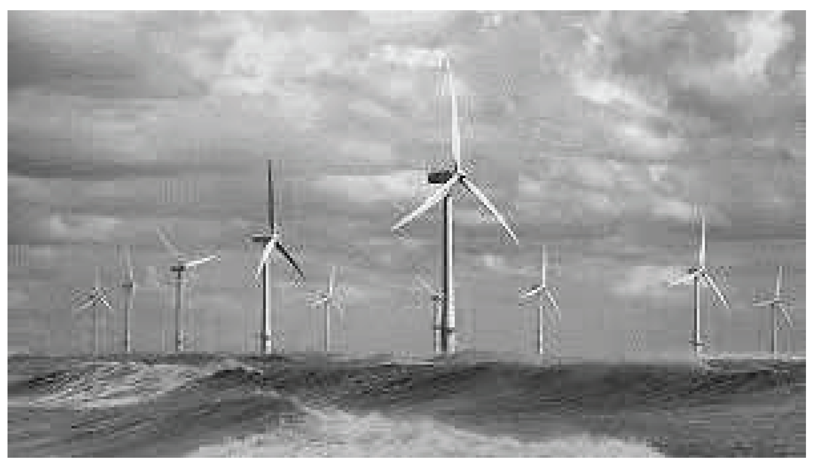
Figure 2.
Schemes of collinear wind turbines: 1 - single-blade with counterweight, 2, 3, 4 - two-, three-, multi-blade.
Figure 2.
Schemes of collinear wind turbines: 1 - single-blade with counterweight, 2, 3, 4 - two-, three-, multi-blade.
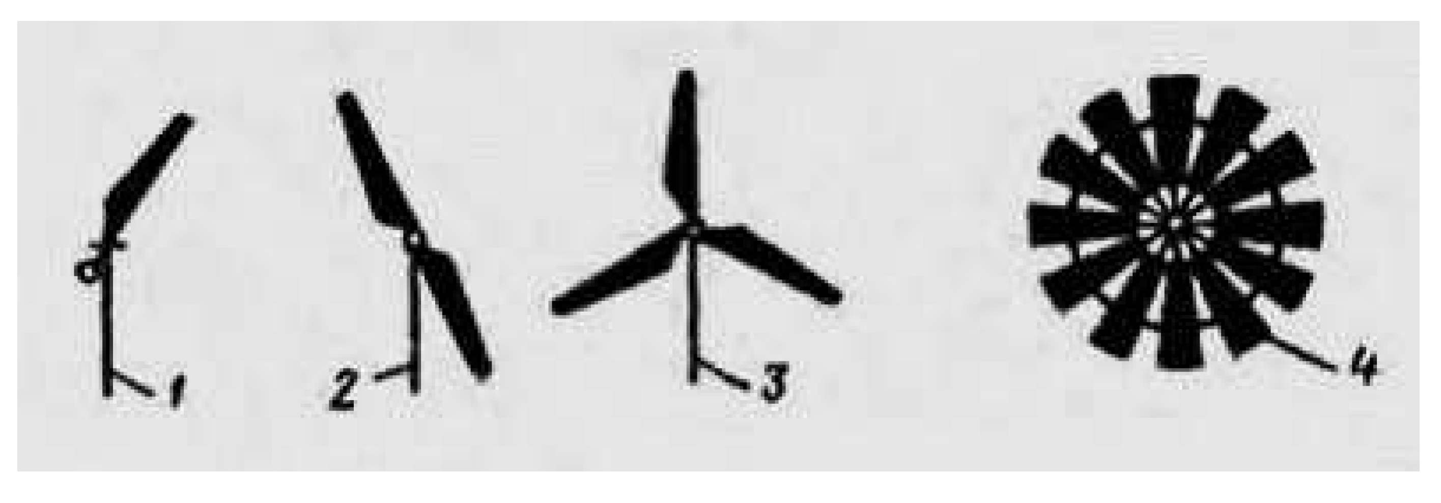
Figure 3.
Wind installations with orthogonal turbines.
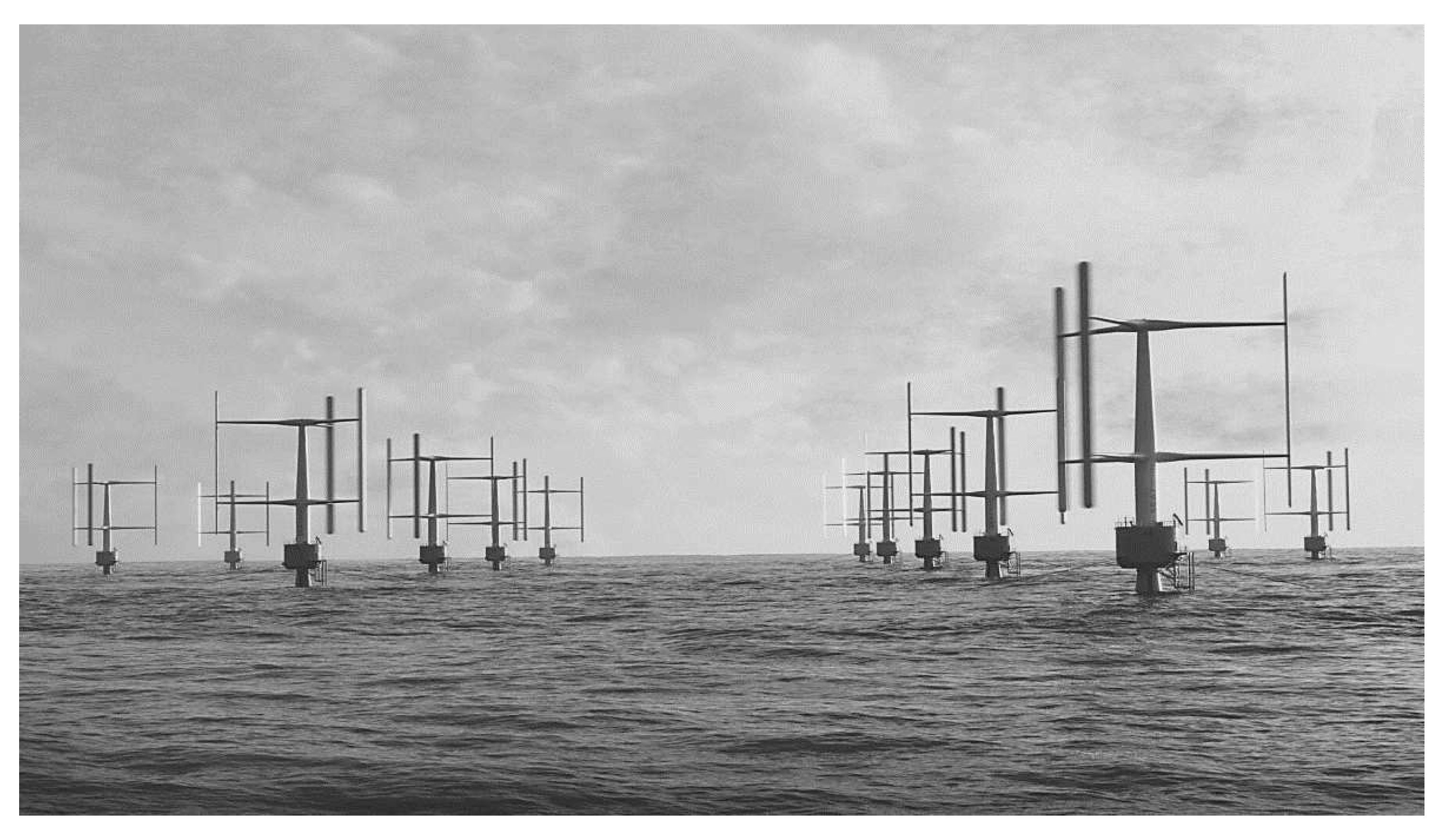
Figure 4.
Schemes of orthogonal wind turbines Darrieus: 1 – H-shaped, 2 – inclined, 3 – curved, 4 – helicoidal.
Figure 4.
Schemes of orthogonal wind turbines Darrieus: 1 – H-shaped, 2 – inclined, 3 – curved, 4 – helicoidal.
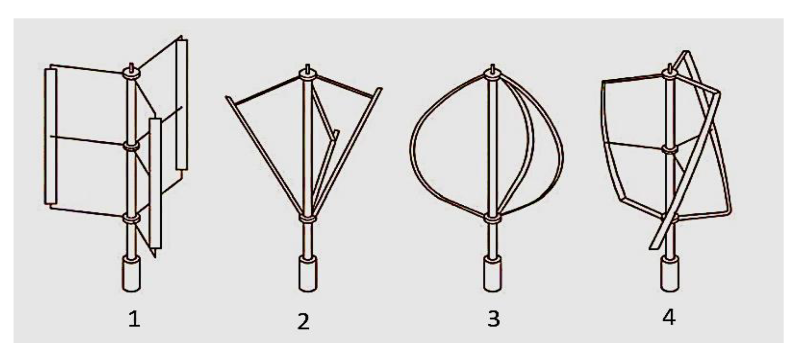
Figure 5.
Multi-rotor collinear wind turbines: on the left is a parallel rotor configuration, on the right is a serial configuration.
Figure 5.
Multi-rotor collinear wind turbines: on the left is a parallel rotor configuration, on the right is a serial configuration.
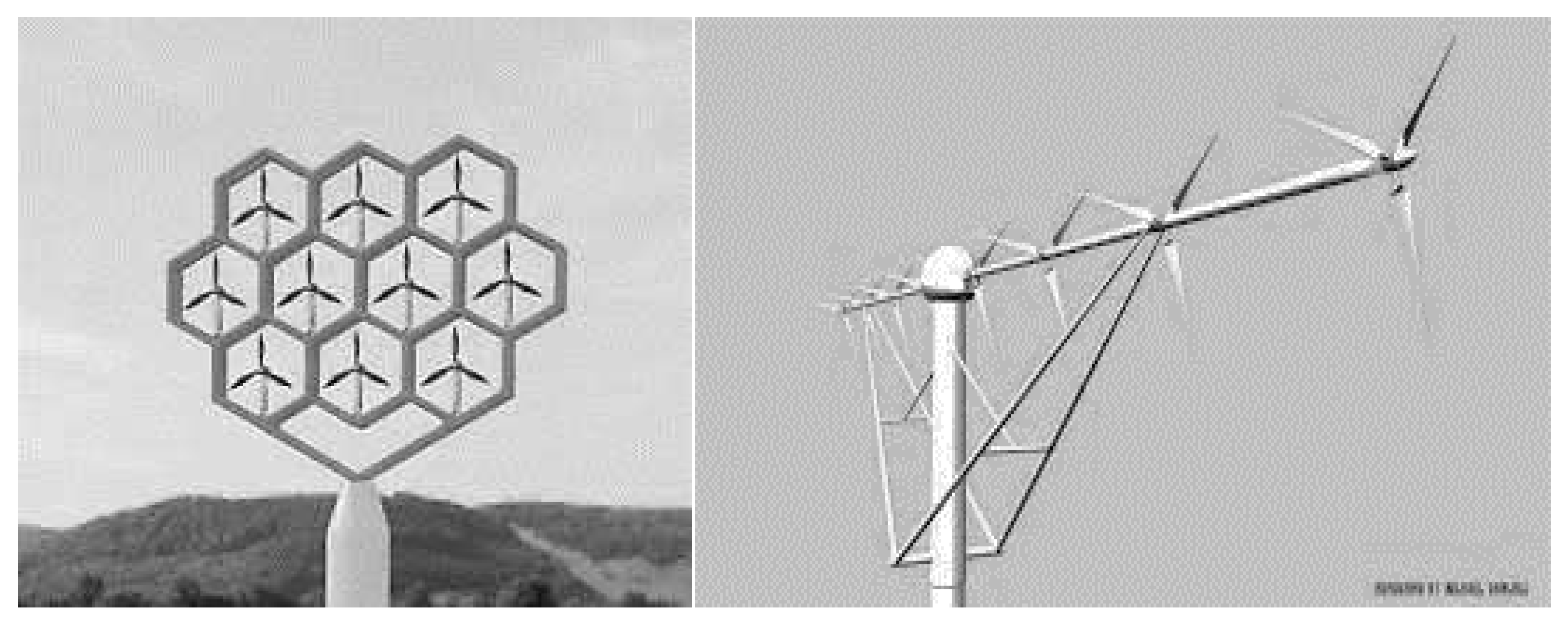
Figure 6.
Diagram of an orthogonal counter-rotor turbine.
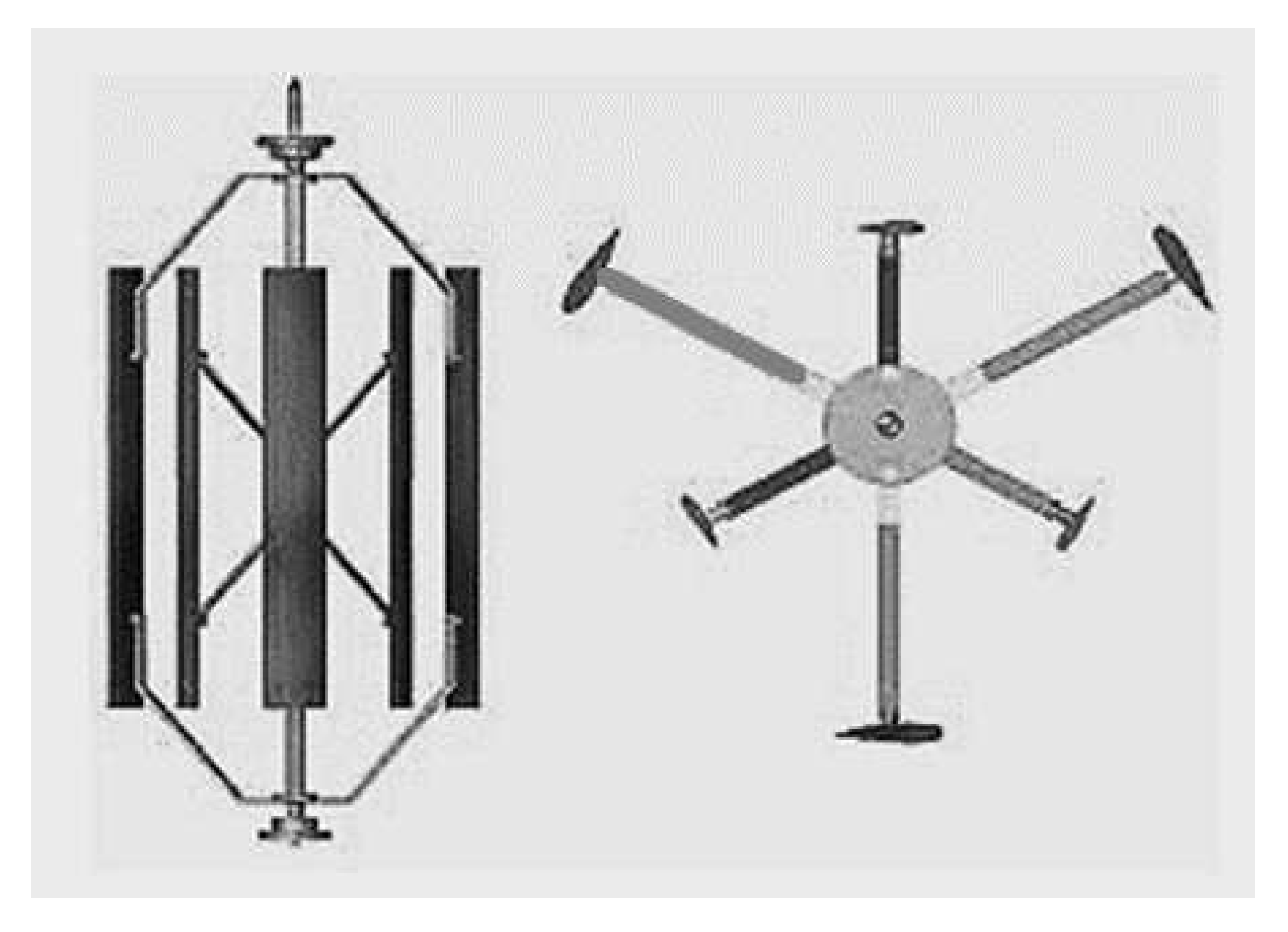
Figure 7.
Collinear turbine with wind concentrator.
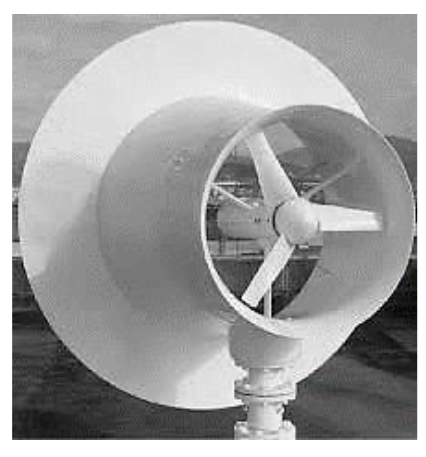
Figure 8.
Innovative adaptive floating turbines: on the left is a turbine with a solid inclined rotor [1]; on the right – counter-rotation turbine [2].
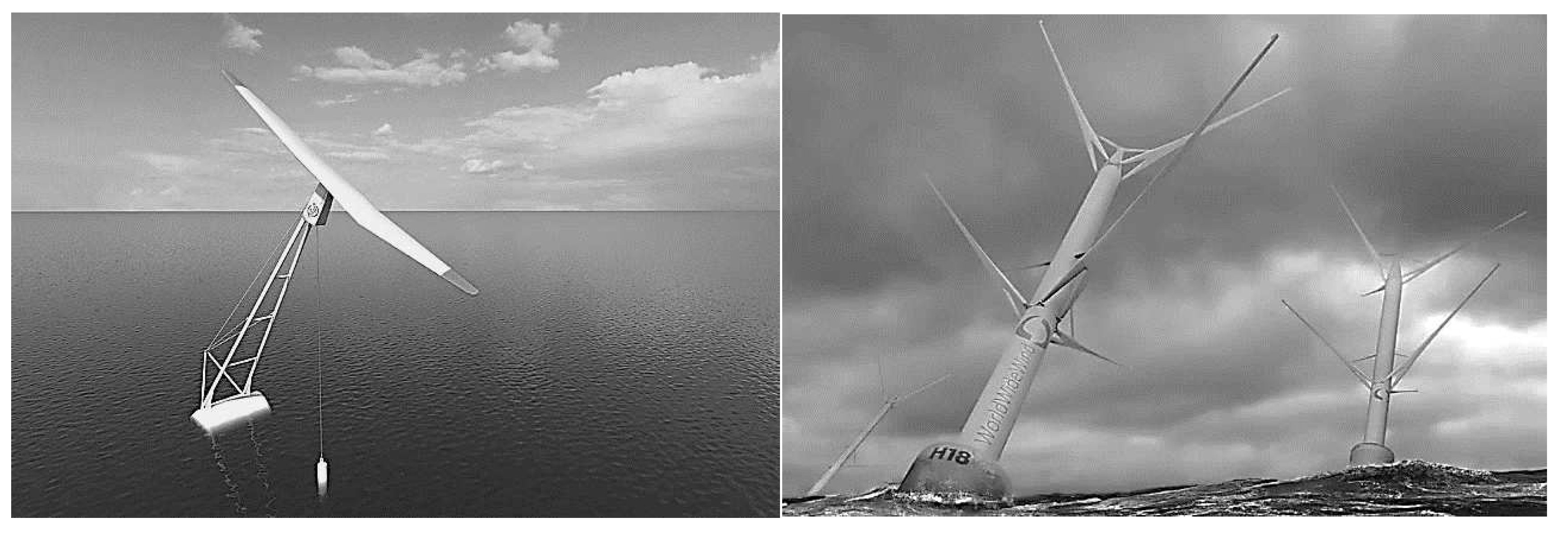
Figure 9.
Innovative track wind turbine 2.5 MW [3].
Figure 9.
Innovative track wind turbine 2.5 MW [3].
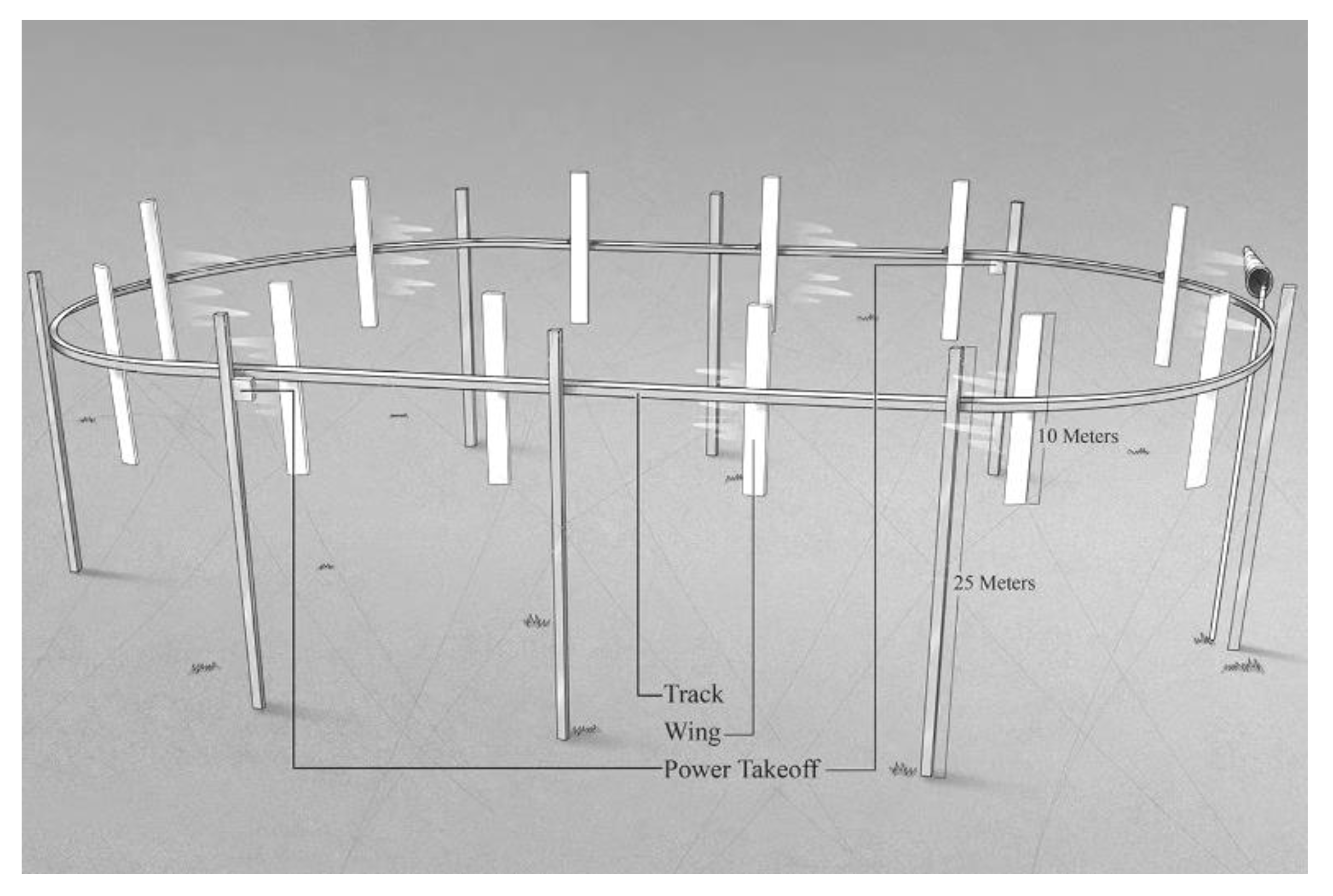
Figure 10.
Mechanism of flow deformation in a collinear turbine: a - turbine wind wheel, segregation of elementary segments; b – deformation of an elementary annular jet. Source [13].
Figure 10.
Mechanism of flow deformation in a collinear turbine: a - turbine wind wheel, segregation of elementary segments; b – deformation of an elementary annular jet. Source [13].
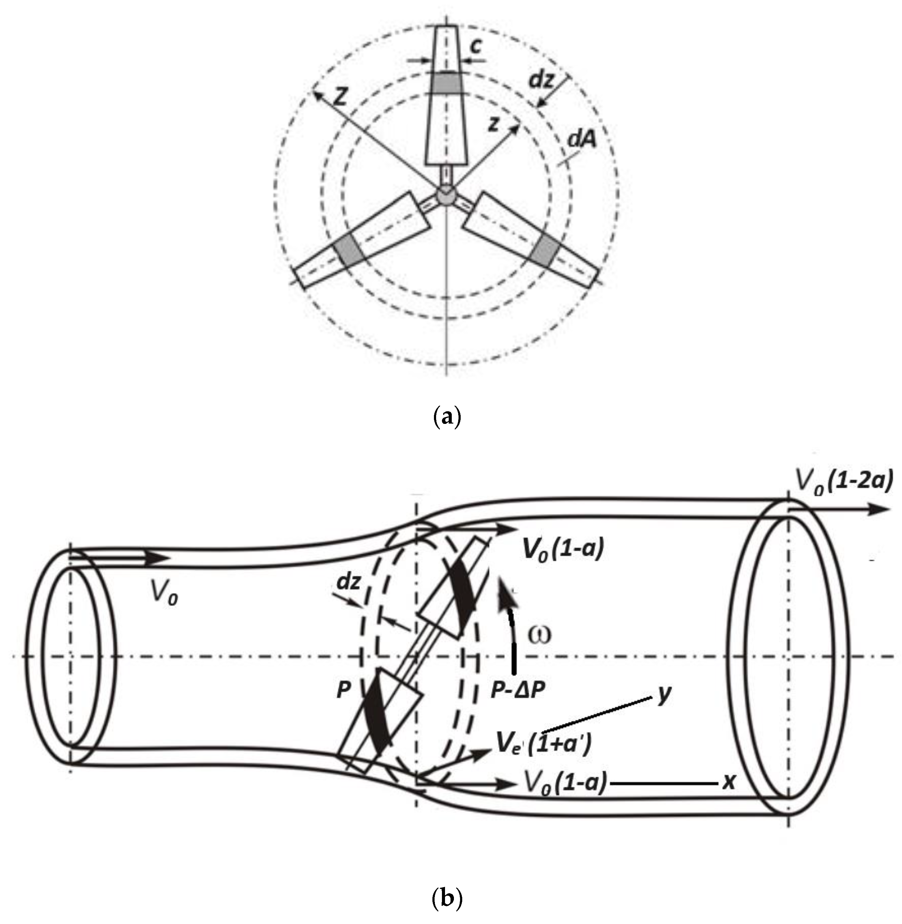
Figure 11.
Scheme of the interaction of a linear-convex blade with airflow.
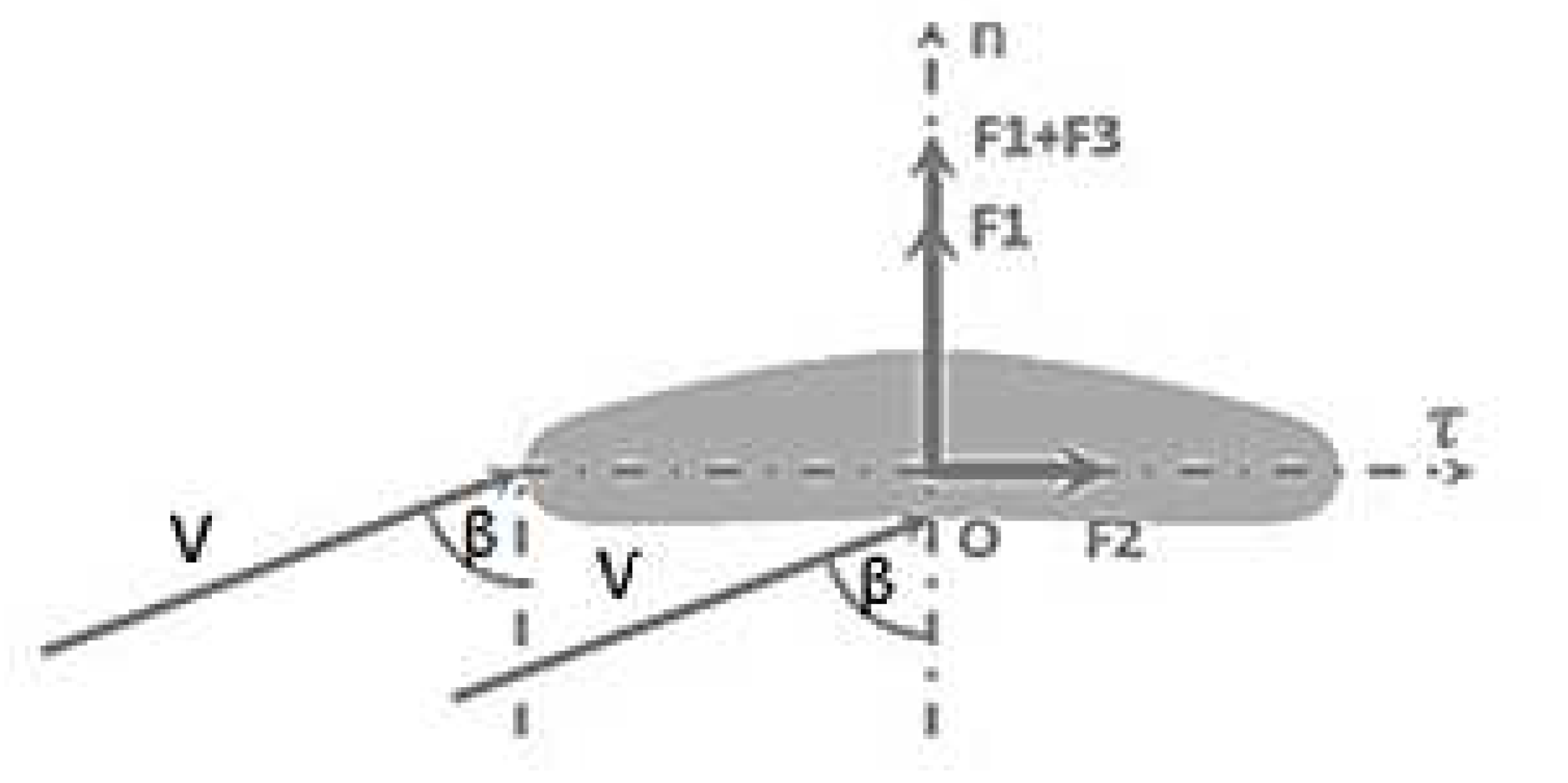
Figure 12.
Scheme of the interaction of the airflow with a segment of a collinear wind turbine: Ox is the main axis of the turbine, Oz is the longitudinal axis of the blade, z is the generalized coordinate of the segment, Ve is the nominal peripheral velocity of the segment.
Figure 12.
Scheme of the interaction of the airflow with a segment of a collinear wind turbine: Ox is the main axis of the turbine, Oz is the longitudinal axis of the blade, z is the generalized coordinate of the segment, Ve is the nominal peripheral velocity of the segment.
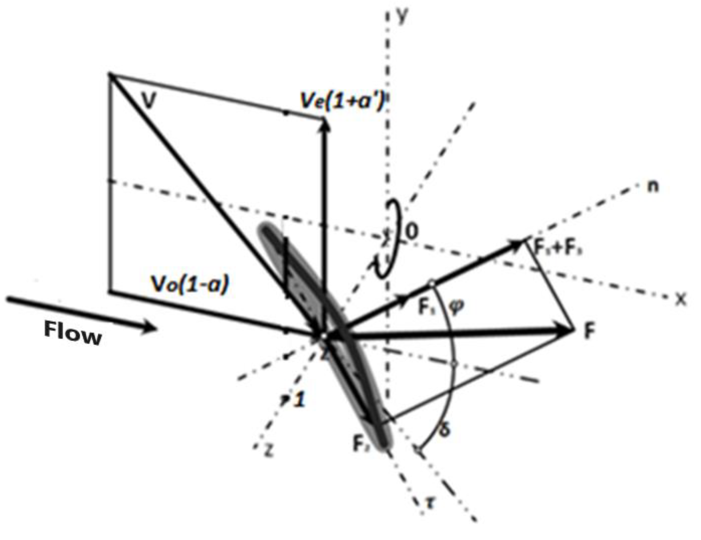
Figure 13.
Blade configuration characteristics.
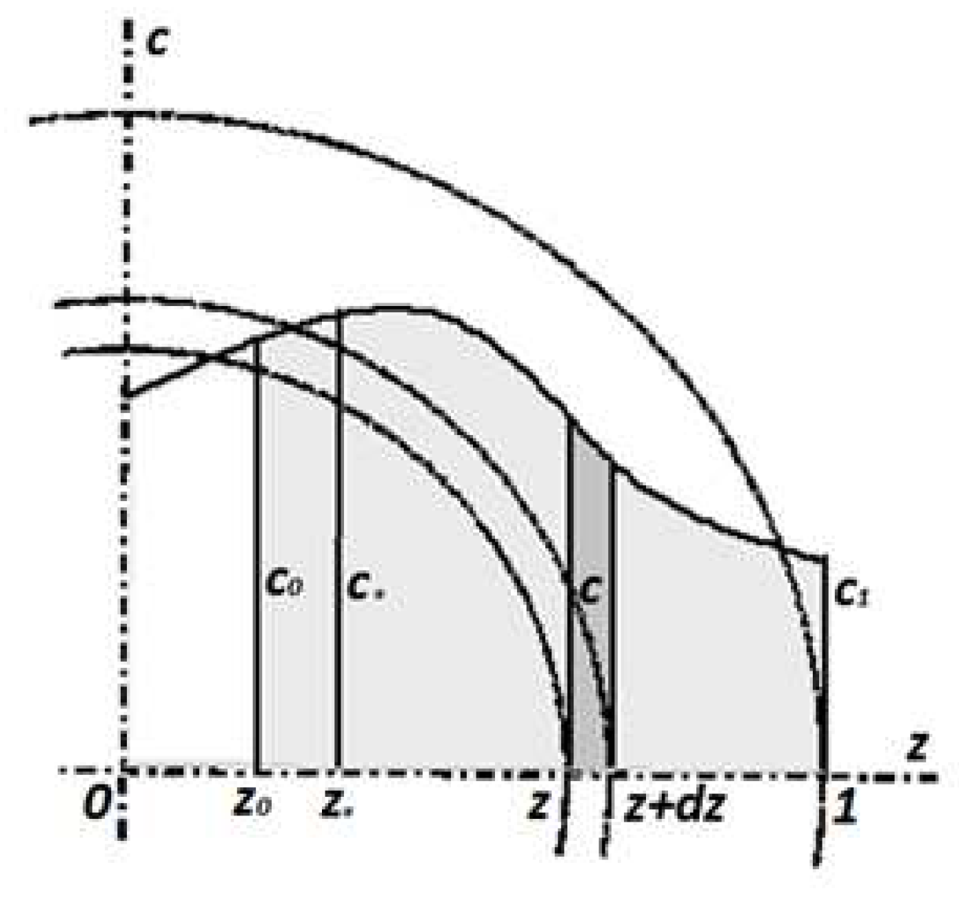
Figure 15.
Dependence of the optimal blade orientation angle φ of a collinear turbine on the direction angle of relative flow δ.
Figure 15.
Dependence of the optimal blade orientation angle φ of a collinear turbine on the direction angle of relative flow δ.
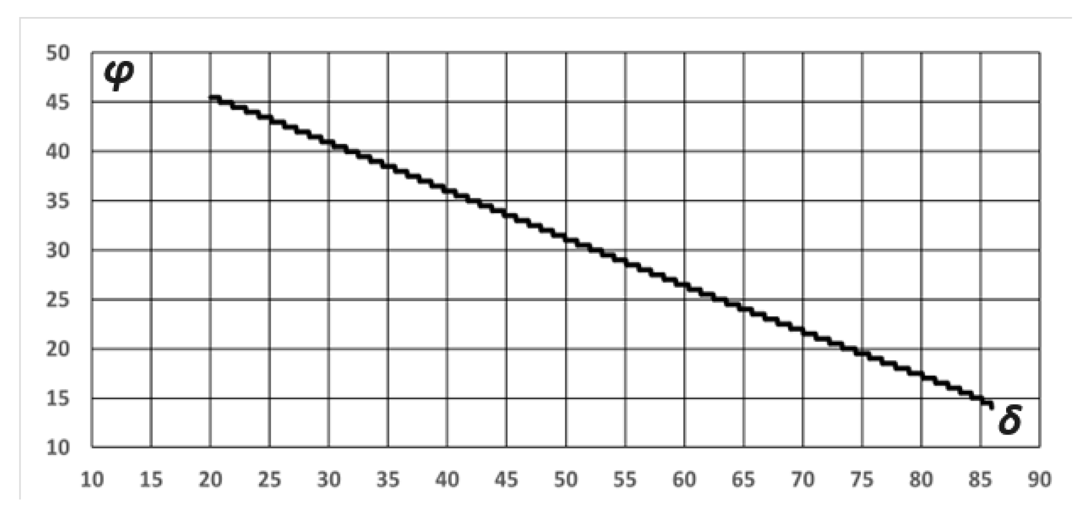
Figure 16.
Normalized blade shape characteristics: с – chord function; – an integral function of the area; σ – distribution of the area of elementary segments along the annular sections, a) linear expansion of the blade; b) uniform blade width; c) narrowing of the blade.
Figure 16.
Normalized blade shape characteristics: с – chord function; – an integral function of the area; σ – distribution of the area of elementary segments along the annular sections, a) linear expansion of the blade; b) uniform blade width; c) narrowing of the blade.
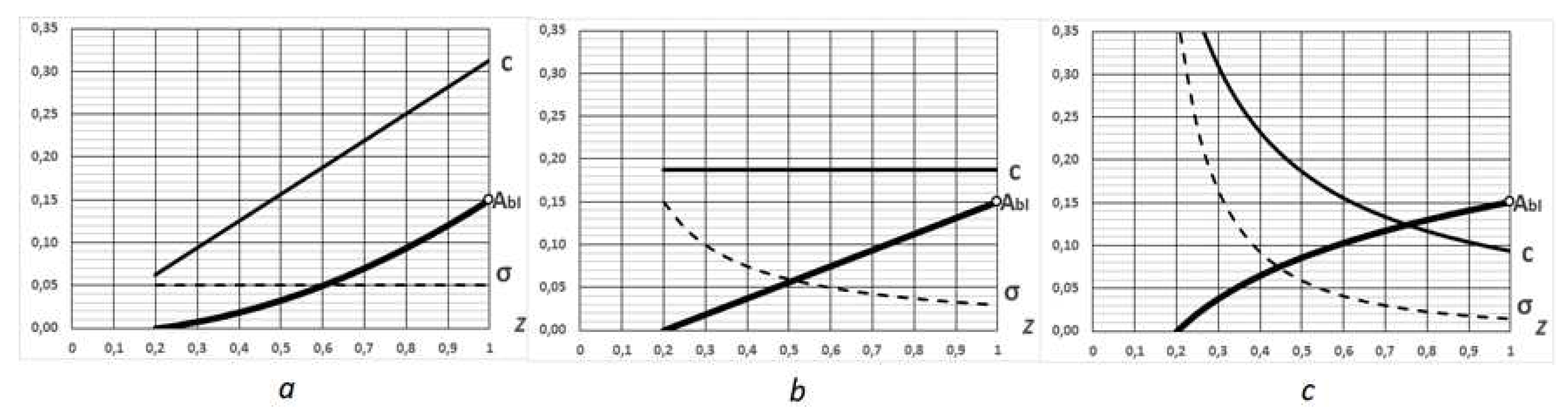
Figure 17.
View of the family of objective functions in modified Maalavi equations for collinear turbines.
Figure 17.
View of the family of objective functions in modified Maalavi equations for collinear turbines.
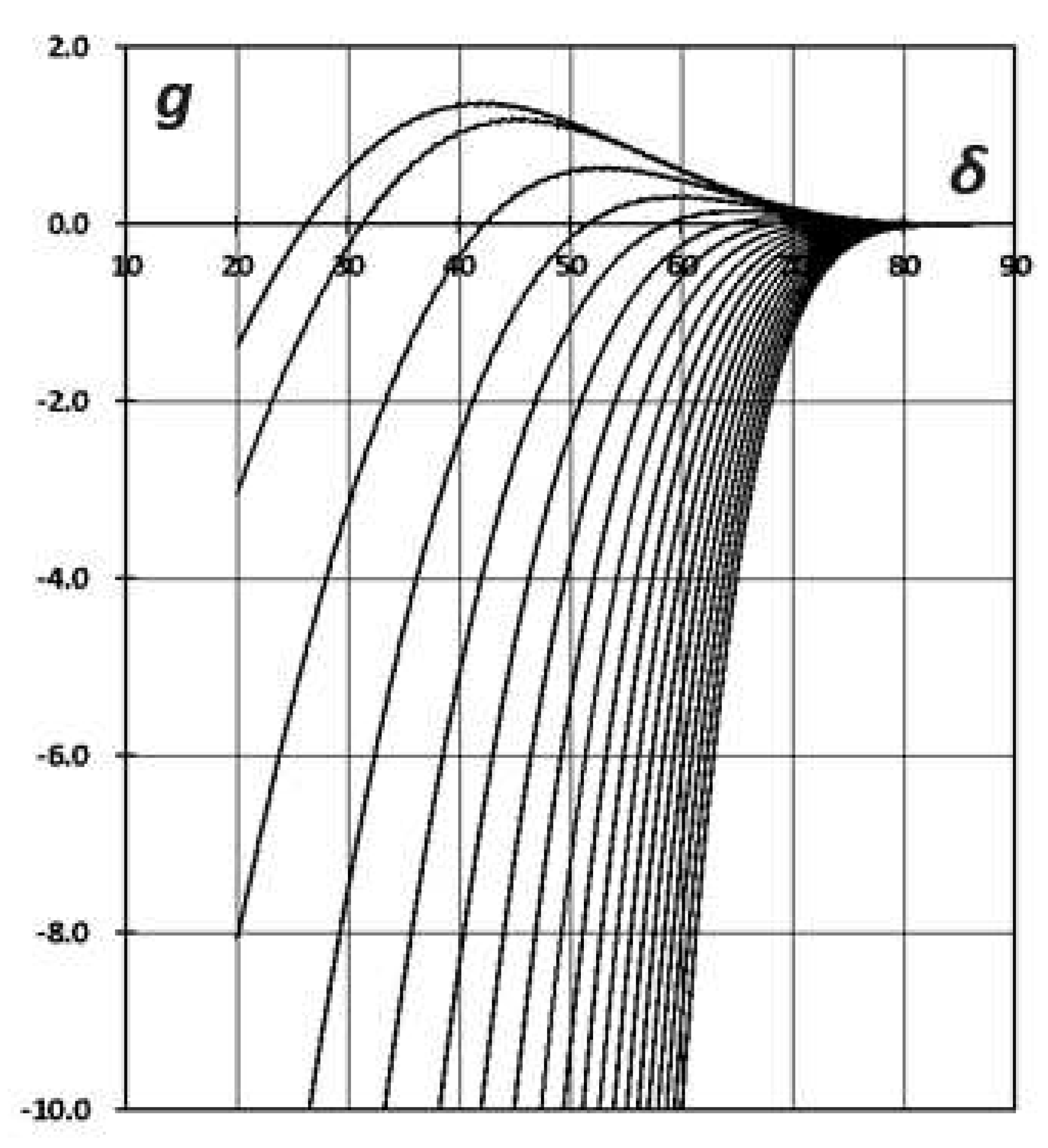
Figure 18.
Example of calculating optimal angles: the direction of relative flow δ; blade orientation φ, angles of attack ψ, depending on the blade cross-section z and speed coefficient λ1 - а) λ1=3; b) λ1=5; c) λ1=7.
Figure 18.
Example of calculating optimal angles: the direction of relative flow δ; blade orientation φ, angles of attack ψ, depending on the blade cross-section z and speed coefficient λ1 - а) λ1=3; b) λ1=5; c) λ1=7.
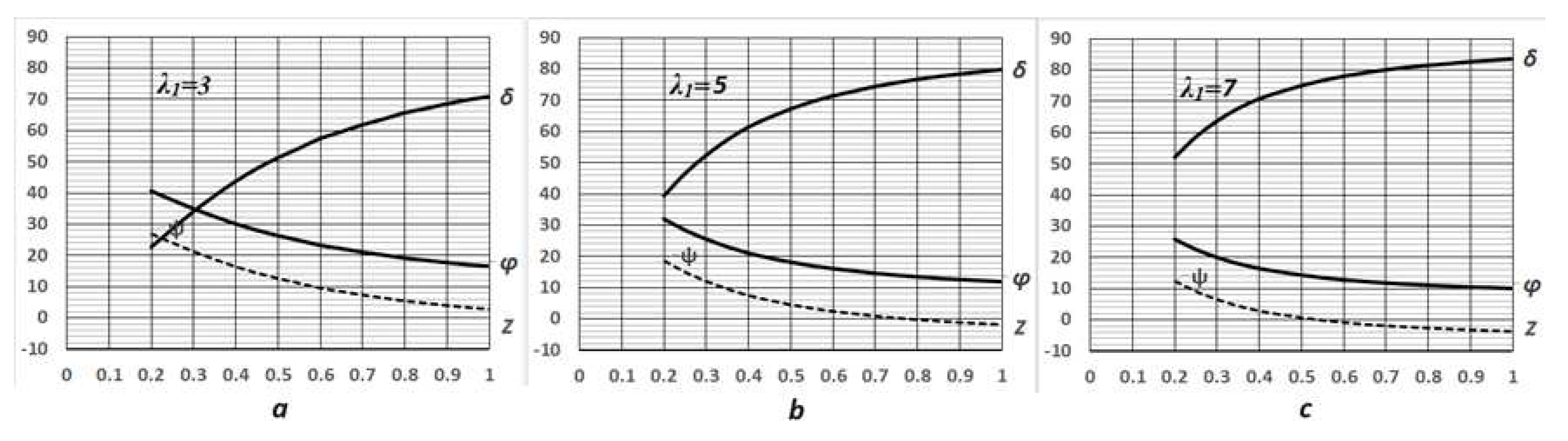
Figure 19.
Representation of an optimally configure d blade of a collinear turbine: V is the relative flow velocity vector, F is the vector of the applied resultant force.
Figure 19.
Representation of an optimally configure d blade of a collinear turbine: V is the relative flow velocity vector, F is the vector of the applied resultant force.
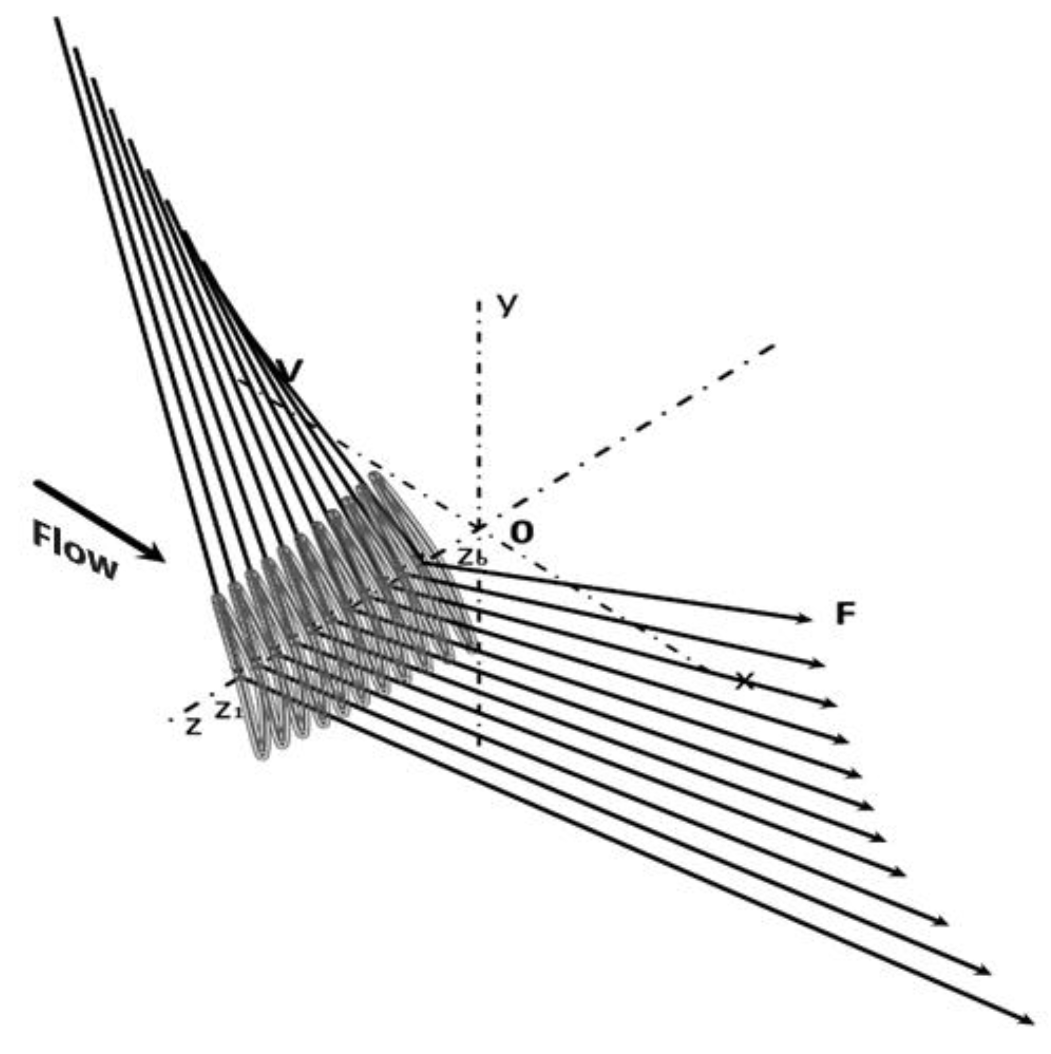
Figure 20.
Example of calculation of complex impact coefficients: longitudinal Cx, rotatory Cy, depending on the blade cross-section z and speed coefficient - а) λ1=3; b) λ1=5; c) λ1=7.
Figure 20.
Example of calculation of complex impact coefficients: longitudinal Cx, rotatory Cy, depending on the blade cross-section z and speed coefficient - а) λ1=3; b) λ1=5; c) λ1=7.
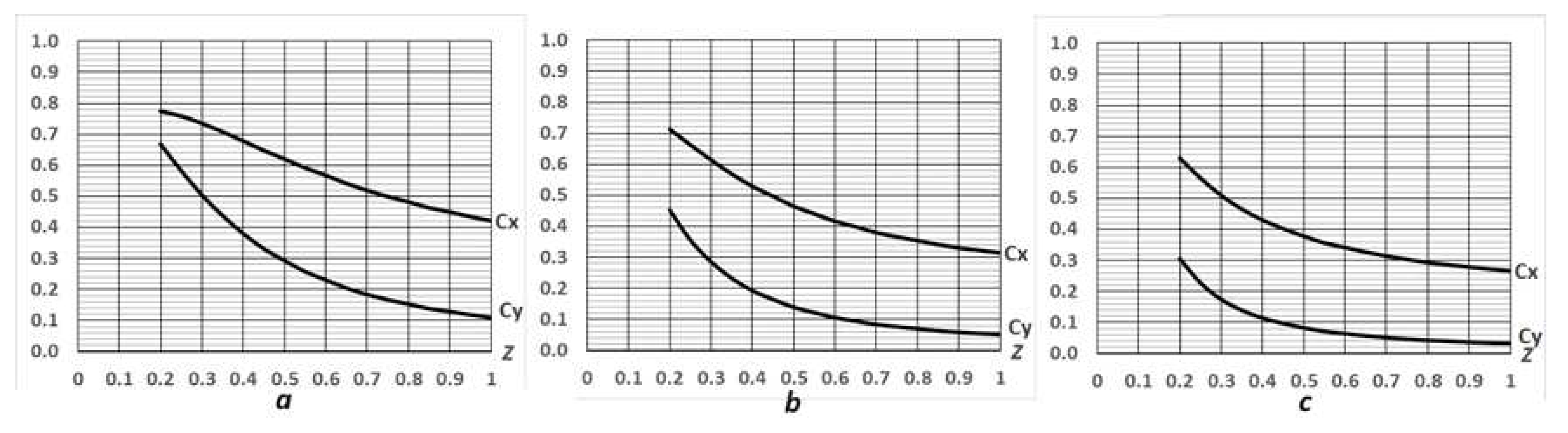
Figure 21.
An example of a typical distribution of calculated indicators: local induction coefficients a, power Cp, specific integral power Cpi, along the angular coordinate of the collinear turbine α - results of calculations using the considered method.
Figure 21.
An example of a typical distribution of calculated indicators: local induction coefficients a, power Cp, specific integral power Cpi, along the angular coordinate of the collinear turbine α - results of calculations using the considered method.
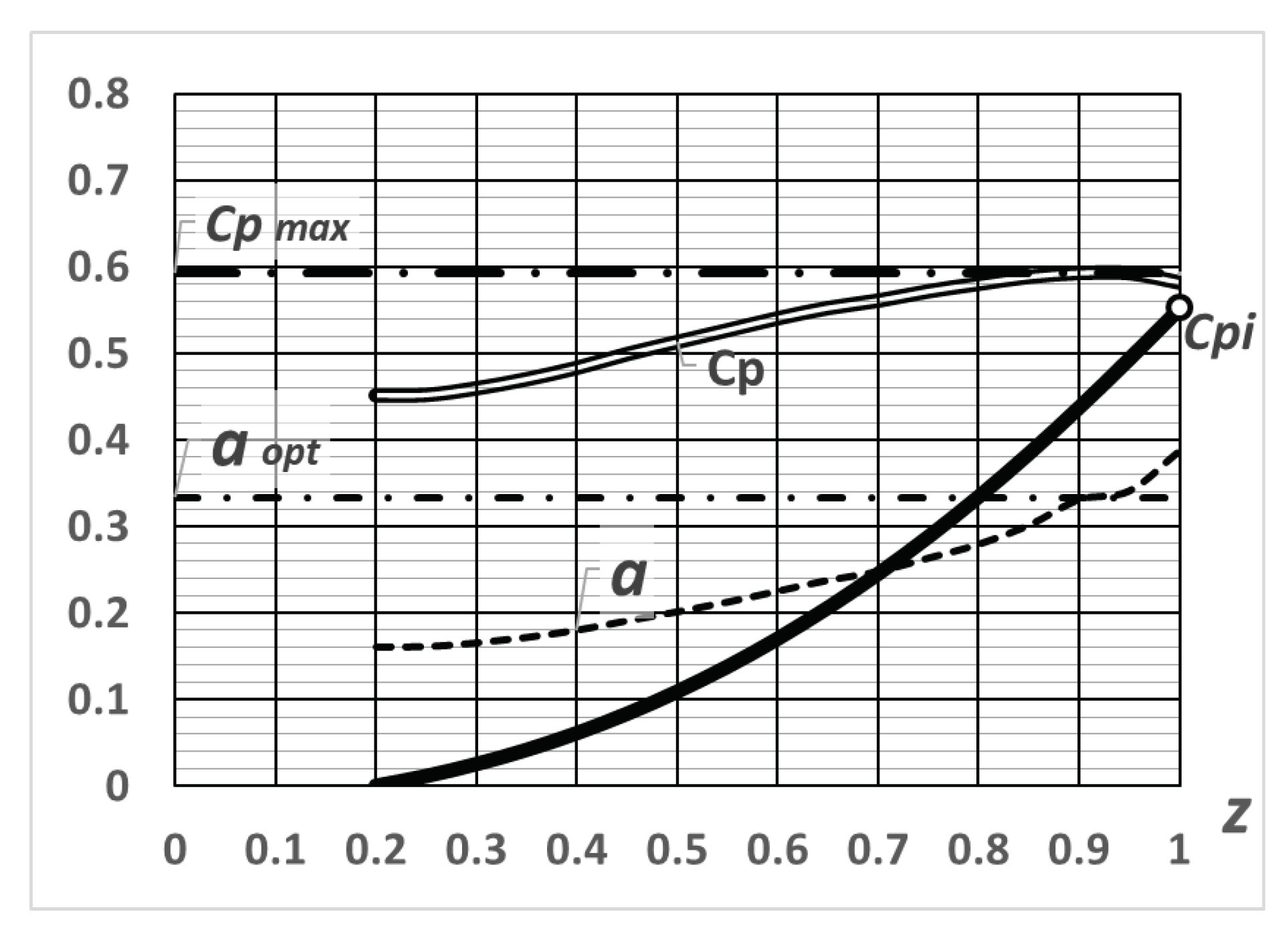
Figure 22.
Verification of the calculation methodology, a – comparison of blade geometry along the chord length: 1- proposed method [3], 2- source [15]; b – comparison of characteristic angles: 1- flow direction [14], 2- flow direction [15], 3- angle of attack [14], 4-angle of attack [15].
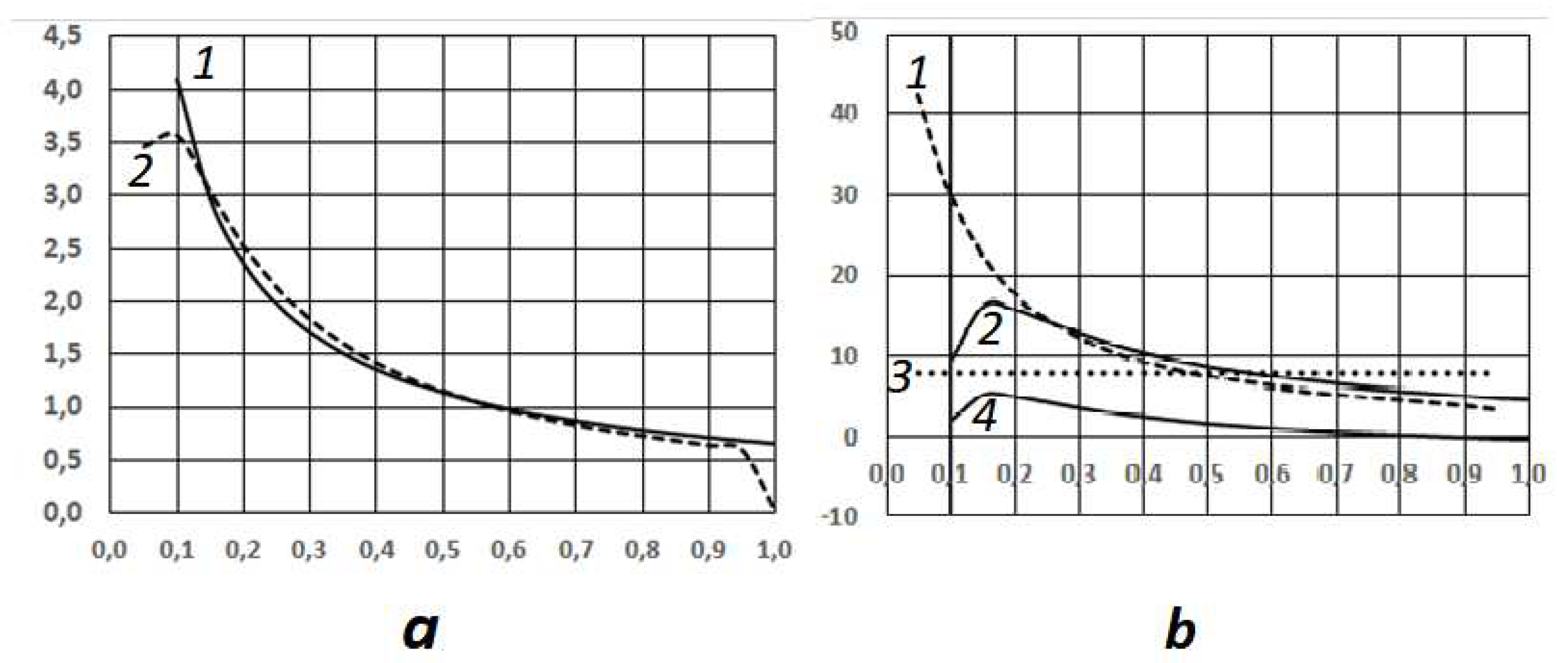
Figure 23.
Comparison of initial and optimized calculated data, the dependence of power factor on wind speed, points – experiment, line 1 – calculation from source [15], line 2 – calculation using the proposed method.
Figure 23.
Comparison of initial and optimized calculated data, the dependence of power factor on wind speed, points – experiment, line 1 – calculation from source [15], line 2 – calculation using the proposed method.
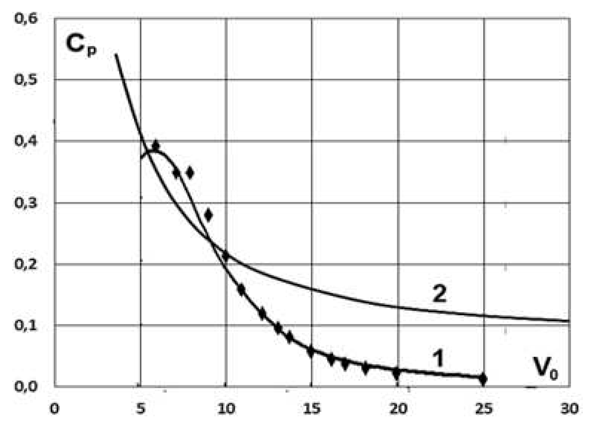
Figure 24.
The influence of blade shape on energy efficiency indicators: a) narrowing of the blade, n=-1; b) constant chord, n=0; c) linear expansion of the blade, n=1.
Figure 24.
The influence of blade shape on energy efficiency indicators: a) narrowing of the blade, n=-1; b) constant chord, n=0; c) linear expansion of the blade, n=1.
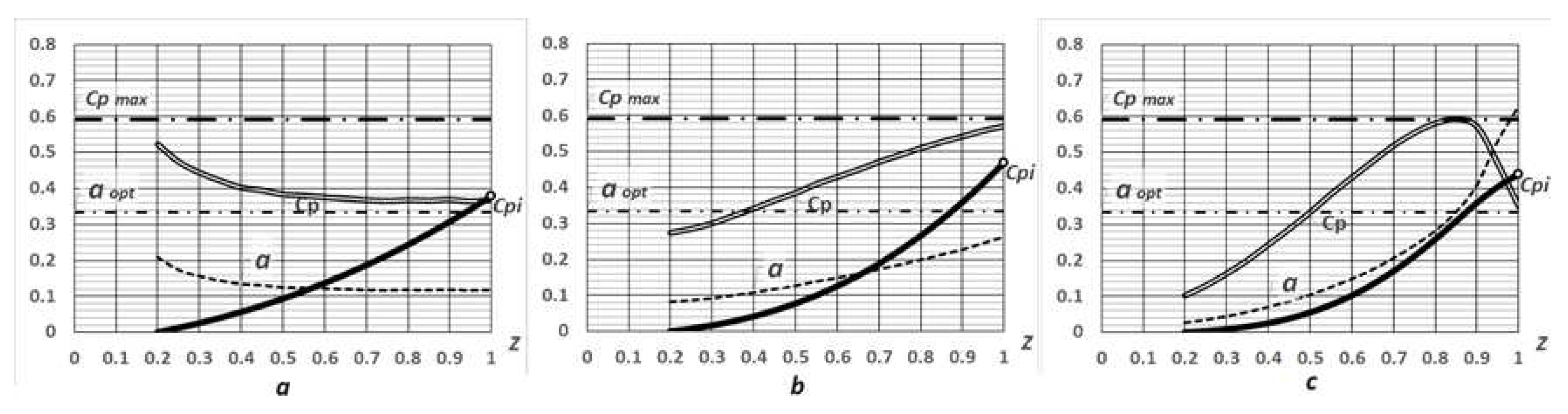
Figure 25.
The influence of blade area on energy efficiency indicators: the total area of the blades divided by the swept area of the turbine – а) =0.09; b) =0.12; c) =0.15.
Figure 25.
The influence of blade area on energy efficiency indicators: the total area of the blades divided by the swept area of the turbine – а) =0.09; b) =0.12; c) =0.15.
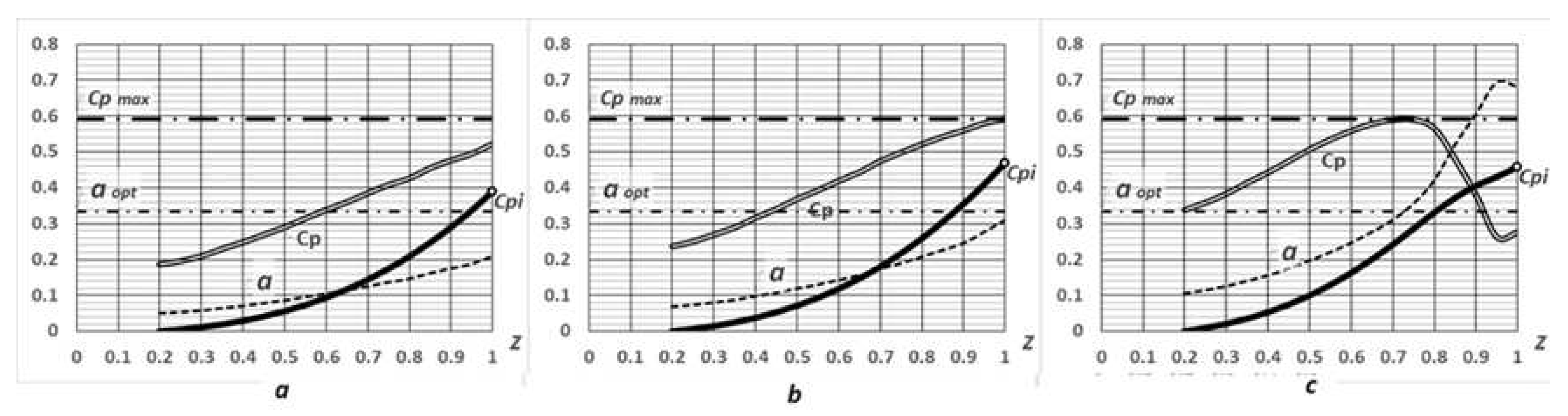
Figure 26.
The influence of turbine speed on performance energy efficiency: blade tip speed ratio to wind speed - - а) λ1=6; b) λ1=8; c) λ1=10.
Figure 26.
The influence of turbine speed on performance energy efficiency: blade tip speed ratio to wind speed - - а) λ1=6; b) λ1=8; c) λ1=10.
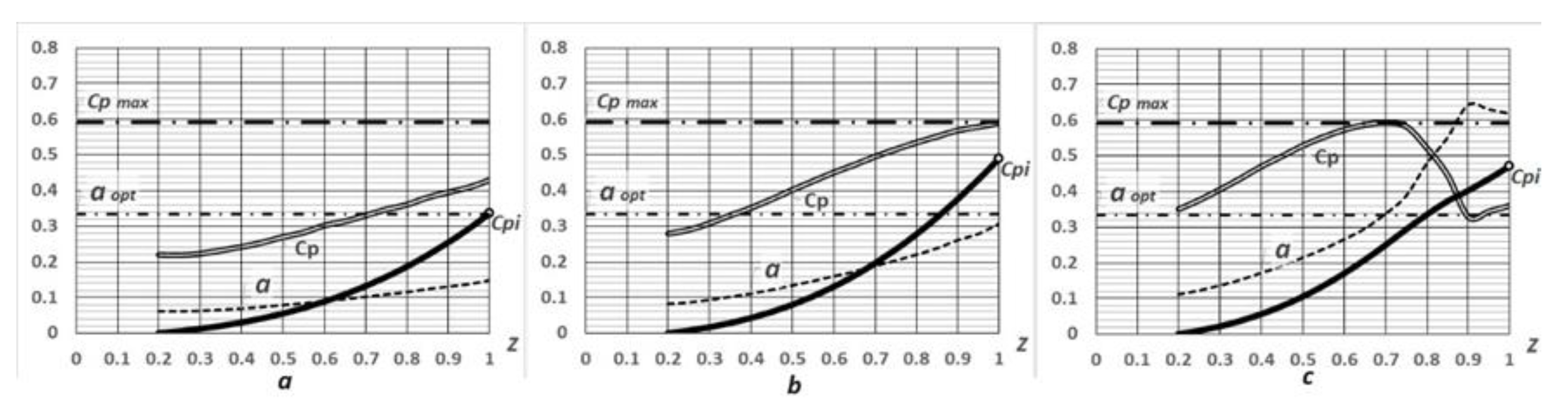
Figure 27.
Calculated characteristics "power factor - speed index" of a collinear turbine: tapering blades, shape factor n=-0.5; total blade density, line 1 – Abi= 0.15; line 2 - Abi= 0.05. Dashed lines – zones of the absence of roots of the Maalavi equations.
Figure 27.
Calculated characteristics "power factor - speed index" of a collinear turbine: tapering blades, shape factor n=-0.5; total blade density, line 1 – Abi= 0.15; line 2 - Abi= 0.05. Dashed lines – zones of the absence of roots of the Maalavi equations.
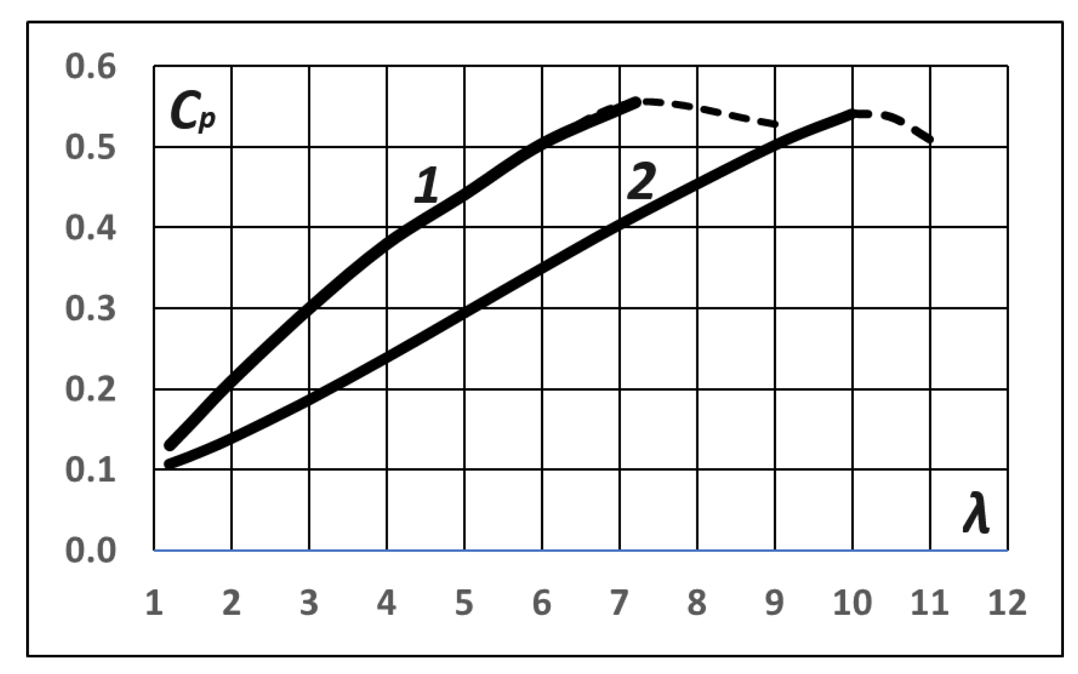
Figure 28.
Aerodynamic design of an orthogonal turbine: a – cylindrical turbine rotor; b – elementary deformation of the flat jet in sections – 1 - incoming flow, 2 - entrance to the cylindrical working zone, 3 - orthogonal diametrical section, 4 - exit from the cylindrical working zone, 5 - outgoing flow; diametrical cross-sections of the working cylinder - ABCD - orthogonal, EFGH - longitudinal.
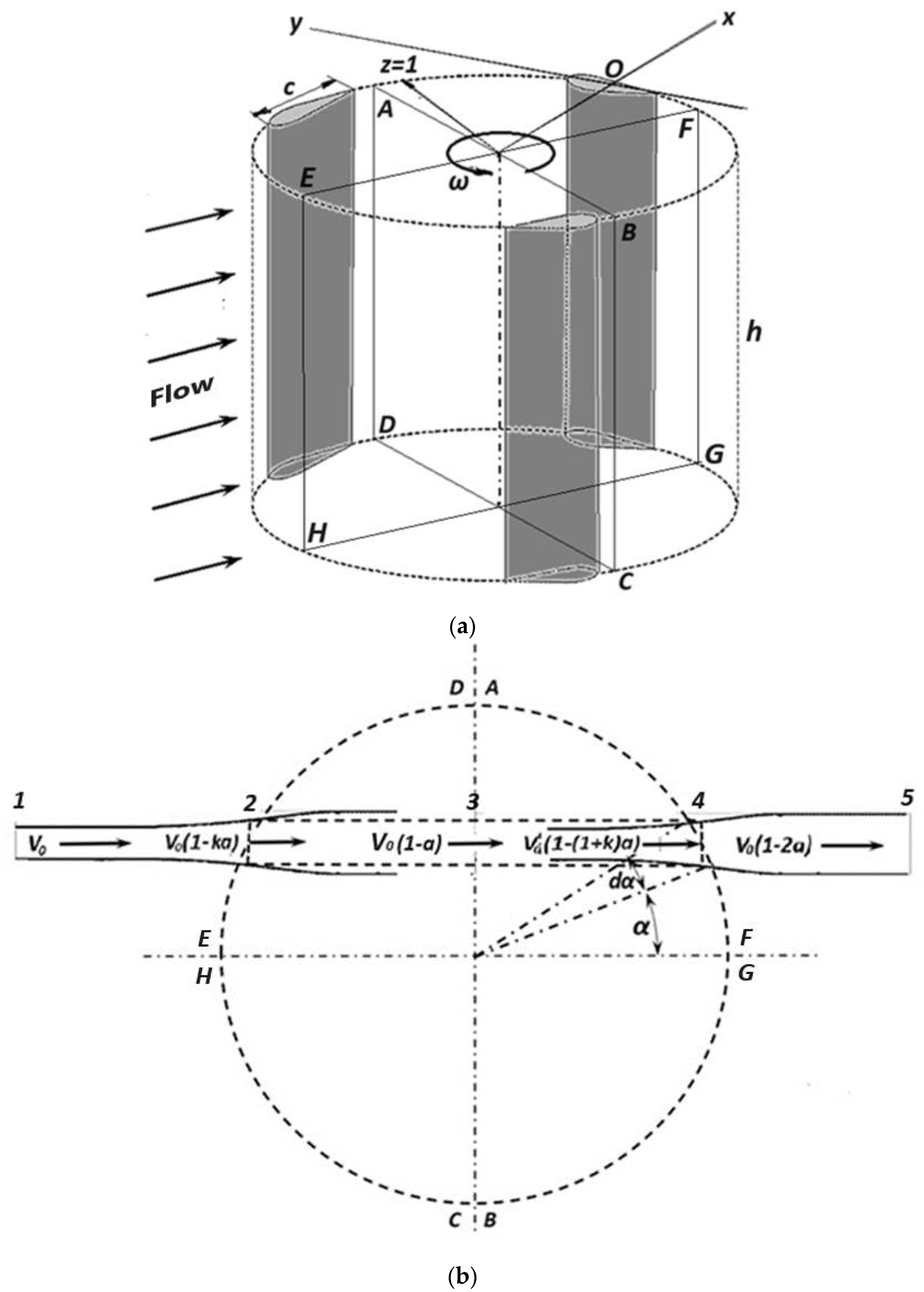
Figure 29.
Calculated values of the corrective index of induction ξ in sections of an elementary jet: NS – section number; lines 1-9 corresponding values of the local induction parameter k=0...1 with a step of 0.125.
Figure 29.
Calculated values of the corrective index of induction ξ in sections of an elementary jet: NS – section number; lines 1-9 corresponding values of the local induction parameter k=0...1 with a step of 0.125.
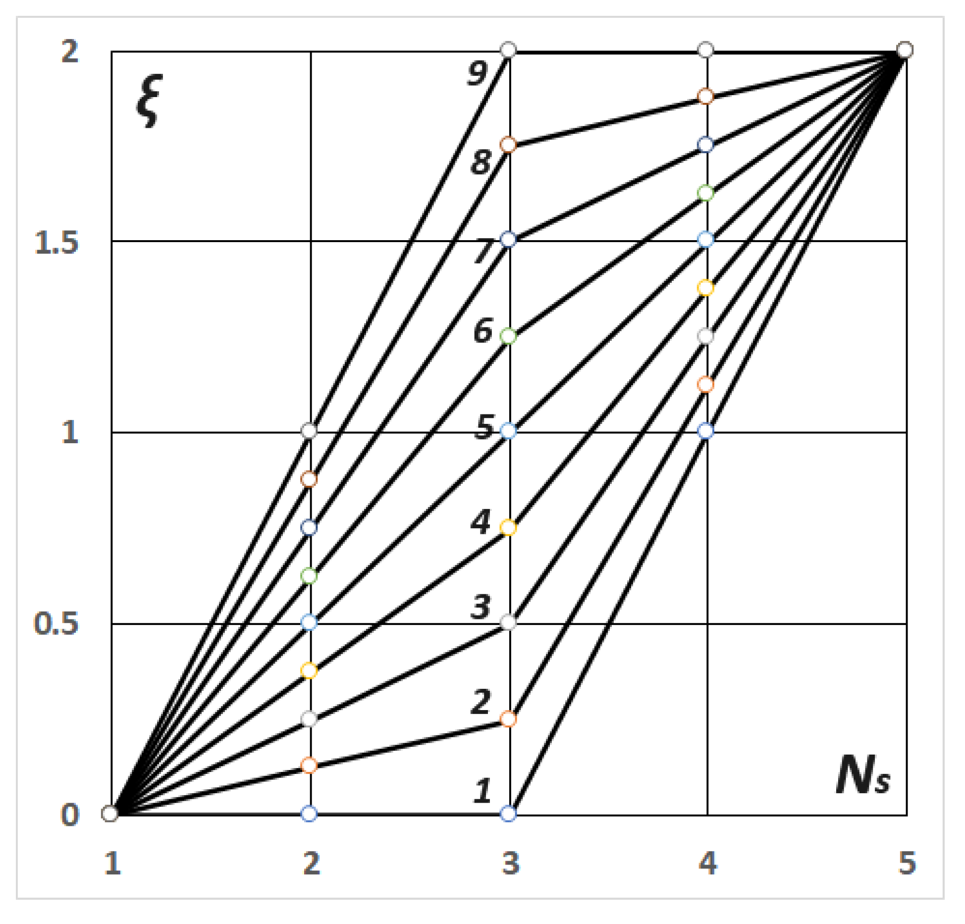
Figure 30.
Scheme of flow interaction with the blade of an orthogonal turbine : xOy – rotating coordinate system; α is the angular coordinate of the blade; δ – relative flow angle; φ – blade orientation angle; V0 – nominal (absolute) flow velocity; V – relative flow velocity; Ve – rotary (portable) velocity; F1, F2, F3 – aerodynamic forces.
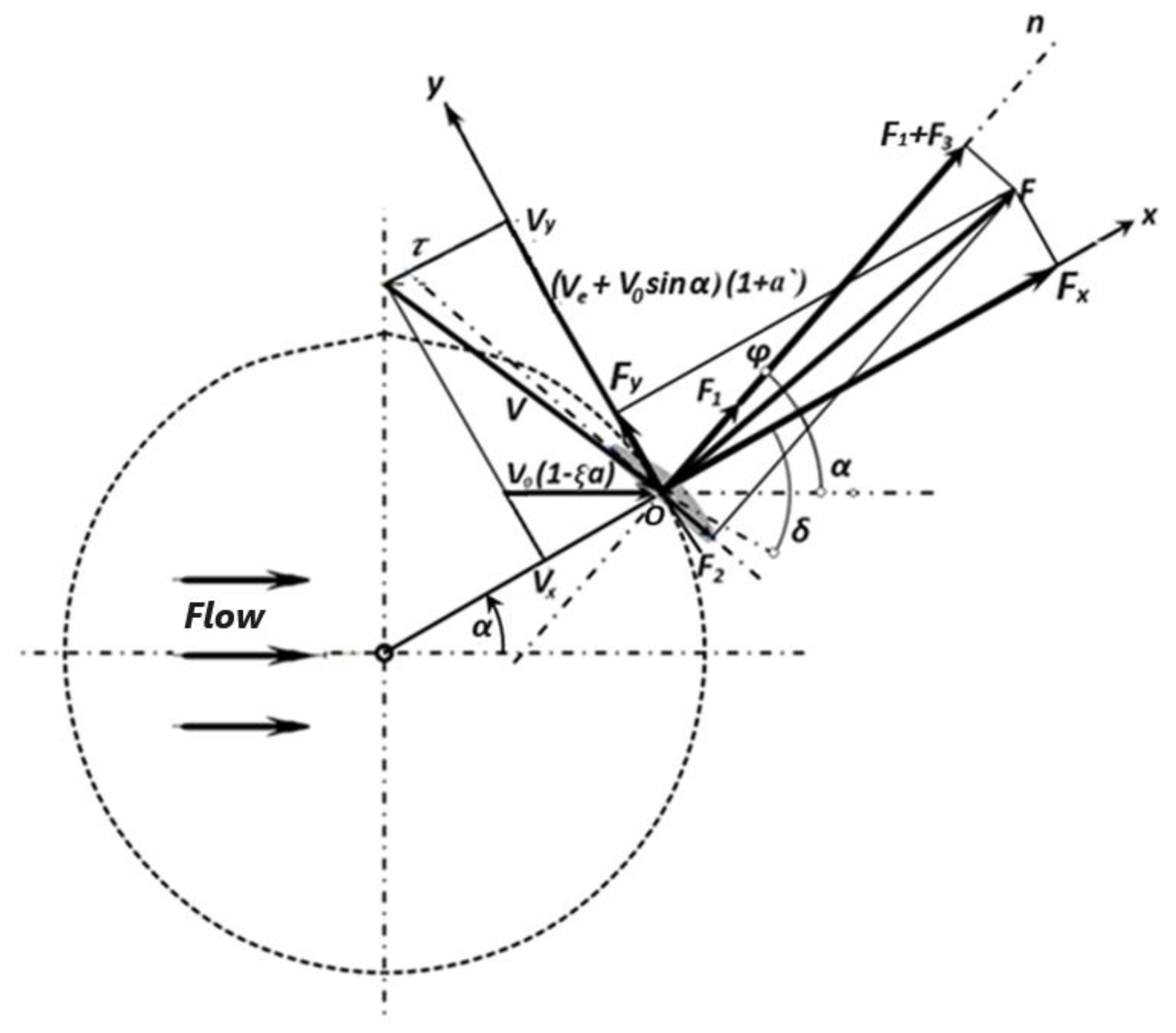
Figure 31.
Parametric families of a special function for an orthogonal turbine: at the top, the values of the parameter δ are significantly greater than -90o, then the intermediate ones are close to -90o, and at the bottom, they are significantly below -90o.
Figure 31.
Parametric families of a special function for an orthogonal turbine: at the top, the values of the parameter δ are significantly greater than -90o, then the intermediate ones are close to -90o, and at the bottom, they are significantly below -90o.
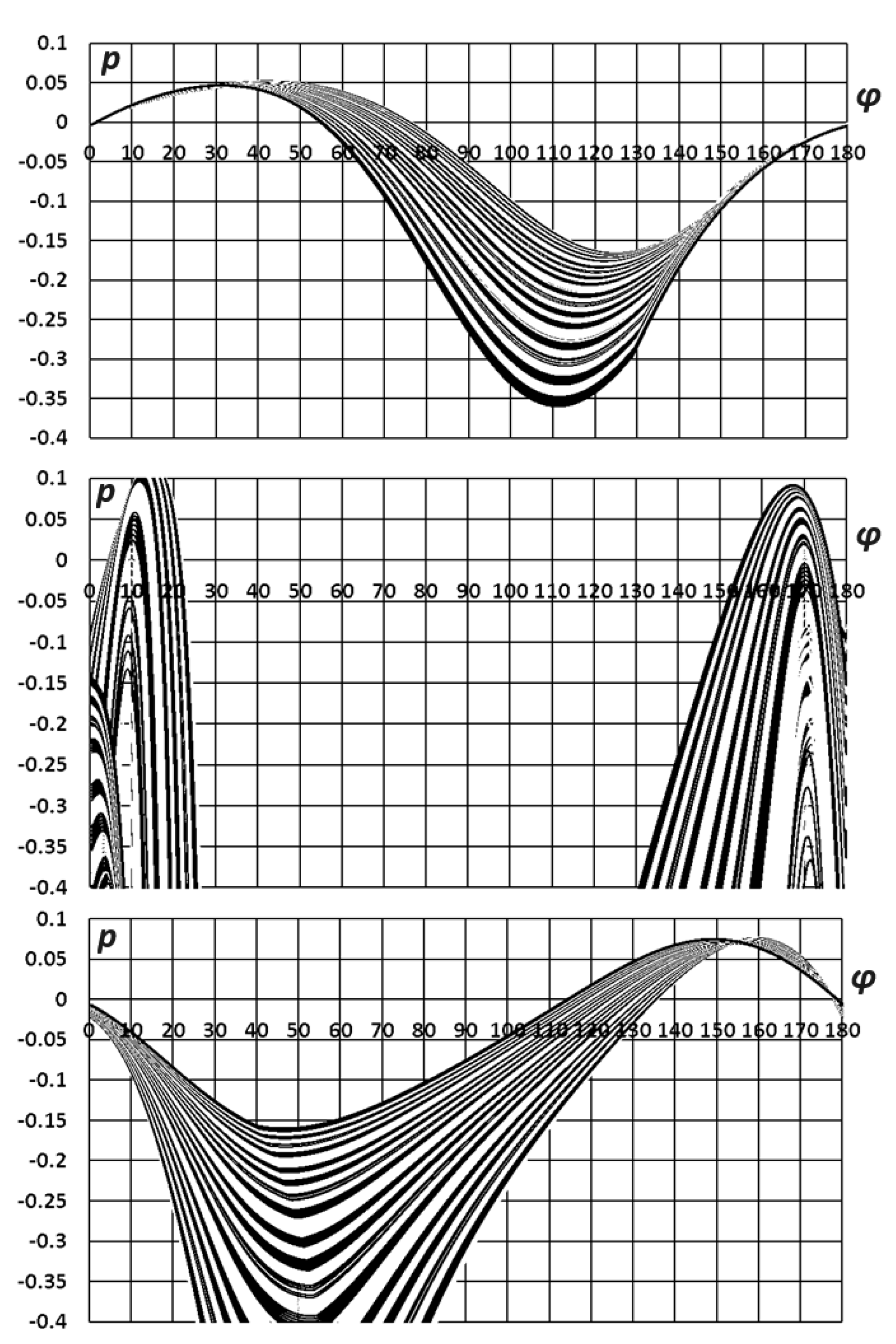
Figure 32.
Dependence of blade orientation angle φ orthogonal turbine on the relative flow direction angle δ. Inversion effect (abrupt change in blade orientation) - at a critical value of the characteristic angle .
Figure 32.
Dependence of blade orientation angle φ orthogonal turbine on the relative flow direction angle δ. Inversion effect (abrupt change in blade orientation) - at a critical value of the characteristic angle .
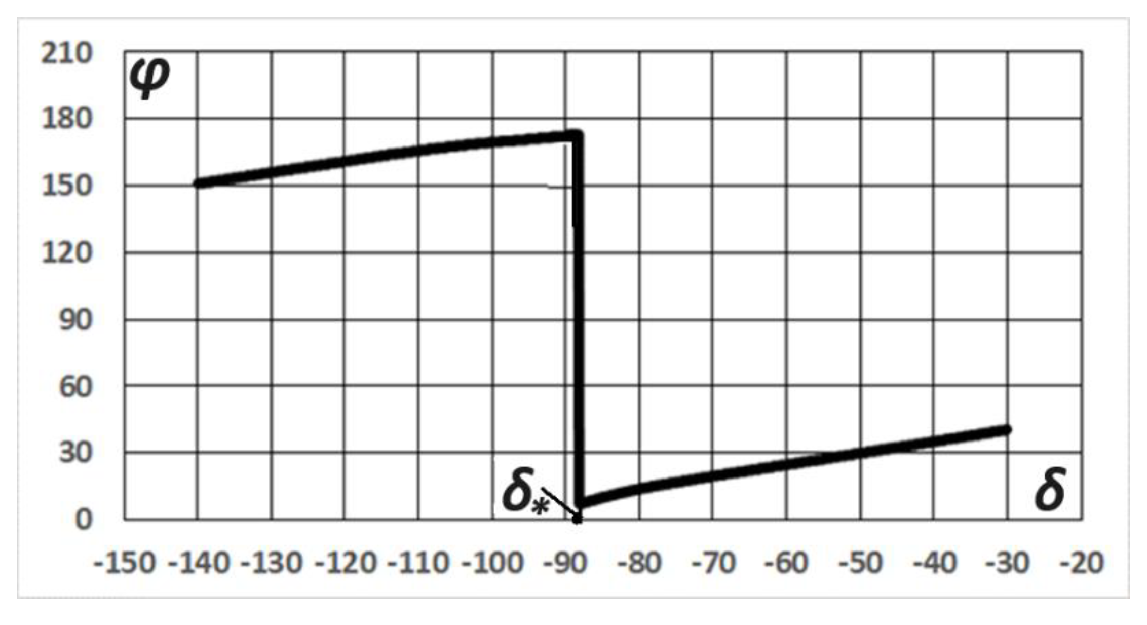
Figure 33.
View of the parametric family of objective functions g(δ,α) (parameter α) in modified Maalavi equations for orthogonal turbines.
Figure 33.
View of the parametric family of objective functions g(δ,α) (parameter α) in modified Maalavi equations for orthogonal turbines.
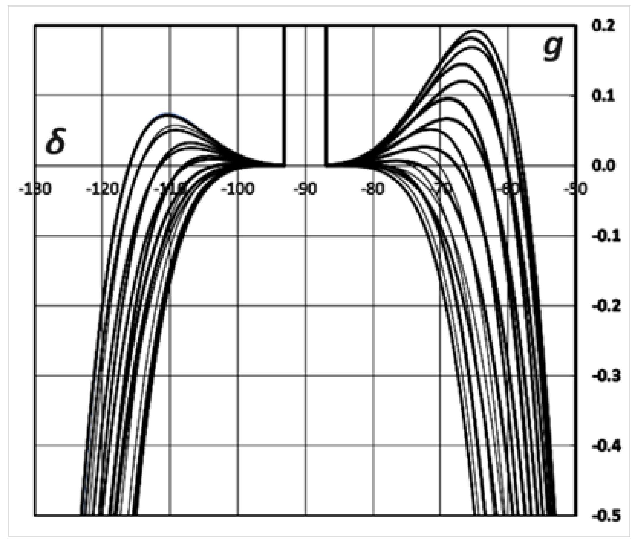
Figure 34.
Example of calculating optimal angles: the direction of relative flow δ; blade orientation φ, angles of attack ψ, depending on the angular coordinate of the blade α and speed index - а) λ=2; b) λ=4; c) λ=6.
Figure 34.
Example of calculating optimal angles: the direction of relative flow δ; blade orientation φ, angles of attack ψ, depending on the angular coordinate of the blade α and speed index - а) λ=2; b) λ=4; c) λ=6.
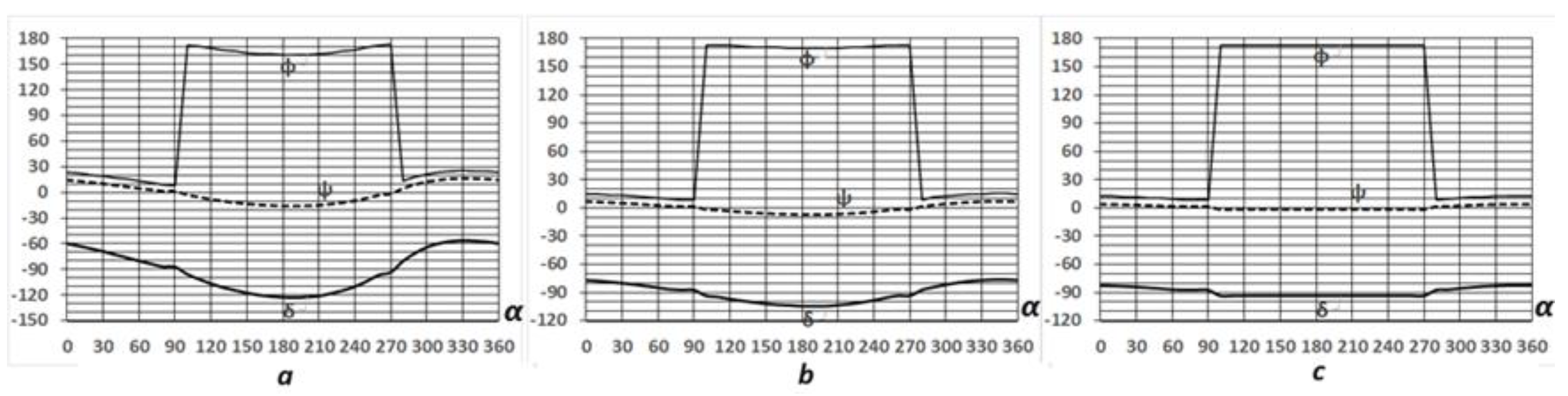
Figure 35.
Example of calculation of complex impact coefficients: radial Cx, rotary Cy, depending on the angular coordinate blade α and speed coefficient - а) λ=2; b) λ=4; c) λ=6.
Figure 35.
Example of calculation of complex impact coefficients: radial Cx, rotary Cy, depending on the angular coordinate blade α and speed coefficient - а) λ=2; b) λ=4; c) λ=6.
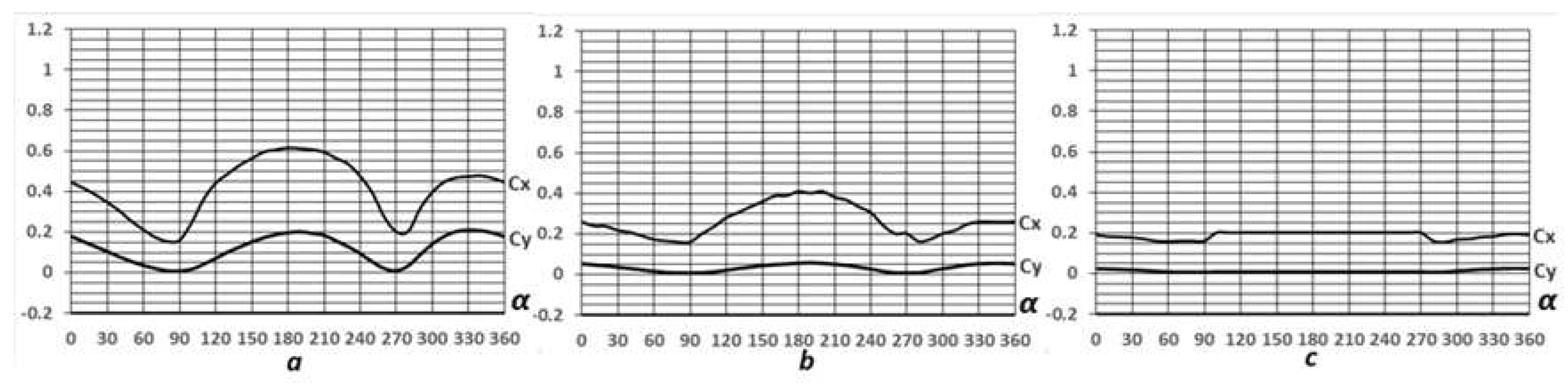
Figure 36.
An example of a typical distribution of calculated indicators: local induction coefficients a, power Cp, specific integral power Сpi, along the orthogonal angular coordinate turbines α – results of calculations using the considered method.
Figure 36.
An example of a typical distribution of calculated indicators: local induction coefficients a, power Cp, specific integral power Сpi, along the orthogonal angular coordinate turbines α – results of calculations using the considered method.
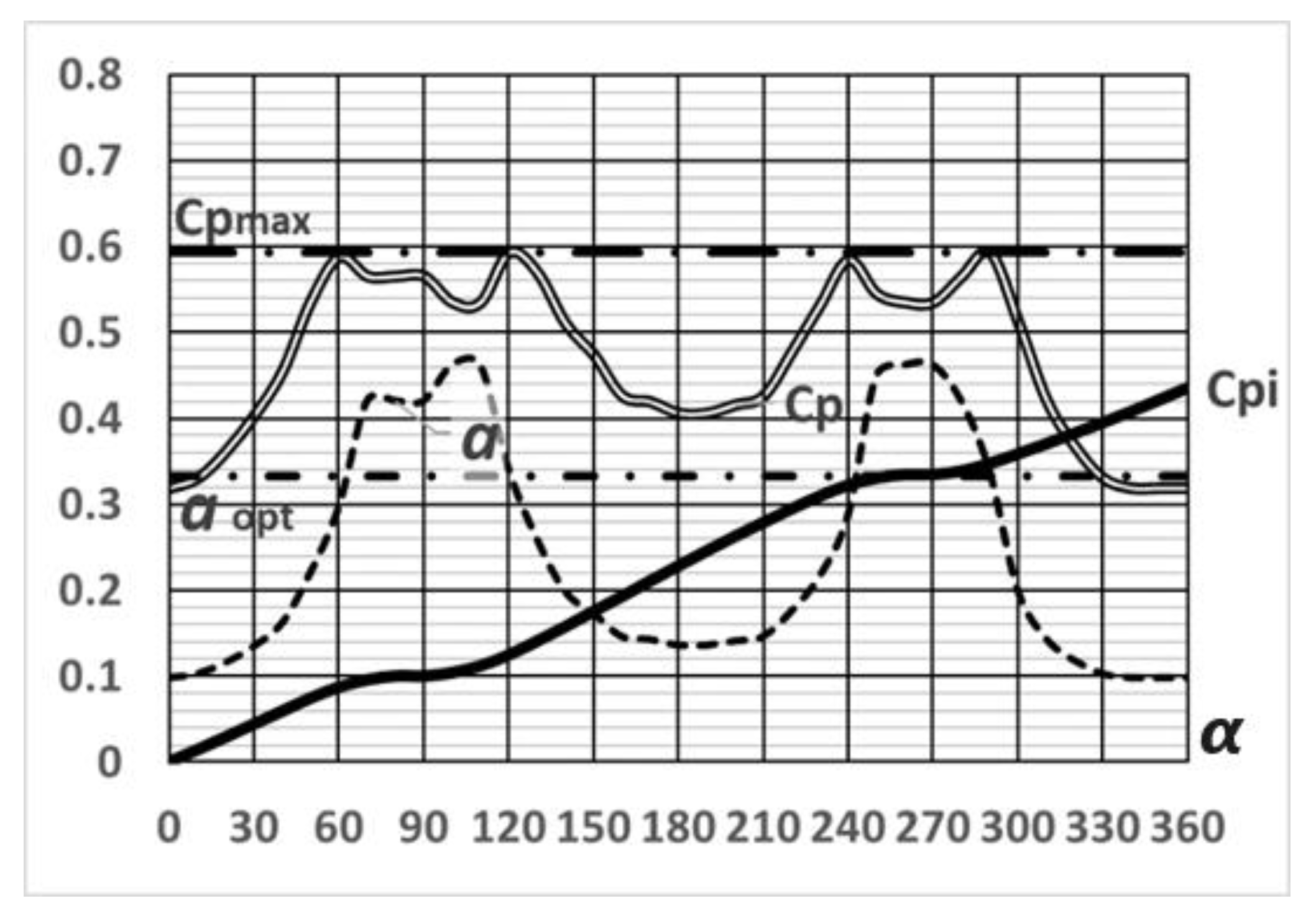
Figure 37.
Representation of an optimally oriented blade of orthogonal turbine: V – vector of relative flow velocity, F is the vector of the applied resultant force, The areas of blade inversion at angular coordinates α are highlighted: near 90o (top) and near 270o (bottom).
Figure 37.
Representation of an optimally oriented blade of orthogonal turbine: V – vector of relative flow velocity, F is the vector of the applied resultant force, The areas of blade inversion at angular coordinates α are highlighted: near 90o (top) and near 270o (bottom).
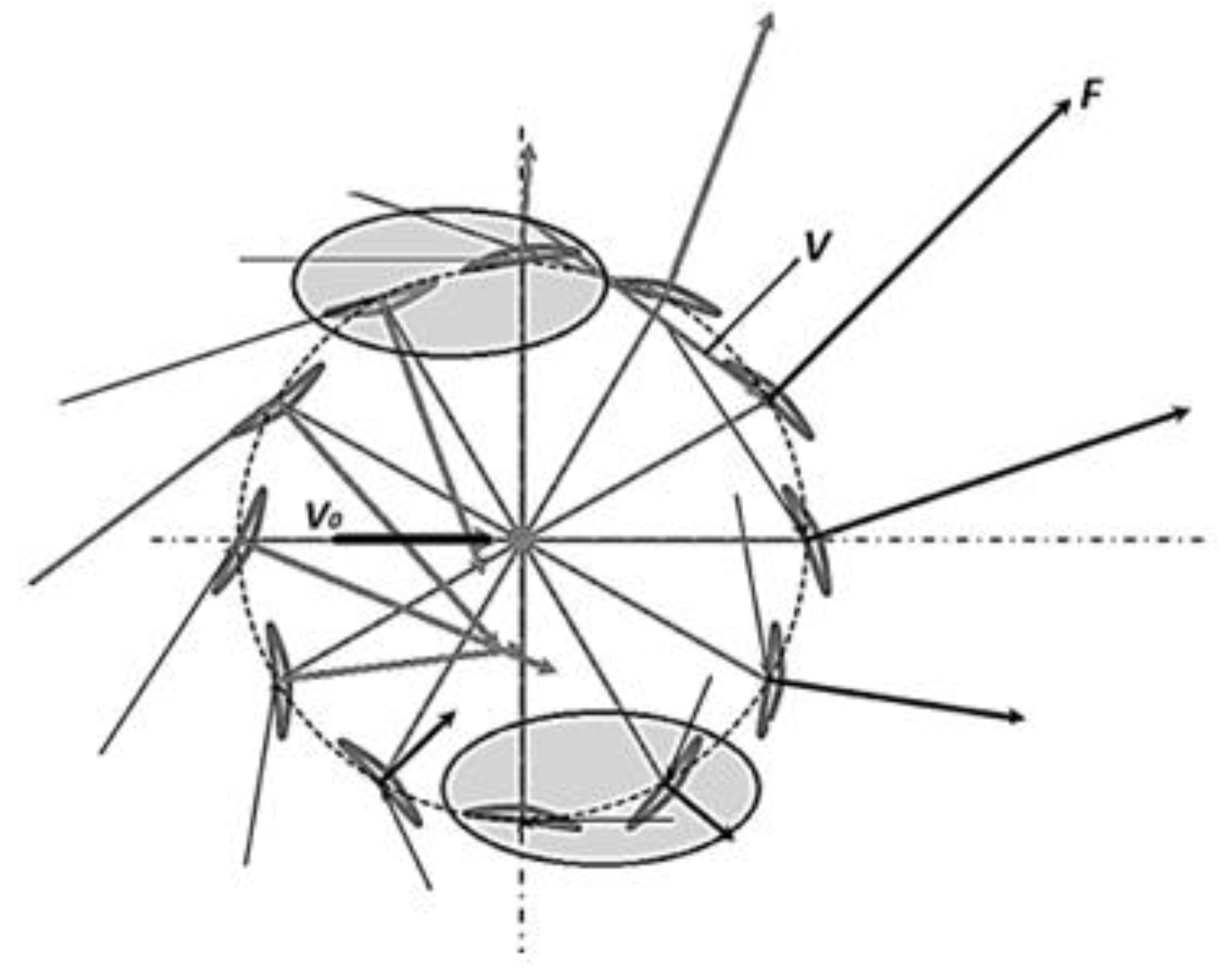
Figure 38.
Aerodynamic mechanism inversion of adjustable linear-convex blade.
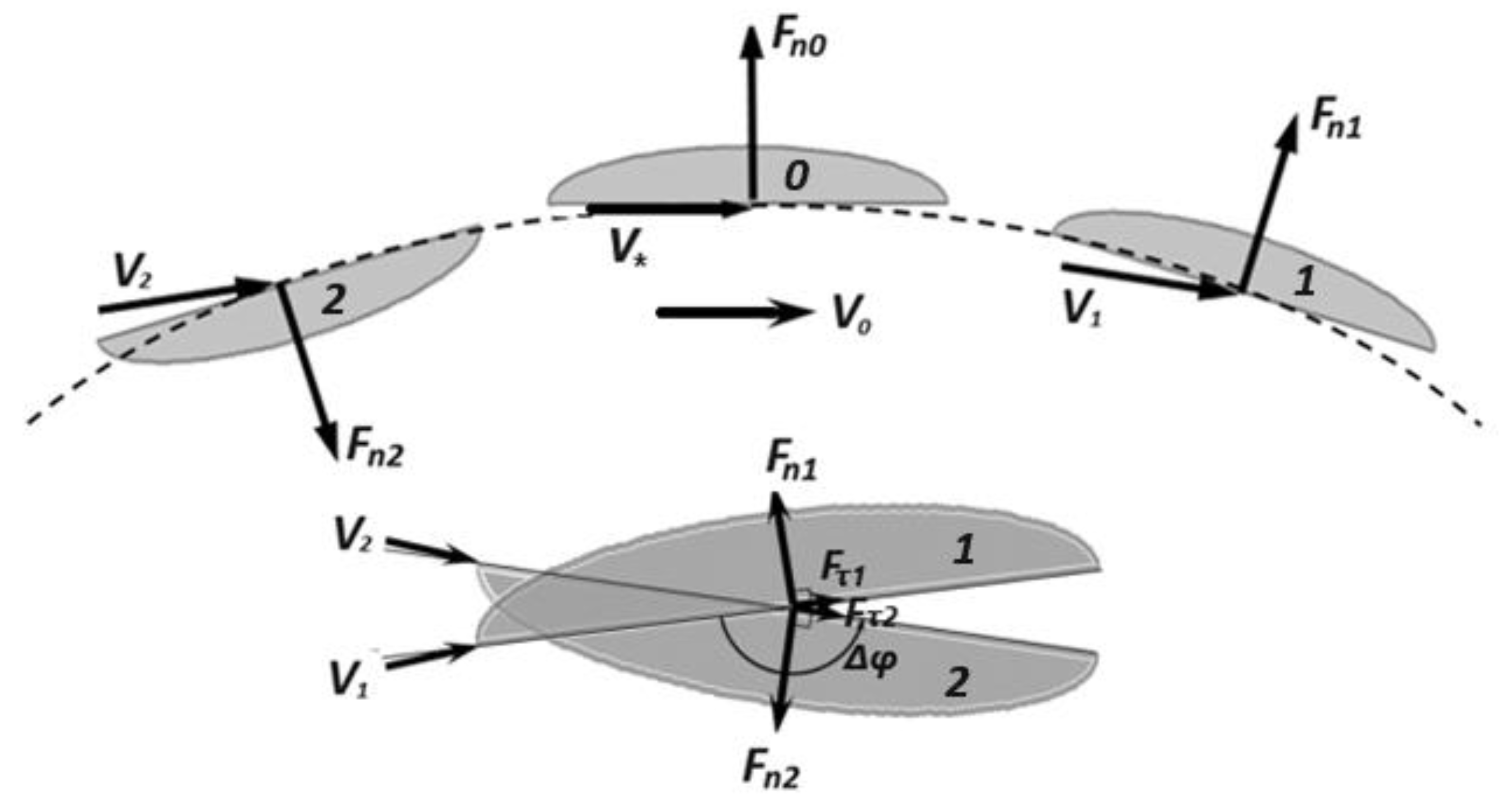
Figure 39.
Aerodynamic model of a symmetrical blade: µ - blade opening angle, ϑ - flow asymmetry angle.
Figure 39.
Aerodynamic model of a symmetrical blade: µ - blade opening angle, ϑ - flow asymmetry angle.
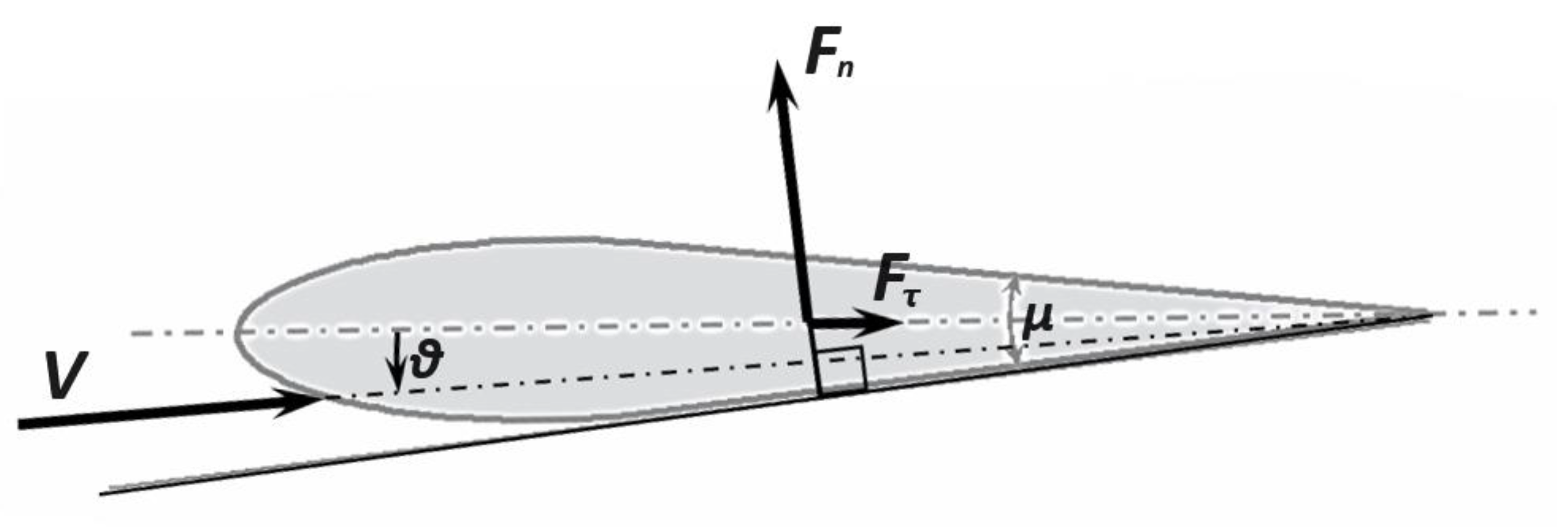
Figure 40.
Dependence of the lift coefficient s on asymmetry flow ϑ: 1 – sinusoidal-linear; 2 – piecewise linear; 3 – sign function.
Figure 40.
Dependence of the lift coefficient s on asymmetry flow ϑ: 1 – sinusoidal-linear; 2 – piecewise linear; 3 – sign function.
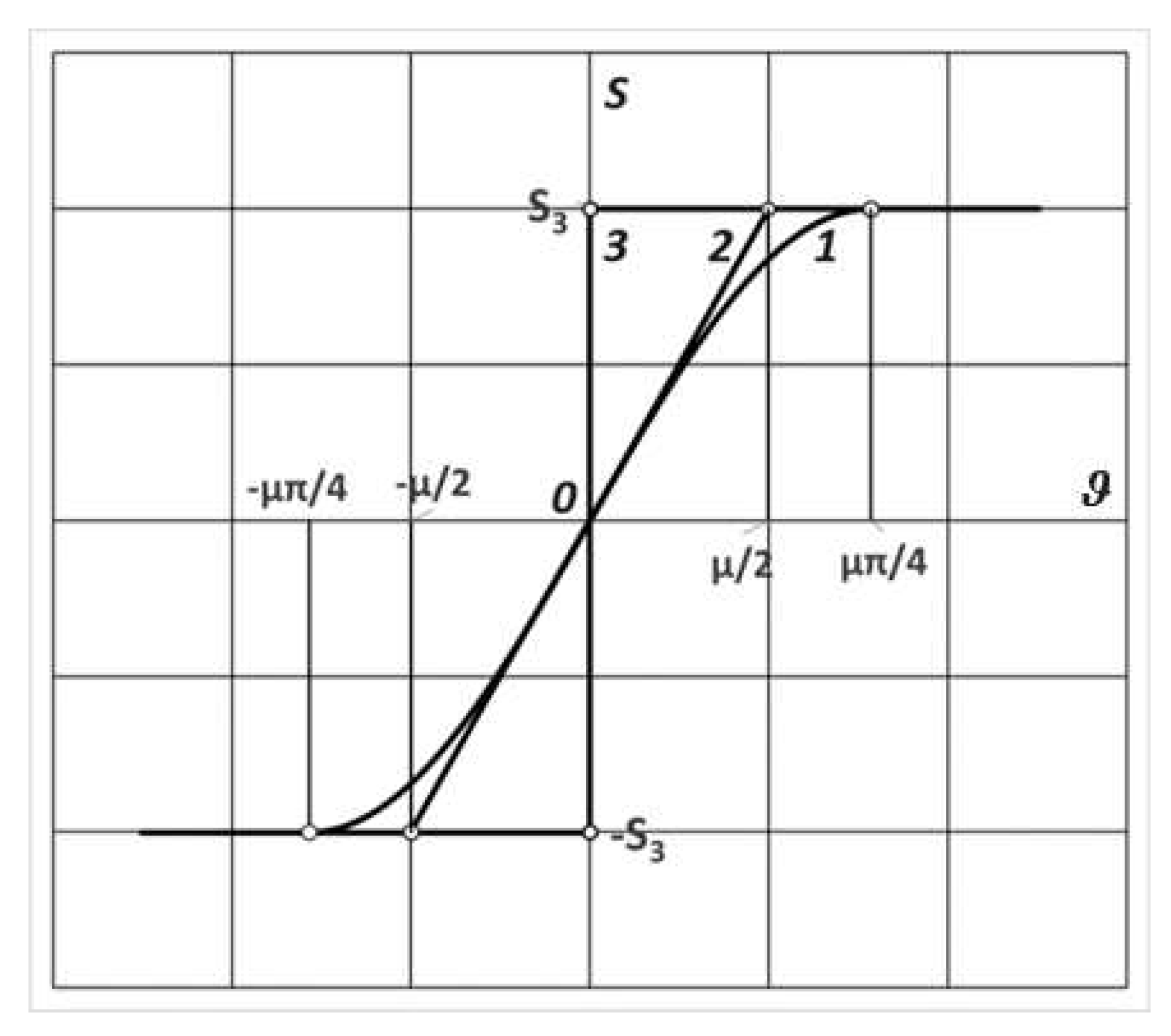
Figure 41.
Aerodynamic mechanism of reverse inversion adjustable symmetrical blade.
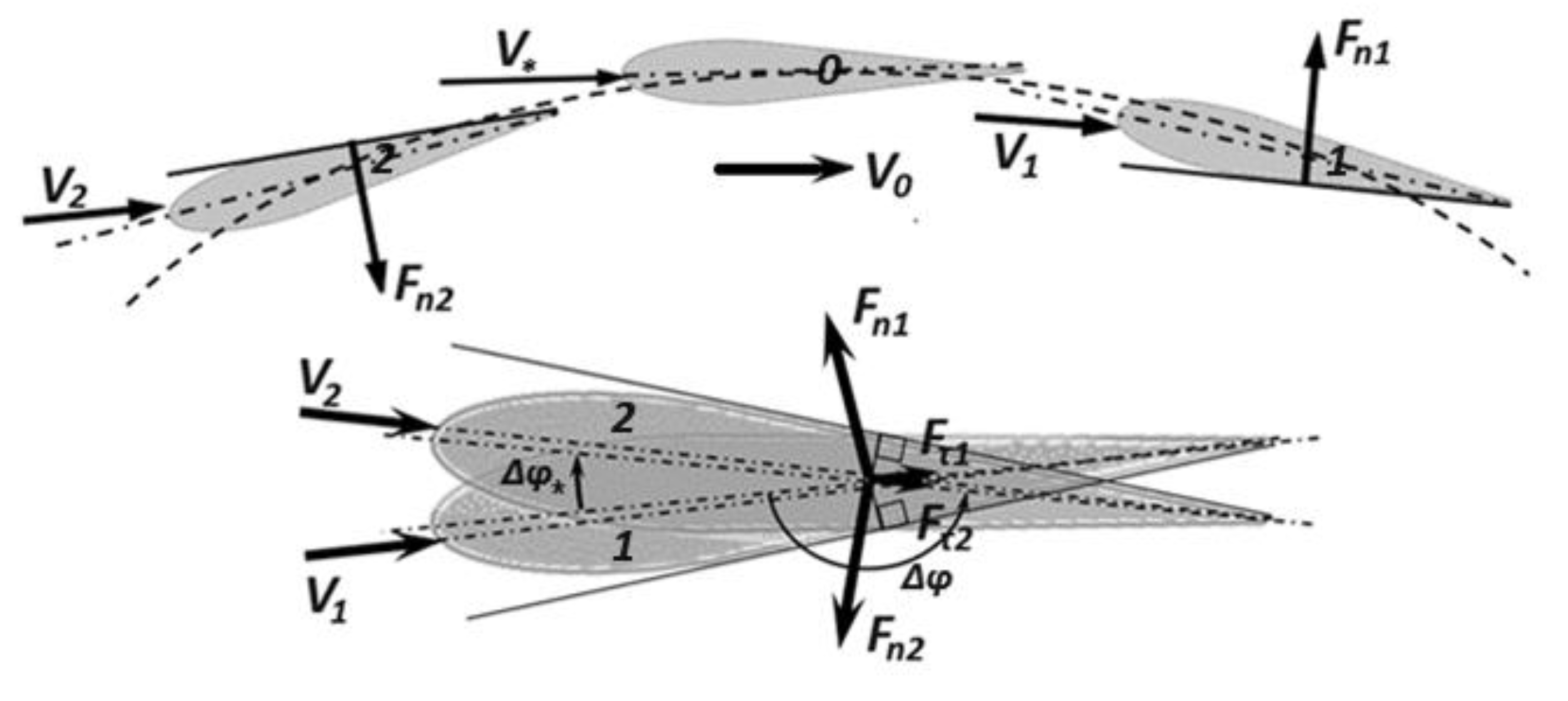
Figure 42.
An example of a comparative calculation of the distribution of blade orientation angles with direct inversion (solid line) and with reverse inversion (dashed line).
Figure 42.
An example of a comparative calculation of the distribution of blade orientation angles with direct inversion (solid line) and with reverse inversion (dashed line).
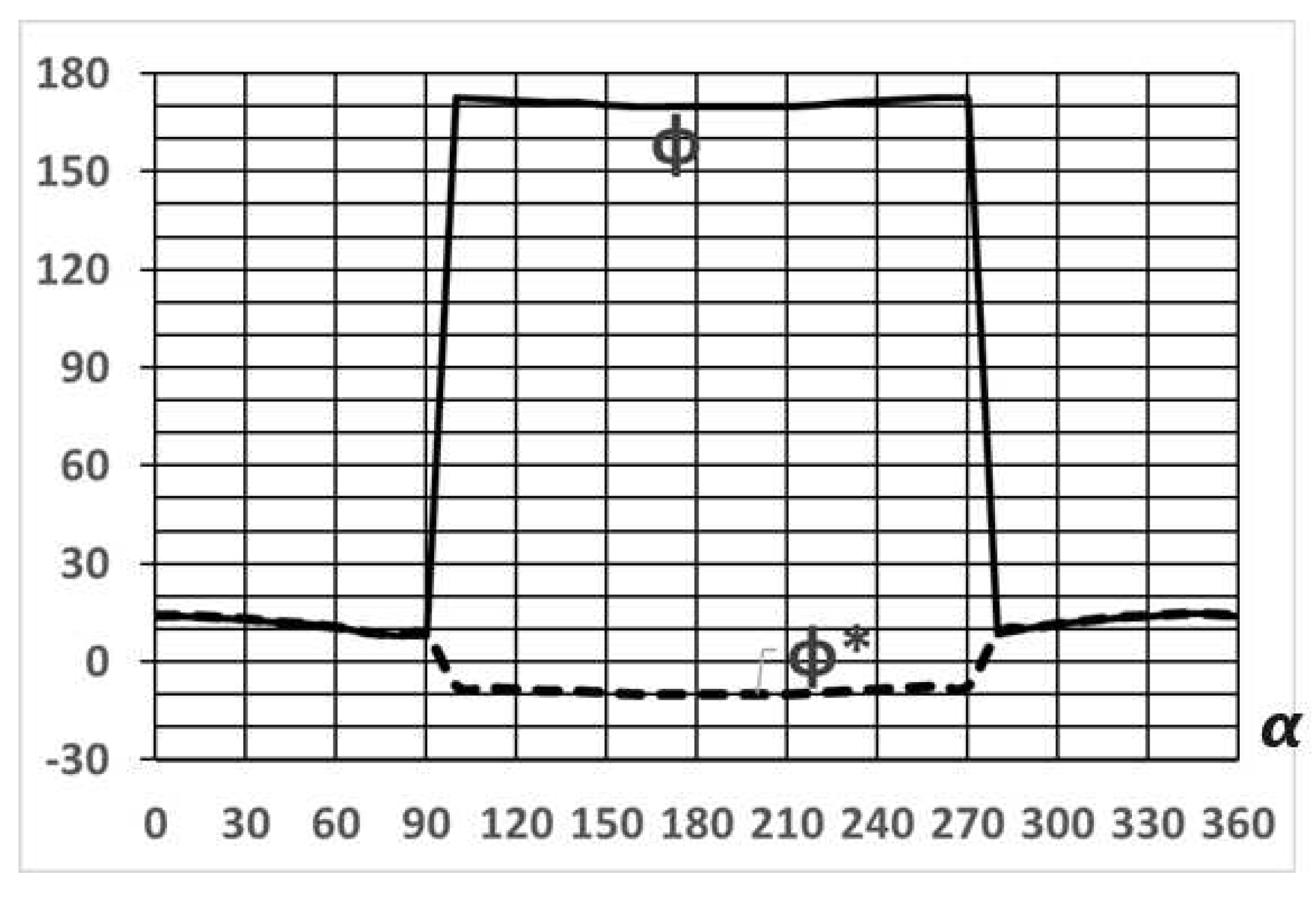
Figure 43.
An example of the dependence of the critical inversion angle from the opening angle of the symmetrical blade µ (angles in degrees).
Figure 43.
An example of the dependence of the critical inversion angle from the opening angle of the symmetrical blade µ (angles in degrees).
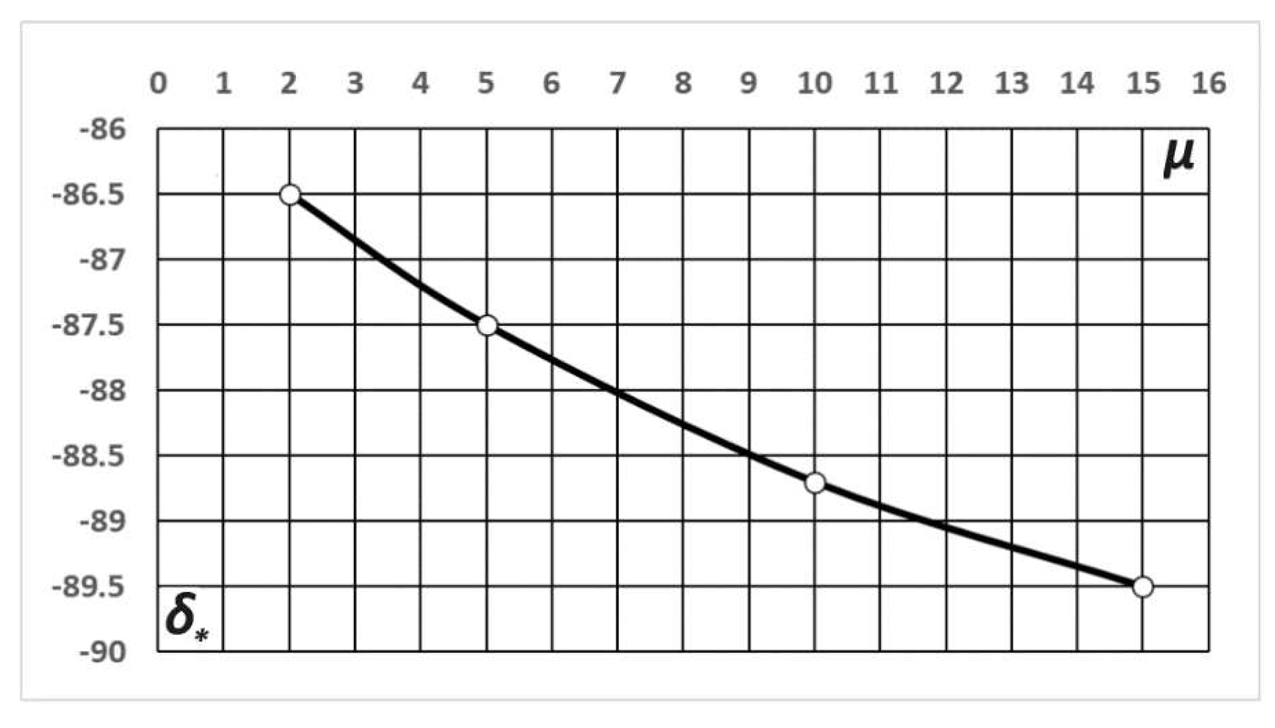
Figure 44.
Aerodynamic quasi-inversion mechanism symmetrical blade of a Darrieus turbine.
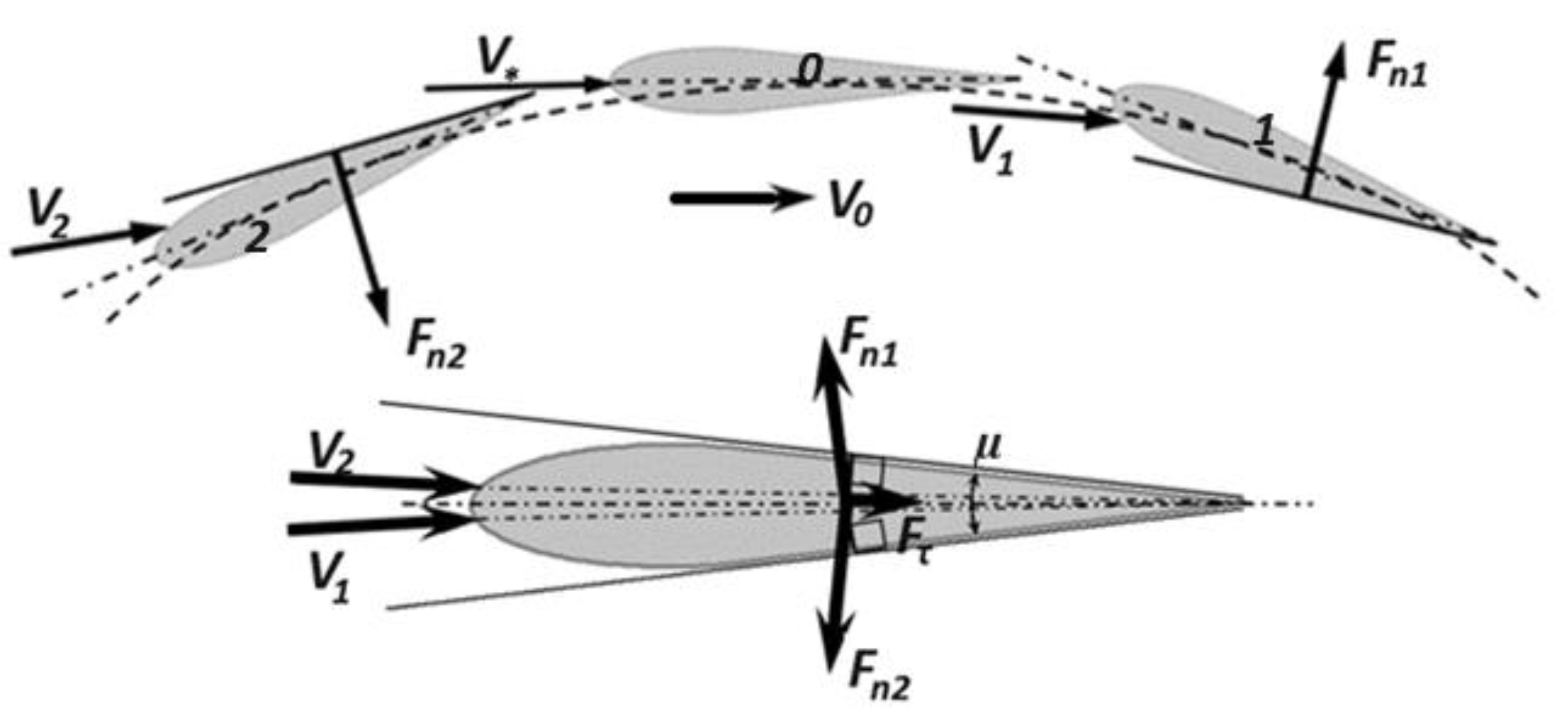
Figure 45.
An example of a comparative calculation of the distribution along the angular coordinate α of the relative flow direction angles δ, blade orientation φ* and angles of attack ψ. Parameter values: specific area of the blades Abi=0.1; speed index λ=4; blade opening angle µ=12o; a – adjustable symmetrical blades, b – Darrieus rotor.
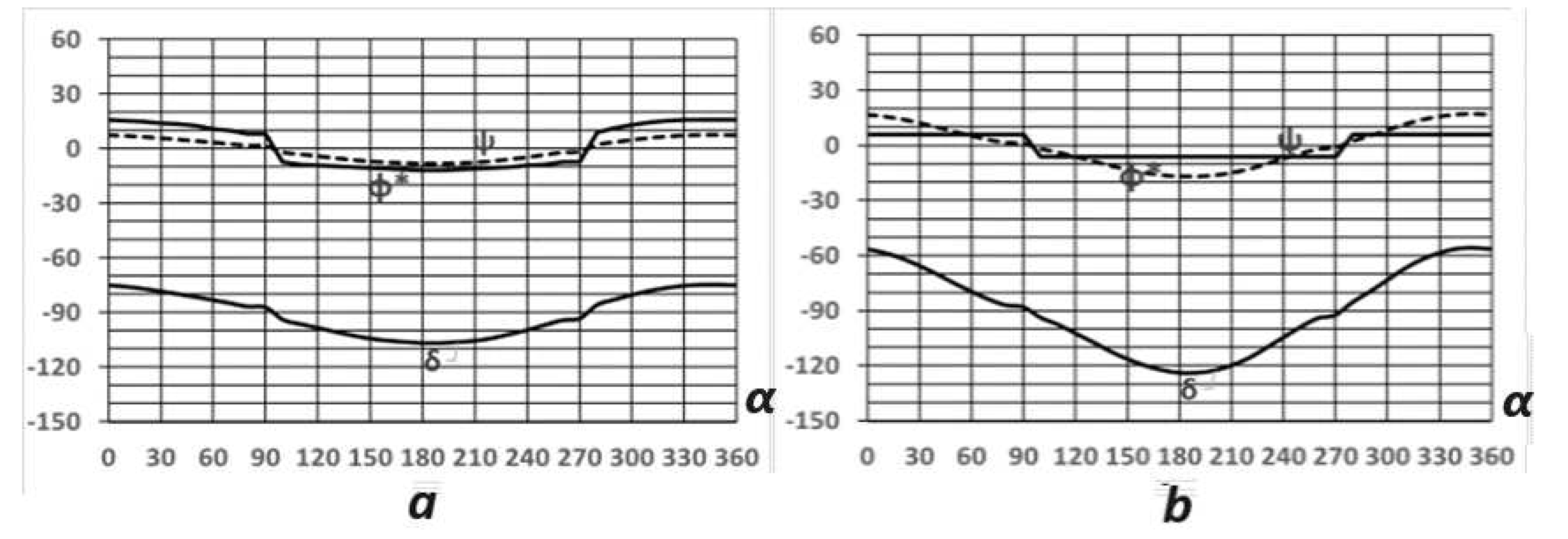
Figure 46.
Comparison of calculated and experimental dependences of power coefficients Ср on the speed index λ: 1 - experimental results [36] (Bravo et al. 2007) with amendments [37]; 2 - numerical results [31]; 3 - numerical results [37]; 4 - experimental results [36].
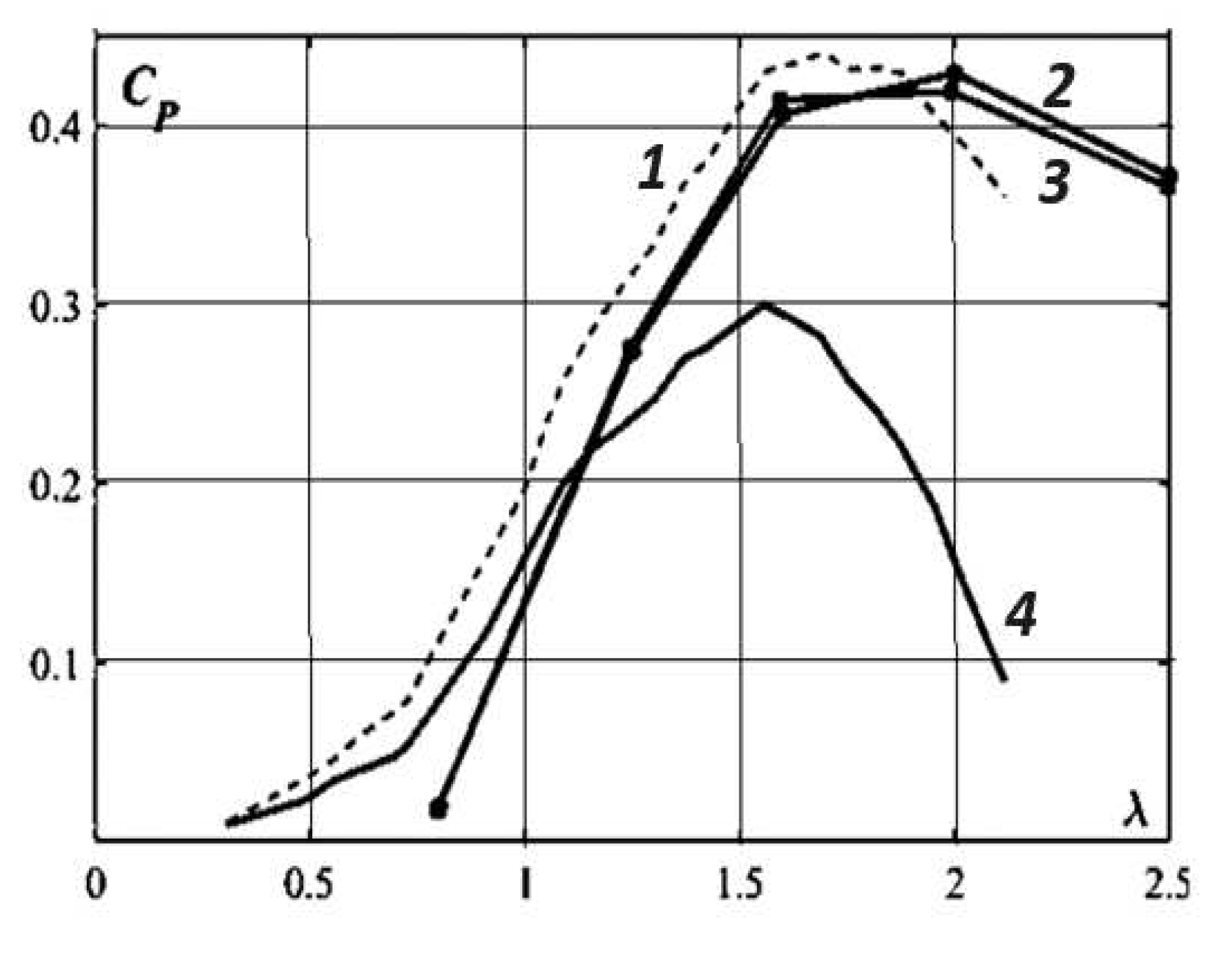
Figure 47.
Comparison of experimental and calculated results for an H-shaped turbine with a power of 200 W and, a rotate speed of 400 rpm, 1 – own calculated data; further source [21]: 2 - standard BEM curve; 3 - effects of the dynamic stall and flow curvature; 4 - passive torque effect; 5 – cumulative amendments; the points in the Figure represent experimental data.
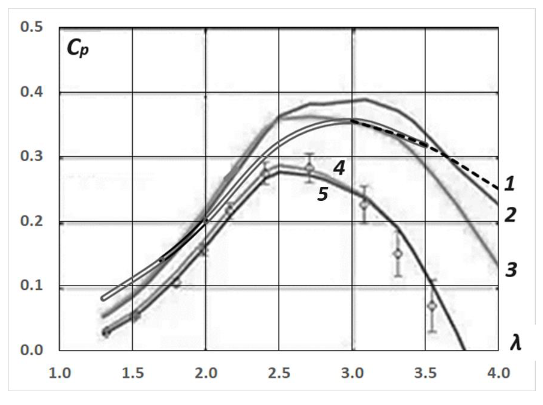
Figure 48.
The influence of the blade cross-section shape on distributed energy efficiency indicators. Blade opening angle, degrees – a) µ=5; b) µ =10; c) µ =15.
Figure 48.
The influence of the blade cross-section shape on distributed energy efficiency indicators. Blade opening angle, degrees – a) µ=5; b) µ =10; c) µ =15.
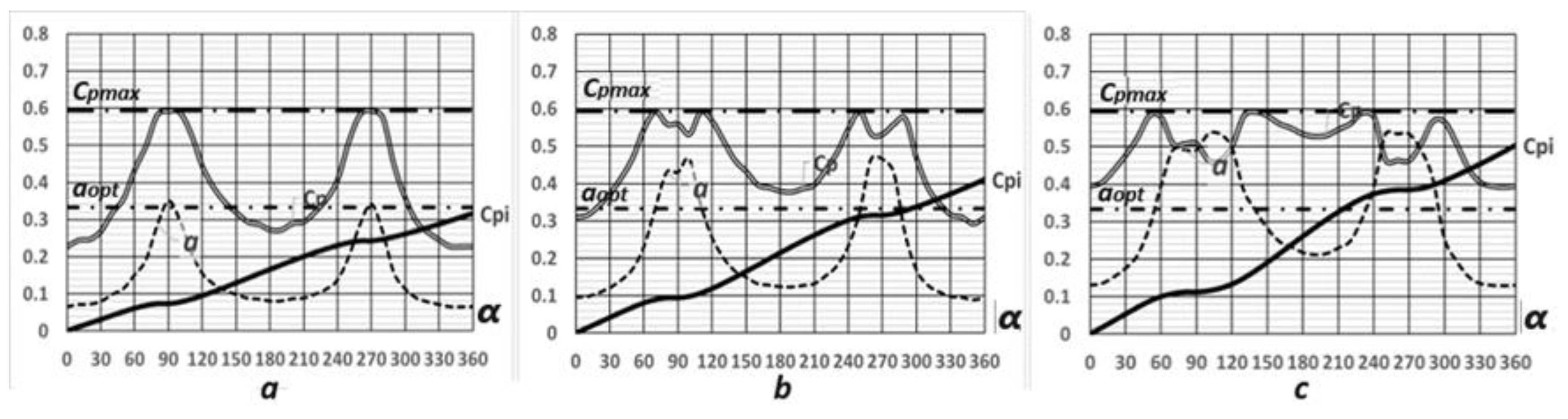
Figure 49.
The influence of the specific area of the blades on the distributed energy efficiency indicators: the total area of the blades divided by the area of the cylindrical surface of the turbine – а) =0.05; b) =0.10; c) =0.15.
Figure 49.
The influence of the specific area of the blades on the distributed energy efficiency indicators: the total area of the blades divided by the area of the cylindrical surface of the turbine – а) =0.05; b) =0.10; c) =0.15.
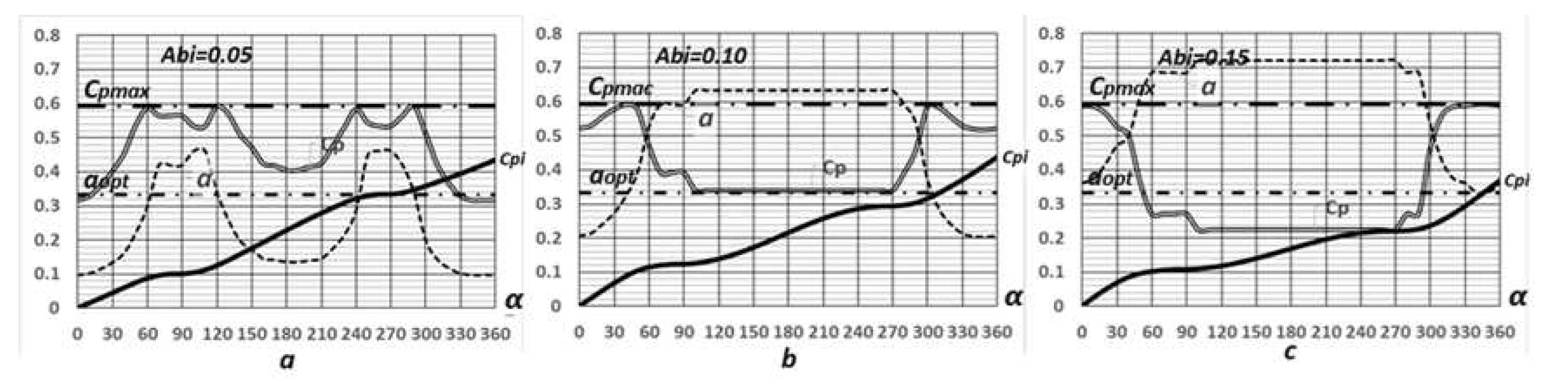
Figure 50.
The influence of turbine speed on distributed indicators energy efficiency: speed index - а) λ=2; b) λ=4; c) λ=6.
Figure 50.
The influence of turbine speed on distributed indicators energy efficiency: speed index - а) λ=2; b) λ=4; c) λ=6.
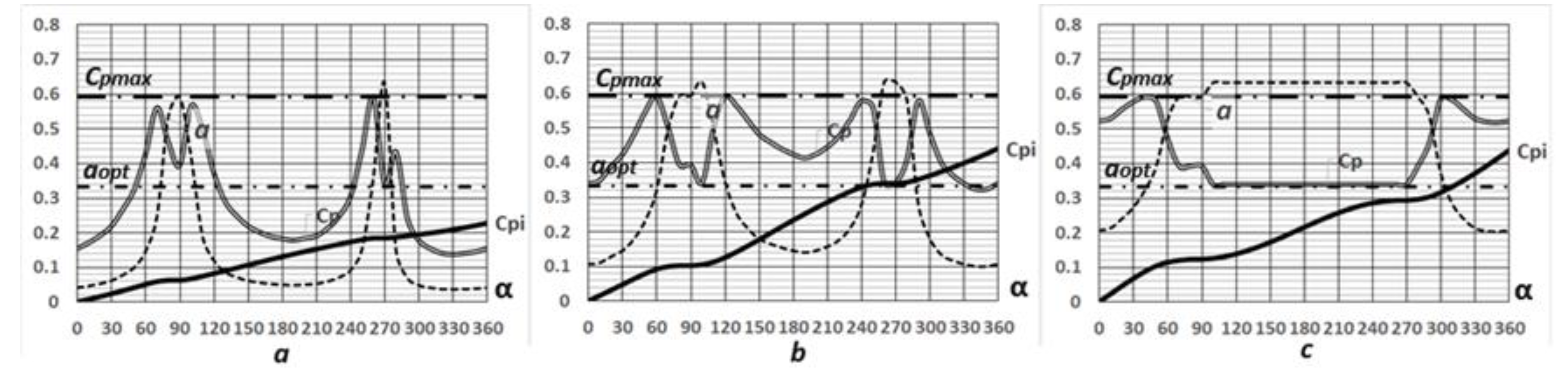
Figure 51.
Comparative distribution of calculated distributed indicators along the angular coordinate of an orthogonal turbine: speed index λ=5, opening angle of the blade section µ=12o, a - adjustable blades, b - Darrieus rotor.
Figure 51.
Comparative distribution of calculated distributed indicators along the angular coordinate of an orthogonal turbine: speed index λ=5, opening angle of the blade section µ=12o, a - adjustable blades, b - Darrieus rotor.
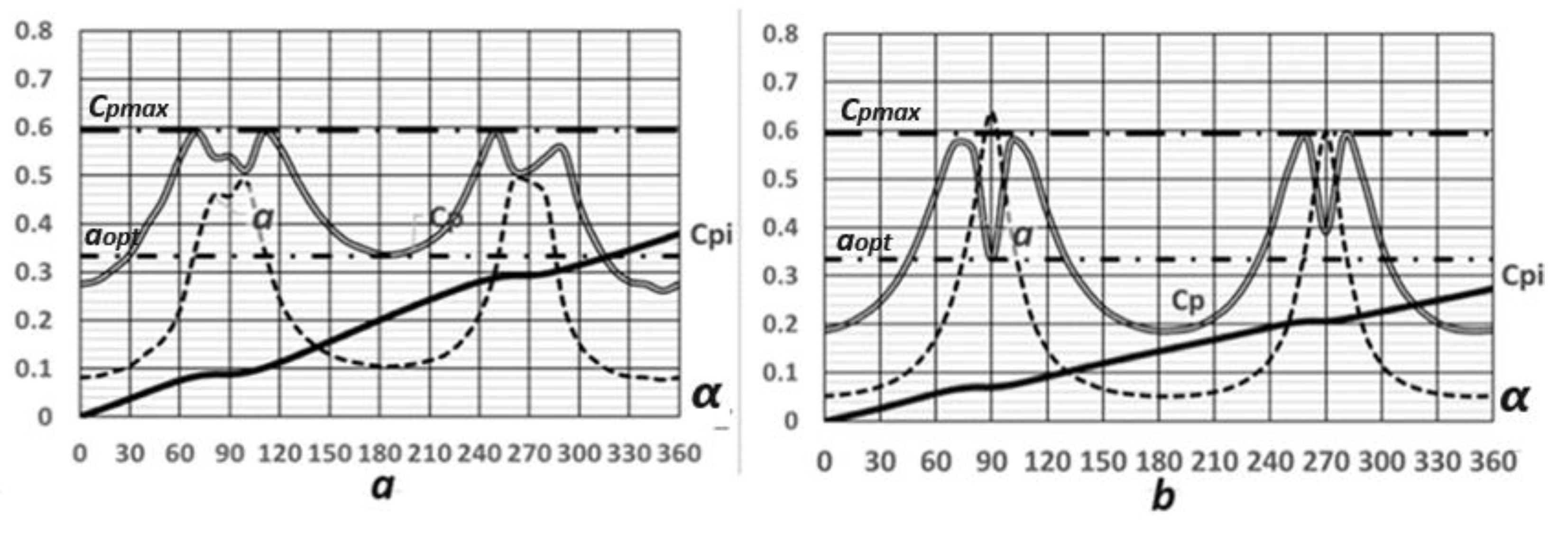
Figure 52.
Calculated dependences of power factors Ср orthogonal turbine on the speed index λ: line 1 – adjustable blades; line 2 – Darrieus rotor.
Figure 52.
Calculated dependences of power factors Ср orthogonal turbine on the speed index λ: line 1 – adjustable blades; line 2 – Darrieus rotor.
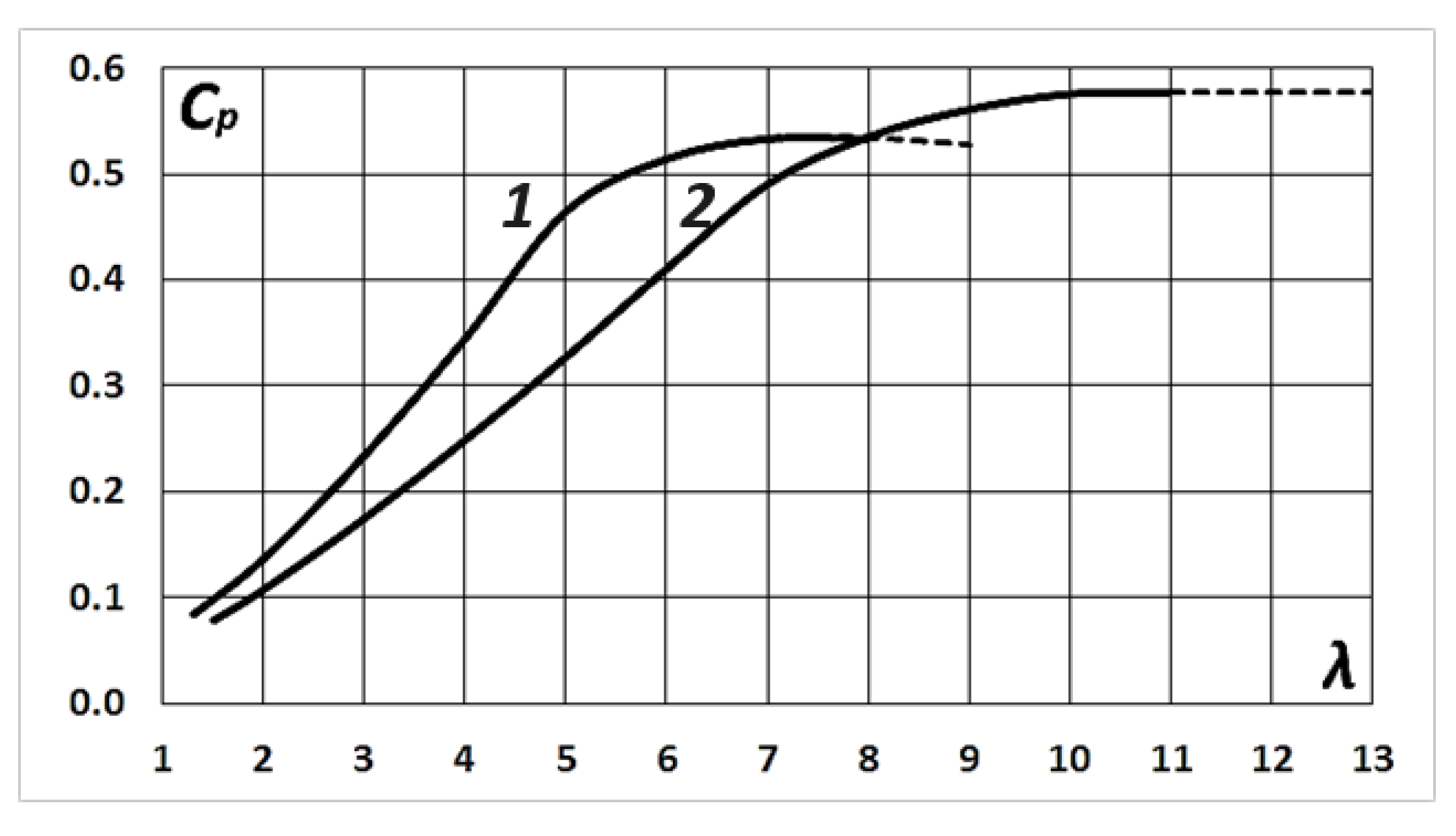
Figure 53.
Scheme of modification of a conventional turbine (a) into a multi-rotor turbine with quasi-translational movement of blades (b).
Figure 53.
Scheme of modification of a conventional turbine (a) into a multi-rotor turbine with quasi-translational movement of blades (b).
Figure 54.
Diagram of the interaction of air flow with a segment (local blade) of a collinear wind turbine: Ox – main turbine axis, Oz – reference axis of the blade, Z – reference coordinate segment, Ve is the portable velocity of the blade.
Figure 54.
Diagram of the interaction of air flow with a segment (local blade) of a collinear wind turbine: Ox – main turbine axis, Oz – reference axis of the blade, Z – reference coordinate segment, Ve is the portable velocity of the blade.
Figure 55.
Dependence of the optimal angular coordinate of the blade on the parameters of rotational speed, drag and lift force. Values for curves, respectively:1) 0; 2) 1.25; 3) 2.50; 4) 3.75.
Figure 55.
Dependence of the optimal angular coordinate of the blade on the parameters of rotational speed, drag and lift force. Values for curves, respectively:1) 0; 2) 1.25; 3) 2.50; 4) 3.75.
Figure 56.
Dependences of the extracted reduced flow power p on the parameters of the peripheral speed of the blade λ, drag s2 and lift force : a) ; b) ; c) . Curves 1, 2, 3, 4, 5, 6, 7, 8 correspond to the values - 0.35; 0.3; 0.25; 0.2; 0.15; 0.1; 0.05; 0.
Figure 56.
Dependences of the extracted reduced flow power p on the parameters of the peripheral speed of the blade λ, drag s2 and lift force : a) ; b) ; c) . Curves 1, 2, 3, 4, 5, 6, 7, 8 correspond to the values - 0.35; 0.3; 0.25; 0.2; 0.15; 0.1; 0.05; 0.
Figure 57.
Parametric dependencies for maximum characteristics “reduced power - peripheral speed parameter”: a) dependence of the maximum reduced power on the parameter lift force; b) dependence of the peripheral speed parameter at extreme points on the lift force parameter, Curves 1, 2, 3, 4, 5 correspond to the values of the drag parameter – 0.02; 0.04; 0.06; 0.08; 0.10.
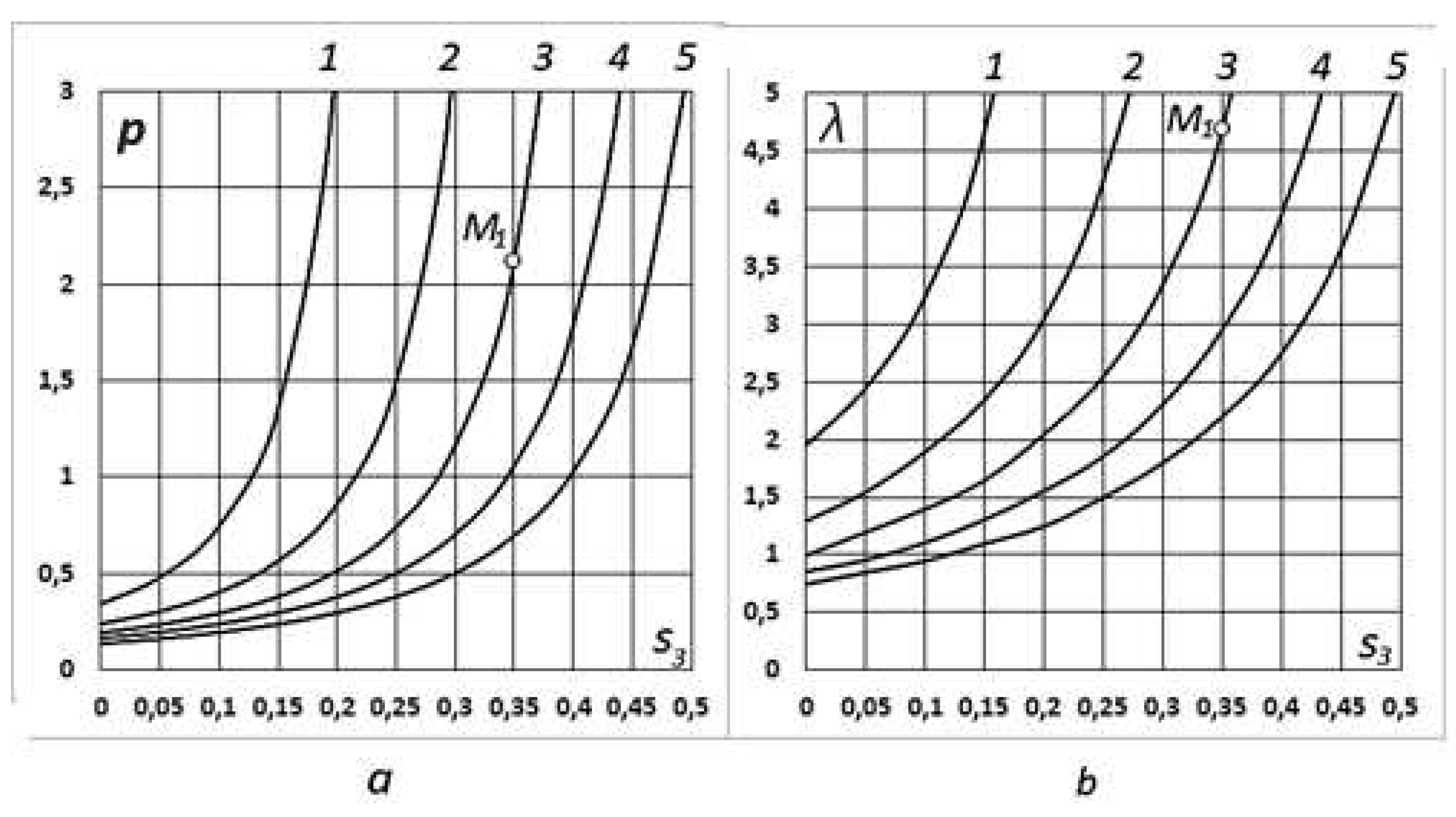
Figure 58.
Calculation diagrams of turbine rotor layout. Ratios of radii of levels: external (1), intermediate (2) and internal (3), respectively, 1: 2/3: 1/3.
Figure 58.
Calculation diagrams of turbine rotor layout. Ratios of radii of levels: external (1), intermediate (2) and internal (3), respectively, 1: 2/3: 1/3.
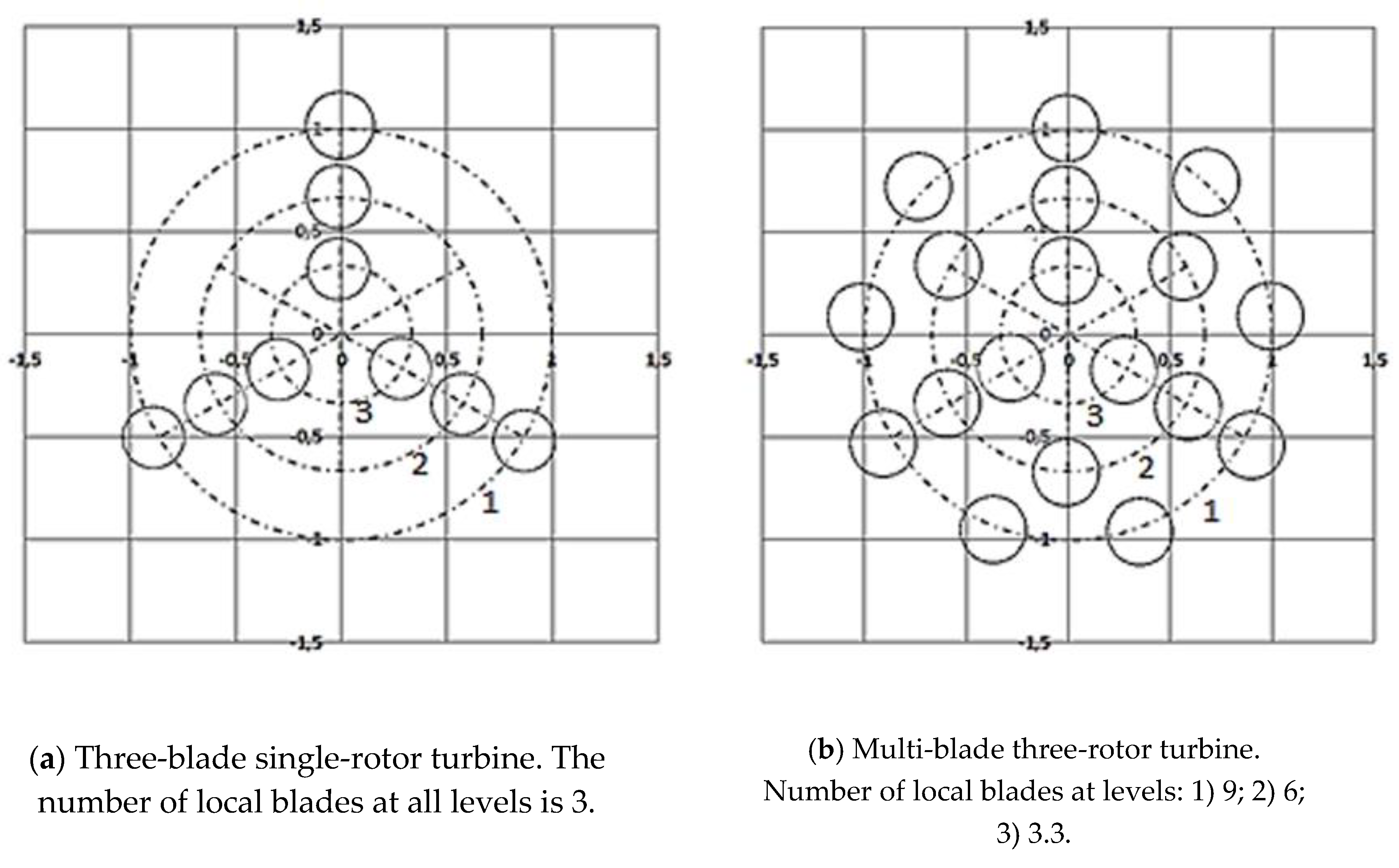
Figure 59.
Distributed geometric characteristics of the blades: a – conventional collinear turbine, blade shape factor n=-0.5; b – modified multi-rotor turbine, n=1.0; curves distributions: с – cumulative chord, σ – geometric density blades (dashed line); Аbi – integral specific area blades (thick line).
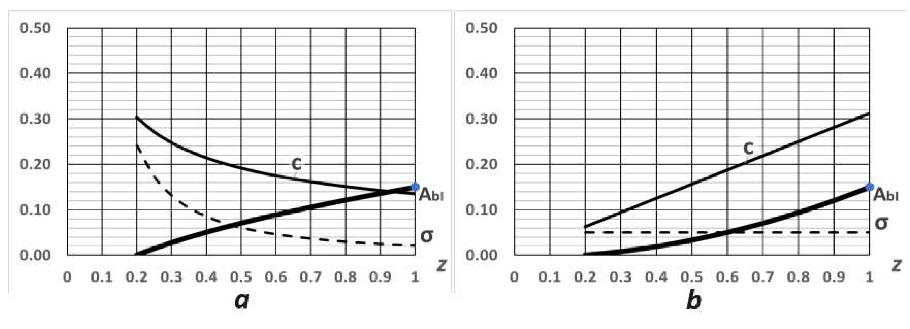
Figure 60.
Comparison of energy efficiency indicators conventional and modified turbines: a) conventional turbine, λ1=7; b) conventional turbine, λ1=4.2; c) modified turbine, λm =4.2.
Figure 60.
Comparison of energy efficiency indicators conventional and modified turbines: a) conventional turbine, λ1=7; b) conventional turbine, λ1=4.2; c) modified turbine, λm =4.2.
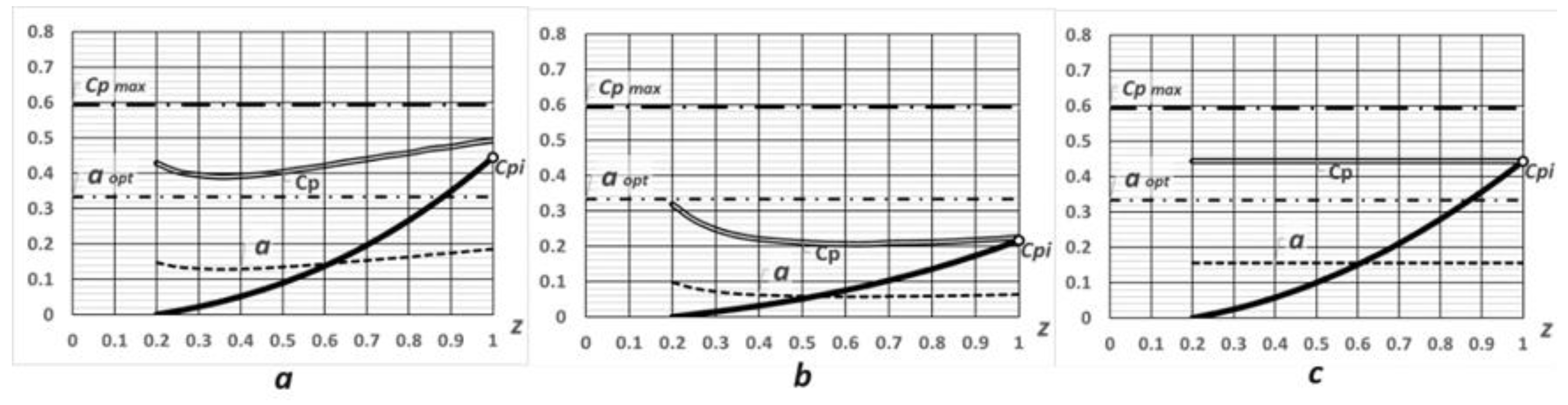
Figure 61.
Layout and design parameters of the turbine, dimensions in cm. R01, R1 - internal and external radii of the small rotor; R02, R2 are the corresponding radii of the large rotor. Selected areas of chord distribution: dark - chords of the blades; light ones - cumulative chords.
Figure 61.
Layout and design parameters of the turbine, dimensions in cm. R01, R1 - internal and external radii of the small rotor; R02, R2 are the corresponding radii of the large rotor. Selected areas of chord distribution: dark - chords of the blades; light ones - cumulative chords.
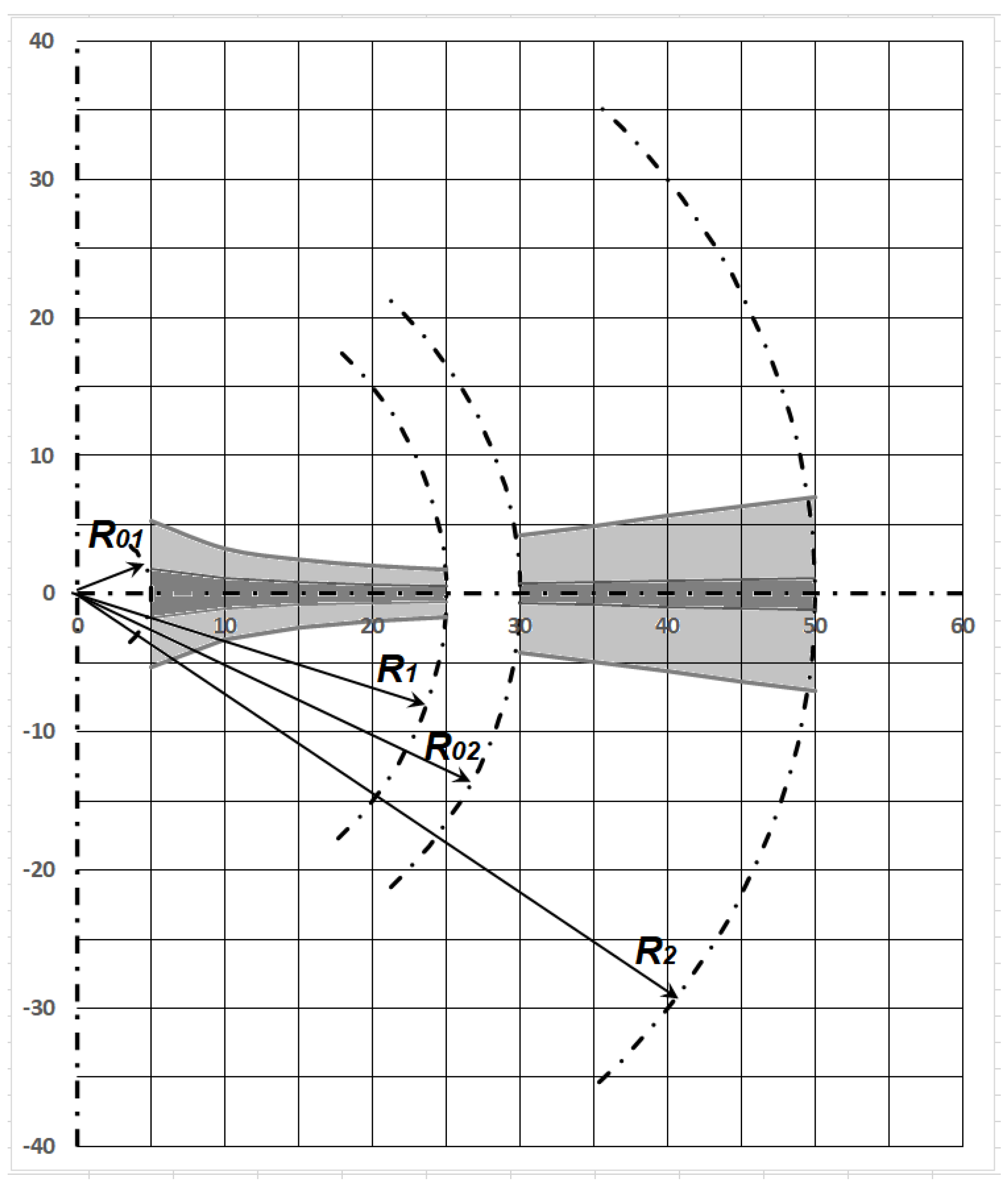
Figure 62.
Distribution of total chords along the length of the blades, see: 1 - small rotor; 2 – large rotor.
Figure 62.
Distribution of total chords along the length of the blades, see: 1 - small rotor; 2 – large rotor.
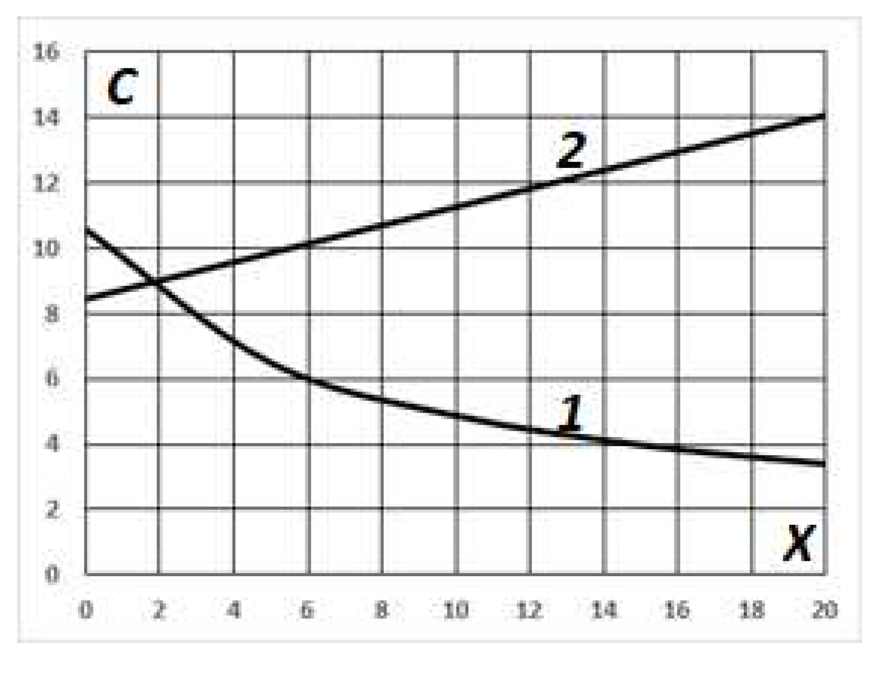
Figure 63.
Distribution of twist angles along the length of the blades, degrees: 1 - small rotor; 2 – large rotor.
Figure 63.
Distribution of twist angles along the length of the blades, degrees: 1 - small rotor; 2 – large rotor.
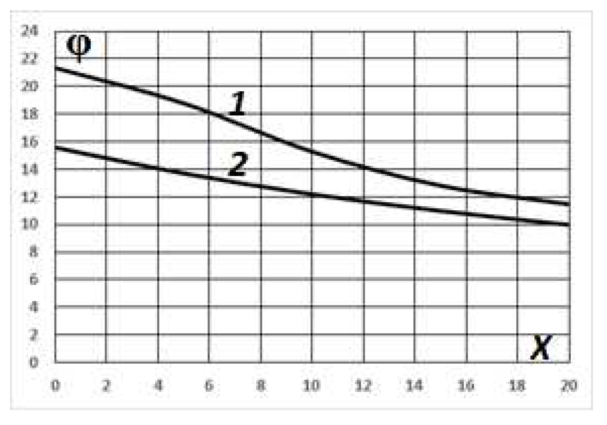
Figure 64.
Formation of the basic profile of the blades.
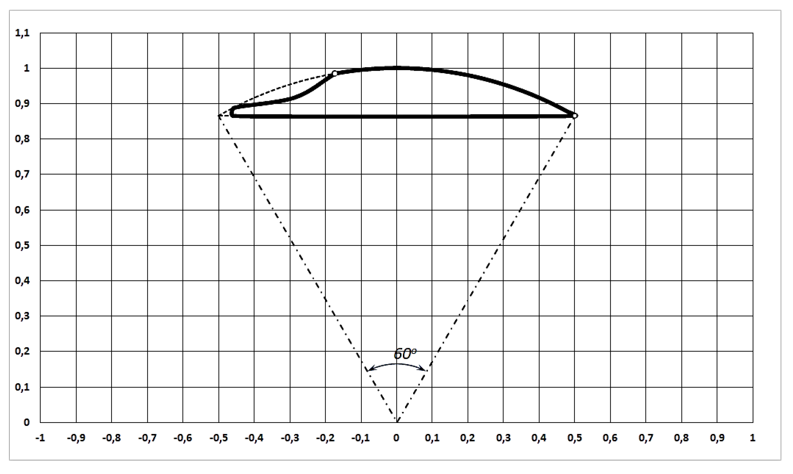
Figure 65.
Varying the blade profile.
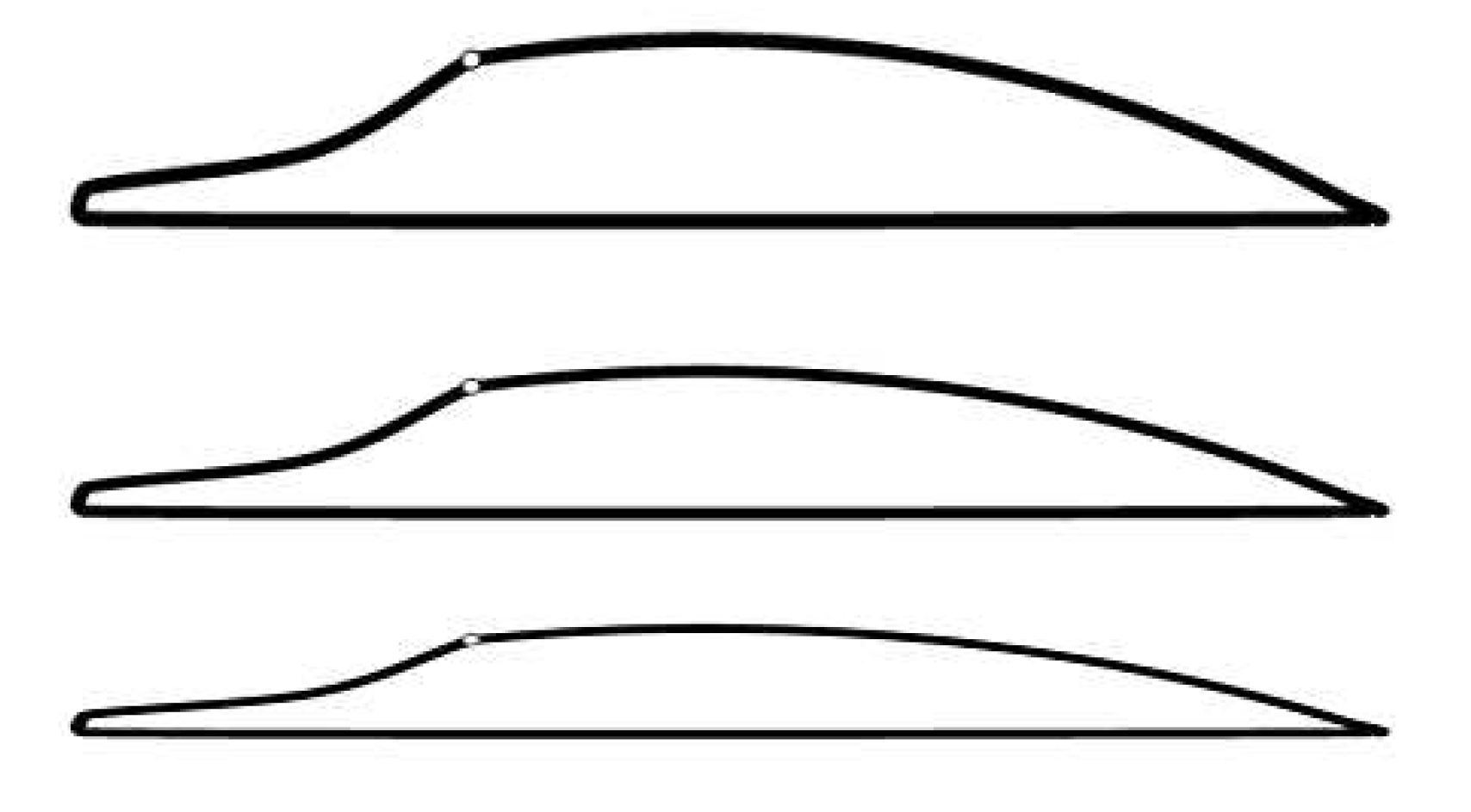
Table 1.
Turbine ERDA–NASA MOD-0: initial data.
| Rotor diameter, m | D | 38 |
|---|---|---|
| Rotor speed, rpm | ν | 40 |
| Wind speed, m/s | V0 | 8 |
| Angle of attack, degrees | α | 8 |
| Number of blades | B | 2 |
| Number of calc. steps | K | 20 |
Table 2.
Comparative calculation. Summary data.
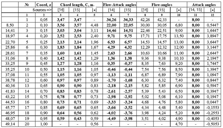 |
Table 3.
Power factors by source.
| [14] | Wilson, R.E. et al. 1976 | Cpi | 0.547 | Title 3 |
| [15] | Maalawi, K.Y. et al. 2001 | 0.531 | data | |
| [*] | Proposed technique | 0.553 | data 1 |
Table 4.
NREL Wind Turbine Specifications.
| Parameters | Units | Values |
|---|---|---|
| Rotor diameter | m | 10.6 |
| Rotation speed | rpm | 72 |
| Rated power | kW | 10 |
| Blade pitch angle | degree | 3 |
| Number of blades | - | 2 |
| Blade profile | - | S809 |
Table 5.
Energy parameters of segments of a conventional three-blade turbine.
| N1 | N2 | N3 | |
|---|---|---|---|
| λ | 4.65 | 3.10 | 1.55 |
| p | 2.12 | 1.67 | 0.80 |
Table 7.
Distribution of blade twist angles.
| X, sm. | 0 | 2.5 | 5 | 7.5 | 10 | 12.5 | 15 | 17.5 | 20 |
|---|---|---|---|---|---|---|---|---|---|
| φ1, deg. | 21.31 | 20.71 | 18.76 | 16.86 | 15.26 | 13.91 | 12.81 | 11.86 | 11.11 |
| φ2, deg. | 15.56 | 14.56 | 13.71 | 12.91 | 12.21 | 11.61 | 11.01 | 10.46 | 10.01 |
Disclaimer/Publisher’s Note: The statements, opinions and data contained in all publications are solely those of the individual author(s) and contributor(s) and not of MDPI and/or the editor(s). MDPI and/or the editor(s) disclaim responsibility for any injury to people or property resulting from any ideas, methods, instructions or products referred to in the content. |
© 2024 by the authors. Licensee MDPI, Basel, Switzerland. This article is an open access article distributed under the terms and conditions of the Creative Commons Attribution (CC BY) license (http://creativecommons.org/licenses/by/4.0/).
Copyright: This open access article is published under a Creative Commons CC BY 4.0 license, which permit the free download, distribution, and reuse, provided that the author and preprint are cited in any reuse.


