
Submitted:
22 December 2023
Posted:
25 December 2023
You are already at the latest version
Abstract
An integrated approach to active flow control is proposed by finding both the drooping leading edge and the morphing trailing edge for flow management. This strategy aims to manage flow separation control by utilizing the synergistic effects of both control mechanisms, which we call the Combined Morphing Leading Edge and Trailing Edge (CoMpLETE) technique. This design is inspired by a bionic porpoise nose and the flap movements of the cetacean species. The motion of this mechanism achieves a continuous, wave-like, variable airfoil camber. The dynamic motion of the airfoil's upper and lower surface coordinates in response to unsteady conditions is achieved by combining the thickness-to-chord (t/c) distribution with the time-dependent camber line equation. A parameterization model was constructed to mimic the motion around the morphing airfoil at various deflection amplitudes at stall angle of attack and morphing actuation start times. The mean properties and qualitative trends of the flow phenomena are captured by the transition-SST (Shear Stress Transport) model. The effectiveness of the dynamically morphing airfoil as a flow control approach is evaluated by obtaining the flow field data, such as velocity streamlines, vorticity contours, and aerodynamic forces. Different cases are investigated for the CoMpLETE morphing airfoil, which evaluates the airfoil’s parameters, such as its morphing location, deflection amplitude, and morphing starting time. The morphing airfoil’s performance is analyzed to provide further insights into the dynamic lift and drag force variations at pre-defined deflection frequencies of 0.5 Hz, 1 Hz, and 2 Hz. The findings demonstrate that adjusting the airfoil camber reduces streamwise adverse pressure gradients, thus preventing significant flow separation. Although the trailing edge deflection and its location along the chord influence the generation and separation of the Leading-Edge Vortex (LEV), these results show that the combined effect of the morphing leading edge and trailing edge has the potential to mitigate flow separation. The morphing airfoil successfully contributes to the flow reattachment and significantly increases the maximum lift coefficient (c_(l,max))). This work also broadens its focus to investigate the aerodynamic effects of a dynamically morphing leading and trailing edge, which seamlessly transitions along the side edges. The aerodynamic performance analysis is investigated across varying morphing frequencies, amplitudes, and actuation times.
Keywords:
Morphing
; Unsteady Parameterization
; Combined Morphing Leading Edge and Trailing Edge (CoMpLETE)
; Flow Control
1. Introduction
The increased demand for air travel has generated environmental concerns and significantly impacted the aircraft industry. The aviation sector aims for net-zero carbon emissions by 2050. To reduce CO2 emissions, the UN's International Civil Aviation Organization (ICAO) organized negotiations and has given recommendations that include increasing aircraft innovation and “streamlining” flying operations. The aviation sector's main objectives encompass enhancing air travel quality and affordability, reducing CO2, NOX, and noise emissions, and addressing safety concerns [1]. These challenges have spurred a greater need for innovative research to develop more efficient and environmentally friendly aircraft. The Research Laboratory in Active Controls, Avionics, and AeroServoElasticity (LARCASE) has continued to explore numerous strategies to reduce aircraft fuel consumption and emissions [2,3,4,5,6,7,8].
Advanced aerodynamic design technologies will play a crucial role in improving next-generation aircraft performance, reliability, and maneuverability. Flow separation control studies are critical to the aircraft industry [9]. At low Reynolds numbers, a laminar boundary layer forms on an airfoil's upper (suction) surface, which is prone to separate with or without turbulent flow reattachment, depending on the angle of attack. When the angle of attack increases towards the stall angle of the airfoil, the adverse pressure gradient on the suction side increases. The flow separation point moves upstream and is displaced towards the leading edge. The adverse pressure gradient continues to increase to a certain point, at which the flow boundary layer separates near the leading edge on the suction side. As the angle of attack value attains the stall angle, the lift coefficient increases until it reaches the maximum lift coefficient. From that point, there is a significant drop in the airfoil lift and stall phenomena.
Various active and passive flow control technologies have been developed and applied in diverse practical applications [10,11,12,13,14,15,16]. Morphing technology can enhance an aircraft's performance using various parameters, including lift, drag, and flow separation control [17,18,19,20,21]. During flight, mission requirements frequently change, and aircraft often operate in less-than-ideal conditions. In terms of aerodynamics, conventional aircraft employ hinged mechanisms for high-lift systems and trailing edge surfaces to control the airflow. However, these mechanisms can also lead to increased drag [22]. These hinged surfaces have limitations when deployed and retracted [23]. Improper alignment of high-lift surfaces can generate noise and turbulence, resulting in flow separation.
Leading-edge morphing control is a widespread technique that facilitates alterations in wing curvature. The control of Leading-Edge Vortices (LEVs) is achieved through active or passive modifications of the leading-edge shapes. The aerodynamic characteristic of the wavy leading-edge results in a gradual stall behavior characterized by a smooth reduction in lift rather than an abrupt loss. The concept of variable-droop leading edge (VDLE) control involves the downward morphing of a specific section of the leading edge, wherein the morphing angle varies with time [24].
The Variable Droop Leading Edge (VDLE) design has demonstrated that the local angle of attack near it reduces when the overall angle of attack exceeds a certain threshold [24]. Consequently, this reduction mitigates the adverse pressure gradient, thus minimizing the leading-edge vortex formation and the occurrence of flow separation and dynamic stall.
An investigation was conducted on implementing a combined leading-edge droop and Gurney flap to enhance the aerodynamic properties of both dynamic stall and post-stall in a rotor airfoil [25]. The experimental findings indicated that the onset of dynamic stall was delayed by 20 degrees when a leading-edge droop of 20 degrees and a Gurney flap with a chord length of 0.5% were employed. Another study employed VDLE using computational methods; their findings revealed a significant decrease in the drag and moment rise typically associated with dynamic stall [26].
However, it was also demonstrated that the drooped leading-edge system could not achieve the necessary lift and stall performance at high angles of attack compared to the advantages offered by a multi-element, typical high-lift system consisting of a slat and slot [27].
The aerodynamic performance of a morphing airfoil and wing with LE and TE parabolic flaps was quantitatively evaluated and further compared to prove its efficacy [28]. That work thoroughly analyzed airfoil aerodynamics using four typical design parameters. Parabolic flaps outperformed articulated flaps for airfoil lift increase with 39.2% and drag reduction of 108.4%, enhancing aerodynamic efficiency, respectively.
Variable-Camber Continuous Trailing-Edge Flap (VCCTEF) technology was developed for a NASA general transport aircraft to study the drag reduction effect of the morphing TE [29], thus achieving an 8.4% drag reduction. Deflection frequency and angle effects were analyzed in a morphing LE airfoil’s aerodynamics under steady and unsteady conditions [30]. The impact of Trailing Edge Flaps (TEF) on mitigating both the negative pitching moment and aerodynamic damping induced by a Dynamic Stall Vortex (DSV) was examined in [31]. The authors have explained these negative effects were linked to the trailing edge vortex. Gerontakos and Lee conducted wind tunnel test studies to investigate the impact of TEF deflections on the dynamic loads generated by an oscillating airfoil motion [32]. The tests considered various parameters, such as the flap actuation start times, durations, and amplitudes. Interestingly, the results indicated that TEF's motion did not affect the separation of the DSV. However, the duration of TEF deflection has impacted the airfoil's maximum lift.
Unsteady flow characteristics and responses of a morphing airfoil under near-stall conditions were evaluated, and it was shown that a downward TE might increase lift instantly [33,34]. They analyzed the unstable aerodynamics of a morphing wing with a smooth side-edge transition [35]. Their results showed that the dynamically morphing wing's unsteady flow impact might cause a substantial initial drag coefficient overshoot proportionally related to the morphing frequency.
One approach to control dynamic stall involves using a leading-edge slat device, which was analyzed through numerical simulations using a two-dimensional Navier–Stokes solver for multi-element airfoils [36]. Another option consists of employing suction or blowing techniques. An experiment for dynamic-stall control was conducted using blowing slots positioned at 10% and 70% of the airfoil chord length [37].
One study demonstrated that the utilization of a small leading edge angle (10°) morphing technique for a high angle of attack (> 25°) leads to a notable enhancement in the efficiency of propulsion compared to that achieved with a rigid airfoil [38]. The work shown in [39] has demonstrated that the objective function determines the ideal suction speed. The approach involves modifying the airfoil's geometry, and the airfoil's nose radius was gradually adjusted to delay flow separation. At the same time, [40] used the nose droop of the VR-12 airfoil, setting the rotation angle at 25% of the chord and the droop angle at 13 degrees.
The potential of combustion-powered actuation to suppress dynamic stall on a high-lift rotorcraft airfoil was explored in [41]. Particle Image Velocimetry was employed to investigate the flow mechanisms involved in stall suppression. The test results indicated that combustion-powered actuators could significantly enhance the airfoil's stall behavior at Mach number values up to 0.4. At Mach number 0.4, the cycle-averaged lift coefficient increased by 11% during the dynamic stall process. An investigation into the impact of a co-flow jet on the dynamic stall of a wind turbine airfoil was presented in [42]. The results showed that dynamic stall could be significantly reduced, and energy consumption research revealed that the co-flow jet concept effectively controlled the dynamic stall.
Another study demonstrated that the transient lift coefficient associated with Leading Edge (LE) morphing during the nose-up phase had a greater magnitude than that observed in the static situation [30]. The primary objective of the TE control is to enhance the moment characteristics and mitigate the dynamic stall compared to that achieved with conventional rudder surfaces. Performance enhancement techniques, such as Trailing Edge (TE) morphing [43,44] can be employed. Combined LE–TE control integrates the characteristics of both LE and TE controls, such as the combination of LE droop, resulting in an enhanced suppression stall effect [44].
Another study explored the impact of a trailing-edge flap on dynamic stall effects at high speeds in wind turbines [45]. The pitching of the trailing edge flap influences the dynamic stall hysteresis loops, which leads to load fluctuations. The consideration of the trailing edge flap reduced the cyclic variability in the lift coefficient and the root bending moment by a minimum of 26% and 24%, respectively. These findings provide valuable insights into the advantages of trailing edge flaps and their potential to mitigate load variations in wind turbine blades.
A numerical investigation focused on the blade section of a helicopter rotor during forward flight aimed to reduce or alleviate dynamic stall on the retreating blade [46]. For validation and verification purposes, simulations were conducted for flows around static and pitching airfoils at constant and variable Mach numbers. Their results were compared with other numerical data and experimental findings. Notably, the maximum drag coefficient () and the absolute value of the minimum pitching moment coefficient () were reduced by up to 49.2% and 25%, respectively. It is worth noting that the dynamic stall was eliminated using the proposed airfoil deformation under certain flow conditions.
The analysis focused on the leading-edge alteration inspired by cetacean species, specifically the porpoise [47]. This modification was applied to multiple airfoils, and the analysis was conducted at varied speeds. A three-dimensional numerical analysis was conducted on the impact of the spanwise placement and the extent of leading-edge alterations. The design of the porpoise nose, characterized by its shorter length and medium depth, has delayed flow separation and enhanced aerodynamic efficiency up to the crucial Mach number.
Recognizing the potential of both the drooping leading edge and the morphing trailing edge in flow control, this paper suggests an integrated approach to active control. This approach, called the Combined Morphing Leading Edge and Trailing Edge (CoMpLETE), seeks to harness the complementary effects of both control mechanisms to manage flow separation control effectively. Understanding the turbulent flow phenomena characterizing this approach will be valuable. Only a few articles in the literature thoroughly explore the CoMpLETE concept and its various parameters, including deflection frequency and extent and the starting morphing time.
The paper also expands its scope to explore the unsteady aerodynamic consequences of applying CoMpLETE to an airfoil with a seamless flow transition. The study includes an aerodynamic performance analysis at different morphing frequencies, amplitudes, and actuation times. The objective is to understand how these diverse morphing frequencies affect the wing's aerodynamic behavior and its overall performance.
2. Morphing Model
The current research proposes to exploit the complementary effects of both leading edge and trailing edge control mechanisms to effectively manage flow separation control of an airfoil, using an approach called CoMpLETE (Combined Morphing Leading Edge and Trailing Edge). This design is inspired by a bionic porpoise nose and flap motions of the cetacean species. The motion of this mechanism achieves a continuous, wave-like, variable camber. The dynamic motion of the airfoil's upper and lower surface coordinates in response to unsteady conditions is achieved by combining the thickness distribution with the time-dependent camber line equation. Additionally, the motion of the airfoil's deflection is designed to start from its baseline configuration, progress to achieve a maximum downward target position, return to the original baseline configuration, and follow a sinusoidal pattern. Figure 1 depicts the model of various motions in cetacean species; it is evident that the mechanism undergoes slight oscillations, and similar airfoil motions can be obtained and investigated.
To obtain a fully dynamically morphing airfoil, precise definitions are essential for the changing shapes of the leading and trailing edges and their dynamic deformations. These definitions rely on a parametric approach that accurately represents the airfoil's boundary and geometry. Incorporating control parameters derived from the 4-digit NACA airfoil made it possible to dynamically modify the curvature of the camber line within the morphing section of the airfoil's chord. This innovation allowed the design of a novel airfoil shape incorporating time-varying elements into the parametric equations governing the trailing edge geometry.
Because of the inherent asymmetry of the UAS-S45 airfoil, it was not feasible to directly apply or convert the mathematical model designed for symmetric airfoils. Consequently, a distinct approach was developed, explicitly tailored for asymmetric airfoils. In this context, the curvature and type of an asymmetric airfoil are determined by its camber. Figure 2 provides an illustration of the essential parameters considered within the model for morphing the leading edge, where P is the point where morphing starts.
The dynamic motion of the airfoil's upper and lower surface coordinates in response to unsteady conditions is achieved by combining the thickness distribution with the time-dependent camber line equation. Additionally, the motion of the airfoil's deflection is initiated from its baseline configuration, progresses to achieve a maximum downward target position, returns to its baseline configuration, and follows a sinusoidal pattern. The parametrized time-dependent camber line is defined by the following equation:
where t is the time variable, and f is the airfoil deflection frequency (cycles per second). Five main parameters were determined to be of crucial importance for the airfoil morphing control: M, P, , and . Figure 3 depicts some of these parameters.
This research investigates the impact of this morphing approach on the flow separation occurring on the UAS-S45 airfoil. The study elucidates how the airfoil's upward and downward deflections influence the separation bubble's development during the airfoil's oscillating motion.
Different cases were set up with different morphing motions (synchronous and asynchronous) based on the morphing approach. Different morphing starting times and deflection frequencies were used to obtain different morphing shapes at different time steps. Two major studies were carried out based on the morphing airfoil chord location. In Table 1, the morphing of the leading edge starts at 0.2c, and the trailing edge morphing starts at 0.75c; in Table 2, the morphing of the leading edge starts at 0.15c, and the trailing edge morphing starts at 0.75c. The flow behavior was then analyzed for these cases, as shown in Table 1 and Table 2.
2.2. Computational Domain and Grid Definitions
The size and configuration of the computational domain significantly impact the accuracy of results, especially concerning the aerodynamics of the geometry in question. In this particular aerodynamic scenario, the 2D computational domain forms a C-shaped grid, extending 20 times the airfoil chord length upstream (20c) and 30 times downstream (30c). These dimensions have been chosen to obtain a balance: the inlet and outlet distances are sufficiently large to ensure that the boundary conditions at the outer domain do not interfere with the airfoil's flow, yet small enough to maintain reasonable computational efficiency.
This study used hybrid mesh, as depicted in Figure 4. These meshes combine structured quadrilateral layers near the airfoil with unstructured triangular elements elsewhere. Employing a blunt trailing edge makes it possible to design smoothly transitioning O-shaped block layers surrounding the airfoil, thereby reducing instabilities that could arise from sharp corners at the trailing edge.
The wall condition parameter, denoted as , serves as a dimensionless measure of the distance from the wall to the first grid point and is critical for assessing the "near-wall" mesh requirements. To accurately capture the characteristics of the near-wall region, a grid that aligns with the requirements of a chosen turbulence model is established. In this investigation, the turbulence model requires that the first cells near the airfoil should be positioned within the viscous sublayer, aiming for a value of less than one, that is recommended.
2.3. Validation of results
The validation methodology presented in our previous paper [45] was also used in this study. Comparisons are made with existing data to ensure that the mesh(es) and physics are adequate to capture and provide consistent results of the flow characteristics. A convergence study was performed to verify that the mesh size was sufficient to capture flow details and to obtain lift, drag, and moment coefficients for various mesh sizes. The mesh is varied by altering its base size, which scales the far field and refinement areas. It is worth noting that a maximum factor of 0.96 was identified along the airfoil surface during the second pitching cycle, thus indicating that the height of the first computational layer was correctly chosen to ensure accurate representation in its near-wall region.
The time history variation of the lift coefficient illustrated in Figure 5 (a) displays a sudden stall after the maximum value of the lift coefficient (peak).
Table 3 presents the characteristics of three different grid sizes employed for their analysis. In comparison, Figure 6 illustrates the lift coefficient variations concerning the angle of attack for these three grid sizes. These results show a substantial degree of correlation in terms of lift coefficient.
For grid sizes 1 and 2, the lift coefficients have slight differences in the downstroke phase, and there is a minor variation in their stall values (the peak of the lift coefficient curve). Additionally, the lift coefficient fluctuations, both shape and magnitude, show remarkable similarity for all three grid sizes. During the upstroke phase, only very minor differences in the lift coefficients are found between grid size 3 and the other two grid sizes, while a small difference can be observed in the downstroke phase. It is important to note that the point at which the flow reattaches to the airfoil surface remains consistent for all three grid sizes. Consequently, grid size two was chosen as the computational domain due to its moderate cell number and overall good results.
Figure 7 presents a comparison between the computed lift and drag coefficients of the NACA 0012 airfoil model with their experimental values [49], as well as some of the numerical results from previous literature [50], under specific conditions of Reynolds number (2.5 x 10⁶), reduced frequency (k = 0.10), and angles of attack ranging from 5 to 25 degrees, with a mean incidence angle of 15 degrees. Two simulations were conducted: one was validated against experimental data, and the other was validated by comparison to numerical data from [50] for the same settings.
The turbulence model demonstrates the ability to capture the general trends in the results. It closely matches the experimental lift coefficient values during the upstroke phase but diverges when predicting the stall behavior. This discrepancy in stall prediction is attributed to the inherent dissipation in unsteady analyses, which reduces flow intensity and kinetic energy. Nonetheless, the numerical results align well with the trend of load variation up to the stall region, and differences in the peak values of the lift coefficient are relatively small. During the downstroke phase, variations arise due to the complex post-stall processes, leading to differences in the initial prediction of the LEV.
Figure 7(b) illustrates the variation of the drag coefficient with the angle of attack. A noticeable difference emerges when α > 12 degrees, primarily because deep stall conditions cause a significant increase in drag. The numerical simulations [50] show a lower drag coefficient with angle of attack than the values obtained in our simulations. However, the study's numerical results indicate that the maximum drag coefficient of the airfoil is lower than that of the experimental values due to the formation of large vortices on the airfoil surface and the three-dimensionality of the flow. These vortices arise because of continuous flow separations at high angles of attack, making it challenging to analyze the viscous effects near the airfoil surface accurately. The CFD simulations in this study also reveal the presence of a secondary LEV that contributes to the recovery of the lift and drag coefficients around the maximum angle of attack.
3. Discussion of Results
Figure 8 shows the transient lift and drag coefficient for CoMpLETE airfoils for three cases (Table 1) for three frequencies of 0.5, 1, and 2 Hz at an angle of attack of 22° degrees. This angle of attack was chosen because the flow was fully separated, and primary vortices were formed at 22°. For Cases (1.1), (1.2), and (1.3), the morphing of both the leading and trailing edges begins at t = 1.5 s and deflects synchronously in the same direction. The transient lift coefficients increase as the flaps keep morphing dynamically. The slope with which the lift increases during the morphing motion is proportional to the deflection frequency, the higher the deflection frequency, the steeper the slope. At low frequencies such as 0.5 Hz (Case 1.1), the lift coefficients' peaks are higher than those at higher frequencies, as in Case 1.2 and 1.3 (1 Hz and 2 Hz, respectively). When the CoMpLETE airfoil starts to morph downwards, the peaks are smaller, which shows that the flow reattaches to the airfoil. When the airfoil starts to return to its reference shape, the lift slope starts to increase again.
Figure 9 displays the lift coefficient's power spectral distribution. It is evident that there is a very small variation in magnitude. Nonetheless, a number of peaks are found in the data. First, vortex shedding over the airfoil causes tonal peaks. Also, large fluctuations in lift coefficients are associated with comparatively large lift variations near some frequencies. In addition, the energy content reduces as the frequency increases over time; this indicates that the vortical structures are decomposing from larger to smaller structures.
The instantaneous speed at the leading-edge probe depicts the same phenomena shown in Figure 10. The speed peaks have almost the same values from 1.5 s to 2.5 s, as seen in case (1.1), because the morphing occurs during this time. Similar behavior can be seen in cases (1.2) and (1.3) in Figure 10. As the flaps deflect upwards, there is more flow separation. The cycle continues, and the lift and drag coefficients of the morphing airfoil follow the same pattern.
The pressure coefficients of the CoMpLETE airfoil at the deflection frequencies of 0.5 Hz and 1 Hz (Case 1.1 and 1.2) at an angle of attack of 22° at different time steps are shown in Figure 11. Velocity streamlines and vorticity contours are also shown with these pressure coefficients. Figure 11 (a) shows that at an angle of attack of 22° for the deflection frequency of 0.5 Hz, the pressure coefficient value reveals that the airfoil is already in a pre-stall condition at the time t = 1.45 s and a large LEVs is formed over the airfoil. The flow is characterized by the presence of a large vortex near the trailing edge of an airfoil, and the same phenomenon is observed at t = 1.5 s. The leading-edge and trailing-edge morphing starts at t = 1.5 s and the airfoil starts to deflect downwards. At t = 1.62 s, the pressure coefficient shows that the flow slowly starts to reattach to the airfoil, and significant LEVs over the surface start to reduce. The velocity streamlines and vorticity contours reveal the same flow behavior.
In comparison to Case (1.1), Figure 11 (b) shows a similar flow behavior for the deflection frequency of 1 Hz (Case (1.2)). However, the size of the flow separation areas over an airfoil varies because the deflection is higher at higher frequency. At t = 1.64 s, the pressure coefficient shows that the flow reattaches with the airfoil.
Figure 12 (a) shows that at t = 1.9 s in Case (1.1), the morphing airfoil reaches maximum deflection, and vortices form again. However, the leading and trailing edges deflect upwards to their original position, and the pressure coefficient reveals the flow reattachment at t = 2.4 s. Figure 12 (b) shows the attached flow at t = 1.92 s; however, at t = 2.40 s, the deflection magnitude is higher due to the high deflection frequency of 1 Hz, and the airfoil deflects upwards from the baseline position, which results in the occurrence of its stall.
Therefore, these results reveal that the flow behavior changes with the deflection frequency and the extent to which the leading and trailing edges deflect during different time steps. In both cases, the leading and trailing edges deflect synchronously in the same direction.
Figure 13 and Figure 14 shows the CoMpLETE airfoils with asynchronous morphing motion where their morphing starting times for the leading and trailing edges differ. Cases (1.4) and case (1.5) from Table 1 show the morphing starting time at a frequency of 0.5 Hz.
Figure 13 shows an airfoil's transient lift and drag coefficients for Case (1.4), where the leading edge deflects at 1.40 s and the trailing edge at 1.85 s at 0.5 Hz. The lift coefficient peaks in Case (1.4), where the leading edge deflects earlier than the trailing is lower than in Case (1.5). Because of the constant change in the effective deflection magnitude, the influence of dynamic morphing is illustrated by lift and drag over time. The airfoil's lift and drag coefficients time history experienced multiple peaks due to pressure variations, which occurred during the growth of vortices. The morphing reduced these fluctuations, for t = 1.5 s to 2.4 s. The drag coefficients were also reduced when the morphing occurred, between t = 1.5 s and t = 2.5 s.
Figure 14 shows an airfoil's transient lift and drag coefficients for Case (1.5), where the leading edge deflects at t = 1.85 s and the trailing edge at t = 1.4 s at 0.5 Hz. Deflecting the trailing edge earlier than the leading-edge results in higher fluctuations in the lift and drag coefficients. The lift coefficients increased with the increase in the drag coefficients. However, the pressure fluctuations reduced after t = 2.4 s, and the drag coefficients reduced until t = 3 s. The leading edge started to morph at t = 1.85 s, compensated for the sudden pressure variations and helped the flow reattach to the airfoil.
This result can be illustrated by comparing the lift coefficients of Cases (1.4) and (1.5) in Figure 15 (a). It can be seen that leading edge morphing is more effective in stabilizing the flow over an airfoil by reducing the suddenly occurring pressure fluctuations. Figure 15 (b) shows the instantaneous velocity variation with time. The velocity peaks at the leading-edge probe show stable behavior from time-step 1.5 s to 2.5 s in Case (1.4), and t = 2.4 s to t = 2.3 s in Case (1.5). A comparison of the lift and drag coefficients of the synchronous morphing airfoil with the asynchronous morphing airfoil in Figure 16 shows that the underlying physics responsible for the observed increase in lift and decrease in drag coefficient during the morphing is due to the fact that the pressure on the upper surface becomes stable, and the flow reattaches to the airfoil. The flow remains largely attached to the airfoil and has no significant LEVs over the surface in downward deflection. The leading edge starts to move upwards back to its original position while the pressure drops significantly, and large fluctuations can be seen between t = 2.5 s and 3.5 s.
The above analysis provides insight into using leading-edge and trailing-edge deflection. For example, the leading edge should deflect downward earlier as slowly as possible and upward as quickly as possible, and the trailing edge should deflect less than the leading edge in order to improve the unsteady aerodynamic performance of the wings.
Evaluating the flow separation phenomena requires tracking vortices' formation, growth, and dissipation and determining their strength. Therefore, analyzing pressure distributions, velocity streamlines, and vorticity contours is significant. Figure 17(a) illustrates the pressure coefficients with velocity streamlines and vortices generated by the CoMpLETE airfoils for Cases (1.4) and (1.5) at a deflection frequency of 0.5 Hz and an angle of attack of 22°. In Case (1.4), when the morphing is initiated at t = 1.4 s, the low-pressure area's peak has significantly decreased and is now spread across a larger surface. Different stall behaviors are the outcome of this changing load distribution.
In addition, a vortex is formed at the trailing edge, and the velocity streamlines are redirected upward toward the leading edge at t = 1.42 s. The leading edge continues to morph, and the flow re-attaches to the airfoil, increasing the negative pressure peak at t = 1.5 s and 1.53 s. In comparison, the trailing edge morphing occurs earlier in Case (1.5), as shown in Figure 17 (b), and sudden pressure variations can be seen at t = 1.42 s. The flow remains detached from the airfoil, and very low pressure is spread across the airfoil, as seen at t = 1.5 s and t = 1.536 s. Figure 18 (a) shows the sudden pressure fluctuations once the trailing edge starts to deflect at t = 2.21 s. The flow shows a sequence of vortices occurring on the airfoil surface at t = 2.31 s. When the airfoil's leading edge deflects upwards, the trailing edge is still in a downward position, and a large leading-edge vortex can be seen at t = 2.54 s. Figure 18 (b) shows the flow starts to re-attach with the airfoil when the leading edge deflects downwards, and the trailing edge slowly returns to its original baseline position, as seen at t = 2.21 s and 2.31 s.
The effects of the morphing location of the leading edge on the flow behavior were investigated. Different cases were considered, as those shown in Table 2. Firstly, Figure 19 shows the transient lift and drag coefficients for an airfoil with leading-edge morphing starting at 15%c (Case (2.1) at the frequency of 0.5 Hz, and these coefficients show similar behavior as Figure 8's transient lift and drag coefficients. The leading edge begins to morph at t = 1.5 s, and the transient lift coefficients increase as the leading and trailing edge flap angles change dynamically. The deflection frequency determines the slope at which the lift increases throughout the morphing motion, the steeper the slope, the higher the deflection frequency.
Similarly, the drag coefficient fluctuates as the leading and trailing edges morph. The abrupt pressure changes along the airfoil's leading edge could cause these significant overshoots. Better aerodynamic efficiency is the outcome of the airfoil's downward deflection.
Figure 20 compares Case (2.2), where leading-edge morphing begins at 15%c at the deflection frequency of 1 Hz, with Case (1.2), where leading-edge morphing begins at 20%c. Morphing starts at t = 1.5 s, and it can be seen that the maximum peak of the lift coefficient in Case (2.2) is higher than that of Case (1.2). The drag coefficient shows only slight differences. However, during the upward deflection towards its baseline position, Case (1.2) shows less pressure fluctuations, and flow remains attached to the airfoil, as seen from t = 2.2 s to 2.5 s. During the same time period, Case (2.2) shows large fluctuations.
Figure 21 shows the pressure coefficients, velocity streamlines, and vorticity contours for the same cases (Case (1.2) and Case (2.2)). The pressure fluctuations and vortices are shown for the CoMpLETE airfoil at the deflection frequency of 0.5 Hz at an angle of attack of 22°. It is shown that before the starting of morphing at t = 1.45 s, a series of vortices are observed over the airfoil, which may be expressed in terms of their respective pressure distributions. The camber of the airfoil changes as the morphing starts at t = 1.5 s. At t = 1.59 s, the airfoil is still in stall mode. Finally, at t = 1.64 s, the pressure distribution graph reveals that a maximum negative pressure arises, and the vortex moves towards the trailing edge. Finally, the flow reattaches to the airfoil at t = 1.924 s.
It can be seen that flow behaviour remained approximately the same for Figure 21 (b), except at t = 1.92 s, where the flow is attached to the airfoil in Case (1.2), whereas flow is detached in Case (2.2). At t = 1.92 s, the leading edge and trailing edge start to return to the original position, and the flow stabilizes and reattaches with the airfoil (Figure 26(b)). The flow takes longer to reattach to the airfoil for the same time step.
Figure 22 and Figure 23 show the comparison of asynchronous morphing for different morphing location cases. As mentioned, Figure 22 (a) compares the lift and Figure 22 (b) drag coefficients as shown in Case (2.4), where leading-edge morphing begins at 15%c at the deflection frequency of 1 Hz, with those of Case (1.4), where leading-edge morphing begins at 20%c. The transient lift and drag coefficients show approximately similar behaviour. Only slight differences in the strength of the peaks are seen. Figure 23 shows a similar comparison for Case (1.5) and Case (2.5). Figure 24 shows the chordwise pressure distribution, velocity streamlines, and vorticity contours of the same cases. In Figure 21 (a), the leading edge starts to morph at t = 1.4 s; the pressure fluctuations and LEVs can be observed over the airfoil at (t = 1.42 s). At t = 1.53 s, the flow is reattached to the airfoil. In Figure 21 (b), a similar flow behaviour is observed.
4. Conclusions
This paper investigated the effect of a Combined Morphing Leading Edge and Trailing Edge (CoMpLETE) on the flow structure and behavior of a morphing airfoil. This study focused on 1) the parameterization method for the morphing airfoil with LE and TE parabolic flaps and the influence of several design parameters: the LE droop angle, LE droop position, TE deflection angle, and TE deflection position, on the airfoil aerodynamics; and 2) the aerodynamic performance analysis in controlling the flow separation phenomenon. The framework was developed using an unsteady parametrization method from the UAS-S45 airfoil parametric equations, specifically adapted to obtain the morphing motion of the leading edge over time. This scheme was then integrated within the ANSYS Fluent solver by developing a User-Defined-Function (UDF) code to dynamically deflect the airfoil boundaries and control the dynamic mesh used for its deformation and adaptation. Both dynamic and sliding mesh techniques were used to simulate the unsteady flow across the sinusoidally pitching UAS-S45 airfoil. The turbulence model was used due to its ability to capture the flow structures of dynamic airfoils. Parameters such as the airfoil’s droop nose amplitude and morphing starting time were evaluated. The CoMpLETE performance was analyzed to provide further insights into the dynamic lift and drag force variations at pre-defined deflection frequencies of 0.5 Hz, 1 Hz, and 2 Hz.
With the CoMpLETE of an airfoil at a given angle of attack, the lift slope decreases as the leading-edge morphing begins, until it reaches the maximum deflection at low deflection frequencies. When the airfoil returns to its original position, the lift slope increases again. The leading edge deflects upwards, increasing the flow separation and larger lift fluctuations. The CoMpLETE then repeats the cycle, and the same trend is followed by the lift and drag airfoil coefficients.
The CoMpLETE of an airfoil deflects more rapidly at higher frequencies, such as 1 Hz and 2 Hz, than at 0.5 Hz, thus increasing lift coefficients. The higher frequencies lead to more transient flow; therefore, the flow remains separated from the airfoil. In this study, the upward and downward deflection motions of CoMpLETE airfoils have revealed that the downward deflection increases the stall angle of attack and the nose-down pitching moment. Furthermore, the larger the downward deflection angle, the higher the lift-to-drag of the morphing wing. The CoMpLETE technique can lead to a more significant lift and a smaller drag. It can also increase the stall angle of attack as shown by flow separation contours.
A promising research direction will be to solve the flow fields of the morphing airfoil/wing using CoMpLETE airfoils with an oscillating motion to study the dynamic stall. The LARCASE's Price-Padoussis subsonic wind tunnel will be used for future wind tunnel studies. The findings are expected to clarify the flow physics and validate the findings of the unsteady flow behavior of the CoMpLETE airfoil.
Author Contributions
Conceptualization; methodology, M.B.; software, M.B.; validation, M.B.; investigation, M.B., M.H..; writing—original draft preparation, M.B.; writing— review and editing, R.M.B.; visualization, M.B., and R.M.B.; supervision, R.M.B., T.W., and A.C.; funding acquisition, R.M.B. All authors have read and agreed to the published version of the manuscript.
Funding
This research received no external funding.
Data Availability Statement
The data presented in this study are available on request from the corresponding author.
Acknowledgments
Special thanks are due to the Natural Sciences and Engineering Research Council of Canada (NSERC) for the Canada Research Chair Tier 1 in Aircraft Modelling and Simulation Technologies funding. We would also like to thank Odette Lacasse for her support at the ETS, as well as to Hydra Technologies’ team members Carlos Ruiz, Eduardo Yakin and Alvaro Gutierrez Prado in Mexico.
Conflicts of Interest
The authors declare no conflict of interest.
Nomenclature
| Angle of attack | |
| Mean incidence angle | |
| Amplitude incidence angle | |
| Droop nose deflection | |
| Lift coefficient | |
| Maximum lift coefficient | |
| Drag coefficient | |
| Maximum drag coefficient | |
| Chord | |
| Pressure coefficient | |
| Reduced frequency | |
| Maximum value of the percentage chord line | |
| Morphing starting time | |
| Chordwise position of the maximum camber | |
| Time | |
| s | Seconds |
| Freestream velocity | |
| Value of the maximum deflection of the leading edge | |
| Final y-coordinate of the new morphing airfoil camber line | |
| LEV | Leading edge vortex |
| TEV | Trailing edge vortex |
| DSV | Dynamic stall vortex |
| CoMpLETE | Combined Morphing Leading Edge and Trailing Edge |
| UDF | User defined function |
References
- Ellerbeck, S. The aviation sector wants to reach net zero by 2050. How will it do it? Dec 9, 2022.
- Bashir, M.; Longtin-Martel, S.; Botez, R.M.; Wong, T. Aerodynamic Design Optimization of a Morphing Leading Edge and Trailing Edge Airfoil–Application on the UAS-S45. Applied Sciences 2021, 11, 1664. [Google Scholar] [CrossRef]
- Botez, R. Morphing wing, UAV and aircraft multidisciplinary studies at the Laboratory of Applied Research in Active Controls, Avionics and AeroServoElasticity LARCASE. Aerospace Lab 2018, 1–11. [Google Scholar] [CrossRef]
- Botez, R.M. Overview of Morphing Aircraft and Unmanned Aerial Systems Methodologies and Results–Application on the Cessna Citation X, CRJ-700, UAS-S4 and UAS-S45. In Proceedings of the AIAA SCITECH 2022 Forum; 2022; p. 1038. [Google Scholar]
- Communier, D.; Botez, R.; Wong, T. Experimental validation of a new morphing trailing edge system using Price–Païdoussis wind tunnel tests. Chinese Journal of Aeronautics 2019, 32, 1353–1366. [Google Scholar] [CrossRef]
- Félix Patrón, R.S.; Berrou, Y.; Botez, R. Climb, cruise and descent 3D trajectory optimization algorithm for a flight management system. In Proceedings of the AIAA/3AF Aircraft Noise and Emissions Reduction Symposium; 2014; p. 3018. [Google Scholar]
- Hamy, A.; Murrieta-Mendoza, A.; Botez, R. Flight trajectory optimization to reduce fuel burn and polluting emissions using a performance database and ant colony optimization algorithm. 2016.
- Gabor, O.Ş.; Koreanschi, A.; Botez, R. Analysis of UAS-S4 Éhecatl aerodynamic performance improvement using several configurations of a morphing wing technology. The Aeronautical Journal 2016, 120, 1337–1364. [Google Scholar] [CrossRef]
- Lepage, A.; Amosse, Y.; Brazier, J.-P.; Forte, M.; Vermeersch, O.; Liauzun, C. Experimental investigation of the laminar–Turbulent transition and crossflow instability of an oscillating airfoil in low speed flow. In Proceedings of the IFASD 2019, 2019. [Google Scholar]
- Imamura, T.; Enomoto, S.; Yokokawa, Y.; Yamamoto, K. Three-dimensional unsteady flow computations around a conventional slat of high-lift devices. AIAA journal 2008, 46, 1045–1053. [Google Scholar] [CrossRef]
- Balaji, R.; Bramkamp, F.; Hesse, M.; Ballmann, J. Effect of flap and slat riggings on 2-D high-lift aerodynamics. Journal of Aircraft 2006, 43, 1259–1271. [Google Scholar] [CrossRef]
- Traub, L.W.; Miller, A.; Rediniotis, O.; Kim, K.; Jayasuriya, S.; Jung, G. Effects of synthetic jets on large amplitude sinusoidal pitch motions. Journal of aircraft 2005, 42, 282–285. [Google Scholar] [CrossRef]
- Joshi, S.N.; Gujarathi, Y.S. A review on active and passive flow control techniques. International Journal on Recent Technologies in Mechanical and Electrical Engineering 2016, 3, 1–6. [Google Scholar]
- Yagiz, B.; Kandil, O.; Pehlivanoglu, Y.V. Drag minimization using active and passive flow control techniques. Aerospace Science and Technology 2012, 17, 21–31. [Google Scholar] [CrossRef]
- Gardner, A.D.; Jones, A.R.; Mulleners, K.; Naughton, J.W.; Smith, M.J. Review of rotating wing dynamic stall: Experiments and flow control. Progress in Aerospace Sciences 2023, 137, 100887. [Google Scholar] [CrossRef]
- Liauzun, C.; Le Bihan, D.; David, J.-M.; Joly, D.; Paluch, B. Study of morphing winglet concepts aimed at improving load control and the aeroelastic behavior of civil transport aircraft. Aerospace Lab 2018, 1–15. [Google Scholar] [CrossRef]
- Ameduri, S.; Concilio, A.; Dimino, I.; Pecora, R.; Ricci, S. AIRGREEN2-Clean Sky 2 Programme: Adaptive Wing Technology Maturation, Challenges and Perspectives. Smart Materials, Adaptive Structures and Intelligent Systems 2018, 51944, V001T004A023. [Google Scholar] [CrossRef]
- Pecora, R. Morphing wing flaps for large civil aircraft: Evolution of a smart technology across the Clean Sky program. Chinese Journal of Aeronautics 2021, 34, 13–28. [Google Scholar] [CrossRef]
- Concilio, A.; Dimino, I.; Pecora, R. SARISTU: Adaptive Trailing Edge Device (ATED) design process review. Chinese Journal of Aeronautics 2021, 34, 187–210. [Google Scholar] [CrossRef]
- Gabor, O.S. Validation of morphing wing methodologies on an unmanned aerial system and a wind tunnel technology demonstrator. Ph. D. Thesis 2015. [Google Scholar]
- Carossa, G.M.; Ricci, S.; De Gaspari, A.; Liauzun, C.; Dumont, A.; Steinbuch, M. Adaptive Trailing Edge: Specifications, Aerodynamics, and Exploitation. In Smart Intelligent Aircraft Structures (SARISTU); Springer: 2016; pp. 143-158.
- Kintscher, M.; Wiedemann, M.; Monner, H.P.; Heintze, O.; Kühn, T. Design of a smart leading edge device for low speed wind tunnel tests in the European project SADE. International Journal of Structural Integrity 2011. [Google Scholar] [CrossRef]
- Li, Y.; Wang, X.; Zhang, D. Control strategies for aircraft airframe noise reduction. Chinese Journal of Aeronautics 2013, 26, 249–260. [Google Scholar] [CrossRef]
- Niu, J.; Lei, J.; Lu, T. Numerical research on the effect of variable droop leading-edge on oscillating NACA 0012 airfoil dynamic stall. Aerospace Science and Technology 2018, 72, 476–485. [Google Scholar] [CrossRef]
- Lee, B.-s.; Ye, K.; Joo, W.; Lee, D.-H. Passive control of dynamic stall via nose droop with Gurney flap. In Proceedings of the 43rd AIAA Aerospace Sciences Meeting and Exhibit; 2005; p. 1364. [Google Scholar]
- Bain, J.J.; Sankar, L.N.; Prasad, J.; Bauchau, O.A.; Peters, D.A.; He, C. Computational modeling of variable-droop leading edge in forward flight. Journal of aircraft 2009, 46, 617–626. [Google Scholar] [CrossRef]
- Turner, T.L.; Moore, J.; Long, D.L. Computational Modeling of a Mechanized Bench-Top Apparatus for Leading-Edge Slat Noise Treatment Device Prototypes. In Proceedings of the 25th AIAA/AHS Adaptive Structures Conference; 2017; p. 1874. [Google Scholar]
- Wang, R.; Ma, X.; Zhang, G.; Ying, P.; Wang, X. Numerical Simulation of Continuous Morphing Wing with Leading Edge and Trailing Edge Parabolic Flaps. Journal of Aerospace Engineering 2023, 36, 04023051. [Google Scholar] [CrossRef]
- Ting, E.; Chaparro, D.; Nguyen, N.; Fujiwara, G.E. Optimization of variable-camber continuous trailing-edge flap configuration for drag reduction. Journal of Aircraft 2018, 55, 2217–2239. [Google Scholar] [CrossRef]
- Zi, K.; Daochun, L.; Tong, S.; Xiang, J.; Zhang, L. Aerodynamic characteristics of morphing wing with flexible leading-edge. Chinese Journal of Aeronautics 2020, 33, 2610–2619. [Google Scholar] [CrossRef]
- Xing, S.-L.; Xu, H.-Y.; Zhang, W.-G. Trailing Edge Flap Effects on Dynamic Stall Vortex and Unsteady Aerodynamic Forces on a Pitching Airfoil. International Journal of Aerospace Engineering 2022, 2022. [Google Scholar] [CrossRef]
- Lee, T.; Gerontakos, P. Unsteady airfoil with dynamic leading-and trailing-edge flaps. Journal of Aircraft 2009, 46, 1076–1081. [Google Scholar] [CrossRef]
- Abdessemed, C.; Yao, Y.; Bouferrouk, A. Near Stall Unsteady Flow Responses to Morphing Flap Deflections. Fluids 2021, 6, 180. [Google Scholar] [CrossRef]
- Abdessemed, C.; Bouferrouk, A.; Yao, Y. Aerodynamic and aeroacoustic analysis of a harmonically morphing airfoil using dynamic meshing. In Proceedings of the Acoustics; 2021; pp. 177–199. [Google Scholar]
- Abdessemed, C.; Bouferrouk, A.; Yao, Y. Effects of an Unsteady Morphing Wing with Seamless Side-Edge Transition on Aerodynamic Performance. Energies 2022, 15, 1093. [Google Scholar] [CrossRef]
- Sahin, M.; Sankar, L.N.; Chandrasekhara, M.; Tung, C. Dynamic stall alleviation using a deformable leading edge concept-a numerical study. Journal of aircraft 2003, 40, 77–85. [Google Scholar] [CrossRef]
- Seifert, A.; Pack, L. Oscillatory excitation of unsteady compressible flows over airfoils at flight Reynolds numbers. In Proceedings of the 37th Aerospace Sciences Meeting and Exhibit; 1999; p. 925. [Google Scholar]
- Geissler, W.; van der Wall, B.G. Dynamic stall control on flapping wing airfoils. Aerospace Science and Technology 2017, 62, 1–10. [Google Scholar] [CrossRef]
- Alrefai, M.d.; Acharya, M. Controlled leading-edge suction for management of unsteady separation over pitching airfoils. AIAA journal 1996, 34, 2327–2336. [Google Scholar] [CrossRef]
- Yu, Y.; Zhigang, W.; Shuaishuai, L. Comparative study of two lay-up sequence dispositions for flexible skin design of morphing leading edge. Chinese Journal of Aeronautics 2021, 34, 271–278. [Google Scholar] [CrossRef]
- Matalanis, C.G.; Min, B.-Y.; Bowles, P.O.; Jee, S.; Wake, B.E.; Crittenden, T.M.; Woo, G.; Glezer, A. Combustion-powered actuation for dynamic-stall suppression: high-mach simulations and low-mach experiments. AIAA Journal 2015, 53, 2151–2163. [Google Scholar] [CrossRef]
- Xu, H.-Y.; Qiao, C.-L.; Ye, Z.-Y. Dynamic stall control on the wind turbine airfoil via a co-flow jet. Energies 2016, 9, 429. [Google Scholar] [CrossRef]
- Wu, Y.; Dai, Y.; Yang, C.; Hu, Y.; Huang, G. Effect of trailing-edge morphing on flow characteristics around a pitching airfoil. AIAA Journal 2023, 61, 160–173. [Google Scholar] [CrossRef]
- Joo, W.; Lee, B.-S.; Yee, K.; Lee, D.-H. Combining passive control method for dynamic stall control. Journal of aircraft 2006, 43, 1120–1128. [Google Scholar] [CrossRef]
- Samara, F.; Johnson, D.A. Deep dynamic stall and active aerodynamic modification on a S833 airfoil using pitching trailing edge flap. Wind Engineering 2021, 45, 884–903. [Google Scholar] [CrossRef]
- Karimian, S.; Aramian, S.; Abdolahifar, A. Numerical investigation of dynamic stall reduction on helicopter blade section in forward flight by an airfoil deformation method. Journal of the Brazilian Society of Mechanical Sciences and Engineering 2021, 43, 1–17. [Google Scholar] [CrossRef]
- Mohamed, M.A.R.; Yadav, R. Flow separation control using the cetacean species nose design. European Journal of Mechanics-B/Fluids 2021, 89, 139–150. [Google Scholar] [CrossRef]
- Bashir, M.; Zonzini, N.; Botez, R.M.; Ceruti, A.; Wong, T. Flow control around the UAS-S45 pitching airfoil using a dynamically morphing leading edge (DMLE): A numerical study. Biomimetics 2023, 8, 51. [Google Scholar] [CrossRef]
- Carr, L.; McAlister, K. The effect of a leading-edge slat on the dynamic stall of an oscillating airfoil. In Proceedings of the Aircraft design, systems and technology meeting; 1983; p. 2533. [Google Scholar]
- Correa, A.F.M. The Study of Dynamic Stall and URANS Capabilities on Modelling Pitching Airfoil Flows. Masters Thesis, UNIVERSIDADE FEDERAL DE UBERLÂNDIA, 2015. [Google Scholar]
- MCALLISTER, K.; CARR, L.; MCCROSKEY, W. Dynamic Stall Experiments on the NACA 0012 Airfoil [Technical report No. 1100]. 1978.
Figure 1.
CoMpLETE (Combined Morphing Leading Edge and Trailing Edge) airfoils inspired by the cetacean species.
Figure 1.
CoMpLETE (Combined Morphing Leading Edge and Trailing Edge) airfoils inspired by the cetacean species.
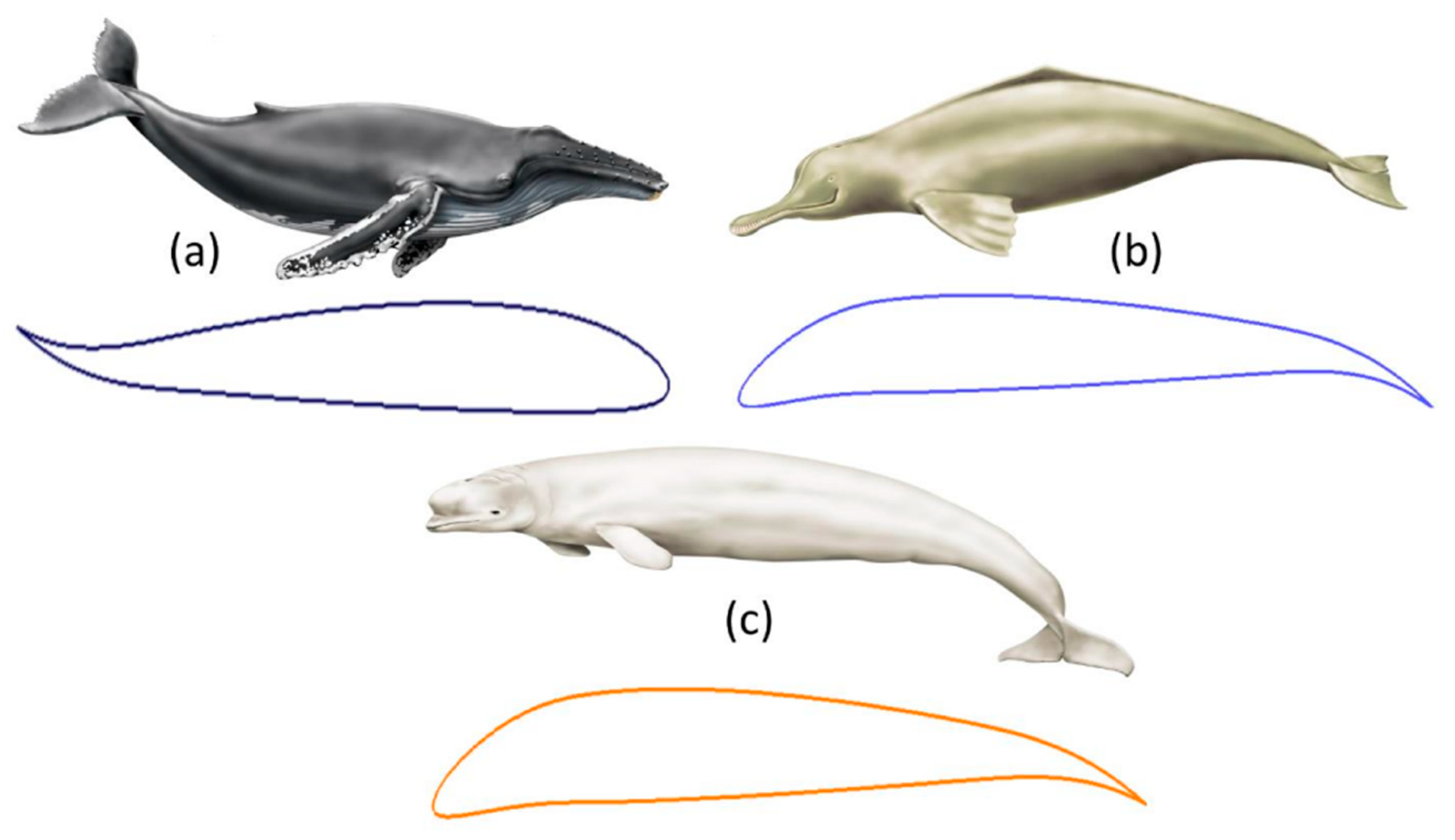
Figure 2.
Geometrical definition of a variable camber line.
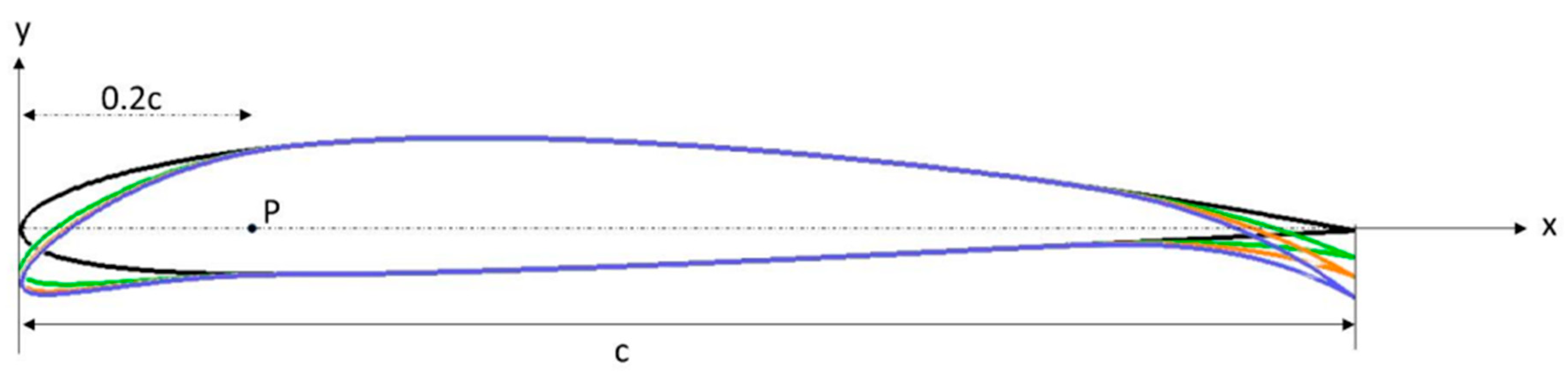
Figure 3.
Numerical modeling of a camber line [48].
Figure 3.
Numerical modeling of a camber line [48].
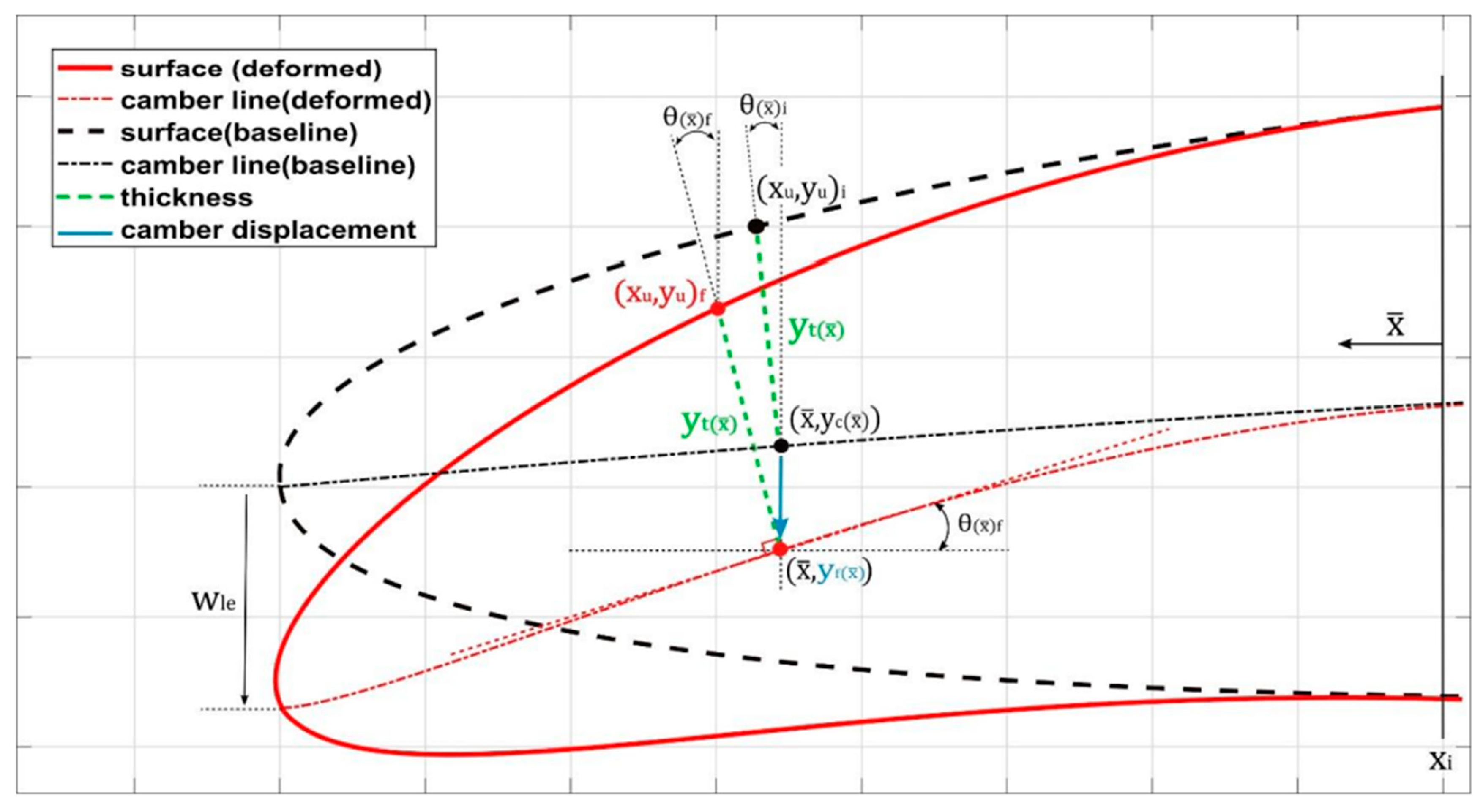
Figure 4.
Computational domain with (a) overall mesh, (b) mesh around the reference airfoil, (c) mesh around the downward morphing airfoil, (d) mesh around the upward morphing airfoil, and (d) mesh around the asynchronous morphing airfoil.
Figure 4.
Computational domain with (a) overall mesh, (b) mesh around the reference airfoil, (c) mesh around the downward morphing airfoil, (d) mesh around the upward morphing airfoil, and (d) mesh around the asynchronous morphing airfoil.
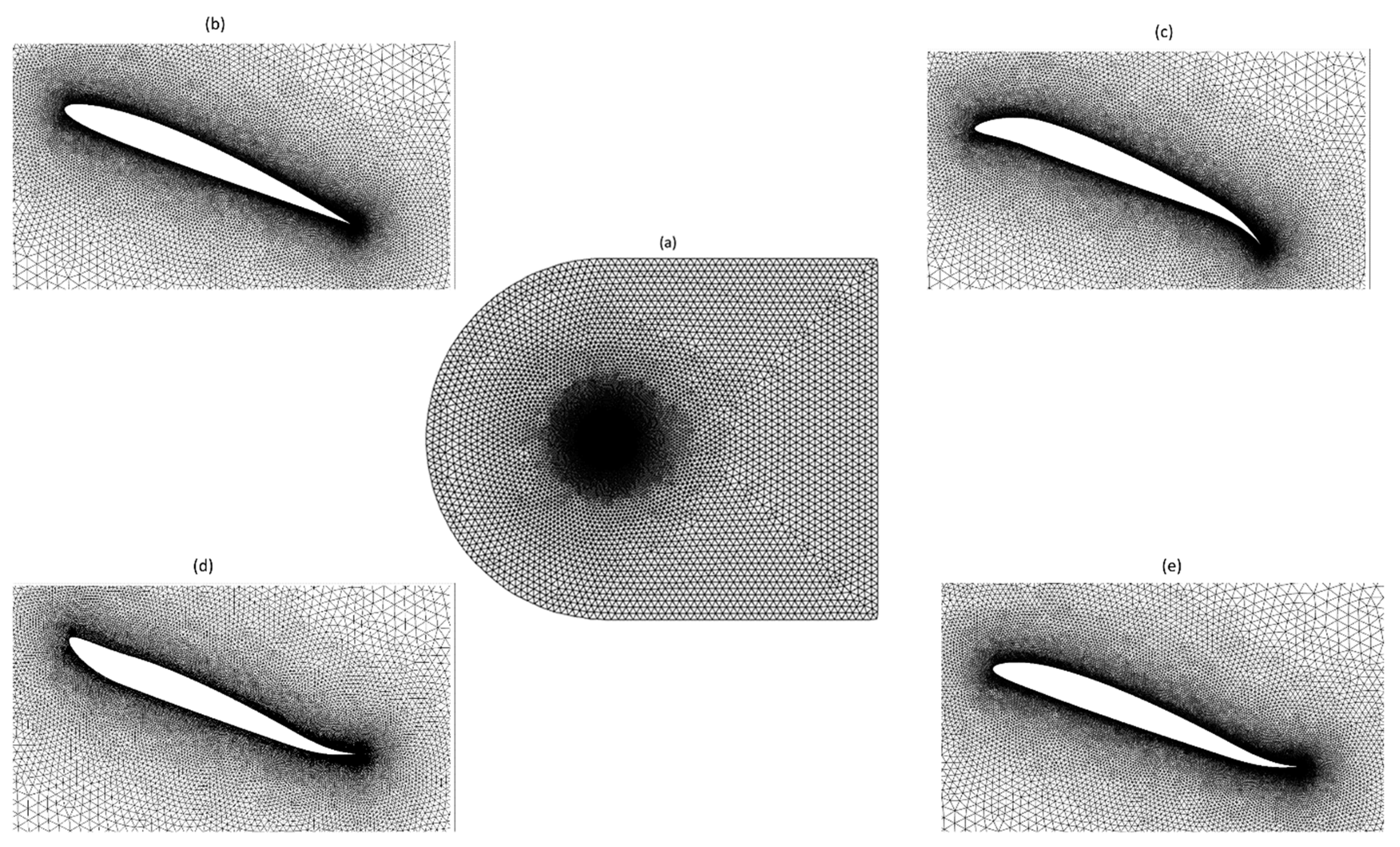
Figure 5.
Time history of the (a) lift coefficient and (b) the drag coefficient.
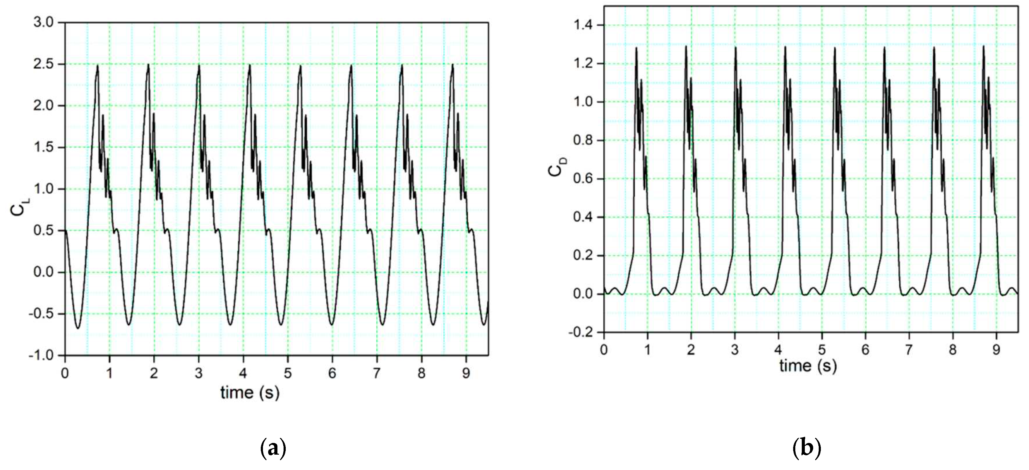
Figure 6.
Comparisons of the numerical results for the lift coefficient versus the angle of attack for three different grid sizes.
Figure 6.
Comparisons of the numerical results for the lift coefficient versus the angle of attack for three different grid sizes.
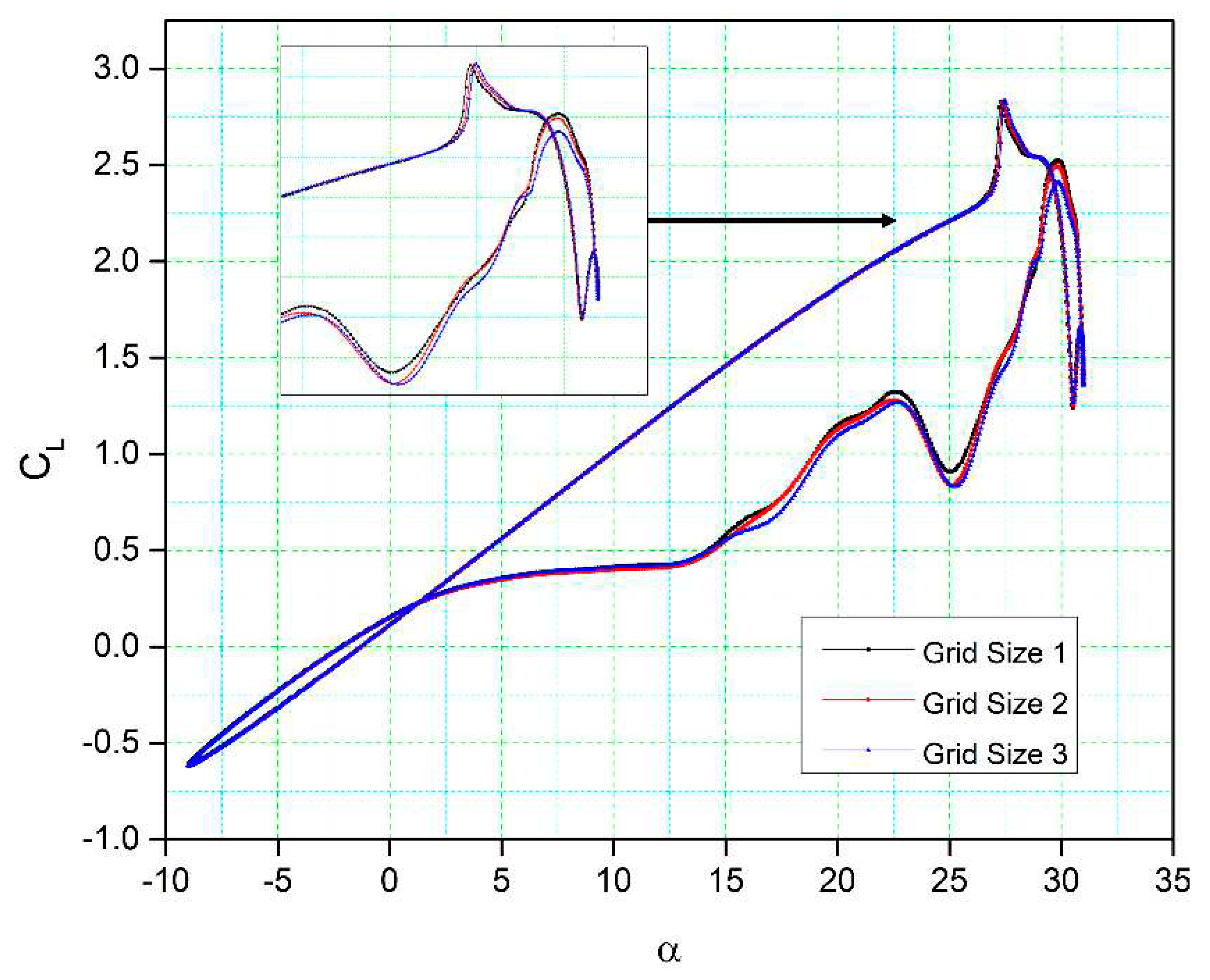
Figure 7.
Comparison of our numerical results with experimental results obtained from wind tunnel tests [51] and numerical results [50]: (a) lift coefficient; (b) drag coefficient variations with the angle of attack.
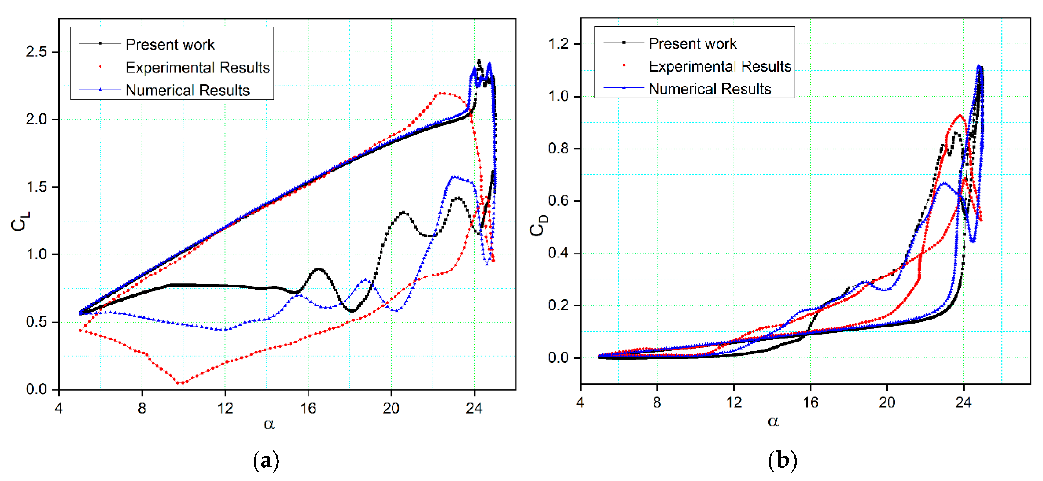
Figure 8.
CoMpLETE airfoil for three different cases at 0.5 Hz, 1 Hz, and 2 Hz with (a) lift and (b) drag coefficient transient responses at an angle of attack of 22°.
Figure 8.
CoMpLETE airfoil for three different cases at 0.5 Hz, 1 Hz, and 2 Hz with (a) lift and (b) drag coefficient transient responses at an angle of attack of 22°.
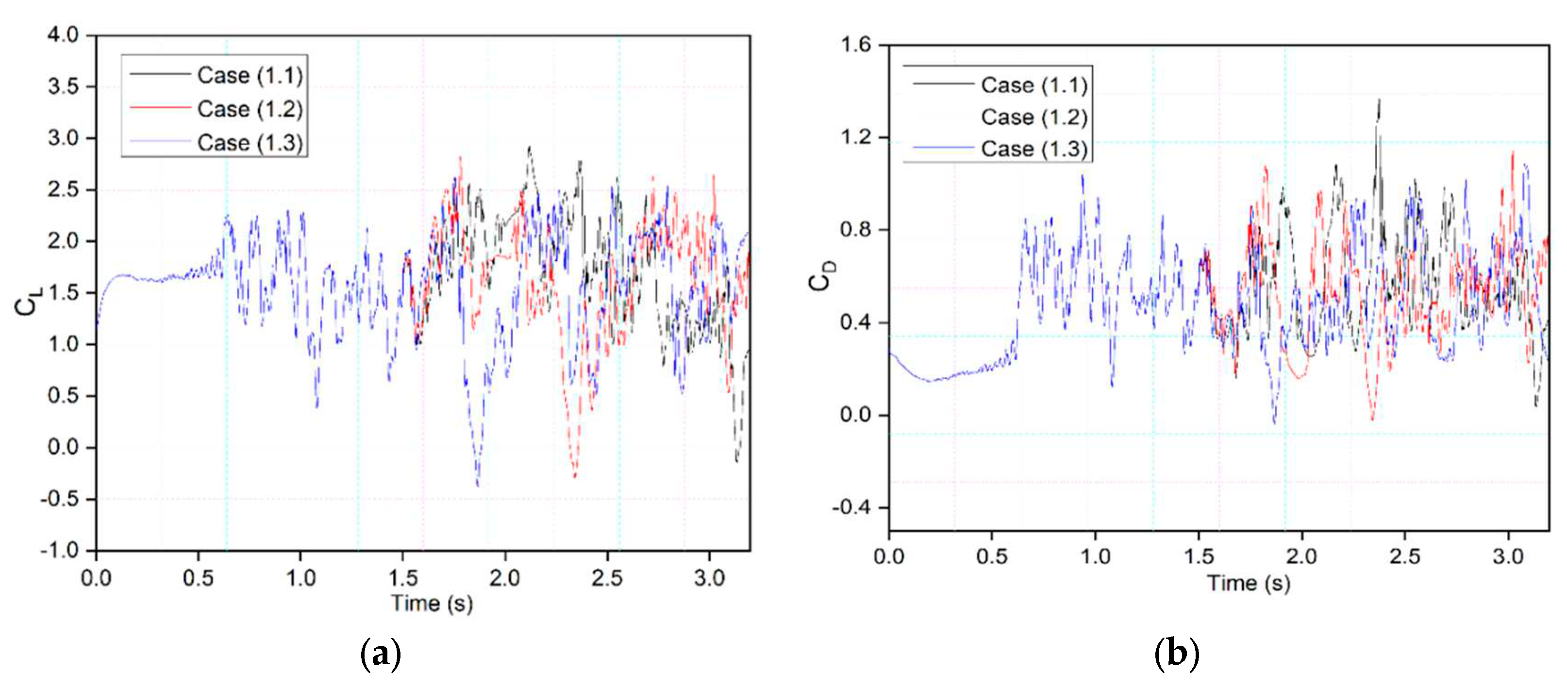
Figure 9.
Power spectral density of lift coefficient for CoMpLETE airfoil for three different cases at 0.5 Hz, 1 Hz and 2 Hz.
Figure 9.
Power spectral density of lift coefficient for CoMpLETE airfoil for three different cases at 0.5 Hz, 1 Hz and 2 Hz.
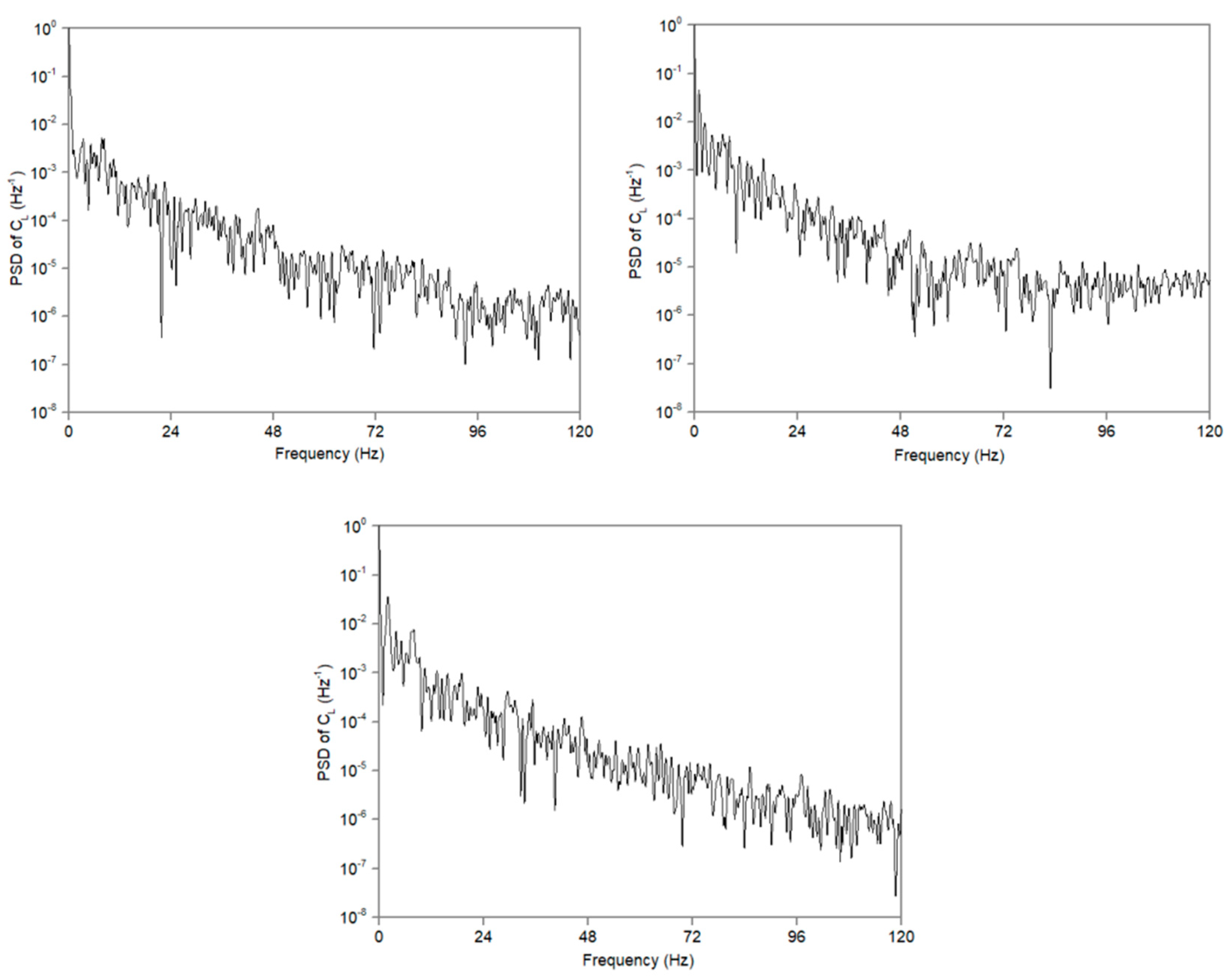
Figure 10.
Instantaneous speed responses for CoMpLETE airfoil at (a) 0.5 Hz, (b) 1 Hz, and (c) 2 Hz, at an angle of attack of 22°.
Figure 10.
Instantaneous speed responses for CoMpLETE airfoil at (a) 0.5 Hz, (b) 1 Hz, and (c) 2 Hz, at an angle of attack of 22°.
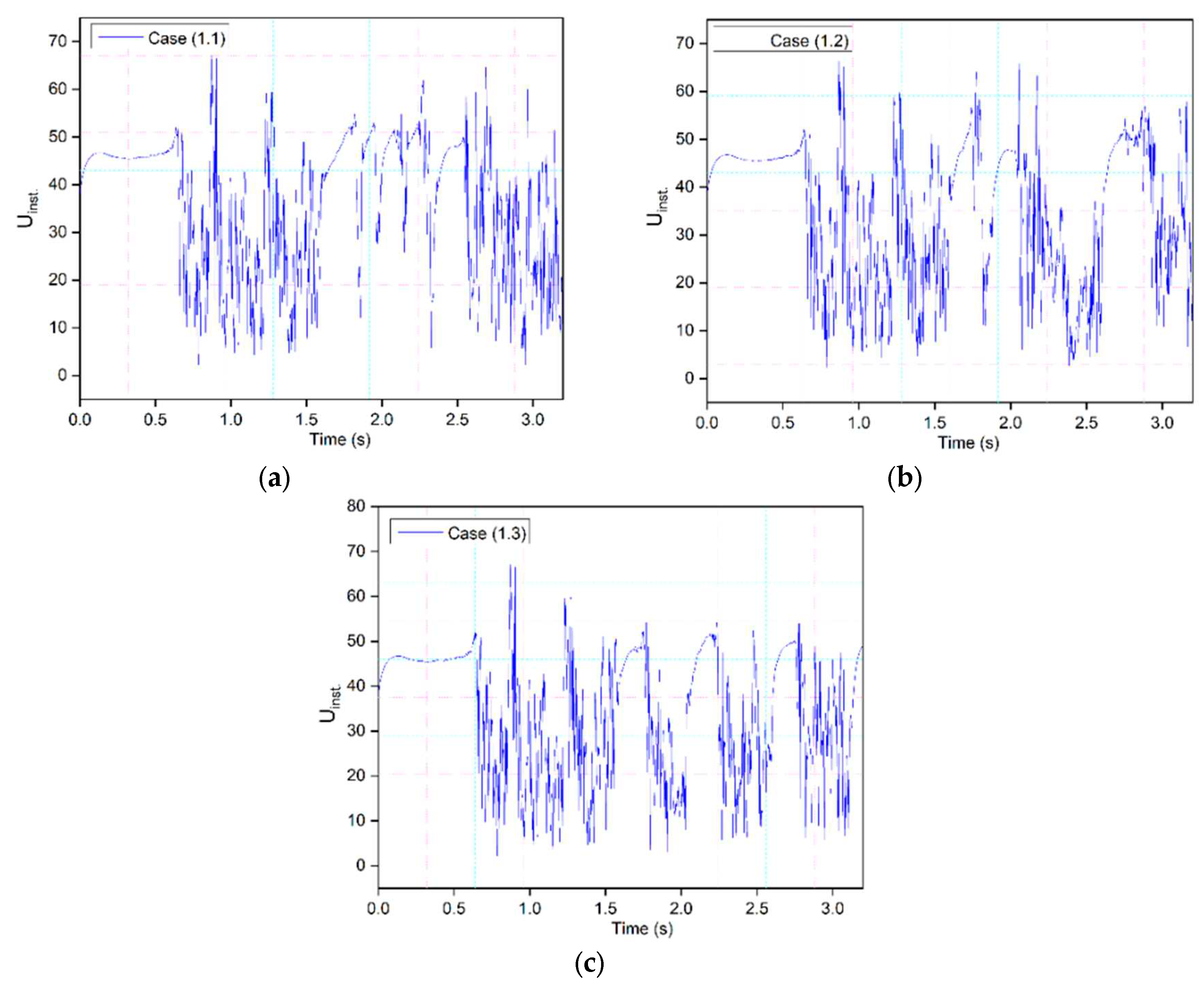
Figure 11.
Pressure coefficients accompanied by velocity streamline and vorticity contours at different time steps for (a) Case ‘1.1’ and (b) Case ‘1.2.’.
Figure 11.
Pressure coefficients accompanied by velocity streamline and vorticity contours at different time steps for (a) Case ‘1.1’ and (b) Case ‘1.2.’.
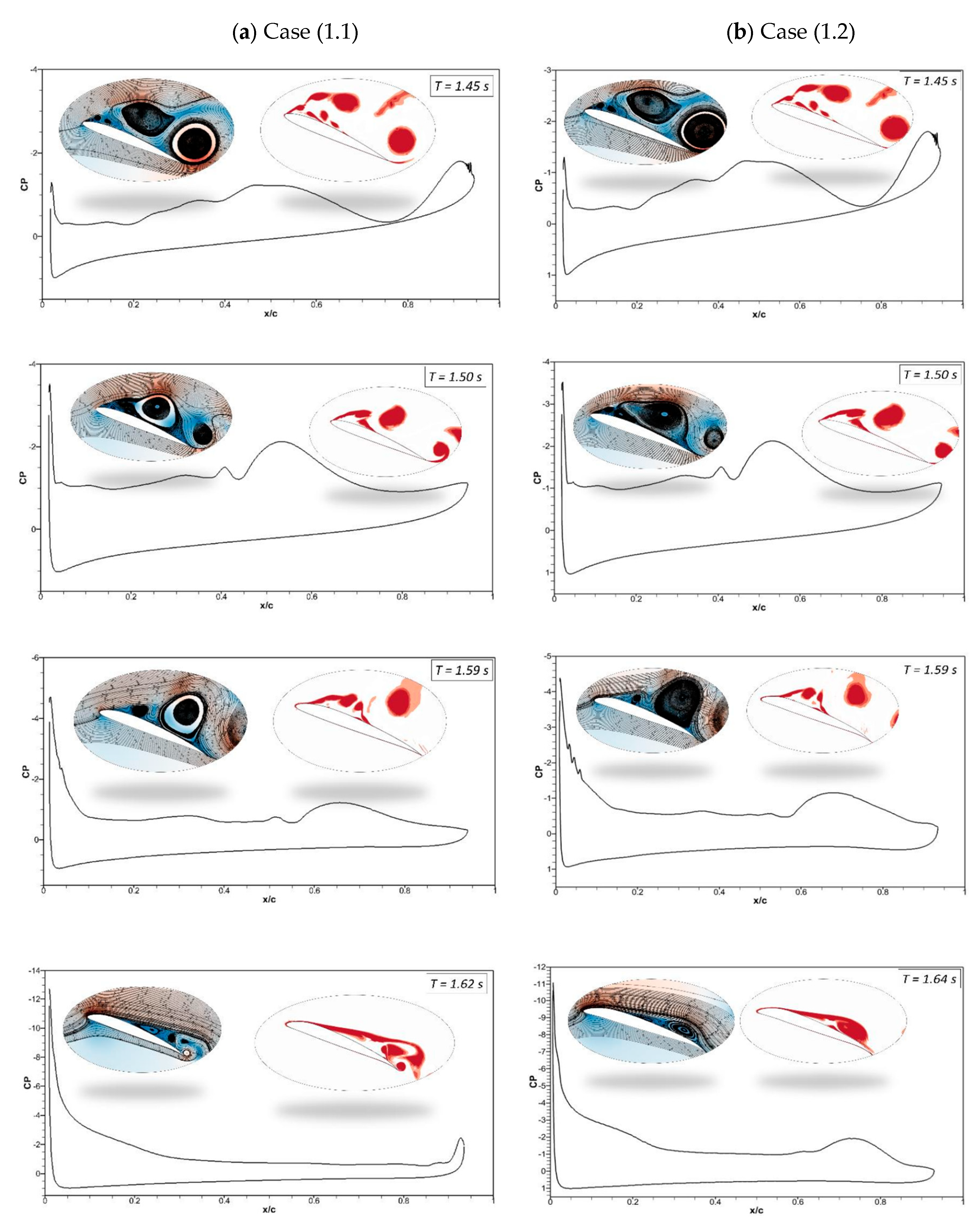
Figure 12.
Pressure coefficients, velocity streamline and vorticity contours at different time steps for (a) Case ‘1.1’ and (b) Case ‘1.2.’.
Figure 12.
Pressure coefficients, velocity streamline and vorticity contours at different time steps for (a) Case ‘1.1’ and (b) Case ‘1.2.’.
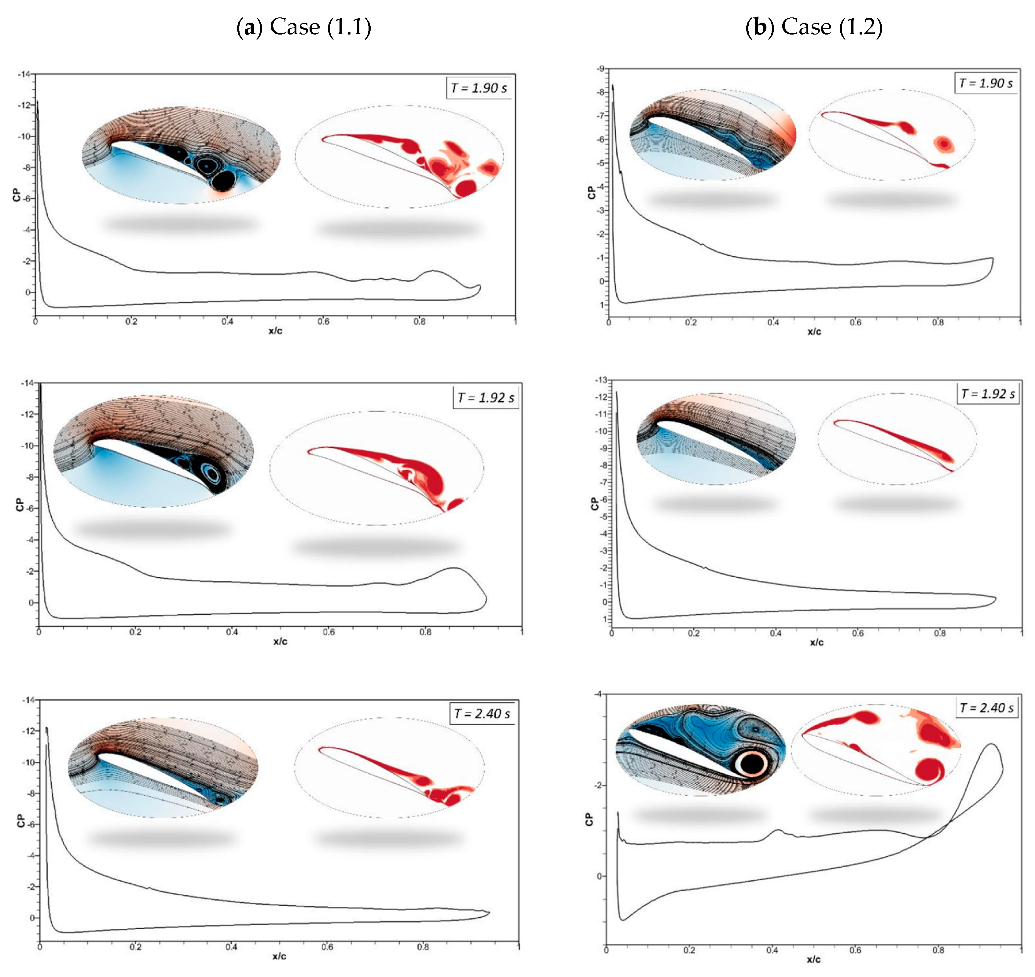
Figure 13.
CoMpLETE airfoil for Cases 1.4 with (a) lift and (b) drag coefficient transient responses, at an angle of attack of 22°.
Figure 13.
CoMpLETE airfoil for Cases 1.4 with (a) lift and (b) drag coefficient transient responses, at an angle of attack of 22°.
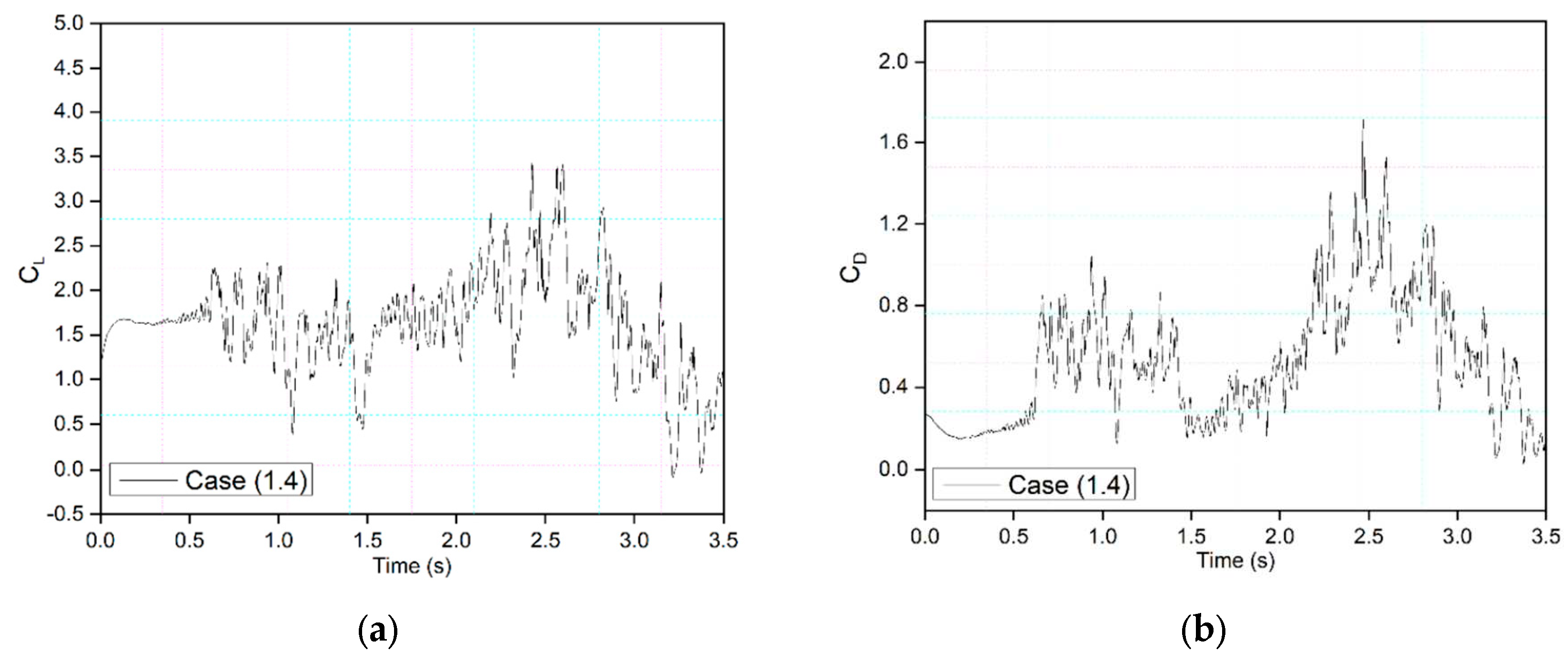
Figure 14.
CoMpLETE airfoil for Cases 1.5 with (a) lift and (b) drag coefficient transient responses at an angle of attack of 22°.
Figure 14.
CoMpLETE airfoil for Cases 1.5 with (a) lift and (b) drag coefficient transient responses at an angle of attack of 22°.
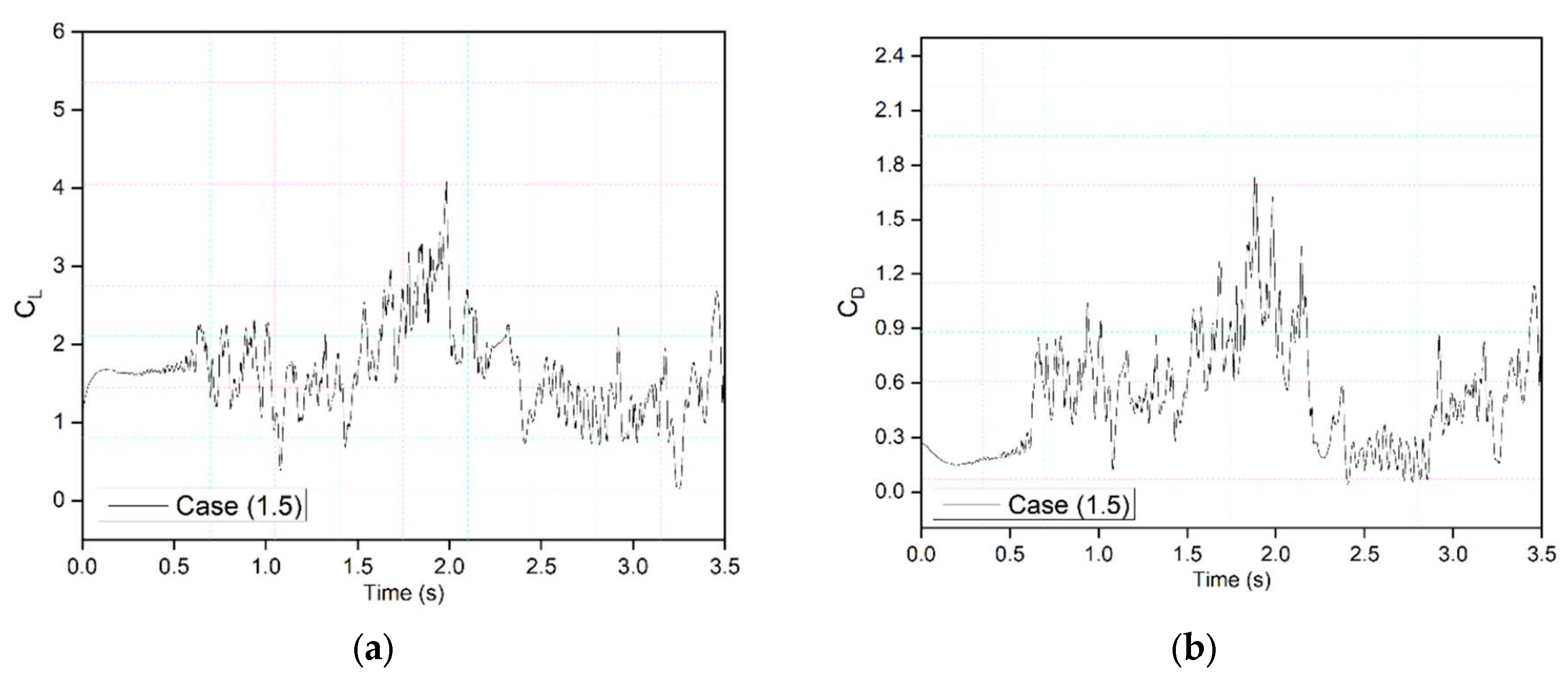
Figure 15.
Comparison of transient lift coefficient for Case (1.4) and (1.5) at 0.5 Hz, (b) Comparison of instantaneous velocity response for Case (1.4) and (1.5) at 0.5 Hz.
Figure 15.
Comparison of transient lift coefficient for Case (1.4) and (1.5) at 0.5 Hz, (b) Comparison of instantaneous velocity response for Case (1.4) and (1.5) at 0.5 Hz.
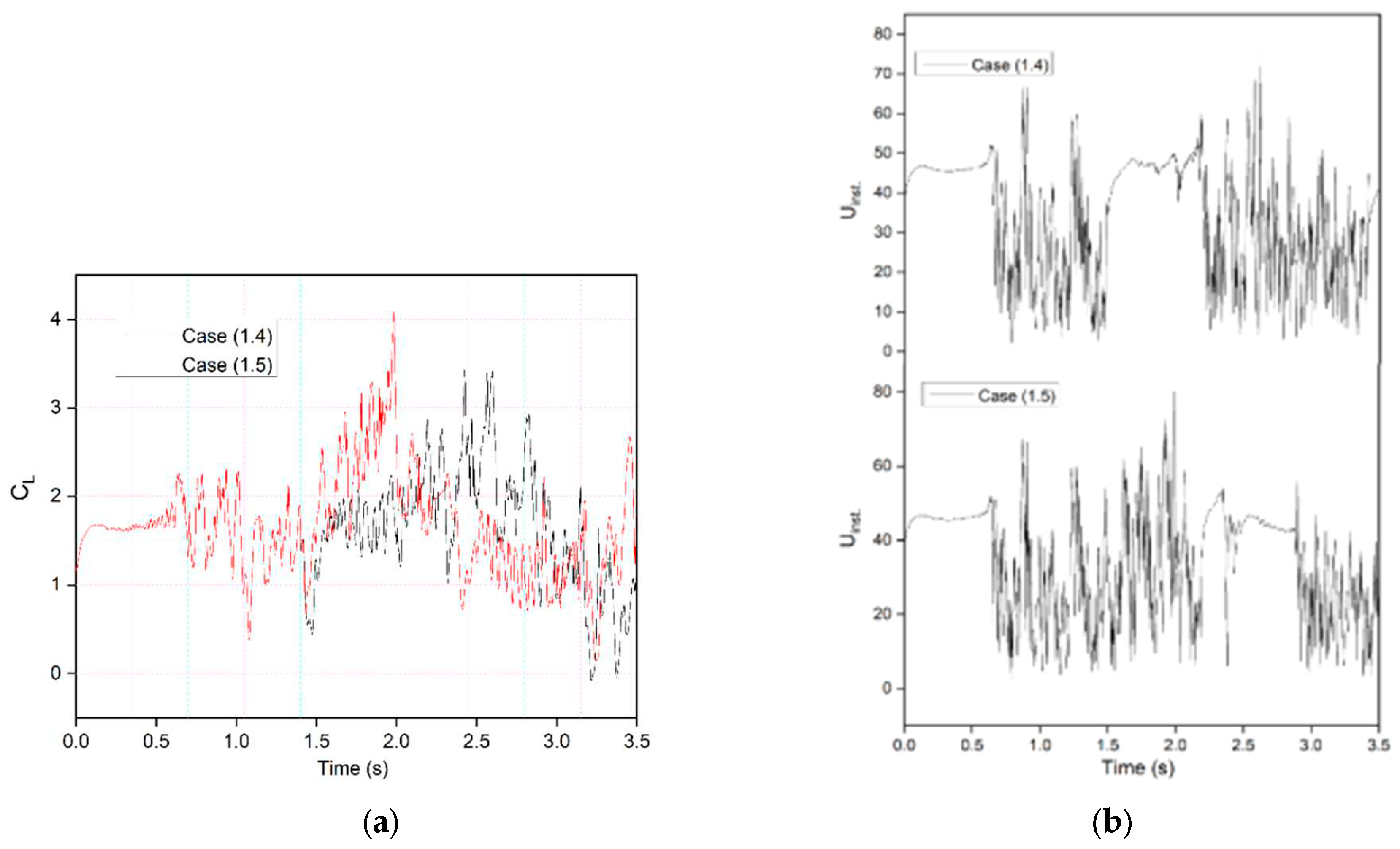
Figure 16.
CoMpLETE airfoil for three different Cases with (a) lift and (b) drag coefficient transient responses at an angle of attack of 22°.
Figure 16.
CoMpLETE airfoil for three different Cases with (a) lift and (b) drag coefficient transient responses at an angle of attack of 22°.
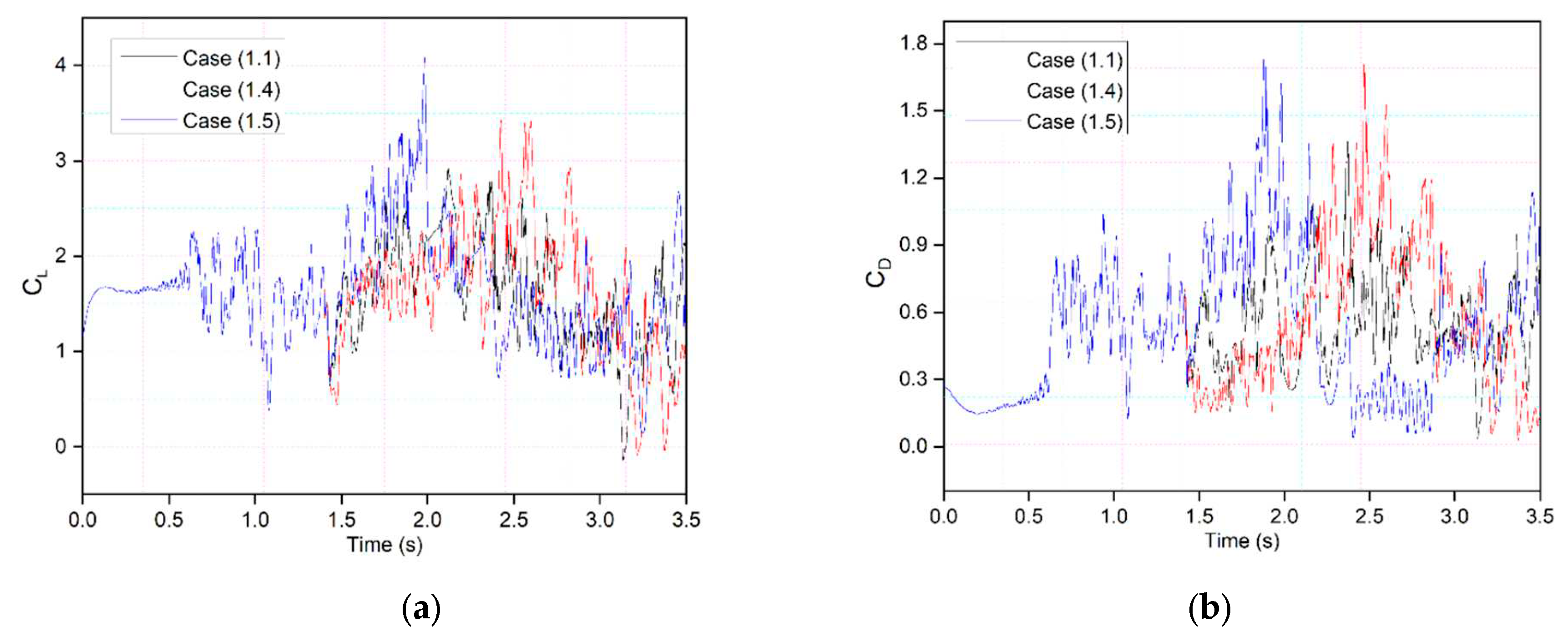
Figure 17.
Comparison of transient lift coefficient for Case (1.4) and (1.5) at 0.5 Hz, (b) Comparison of instantaneous velocity response for Case (1.4) and (1.5) at 0.5 Hz.
Figure 17.
Comparison of transient lift coefficient for Case (1.4) and (1.5) at 0.5 Hz, (b) Comparison of instantaneous velocity response for Case (1.4) and (1.5) at 0.5 Hz.
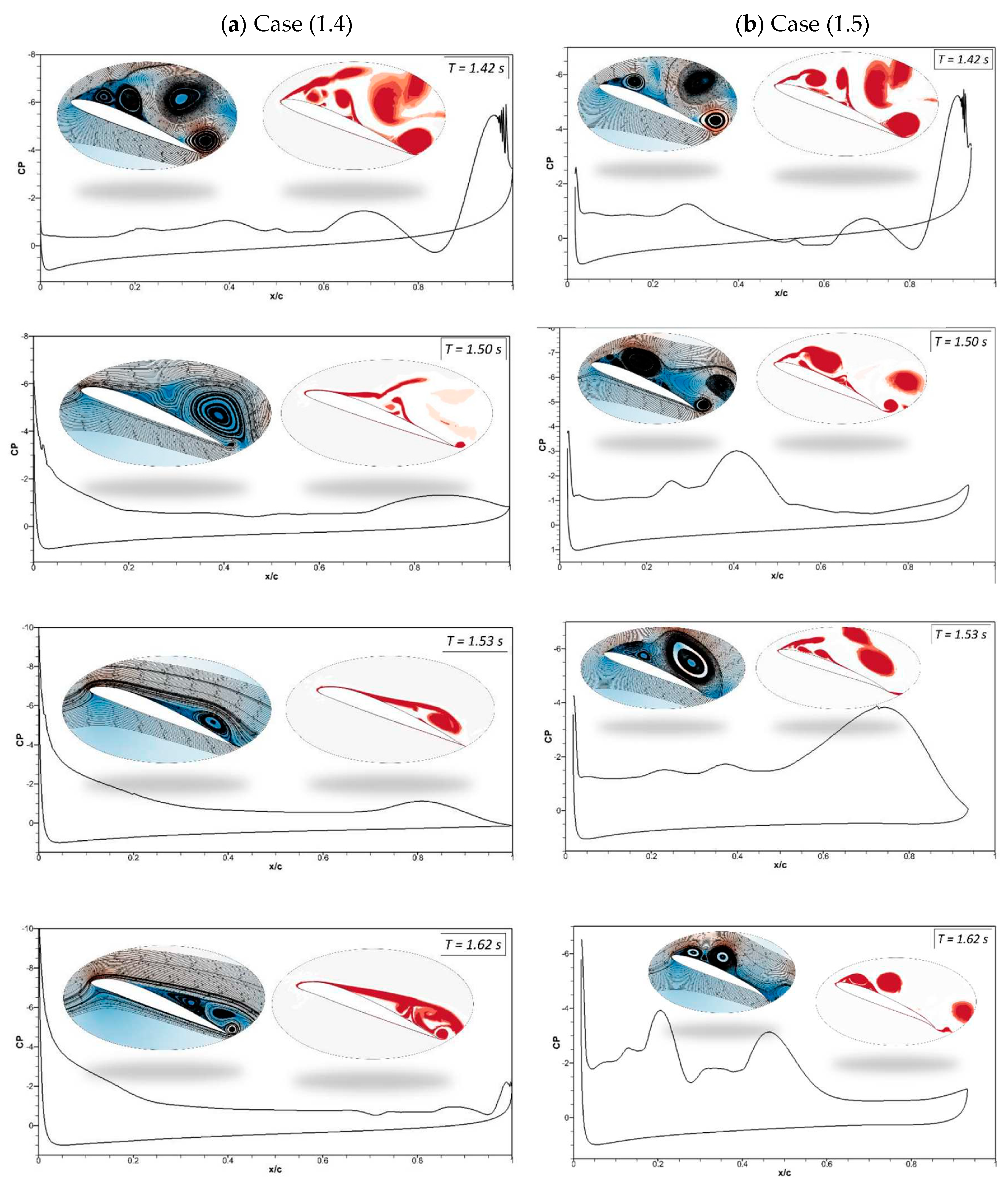
Figure 18.
Comparison of transient lift coefficient for Case (1.4) and (1.5) at 0.5 Hz, (b) Comparison of instantaneous velocity response for Case (1.4) and (1.5) at 0.5 Hz.
Figure 18.
Comparison of transient lift coefficient for Case (1.4) and (1.5) at 0.5 Hz, (b) Comparison of instantaneous velocity response for Case (1.4) and (1.5) at 0.5 Hz.
Figure 19.
CoMpLETE airfoil for Case 2.1 with (a) lift and (b) drag coefficient transient responses at an angle of attack of 22°.
Figure 19.
CoMpLETE airfoil for Case 2.1 with (a) lift and (b) drag coefficient transient responses at an angle of attack of 22°.
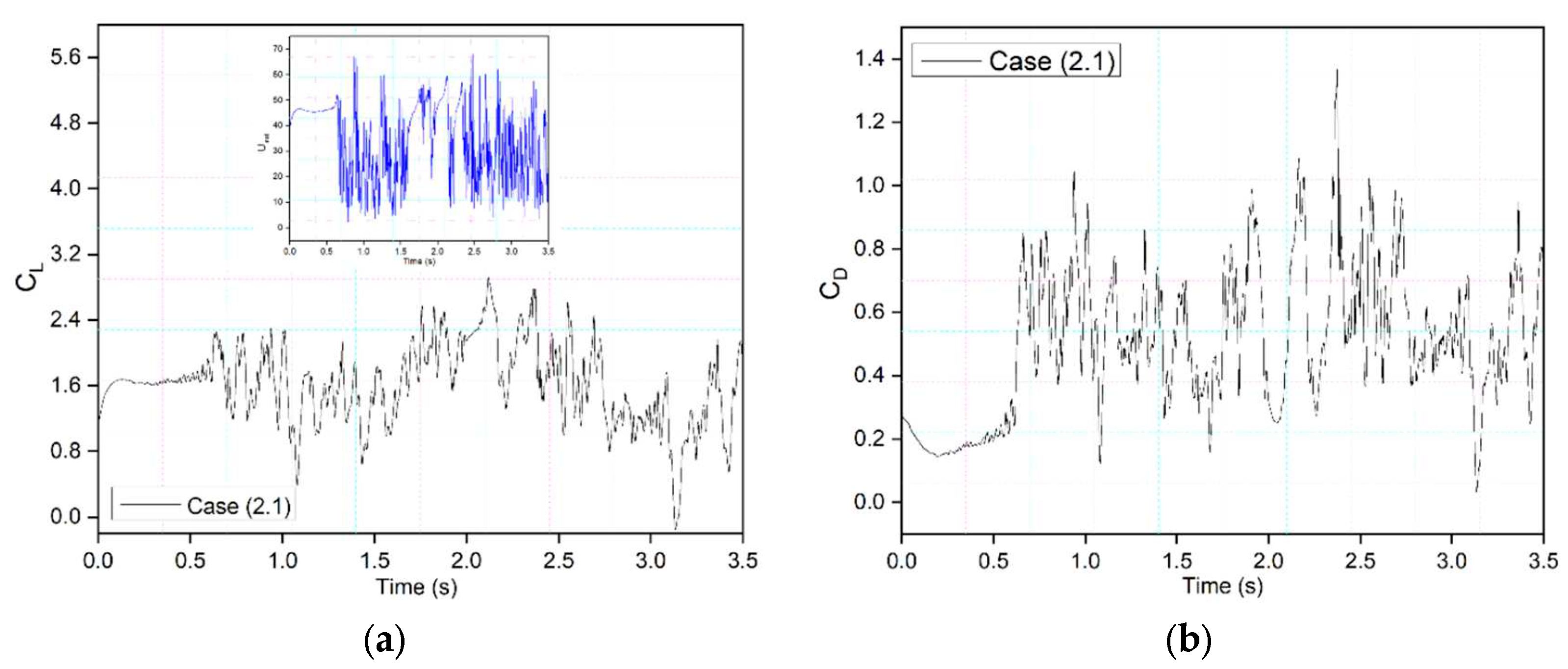
Figure 20.
Comparison of transient (a) lift and (b) drag coefficient for Case 1.2 and Case 2.2 at 1 Hz.
Figure 20.
Comparison of transient (a) lift and (b) drag coefficient for Case 1.2 and Case 2.2 at 1 Hz.
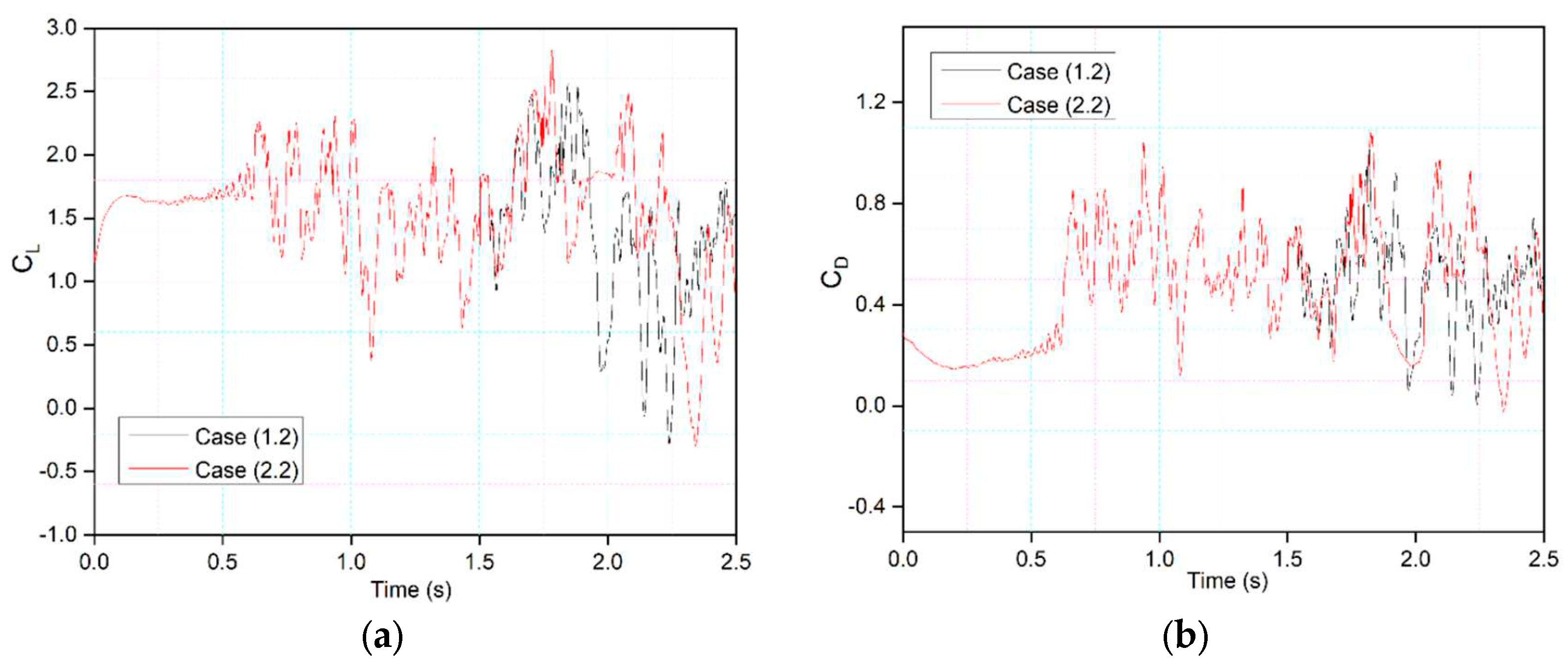
Figure 21.
Pressure coefficients, velocity streamline and vorticity contours at different time steps for (a) Case ‘1.2’ and (b) Case ‘2.2’.
Figure 21.
Pressure coefficients, velocity streamline and vorticity contours at different time steps for (a) Case ‘1.2’ and (b) Case ‘2.2’.
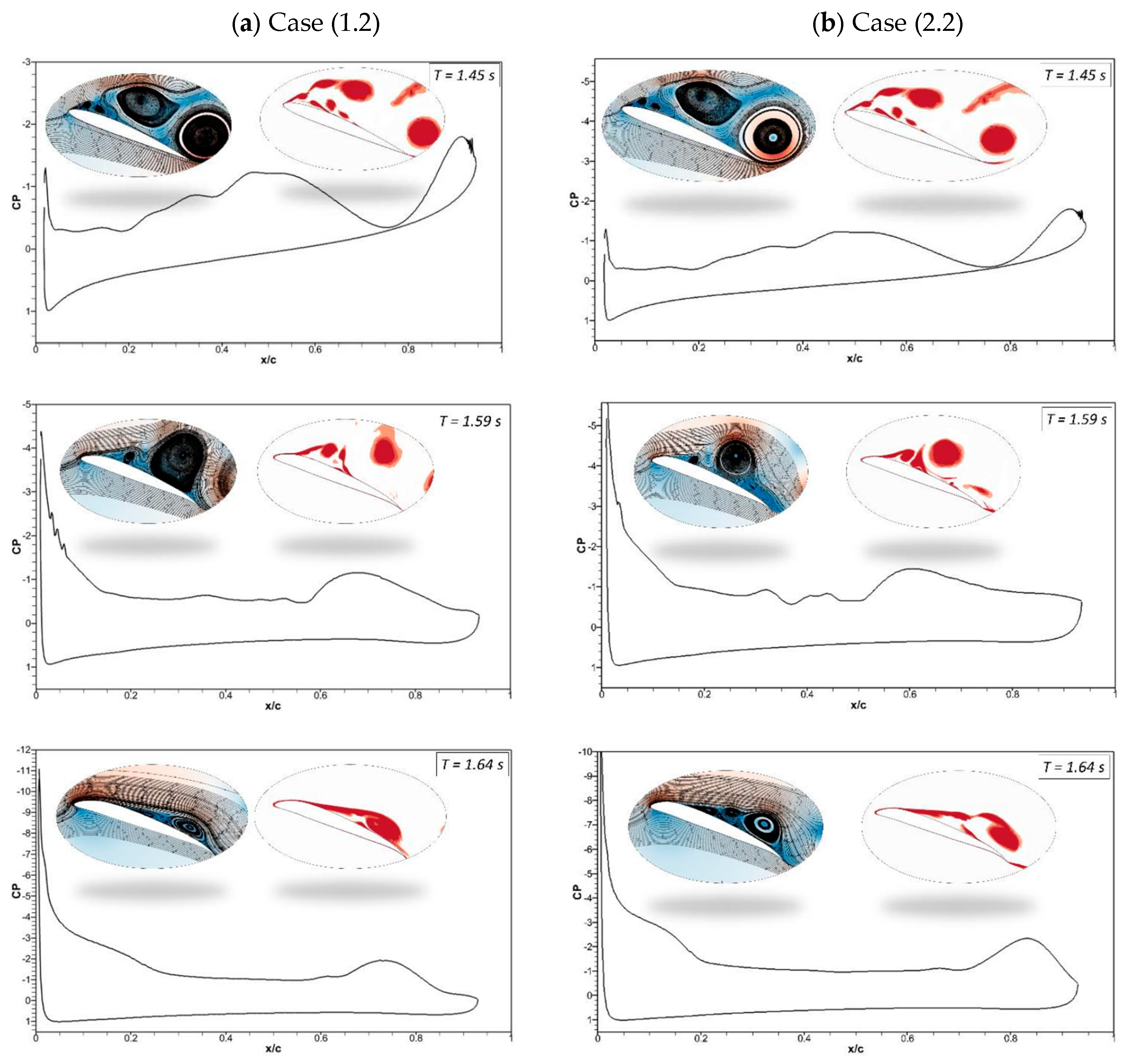
Figure 22.
Comparison of transient (a) lift and (b) drag coefficient for Case 1.2 and Case 2.2 at 0.5 Hz.
Figure 22.
Comparison of transient (a) lift and (b) drag coefficient for Case 1.2 and Case 2.2 at 0.5 Hz.

Figure 23.
Comparison of transient (a) lift and (b) drag coefficient for Case 1.2 and Case 2.2 at 0.5 Hz.
Figure 23.
Comparison of transient (a) lift and (b) drag coefficient for Case 1.2 and Case 2.2 at 0.5 Hz.
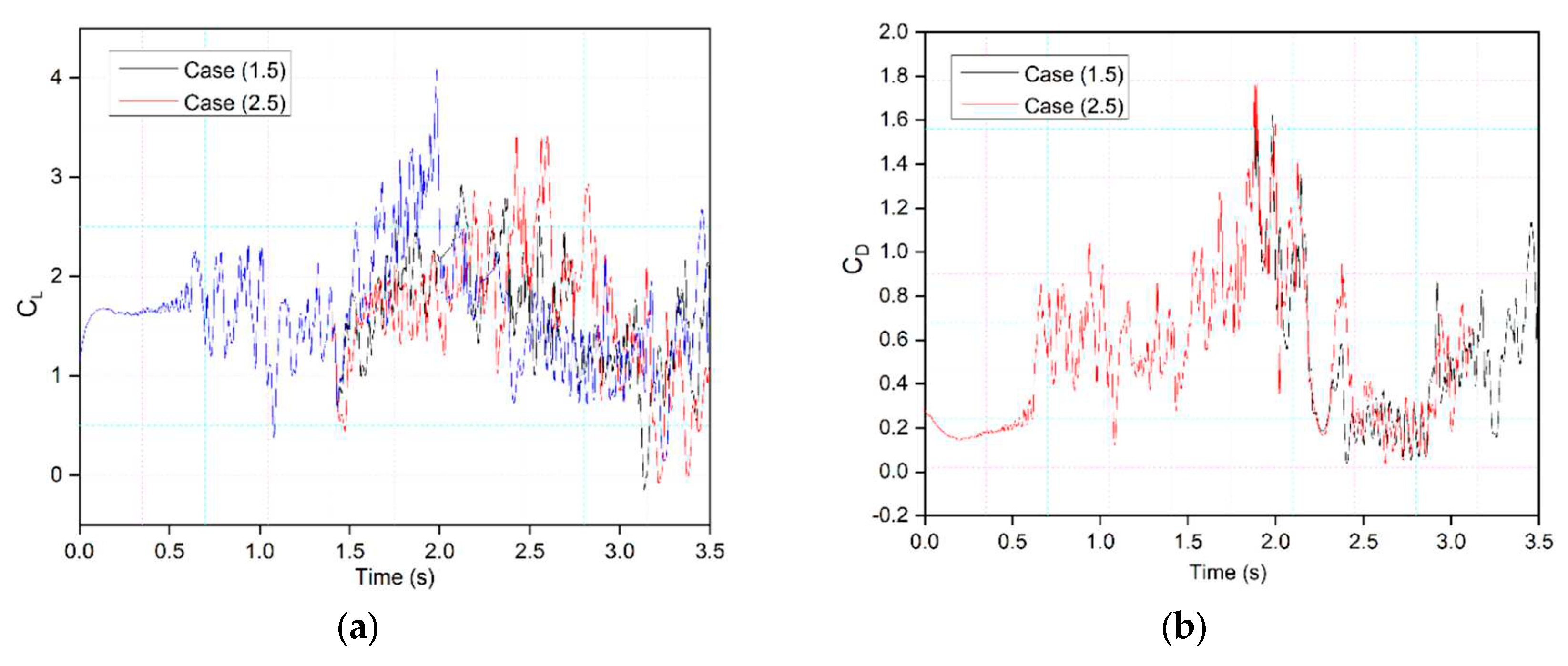
Figure 24.
Pressure coefficients, velocity streamline and vorticity contours at different time steps for (a) Case ‘1.4’ and (b) Case ‘2.4’.
Figure 24.
Pressure coefficients, velocity streamline and vorticity contours at different time steps for (a) Case ‘1.4’ and (b) Case ‘2.4’.
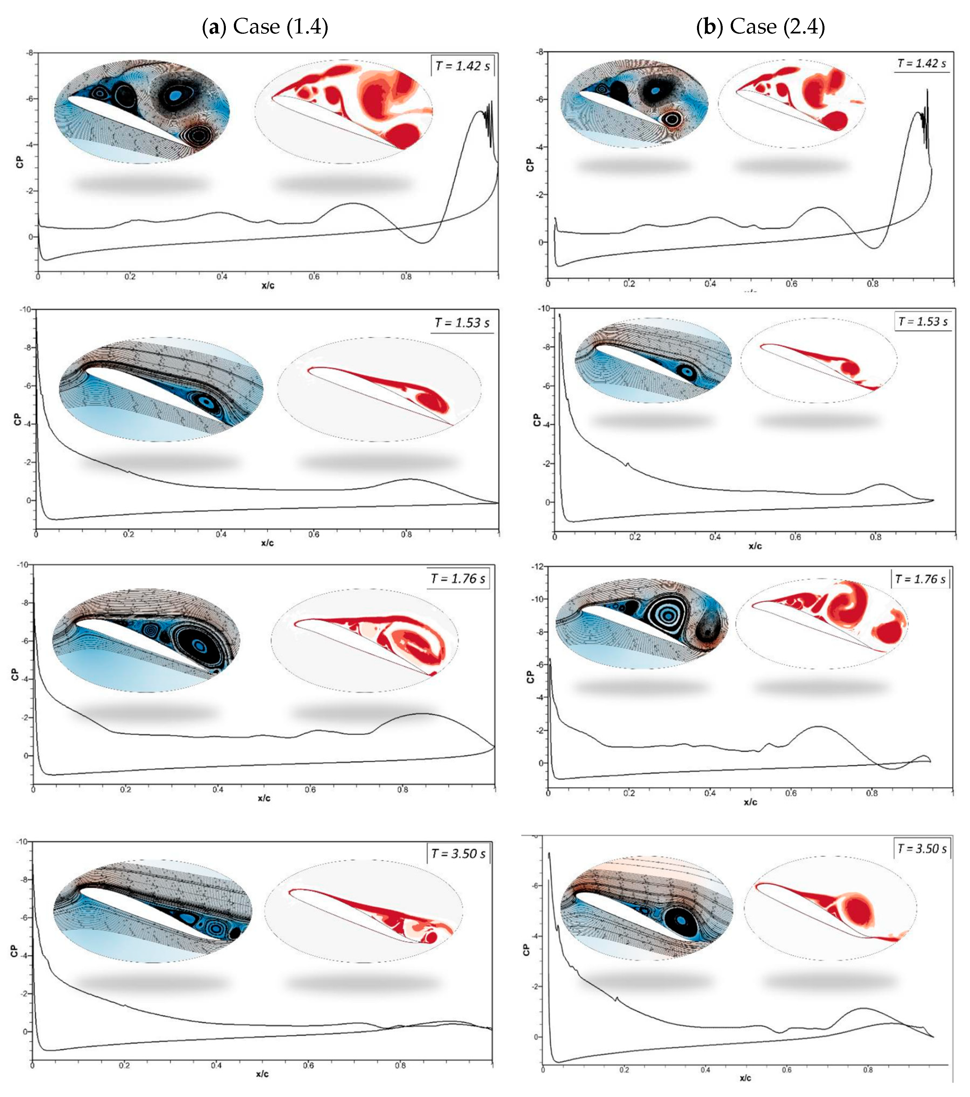

Table 1.
Airfoil with morphing of the leading edge starts at 0.2c, and the trailing edge morphing starts at 0.75c.
Table 1.
Airfoil with morphing of the leading edge starts at 0.2c, and the trailing edge morphing starts at 0.75c.
| Morphing Case | Leading Edge Morphing Starting Time (seconds) | Trailing Edge Morphing Starting Time (seconds) | Morphing Deflection Frequency (Hz) |
|---|---|---|---|
| Case 1.1 | T= 1.5 | T = 1.5 | 0.5 |
| Case 1.2 | T= 1.5 | T = 1.5 | 1 |
| Case 1.3 | T= 1.5 | T = 1.5 | 2 |
| Case 1.4 | T = 1.4 | T = 1.85 | 0.5 |
| Case 1.5 | T = 1.85 | T = 1.4 | 0.5 |
| Case 1.6 | T = 1.4 | T = 1.85 | 1 |
| Case 1.7 | T = 1.85 | T = 1.4 | 1 |
Table 2.
Airfoil with morphing of the leading edge starts at 0.15c, and the trailing edge morphing starts at 0.75c.
Table 2.
Airfoil with morphing of the leading edge starts at 0.15c, and the trailing edge morphing starts at 0.75c.
| Morphing Case | Leading Edge Morphing Starting Time (seconds) | Trailing Edge Morphing Starting Time (seconds) | Morphing Deflection Frequency (Hz) |
|---|---|---|---|
| Case 2.1 | T= 1.5 | T = 1.5 | 0.5 |
| Case 2.2 | T= 1.5 | T = 1.5 | 1 |
| Case 2.3 | T= 1.5 | T = 1.5 | 2 |
| Case 2.4 | T = 1.4 | T = 1.85 | 0.5 |
| Case 2.5 | T = 1.85 | T = 1.4 | 0.5 |
Table 3.
Grid properties of the three grid sizes for the grid-sensitivity analysis.
| Grid Size | Number of cells | Min length | Max length | Bias factor |
|---|---|---|---|---|
| 1 | 62 626 | 0.001 | 0.06 | 1.12 |
| 2 | 103 212 | 0.001 | 0.035 | 1.08 |
| 3 | 206 038 | 0.001 | 0.02 | 1.05 |
Disclaimer/Publisher’s Note: The statements, opinions and data contained in all publications are solely those of the individual author(s) and contributor(s) and not of MDPI and/or the editor(s). MDPI and/or the editor(s) disclaim responsibility for any injury to people or property resulting from any ideas, methods, instructions or products referred to in the content. |
© 2023 by the authors. Licensee MDPI, Basel, Switzerland. This article is an open access article distributed under the terms and conditions of the Creative Commons Attribution (CC BY) license (http://creativecommons.org/licenses/by/4.0/).
Copyright: This open access article is published under a Creative Commons CC BY 4.0 license, which permit the free download, distribution, and reuse, provided that the author and preprint are cited in any reuse.


