
Submitted:
20 December 2023
Posted:
21 December 2023
You are already at the latest version
Abstract
Abstract: This study estimates consumers’ willingness to pay (WTP) for sustainability turfgrass attributes such as low-input and stress-tolerance attributes, while considering potential trade-off relationships between aesthetic attributes and sustainability attributes. To address our objectives, our study conducts a choice experiment and estimates two mixed logit models. The first model includes low-input, winter kill, and shade-tolerance attributes as predictor variables, and the second model extends the first model by adding interaction terms between aesthetic and sustainability attributes. Another choice experiment is conducted under water policies with various water rate increase and watering restriction scenarios. Results from the mixed logit models show that overall, higher low-input cost reduction, less winter-damaged, and more shade-tolerance grasses are preferred, the direct effect of aesthetic attributes on consumers’ preference is strong, but the indirect effect represented by the interaction terms are generally statistically insignificant. Our results indicate that consumers like to have a pretty lawn, but no strong consideration is given to the aesthetics of their lawn when selecting low-input and stress-tolerance turfgrasses. Our choice experiment under water policy scenarios suggests that water pricing is more effective than watering restriction in increasing consumer demand for water-conserving turfgrasses.
Keywords:
turfgrass attribute
; missing attribute
; trade-off relationship
; water conservation policy
1. Introduction
Non-market valuation is an important research topic of various economics and marketing research, and choice experiment (CE) is a commonly used method to conduct such research. In CE, participants are asked to choose one alternative from a set of choice tasks consisting of different bundles of attribute levels. Then, the CE data are used to estimate respondents’ preferences for each attribute (or each level of an attribute). One concern about CE choice experiment is that including or excluding certain characteristics of a product may lead to a biased estimator in econometrics [1,2,3]. Despite this concern, only limited CE studies in agricultural and environmental economics have paid attention to this issue, and CEs for turfgrass research rarely address this issue. In general, many turfgrass studies using CE have focused on estimating consumer preferences for low-input attributes such as water, mowing, and fertilizer requirement without considering a potential relationship between aesthetic attributes and attributes of low-input [4,5,6,7,8,9]. It has been well known that enhancing low-input attributes tends to have negative influence on the aesthetics of lawn. For example, Ghimire et al. (2016) [5] and Ghimire et al. (2019) [6] estimate WTPs for turfgrass attributes of maintenance cost reduction but do not include turfgrass aesthetic attributes in CE. A few exceptions include Hugie et al. (2012) [7], Yue et al. (2012) [8], and Yue et al. (2017) [9], which evaluate the value of low input-attributes of cool-season grasses along with aesthetic attributes (color and texture). However, no potential trade-off relationships between aesthetic and low-input attributes have been investigated in valuation of consumer preference for the low-input attributes in these studies.
This study estimates consumers’ WTP for low input and stress-tolerance attributes of warm-season turfgrasses, while considering potential negative effect of enhancing these attributes on the aesthetics of grasses. Our study extends earlier studies in three ways. First, we consider the potential negative impact of enhancing low-input and stress-tolerance attributes on aesthetic characteristics of turfgrasses in CE. Using the CE data, mixed logit models are estimated with sustainability (low-input, stress-tolerance) and aesthetic attributes as explanatory variables with and without interaction terms between each of sustainability attributes and color, density, and texture of grasses. Then, we test coefficients of the interaction terms for the potential trade-off relationships between variables that are interacted each other. This attempt should be important in evaluating consumer preferences for the improved turfgrass attributes accurately. In particular, from the perspective of breeders who develop new turfgrasses with enhanced traits, it would be most helpful to know how households evaluate the potential trade-off relationship between aesthetic and sustainability attributes for the development of new turfgrass varieties in the future. Second, our study evaluates consumers’ preference for the sustainability attributes of warm-season grasses by surveying households residing in the southern region. As we focus on enhancing warm-season grasses, our study incorporates winter kill attribute with consideration of all three aesthetic attributes: color, density, and texture. Warm-season grasses, e.g., bermudagrass, tend to be sensitive to winter damage. As a result, density should be one of important features of the aesthetics of warm-season grasses along with color and texture. Finally, our study investigates whether water conservation policies impact consumers' valuation of low-input attributes, particularly water conservation attributes. To date, many studies evaluating effects of water conservation policies have focused on policy effects on water preservation [10,11,12]. Unlike these studies, our study evaluates the impact of these polices on consumer preferences for water conservation turfgrass attribute.
2. Literature Review
Developing low-input and stress-tolerance varieties has been major research interests for many turfgrass breeders. Low-input grasses have been demanded by homeowners because of prolonged drought in many parts of the world and potential negative environmental externalities caused by overuse of chemical inputs such as fertilizer, pesticides, and herbicides and weather variability [8]. Stress-tolerance turfgrasses have also been developed because more arable lands become salinized, and harsher winter conditions such as bitter cold and icy weather conditions cause more damage or death of grasses. Therefore, recent studies evaluating economic values of developing new and enhanced turfgrass varieties have mostly focused on the valuation of low-input and stress-tolerance attributes [5,6,7,8,9]. Ghimire et al. (2016) [5] attempt to elicit homeowners’ preference on low-input attributes such as water requirement and maintenance cost for lawn care and stress tolerance attributes such as lost lawn area to winter kill, shade tolerance, and salinity tolerance. Empirical results indicate that participants most prefer low maintenance cost, and the second, third, and fourth preferred attributes are less water requirement, shade tolerance, and saline tolerance, respectively. Ghimire et al. (2019) [6] extend the previous study by considering group heterogeneity. Two groups such as “Willing hobby gardeners” and “Reluctant mature homeowners” are identified, and results show that, in both classes, WTPs for low and medium water requirements are the first and second highest. The two earlier studies find that the warm-season turfgrass varieties with low-input attributes are attractive choices to southern households. Yet, the appearance of turfgrass could also be an important factor when households choose turfgrass varieties [8]. Hugie et al. (2012) [7], Yue et al. (2012) [8], and Yue et al. (2017) [9] include aesthetic attributes, along with low-input attributes, in their CEs. Hugie et al. (2012) [7] find that low-input attributes are preferred to aesthetic attributes. Yue et al. (2012) [8] also consider a set of aesthetic attributes, low-input attributes, and other turfgrass characteristics for their model specifications and conclude that low-input attributes are as important as aesthetic attributes. Yue et al., (2017) [9] assess WTPs for low-input attributes and aesthetic attributes for residents of the U.S. and Canada and find that low-input attributes are more valuable traits than aesthetic traits, which is consistent with findings from Hugie et al. (2012) [7].
Although all three studies consider aesthetic attributes in CEs, the studies do not directly test for the potential interaction, trade-off, effect between low-input and aesthetic attributes. The earlier studies also focus only on color and texture of cool-season grass, while our study examines the interaction effects for warm-season grass considering color, density, and texture of grasses. In this context, Meas et al. (2015) [13] suggest that marginal effects of interacting terms between pairs of attributes be considered along with direct effects for better estimates of marginal effects of attributes. For example, a few studies in environmental economics (e.g., [14,15]) and food economics (e.g., [16,17]) use coefficients of interaction terms between attributes to identify trade-off relationships. In a typical lawn management practice, input use (e.g., the amount of water sprayed) and appearance of lawn (e.g., color of lawn) could closely interact with each other.
Various water conservation policies (e.g., increasing water rates and limiting lawn watering) have been implemented in drought areas, particularly in southern and midwestern parts of the U.S, and many earlier studies evaluate effects of these policies (e.g., [10,11,12]). Overall, the studies conclude that policies restricting outdoor water use or increasing water rates are effective in saving domestic water.1 The studies also note that demand for low-input turfgrass could increase under regulations associated with water conservation [8]. Restrictions on water use could make homeowners face challenges to maintain a healthy and good-looking lawn. As a result, it could affect consumers’ valuation of low-input attributes, particularly water-conserving attributes. Yet, currently, no studies directly estimate how water conservation regulations affect the demand for low-input turfgrass.2 In this paper, we examine how water conservation policies such as outdoor watering restrictions and water rate increases affect consumer preferences on low-input turfgrass attributes when the trade-off relationship between low-input and aesthetic attributes is considered.
3. Materials and Methods
3.1. Model
A random utility model that describes how individual i‘s utility is formed by selecting alternative j in a choice set t can be written as:
where the utility function, , consists of a deterministic component, , and a stochastic part, can be defined as observed product attributes and is corresponding coefficients. is an independently and identically distributed (i.i.d.) random error term. Allowing individuals’ preference heterogeneity, we can specify a mixed logit model (MXL) as:
where an individual-specific parameter, follows a multivariate distribution, (b, ), with mean b and variance-covariance matrix is assumed to have the extreme value distribution.
To derive an empirical model of (2), we use effect coding rather than dummy coding for all categorical variable levels to recover marginal preferences and WTPs of base levels [18]. Using the recovered baseline preference estimates, it is possible for us to calculate the relative importance of attributes, i.e., WTP rankings over attributes are calculated after estimating WTPs by attribute level. Estimates of WTP rankings by attribute, rather than attribute level, are expected to provide useful information about research priority of attributes for breeders and policy makers.
An empirical model considering low-inputs, stress-tolerance attributes, and aesthetic attributes (a model without interaction terms) is specified as:3
where ASC is the alternative specific constant to measure the utility of status quo: ASC =1 if no purchase of new turfgrass is selected, i.e., the status quo, ASC =-1 otherwise; WR1 and WR2 represent the percentage reduction of water cost: WR1= 1 if the level of the water cost reduction is 40% (medium), WR1=0 otherwise, WR2 =1 if the level of water cost reduction is 50% (high), WR2=0 otherwise, and the 30% water cost reduction (low) is the base level; MR1 and MR2 represent mowing cost reduction, MR1 = 1 if the level of mowing cost reduction 10% (medium), MR1=0 otherwise, MR2 =1 if the level of mowing cost reduction is 15% (high), MR2=0 otherwise, and the 5% mowing cost reduction (low) is the base level; FR1 and FR2 refer to fertilizer, pesticide, and herbicide cost reduction: FR1=1 if the level of cost reduction of fertilizer, pesticide, and herbicide is 10% (medium), FR1= 0 otherwise, FR2 =1 if the level of fertilizer, pesticide, and herbicide cost reduction is 15% (high), FR2= 0 otherwise, and the 5% reduction of fertilizer, pesticide, and herbicide cost is the base level; WK1 and WK2 represent lost lawn area to winter kill: WK1=1 if the level of lost lawn area due to winter kill is 20% (medium), WK1=0 otherwise, WK2 =1 if the lost lawn area to winter kill is 0% (low), WK2=0 otherwise, and the 40% damage (high) is the base level; ST =1 if the turfgrass possesses shade tolerance characteristics, ST= -1 otherwise, and ST= -1 is the base level; CO (color), DE (density), and TE (texture) in equation (3) are aesthetic attribute variables. Following the effect coding approach, CO, DE, and TE are coded as 1 if the turfgrass is light green, low density, and fine texture, respectively. Dark green color, high density, and coarse texture are coded as -1. Price variable (PP) represents the sod purchase price per square foot.
Equation (3) can be extended by incorporating interaction terms between aesthetic attributes and low-input/ stress-tolerance attributes as:
where denotes aesthetic attributes such as color (CO), density (DE) and texture (TE); represents low-input attributes such as water (WR1 and WR2), mowing (MR1 and MR2), and fertilizer, pesticide, and herbicide cost reduction (FR1 and FR2); include the lost lawn area to winter kill (WK1 and WK2) and shade tolerant sod (ST); are interaction terms between aesthetic and low-input attributes; are interaction terms between aesthetic and stress-tolerance attributes.
We estimate our MXLs in the form of WTP space to directly estimate WTPs of each attribute level. Therefore, rewriting equations (3) in the WTP space yields [19]:
where to are coefficients of independent variables, representing WTPs for each level of attributes.
Equation (4) can be rewritten in the WTP space similarly.
Interpretation of WTPs estimated from the effect coding approach needs to be different from WTPs estimated from the dummy coding approach [20]. Hu et al. (2022) [20] describe the role of the omitted base level for each attribute. Different from the dummy coding scheme, the base level WTPs can be calculated by multiplying -1 to the sum of all estimated WTPs for each level of attribute [20]. Then, the interpretation of WTP for level t, is calculated as:
where is the estimated WTP for attribute level t, and is the recovered based level WTP [20]. We report rather than for the convenience of interpreting WTPs. Therefore, indicates WTP for each attribute level relative to the base level, which is the difference between WTP for each attribute level and the base level WTP. Hu et al. (2022) [20] state that estimated WTPs from dummy and effect codes look different because each coding method codes the base level differently. However, a proper conversion process such as equation (6) can result in the same interpretation for WTPs from the two coding methods.4
In addition to estimating consumer WTP by attribute level, we also estimate rankings of consumer WTPs for each attribute. As discussed earlier, WTPs by attribute level can only be interpreted relative to the base value due to the non-linearity coding scheme. Therefore, in order to examine consumer WTP ordering by attribute, not by attribute level, we need to establish rankings of consumer WTP by attribute. The WTP rankings by attribute could help identify research and marketing priorities among attributes that could be potentially enhanced. Based on the estimated WTPs, relative importance of each attribute can be calculated as the proportion of the range of WTPs for an attribute to the sum of WTP ranges from all attributes and can be written in percent as [5]:
where is the range of WTPs (by attribute level) for an attribute, which is calculated by subtracting the lowest WTP from the highest WTP; n is the total number of attributes considered in our study. Then, the WTP rankings can be determined based on the relative importance obtained from equation (7).
3.2. Survey Design and Data
A web-based choice experiment was conducted between April 19 and May 10, 2021. Our target population is homeowners aged over 18 years residing in eleven southern states because our study focuses on estimating homeowners’ preference for warm-season grasses. The eleven states include Texas, Oklahoma, Arkansas, Louisiana, Tennessee, Mississippi, Alabama, Florida, Georgia, South Carolina, and North Carolina. Our survey panel was selected from the Qualtrics Panels to meet the target demographic by gender, race, and sample size for each state. A pilot survey was conducted on April 19 with 50 individuals to find potential problems of the survey and refine survey questions before starting an actual survey.5
The survey included two screening questions to filter out participants who are not over 18 or rent a house, twenty-four (12 questions without policy scenarios and another 12 questions with policy scenarios) choice tasks to obtain households’ choice of turfgrass with a bundle of attributes, and several questions regarding individuals’ socio-demographic characteristics.
To determine turfgrass attributes and levels of attributes for our experiment, previous turfgrass studies were first reviewed, and among the turfgrass attributes considered in previous studies, a series of low-input attributes, stress-tolerant attributes, and aesthetic attributes were selected. Then, we consulted with experts in turfgrass breeding and extension before finalizing attributes and levels of each attribute to be used for our survey. Especially, aesthetic attributes such as color, density, and texture, and levels of each attribute were selected based on the National Turfgrass Evaluation Program (NTEP) guidelines [21] and previous turfgrass studies [7,8,9]. Two levels of aesthetic attributes were used for the sake of brevity in model specification and interpretation of econometric results. Additionally, to help respondents understand aesthetic attributes, pictures of grasses taken from experiment plots were embedded in each conjoint choice set. We included low-input attributes (water cost reduction, mowing cost reduction, and fertilizer, pesticide, and herbicide cost reduction) and stress-tolerance attributes (reduced-winter kill and shade-tolerant sod). The price of sod per square foot was also included for a payment vehicle. The summary of turfgrass attributes and attribute levels used in the choice experiment are reported in Table 1.
Given the number of attributes and levels of these attributes, the total combination of attributes for the full factorial design is 5,184 (24344). However, to find a more manageable set of choices, we used a fractional factorial design that yields 72 choice sets with the D-efficiency of approximately 100%. Then, based on generated 72 choice sets, 6 blocks with 12 choice sets were created, and each choice set had three options: options A, B, and C, where option A and B represented a combination of turfgrass attributes and levels, and option C was for an opt-out or no purchase selection, the status quo. As a result, our experiment provided each participant with randomly ordered 12 choice tasks from a randomly selected block out of the 6 blocks. Figure 1 shows an example of a choice task with a turfgrass profile provided to respondents. From the survey experiment, we initially obtained 14,388 (12 choice sets 1,199 individuals) observations (i.e., choice responses). To improve the quality of CE data, we excluded participants who selected the same option throughout all 12 choice experiments and those who completed 12 choice questions for less than 60 seconds, which resulted in 10,980 (915 individuals) observations for our econometric analysis [22].6
Moreover, to examine the impact of water conservation policies on consumer preference for water-cost reduction attributes, two types of water policies were considered in this study: water rate increase (price policy) and restriction for the number of outdoor water use (non-price policy). For the price policy, we used three hypothetical scenarios such as 25%, 50%, and 100% increases in water rate. For the non-price policy, three different levels of outdoor water-use restriction were selected: (1) odd or even days, (2) two days a week, and (3) one day a week.7 Our study used a within-subject design to minimize the random noise that could be caused by differences in subjects’ characteristics such as personal history, background knowledge, and anything other than controlled through model specification [26].
Descriptive statistics of individual demographic characteristics from our sample are presented in Table 2. The mean age of our sample is around 51, and the gender proportion are 49% of male and 51% of female, respectively. Respondents with at least high school a diploma are approximately 27%, while over 73% of the respondents have at least a bachelor’s degree. About 33% of survey participants earn less than $50,000 of annual income, while about 32% of participants earn more than 100,000 each year.
4. Results
Our study estimates two empirical models with and without interaction terms using equations (3) and (4). The first model (without interaction terms) includes three cost reduction attributes (low-input attributes), lost lawn area to winter kill, shade-tolerance attributes, and three aesthetic attributes as predictor variables. The second model adds interaction terms between aesthetic attributes and low-input, winter kill, and shade-tolerance attributes to examine whether trade-off relationships exist between aesthetic attributes and other attributes considered in this study. A total of 27 interaction terms are created between 9 levels of low-input and stress-resistance attributes and 3 aesthetic attributes (color, density, and texture). To avoid high correlation between interaction terms and help model convergence, we estimated three different models, where each specification included 9 interaction terms (between each of the three aesthetic attributes and 9 levels of low-input and stress-resistance attributes).
Our empirical models are estimated using Stata with the mixlogitwtp command and R with Apollo (version 0.3.0) [27]. The estimation of mixed logit models requires a multinomial integral for a mixing distribution, which requires a numerical evaluation because it is typical that the integral does not have the closed form.8 The price coefficient is assumed to follow the log-normal distribution to ensure the negative coefficient. The remaining coefficients are allowed to be random under the normal distribution. Estimates are WTPs because the WTP space approach is used in our study.
Estimates of WTPs are reported in Table 3. The negative estimates of ASC from both models indicate that overall consumer demand for sustainability attributes increases because we set ASC =1 for the status quo, ASC =-1 otherwise. For the water cost reduction attribute, all four columns show that WTPs for 40% and 50% water cost reduction are higher than the base-level, 30% water cost reduction. For example, WTPs of 40% and 50% water cost reduction from the model without interaction terms are $0.0713 and $0.1228 higher than the base-level per square foot of the sod. WTP estimates of water cost reduction from the model with interaction terms are $0.0517, $0.0790, and $0.0765 (40% cost reduction) and $0.1139, $0.1225, and $0.1322 (50% water cost reduction) higher than the base-level from Color, Density, and Texture equations, respectively. The all estimates are statistically significant at the 1% level. The results indicate that consumers prefer turfgrasses with higher water cost reduction than lower water cost reduction. Estimates of 10% reduction of mowing and 10% reduction of chemical spray (fertilizer, pesticide, and herbicide) cost are not statistically significant from both models. However, the 15% reduction of mowing and chemical spray costs are mostly statistically significant with positive estimates at least at the 10% level, indicating consumers’ higher preference for the 15% management cost reduction in mowing and chemical spray than the base-level of 5% cost reduction.
Estimates of winter kill and shade tolerance are all positive and statistically significant at the 1% level. Our results indicate that consumers prefer less winter-damaged grass (20% and 0% lawn lost) to higher winter-damaged grass (40% lawn lost) very strongly and also present strong preference for shade-tolerance grass. Finally, estimates of aesthetic attributes show that color and density are important aesthetic attributes (statistically significant at the 1% level). Homeowners prefer dark-green and high-density grass to light-green and low-density grass. Both winter kill and density have not been considered in earlier studies that evaluate consumer reference for low-input attributes. The second half of Table 3, reporting indirect effects of the aesthetic attributes, shows that only one interaction term between density and shade tolerance is statistically significant at the 1% level. The negative estimate, -0.0890, indicates an inverse correlation or trade-off relationship between the two attributes, i.e., consumers lower their WTPs by $0.0890 per square foot of sod due to the deteriorated density of shaded-tolerance grass. Results from interaction terms, except the interaction term between shade-tolerance and density, show that the trade-offs between low-input/stress-tolerance and aesthetic attributes in consumers’ valuation are weak, although the direct effects of aesthetic attributes are still strong, particularly in color and density. Our findings indicate that our consumers like to have their lawns look pretty, but no strong consideration is given to the aesthetics when selecting enhanced low-input and stress-tolerance turfgrasses.
We combine the direct and indirect effects to calculate WTPs for each sustainability (low-input and stress- tolerance) attribute, and results are reported in Table 4. The results show that most WTP estimates are statistically significant at least at the 10% level except for estimates of mowing cost reduction and chemical spray cost reduction. Overall, higher low-input cost reduction, less winter kill, and more shade-tolerance grasses are preferred even though the interaction terms are generally statistically insignificant with in some cases, incorrect signs.
The WTPs reported in Table 3 to Table 4 are not comparable across attributes because the estimated WTPs are relative to the base level of each attribute. However, comparing consumer preference over attributes, not levels of attributes, could provide important information for researchers, particularly breeders, for their research priority. The relative importance (RI) of each attribute is calculated using equation (7) and reported in Table 5. Results show that homeowners’ most preferred attribute is lost lawn area to winter kill except in the model with interaction terms with density. Results for water cost reduction and shade tolerance are mixed, but these two attributes are the second or the third important attributes in most cases except in the model with interaction term, density. In this model, the water-cost reduction is the most important attribute. As observed in earlier tables, mowing cost and chemical spray cost reduction attributes are not important as water cost reduction, winter kill, and shade-tolerance attributes in Table 5.
We conducted another discrete choice experiment under various water policy scenarios: water rate increases by 25%, 50%, and 100%, and watering restrictions on even or odd days a week, two days a week, and one day a week. For the experiment, one scenario out of the six policy scenarios was randomly provided to each respondent. WTPs for levels of enhanced sustainability attributes were estimated with a model without interaction terms because most interaction terms were not statistically significant from models with interaction terms (Table 3). Estimation results are compared with those without the water policy restrictions. Table 6 presents effects of the water policies on WTPs for 50% water cost reduction attribute.9 In Table 6, most WTPs before and after implementing the water policies are statistically significant at least at the 10% level and show positive effect of water policies in increasing WTPs for the water cost reduction attribute. When policy effects are tested, policies with 25% and 50% increases of water rate result in statistically significant effect in increasing WTPs for water-conserving attribute. However, the t-test result shows that 100% water rate increase is not effective in changing consumer preference for 50% water-cost reduction attribute. Our result indicates that consumer response to increasing water rate policy is nonlinear. Consumers change their preference for the water-cost reduction attribute the largest at the rate of 25% increase, then the change in WTP diminishes as water rate further increases. No statistical difference is found from the t-test comparing before and after implementing the water policy of restricting watering lawn. The results suggest that water pricing policy is more effective than watering restriction in increasing consumer demand for water-conserving turfgrasses.
5. Conclusions
Developing low-input attributes could be a way to address water scarcity and environmental problems caused by severe drought and overuse of fertilizers, herbicides, and pesticides. Our paper extends earlier studies by incorporating aesthetic attributes along with low-input and stress-tolerant attributes (sustainability attributes) in mixed logit models and examine potential trade-off relationships between aesthetic attributes and sustainability attributes.
Results from the mixed logit models show that overall, higher low-input cost reduction, less winter kill, more shade-tolerance, and prettier grasses are preferred. Estimates of interaction terms, other than the interaction term between shade-tolerance and density, show that trade-offs between low-input/stress-tolerance and aesthetic attributes in consumers’ valuation of the low-input and stress-tolerance are statistically insignificant. Our results indicate that consumers like to have a pretty lawn, but no strong consideration is given to the aesthetics when selecting low-input and stress-tolerance turfgrasses. Our discrete choice experiment under various water policy scenarios suggests that water pricing is more effective than watering restriction in increasing consumer demand for water-conserving turfgrasses.
Our findings provide useful implications for future research in turfgrass breeding and evaluation of consumer preference for turfgrass. Many researchers have discussed potential degradation of aesthetic characteristics when developing input-saving turfgrass varieties. However, to the best of our knowledge, no earlier studies have investigated the effect of aesthetic deterioration caused by enhanced low-input and stress-tolerance attributed on consumers’ valuation of turfgrasses. Our findings suggest that aesthetic attributes need to be considered when conducting choice experiments for the valuation of the enhanced grasses, but limiting trade-offs may not be as important as enhancing low-input/stress-tolerance attributes when developing future turfgrasses. Another contribution might be the water policy outcomes from our choice experiment. Our experiment finds that the water pricing is more effective than the watering restriction in increasing consumer demand for water-conserving grasses, which could help develop better water policies in the future.
As shown in our results, we found no strong tradeoff relationship between enhanced attributes and aesthetic attributes in valuation of consumer preference overall. To further investigate this issue, more choice experiments need to be conducted with different demographic characteristics and geographic areas. Different econometric procedures such as hybrid-choice models [28,29] could also be estimated with consideration of other factors (than those already included in our survey) that could affect homeowners’ preference on grasses. Examples of these factors could be individual’s own risk perception, homeowners’ perception on what neighbors think about their lawn, and neighborhood environment. Another caveat of our study, particularly in interpreting our water policy effect, is that our study only considers two relatively simple water conservation policies: raising water rates and restricting water use. However, each state and region could implement more complex forms of water policies. For example, various types of water conservation policies can be formulated by combining raising water rates and restricting water use (e.g., time of watering and the number of times of watering).
References
- Gao, Z.; Schroeder, T. C. Effects of Label Information on Consumer Willingness-to-Pay for Food Attributes. Am. J. Agric. Econ. 2009, 91, 795–809. [Google Scholar] [CrossRef]
- Islam, T.; Louviere, J. J.; Burke, P. F. Modeling the Effects of Including/Excluding Attributes in Choice Experiments on Systematic and Random Components. Int. J. Res. Mark. 2007, 24, 289–300. [Google Scholar] [CrossRef]
- Swait, J.; Louviere, J. The Role of the Scale Parameter in the Estimation and Comparison of Multinomial Logit Models. J. Mark. Res. 1993, 30(3), 305. [Google Scholar] [CrossRef]
- Chung, C.; Boyer, T. A.; Palma, M.; Ghimire, M. Economic Impact of Drought- and Shade-Tolerant Bermudagrass Varieties. HortTechnology 2018, 28, 66–73. [Google Scholar] [CrossRef]
- Ghimire, M.; Boyer, T. A.; Chung, C.; Moss, J. Q. Consumers’ Shares of Preferences for Turfgrass Attributes Using a Discrete Choice Experiment and the Best–Worst Method. HortScience 2016, 51, 892–898. [Google Scholar] [CrossRef]
- Ghimire, M.; Boyer, T. A.; Chung, C. Heterogeneity in Urban Consumer Preferences for Turfgrass Attributes. Urban For. Urban Green. 2019, 38, 183–192. [Google Scholar] [CrossRef]
- Hugie, K.; Yue, C.; Watkins, E. Consumer Preferences for Low-Input Turfgrasses: A Conjoint Analysis. HortScience 2012, 47, 1096–1101. [Google Scholar] [CrossRef]
- Yue, C.; Hugie, K.; Watkins, E. Are Consumers Willing to Pay More for Low-Input Turfgrasses on Residential Lawns? Evidence from Choice Experiments. J. Agric. Appl. Econ. 2012, 44, 549–560. [Google Scholar] [CrossRef]
- Yue, C.; Wang, J.; Watkins, E.; Bonos, S. A.; Nelson, K. C.; Murphy, J. A.; Meyer, W. A.; Horgan, B. P. Heterogeneous Consumer Preferences for Turfgrass Attributes in the United States and Canada. Can. J. Agric. Econ. Can. Agroeconomie 2017, 65, 347–383. [Google Scholar] [CrossRef]
- Kenney, D. S.; Klein, R. A.; Clark, M. P. USE AND EFFECTIVENESS OF MUNICIPAL WATER RESTRICTIONS DURING DROUGHT IN COLORADO. J. Am. Water Resour. Assoc. 2004, 40, 77–87. [Google Scholar] [CrossRef]
- Ozan, L. A.; Alsharif, K. A. The Effectiveness of Water Irrigation Policies for Residential Turfgrass. Land Use Policy 2013, 31, 378–384. [Google Scholar] [CrossRef]
- Wichman, C. J.; Taylor, L. O.; Von Haefen, R. H. Conservation Policies: Who Responds to Price and Who Responds to Prescription? J. Environ. Econ. Manag. 2016, 79, 114–134. [Google Scholar] [CrossRef]
- Meas, T.; Hu, W.; Batte, M. T.; Woods, T. A.; Ernst, S. Substitutes or Complements? Consumer Preference for Local and Organic Food Attributes. Am. J. Agric. Econ. 2015, 97, 1044–1071. [Google Scholar] [CrossRef]
- De Rezende, C. E.; Kahn, J. R.; Passareli, L.; Vásquez, W. F. An Economic Valuation of Mangrove Restoration in Brazil. Ecol. Econ. 2015, 120, 296–302. [Google Scholar] [CrossRef]
- Dissanayake, S. T. M.; Ando, A. W. Valuing Grassland Restoration: Proximity to Substitutes and Trade-Offs among Conservation Attributes. Land Econ. 2014, 90, 237–259. [Google Scholar] [CrossRef]
- Ubilava, D.; Foster, K. Quality Certification vs. Product Traceability: Consumer Preferences for Informational Attributes of Pork in Georgia. Food Policy 2009, 34, 305–310. [Google Scholar] [CrossRef]
- Viegas, I.; Nunes, L. C.; Madureira, L.; Fontes, M. A.; Santos, J. L. Beef Credence Attributes: Implications of Substitution Effects on Consumers’ WTP. J. Agric. Econ. 2014, 65, 600–615. [Google Scholar] [CrossRef]
- Cooper, B.; Rose, J.; Crase, L. Does Anybody like Water Restrictions? Some Observations in Australian Urban Communities. Aust. J. Agric. Resour. Econ. 2012, 56, 61–81. [Google Scholar] [CrossRef]
- Scarpa, R.; Thiene, M.; Train, K. Utility in Willingness to Pay Space: A Tool to Address Confounding Random Scale Effects in Destination Choice to the Alps. Am. J. Agric. Econ. 2008, 90, 994–1010. [Google Scholar] [CrossRef]
- Hu, W.; Sun, S.; Penn, J.; Qing, P. Dummy and Effects Coding Variables in Discrete Choice Analysis. Am. J. Agric. Econ. 2022, 104, 1770–1788. [Google Scholar] [CrossRef]
- Morris, K. N.; Shearman, R. C. NTEP Turfgrass Evaluation Guidelines, NTEP Turfgrass Evaluation Workshop, Beltsville, Maryland, 1998; 1-5. https://www.ntep.org/pdf/ratings.pdf.
- Fessler, A.; Thorhauge, M.; Mabit, S.; Haustein, S. A Public Transport-Based Crowdshipping Concept as a Sustainable Last-Mile Solution: Assessing User Preferences with a Stated Choice Experiment. Transp. Res. Part Policy Pract. 2022, 158, 210–223. [Google Scholar] [CrossRef]
- Malone, T.; Lusk, J. L. RELEASING THE TRAP: A METHOD TO REDUCE INATTENTION BIAS IN SURVEY DATA WITH APPLICATION TO U.S. BEER TAXES. Econ. Inq. 2019, 57, 584–599. [Google Scholar] [CrossRef]
- Hildebrand, K.; Chung, C.; Boyer, T. A.; Palma, M. Does Change in Respondents’ Attention Affect Willingness to Accept Estimates from Choice Experiments? Appl. Econ. 2023, 55, 3279–3295. [Google Scholar] [CrossRef]
- Scarpa, R.; Gilbride, T. J.; Campbell, D.; Hensher, D. A. Modelling Attribute Non-Attendance in Choice Experiments for Rural Landscape Valuation. Eur. Rev. Agric. Econ. 2009, 36, 151–174. [Google Scholar] [CrossRef]
- Molin, E.; Adjenughwure, K.; De Bruyn, M.; Cats, O.; Warffemius, P. Does Conducting Activities While Traveling Reduce the Value of Time? Evidence from a within-Subjects Choice Experiment. Transp. Res. Part Policy Pract. 2020, 132, 18–29. [Google Scholar] [CrossRef]
- Hess, S.; Palma, D. Apollo: A Flexible, Powerful and Customisable Freeware Package for Choice Model Estimation and Application. Journal of Choice Modelling 2019, 32, 100170. [Google Scholar] [CrossRef]
- Daly, A.; Hess, S.; Patruni, B.; Potoglou, D.; Rohr, C. Using Ordered Attitudinal Indicators in a Latent Variable Choice Model: A Study of the Impact of Security on Rail Travel Behaviour. Transportation 2012, 39, 267–297. [Google Scholar] [CrossRef]
- Hess, S.; Spitz, G.; Bradley, M.; Coogan, M. Analysis of Mode Choice for Intercity Travel: Application of a Hybrid Choice Model to Two Distinct US Corridors. Transp. Res. Part Policy Pract. 2018, 116, 547–567. [Google Scholar] [CrossRef]
Figure 1.
An Example of Choice Set.
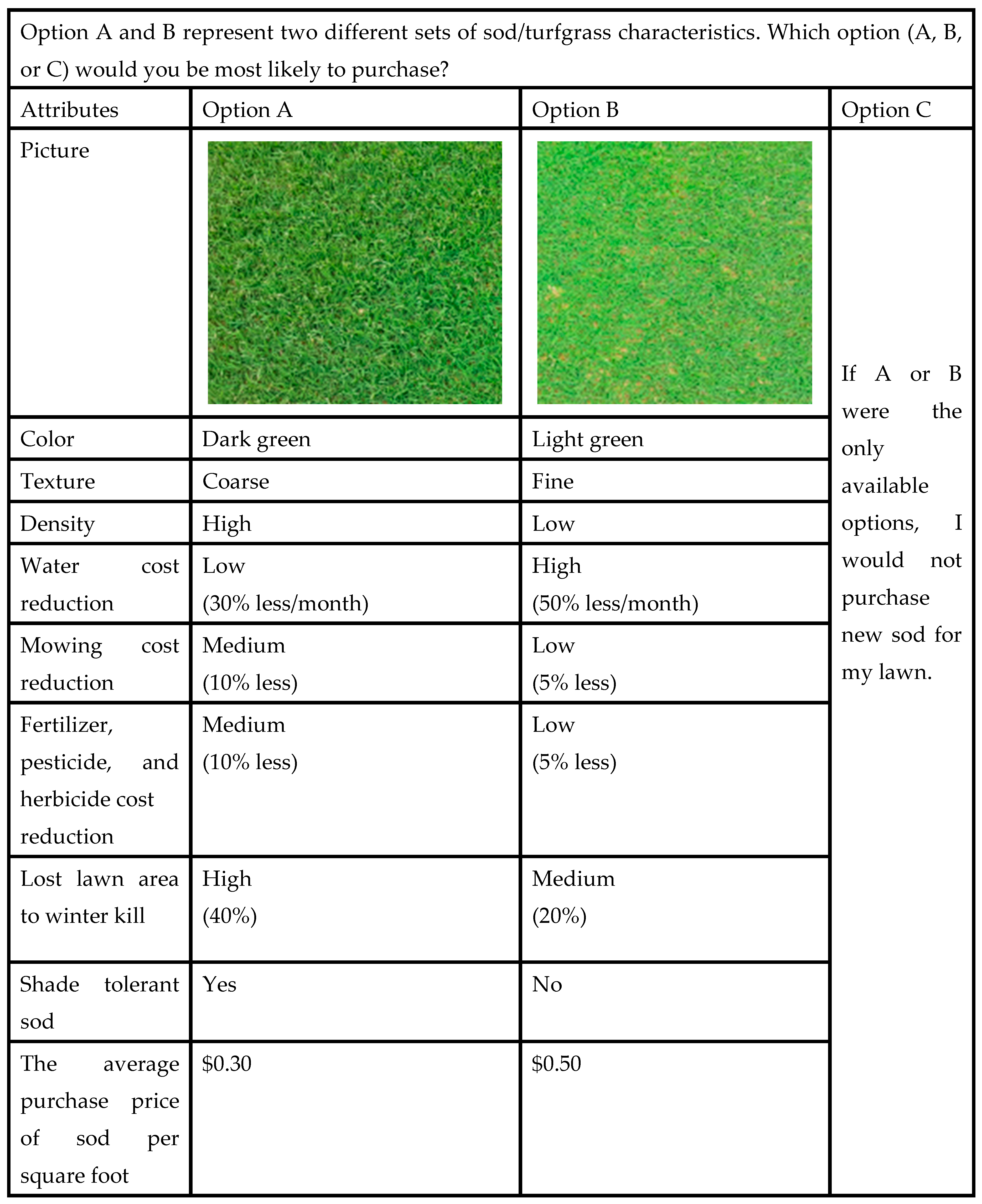

Table 1.
Turfgrass Attributes and Attribute Levels.
| Attributes | Attribute levels |
|---|---|
| Water cost reduction | Low (30% less/month) Medium (40% less/month) High (50% less/month) |
| Mowing cost reduction | Low (5% less) Medium (10% less) High (15% less) |
| Fertilizer, pesticide, and herbicide cost reduction | Low (5% less) Medium (10% less) High (15% less) |
| Lost lawn area to winter kill | Low (0%) Medium (20%) High (40%) |
| Shade tolerance | No Yes |
| Color | Light green Dark green |
| Density | Low High |
| Texture | Fine Coarse |
| The purchase price of sod per square foot | $0.20, $0.30, $0.40, $0.50 |
Table 2.
Descriptive Statistics of Individuals’ Demographic Characteristics.
| Variables | Mean/Proportion | Standard deviation |
|---|---|---|
| Age | 50.56 | 17.90 |
| Gender | ||
| Male | 0.49 | - |
| Female | 0.51 | - |
| Education | ||
| Less than high school | 0.01 | - |
| High school graduate | 0.26 | - |
| Undergraduate degree | 0.43 | - |
| Graduate degree | 0.31 | - |
| Income | ||
| <$25,000 | 0.12 | - |
| $25,000-$49,999 | 0.21 | - |
| $50,000-$74,999 | 0.21 | - |
| $75,000-$99,999 | 0.14 | - |
| $100,000-$124,999 | 0.08 | - |
| $125,000-$149,999 | 0.09 | - |
| $150,000-$174,999 | 0.06 | - |
| $175,000-$199,999 | 0.04 | - |
| >$200,000 | 0.06 | - |
Table 3.
Estimates of Mixed Logit Model with and without Interaction Terms. .
| Without interaction terms | With interaction terms |
|||
| Attributes | Color (light green) | Density (low) | Texture (fine) | |
|
Direct effect | ||||
| ASC | -1.2968*** (0.1457) |
-1.2721*** (0.1726) |
-1.3211*** (0.1045) |
-1.3044*** (0.1140) |
| 40% water cost reduction | 0.0713*** (0.0168) |
0.0517*** (0.0241) |
0.0790*** (0.0229) |
0.0765*** (0.0219) |
| 50% water cost reduction | 0.1228*** (0.0223) |
0.1139*** (0.0314) |
0.1225*** (0.0314) |
0.1322*** (0.0270) |
| 10% mowing cost reduction | 0.0009 (0.0154) |
0.0131 (0.0190) |
0.0037 (0.0316) |
-0.0015 (0.0168) |
| 15% mowing cost reduction | 0.0261* (0.0144) |
0.0366* (0.0165) |
0.0202* (0.0159) |
0.0183 (0.0154) |
| 10% fertilizer, pesticide, and herbicide cost reduction | 0.0016 (0.0181) |
0.0027 (0.0162) |
-0.0030 (0.0221) |
0.0117 (0.0239) |
| 15% fertilizer, pesticide, and herbicide cost reduction | 0.0226 (0.0189) |
0.0264** (0.0191) |
0.0430** (0.0242) |
0.0363** (0.0199) |
| 20% lost lawn area to winter kill | 0.1290*** (0.0212) |
0.1211*** (0.0247) |
0.1251*** (0.0425) |
0.1174*** (0.0241) |
| 0% lost lawn area to winter kill | 0.1843*** (0.0299) |
0.1741*** (0.0323) |
0.1701*** (0.0447) |
0.1696*** (0.0330) |
| Shade tolerance | 0.1129*** (0.0175) |
0.1277*** (0.0216) |
0.1366*** (0.0167) |
0.1264*** (0.0213) |
| Light green | -0.1829*** (0.0293) |
-0.1785*** (0.0252) |
-0.1506*** (0.0192) |
-0.1869*** (0.0403) |
| Low density | -0.1660*** (0.0326) |
-0.1607*** (0.0216) |
-0.1563*** (0.0242) |
-0.1716*** (0.0238) |
| Fine texture | -0.0080 (0.0167) |
-0.0053 (0.0190) |
-0.0065 (0.0337) |
0.0067 (0.0187) |
| Indirect effect (from interaction terms with aesthetic attributes) | ||||
| 40% water cost reduction | - | 0.0014 (0.0301) |
0.0228 (0.0261) |
-0.0150 (0.0301) |
| 50% water cost reduction | - | -0.0214 (0.0314) |
0.0414 (0.0305) |
0.0190 (0.0281) |
| 10% mowing cost reduction | - | 0.0016 (0.0325) |
-0.0069 (0.0644) |
-0.0244 (0.0258) |
| 15% mowing cost reduction | - | 0.0441 (0.0355) |
0.0217 (0.0285) |
0.0165 (0.0266) |
| 10% fertilizer, pesticide, and herbicide cost reduction | - | -0.0261 (0.0320) |
-0.0086 (0.0364) |
-0.0024 (0.0299) |
| 15% fertilizer, pesticide, and herbicide cost reduction | - | -0.0209 (0.0347) |
-0.0010 (0.0212) |
0.0050 (0.0250) |
| 20% lost lawn area to winter kill | - | 0.0043 (0.0283) |
-0.0236 (0.0277) |
-0.0005 (0.0281) |
| 0% lost lawn area to winter kill | - | -0.0238 (0.0280) |
-0.0261 (0.0335) |
-0.0181 (0.0281) |
| Shade tolerance | - | -0.0457 (0.0436) |
-0.0890*** (0.0275) |
0.0201 (0.0297) |
| Number of observations | 10,980 | 10,980 | 10,980 | 10,980 |
Standard errors are in parentheses. ***, **, and * indicate p<0.01, p<0.05, and p<0.10, respectively.
Table 4.
WTPs with Interaction Terms.
| Attributes | Color (light green) | Density (low) | Texture (fine) |
|---|---|---|---|
| 40% water cost reduction | 0.0531 (0.0401) |
0.1018*** (0.0353) |
0.0614* (0.0364) |
| 50% water cost reduction | 0.0924** (0.0444) |
0.1639*** (0.0408) |
0.1512*** (0.0394) |
| 10% mowing cost reduction | 0.0146 (0.0390) |
-0.0032 (0.0637) |
-0.0259 (0.0309) |
| 15% mowing cost reduction | 0.0807** (0.0397) |
0.0418 (0.0319) |
0.0348 (0.0308) |
| 10% fertilizer, pesticide, and herbicide cost reduction | -0.0234 (0.0364) |
-0.0115 (0.0506) |
0.0093 (0.0377) |
| 15% fertilizer, pesticide, and herbicide cost reduction | 0.0055 (0.0409) |
0.0421 (0.0379) |
0.0413** (0.0315) |
| 20% lost lawn area to winter kill | 0.1253*** (0.0360) |
0.1015** (0.0504) |
0.1168*** (0.0373) |
| 0% lost lawn area to winter kill | 0.1503*** (0.0405) |
0.1440*** (0.0511) |
0.1515*** (0.0438) |
| Shade tolerance | 0.0819* (0.0479) |
0.0477 (0.0314) |
0.1466*** (0.0362) |
Standard errors are in parentheses. ***, **, and * indicate p<0.01, p<0.05, and p<0.10, respectively.
Table 5.
Rankings of Consumers’ WTP over Turfgrass Attributes.
| Without interaction terms | With interaction terms |
|||||||
|---|---|---|---|---|---|---|---|---|
| Color (light green) | Density (low) | Texture (fine) | ||||||
| Attributes | Relative importance (%) | Ranking | Relative importance (%) | Ranking | Relative importance (%) | Ranking | Relative importance (%) | Ranking |
| Water cost reduction | 19.37 | 3 | 19.75 | 2 | 46.98 | 1 | 33.79 | 2 |
| Mowing cost reduction | 5.43 | 4 | 17.24 | 4 | 0.00 | 4 | 0.00 | 4 |
| Fertilizer, pesticide, and herbicide cost reduction | 0.00 | 5 | 0.00 | 5 | 0.00 | 4 | 0.00 | 4 |
| Lost lawn area to winter kill | 51.72 | 1 | 45.50 | 1 | 42.58 | 2 | 38.99 | 1 |
| Shade tolerance | 23.47 | 2 | 17.51 | 3 | 10.43 | 3 | 27.22 | 3 |
Table 6.
Change in WTP for 50% Water Cost Reduction under Water Policy Scenarios.
| Policy scenario | Attribute | WTPbefore | WTPafter | T-test for comparing WTPs |
|---|---|---|---|---|
| 25% water rate increase | 50% water cost reduction | 0.0912*** (0.0335) |
0.9267*** (0.1384) |
0.8356*** (0.1424) |
| 50% water rate increase | 50% water cost reduction | 0.0720* (0.0431) |
0.3326*** (0.1179) |
0.2606** (0.1255) |
| 100% water rate increase | 50% water cost reduction | 0.1800*** (0.0468) |
0.2128*** (0.0488) |
0.0328 (0.0676) |
| Restriction for the watering lawn: Even or odd days a week | 50% water cost reduction | 0.0811** (0.0323) |
0.0932*** (0.0305) |
0.0121 (0.0445) |
| Restriction for the watering lawn: Two days a week | 50% water cost reduction | 0.2495 (0.7274) |
0.2629*** (0.0400) |
0.0134 (0.7285) |
| Restriction for the watering lawn: One day a week | 50% water cost reduction | 0.2663*** (0.0614) |
0.4117** (0.1978) |
0.1454 (0.2071) |
Standard errors are in parentheses. ***, **, and * indicate p<0.01, p<0.05, and p<0.10, respectively.
| [1] | Many studies find that, among non-price policies, mandatory water restriction policies are more effective than voluntary water conservation policies [10,12]. Kenney et al. (2004) [10] show that once a week watering restriction decreases water consumption more than twice a week restriction. On the other hand, Ozan and Alsharif (2013) [11] find that water consumption decreases with the number of watering restriction, i.e., twice a week watering restriction is more effective than once a week restriction.
|
| [2] | Yue et al. (2012) [8] note that homeowners would prefer drought-tolerant plants under the water price increasing policy. However, the study does not estimate the effect of water-conservation policy on consumer preference for turfgrass attributes. |
| [3] | Subscripts, i, j, and t, are henceforth suppressed for the sake of notational simplicity. |
| [4] | In many studies using effect coding, the WTP from effect coding multiplied by 2 is typically considered the same as the WTP from the dummy coding due to the difference in base coding. However, Hu et al. (2022) [20] demonstrate that this interpretation is appropriate only when the attribute level is two. When the level of attribute is more than two, more general method such as equation (7) needs to be used for the interpretation of estimated WTPs from effect coding. |
| [5] | The survey (IRB-21-93) was approved by the Institutional Review Board (IRB) at Oklahoma State University. |
| [6] | Fessler et al. (2022) [22] removed respondents who spent less than 4 minutes to complete the whole survey (including four choice tasks and demographic questions) and who showed questionable responses during choice experiments. Previous studies also used trap questions [23], eye-tracking [24], and attribute non-attendance (ANA) analysis [25] to address participants’ inattention problem. |
| [7] | Irrigation restriction policies typically include a combination of total irrigation hours a week, time of irrigation, and voluntary or mandatory participation. Since it is difficult to consider all these combinations in our experimental design, this study focuses on the frequency of outdoor watering. |
| [8] | We tried both the Halton draw method and the pseudo-Monte Carlo draw method and found that both methods yielded almost the same results. We here present results from the Halton draw method. |
| [9] | We also estimated the same water policy effects on the attribute of 40% water cost reduction and found similar results (the policy of 25% water rate increase effectively raised the WTP at the 1% level), but overall the policy effects were lower than the results from the attribute of 50% water cost reduction. |
Disclaimer/Publisher’s Note: The statements, opinions and data contained in all publications are solely those of the individual author(s) and contributor(s) and not of MDPI and/or the editor(s). MDPI and/or the editor(s) disclaim responsibility for any injury to people or property resulting from any ideas, methods, instructions or products referred to in the content. |
© 2023 by the authors. Licensee MDPI, Basel, Switzerland. This article is an open access article distributed under the terms and conditions of the Creative Commons Attribution (CC BY) license (http://creativecommons.org/licenses/by/4.0/).
Copyright: This open access article is published under a Creative Commons CC BY 4.0 license, which permit the free download, distribution, and reuse, provided that the author and preprint are cited in any reuse.


